Scaling of inefficiencies in the U.S. equity markets: Evidence from three market indices and more than 2900 securities
Abstract
Using the most comprehensive, commercially-available dataset of trading activity in U.S. equity markets, we catalog and analyze quote dislocations between the SIP National Best Bid and Offer (NBBO) and a synthetic BBO constructed from direct feeds. We observe a total of over 3.1 billion dislocation segments in the Russell 3000 during trading in 2016, roughly 525 per second of trading. However, these dislocations do not occur uniformly throughout the trading day. We identify a characteristic structure that features more dislocations near the open and close. Additionally, around 23% of observed trades executed during dislocations. These trades may have been impacted by stale information, leading to estimated opportunity costs on the order of $2 billion USD. A subset of the constituents of the S&P 500 index experience the greatest amount of opportunity cost and appear to drive inefficiencies in other stocks. These results quantify impacts of the physical structure of the U.S. National Market System.
keywords:
Assymetric Information, Empirical Finance, Equities, Financial Markets, Imperfections, Market Microstructure, ScalingD50, D82, G14
1 Introduction
Securities markets utilize auction mechanisms to facilitate the valuation and trade of assets (de la Vega, 1688; Bachelier, 1900; Knight, 1921; Fama, 1965). Implementation details of these markets, including the auction mechanism, computing and communication infrastructure, as well as information dissemination policies, impact their informational and economic efficiency (Akerlof, 1970; Easley and O’hara, 1987). These market microstructure factors have been increasingly considered in recent analyses of market efficiency (Wissner-Gross and Freer, 2010; Ding et al., 2014; Mackintosh, 2014; Adrian, 2016), and we contribute to this body of work.
1.1 Modern U.S. market
We investigate a broad subset of the equities traded in the U.S. National Market System (NMS), a network of stock exchanges located in the U.S., since it is the proverbial center of the world equity markets. In particular, we focus on constituents of the Russell 3000 Index, which is compiled by FTSE International Ltd. and contains roughly 3000 of the largest equities traded on the NMS. The selected sample represents the vast majority of the equities traded in the U.S. and can serve as a nearly comprehensive cross-section of publicly traded equities from which the observation and assessment of microstructure quantities can be made.
Summary statistics of the realized opportunity cost (ROC) aggregated across all studied securities and all of calendar year 2016. The total ROC of this sample is over $2B USD. We discuss statistical characteristics of ROC extensively in Section 6. Row 10 shows that the average differing trade moves approximately 6.51% more value than the average trade. This indicates a qualitative shift in trading behavior during dislocations. 1 Realized Opportunity Cost $2,051,916,739.66 2 SIP Opportunity Cost $1,914,018,654.41 3 Direct Opportunity Cost $137,898,085.25 4 Trades 4,745,033,119 5 Diff. Trades 1,124,814,017 6 Traded Value $28,031,002,997,692.75 7 Diff. Traded Value $7,077,357,462,641.67 8 Percent Diff. Trades 23.71 9 Percent Diff. Traded Value 25.25 10 Ratio of 9 / 8 1.0651
Using the most comprehensive dataset of NMS messages commercially available, we enumerate and describe dislocation segments (DS) and realized opportunity costs (ROC), defined in Section 5, in Russell 3000 securities and a selection of exchange-traded funds (ETFs) during calendar year 2016. Extending Tivnan et al. (2020), we observe over DSs in the National Market System during the period of study. Consistent with Tivnan et al. (2020), we define a dislocation as the market state when the National Best Bid and Offer (NBBO) and a synthetic, Direct Best Bid and Offer (DBBO) simultaneously display different prices. Any trade that executes during a dislocation is called a differing trade. Row 8 of Table 1.1 shows that 23.71% of all trades were differing trades. Differing trades may have been influenced by stale quote information, so we used them to calculate ROC. However, some trades may have been executed in this period intentionally, so we only include differing trades that executed at either of the two NBBO quotes. This results in a conservative estimate of total ROC, $2,051,916,739.66 across the Russell 3000 in 2016, as depicted in Row 1 of Table 1.1. Table 1.1 depicts the total number of dislocations that we observed in 2016, delineating those that persisted for a minimum duration and those greater than the minimum magnitude (i.e., tick size). Despite recent technological upgrades to market infrastructure, the chief economist at Nasdaq confirms that latencies of 500 microseconds remain material in 2020 for the execution of latency arbitrage strategies Mackintosh (2020).
Total number of dislocation segments in mutually-exclusive market categories. Number of opportunities is calculated unconditioned, conditioned on duration, and conditioned on both duration and magnitude. Category Duration Magnitude Count Dow - - 120,355,462 - 65,073,196 1¢ 2,872,734 SPexDow - - 1,126,186,592 - 530,499,458 1¢ 51,187,430 RexSP - - 1,888,686,248 - 704,416,718 1¢ 110,447,787
1.2 Scaling in finance
Mandelbrot (1997, 2013) was one of the first to characterize the scaling properties of price returns in modern markets. The scaling of returns was later revisited by Stanley and Plerou (2001), Cont (2001), as well as Patzelt and Bouchaud (2018). Beyond returns in price time series, additional financial variables have been found to display scaling properties. Market indices and foreign exchange rates (Di Matteo, 2007) as well as share volume and number of trades (Stanley et al., 2008) adhere to scaling properties.
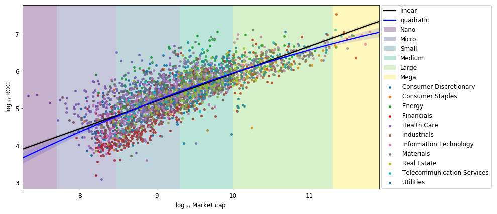
Leveraging the large number of securities under study and the broad range of market capitalization (MC) covered, we examine scaling relationships between DSs, ROC, and MC. DSs occur in equities of all sizes. While DS are more frequent in equities with larger MC, the distributions of their qualities, such as their magnitude and duration, are more extreme among equities with smaller MC. We find a strong positive correlation between MC and ROC, show in Figure 1. A similar relationship is seen between MC-total trades and MC-differing trades in Figure 6. The majority of ROC is generated by equities in the S&P 500 that are not also in the Dow (termed the SPexDow). The SPexDow also Granger-causes ROC in other mutually-exclusive market categories (Dow 30 and Russell 3000 less the S&P 500, or RexSP), pointing to its centrality in the U.S. equities market.
In the following sections, we first provide a brief overview of the U.S. National Market System. We then detail our data, the available and used fields, and summarize the equities studied. After describing statistics of DSs, including distributions of start times and durations, we move to analysis of ROC, providing summary statistics, comparisons across mutually-exclusive market categories, and correlation along with Granger-causality analyses. We close with a brief exploration of exchange-traded funds (ETFs), a discussion of results, and possibilities for future work.
1.3 Empirical Studies of Modern U.S. Markets
In a recent report to its government oversight committee, the U.S. Securities and Exchange Commission (SEC) offered the following characterization of the prevailing literature which relates to our study: “It is unsurprising that academic studies generally are narrowly focused, as the amount of data, computing power and sophistication necessary to engage in broader study are daunting and costly, and relevant data may not be widely available or easily accessible.” (U.S. Securities and Exchange Commission, 2020b, p. 45). Given these constraints, we are aware of only two other recent studies which also used comprehensive, market data to analyze the modern U.S. market.
In the first study, Wah (2016) calculated the potential opportunities for latency arbitrage on the S&P 500 in 2014 using data from the SEC’s MIDAS platform (U.S. Securities and Exchange Commission, 2013a). Using similar data to that for our study, Wah identified price discrepancies that could serve as latency arbitrage opportunities. She then examined the potential profit to be made by an infinitely fast arbitrageur taking advantage of these opportunities. Wah estimates that this idealized arbitrageur could have captured $3.0B USD from latency arbitrage in 2014, which is similar to our conservative calculations of approximately $2.1B USD in ROC from actual trades in 2016.
The second study was Aquilina et al. (2020), which used message data from 2015 to quantify aspects of latency arbitrage in global equity markets. The authors note the frequent yet fleeting occurrence of latency arbitrage opportunities and estimate profits from latency arbitrage in 2018 at $4.8B USD globally, including $2.8B USD in the U.S. equity market.
Both the Wah and Aquilina et al. studies relied on affiliations with regulatory agencies and their respective data. This reliance on regulatory data supports the SEC observation that “relevant data may not be widely available or easily accessible.”
2 Market Overview
The U.S. equities market, known as the National Market System (NMS), is composed of 13 National Securities Exchanges. Each exchange contributes to price discovery through the interactions of market participants, mediated by an auction mechanism. Another core component of the NMS is a collection of approximately 40 alternative trading systems (ATSs) (Tuttle, 2013), also known as dark pools. ATSs provide limited pre-trade transparency, which can allow market participants to reduce the market impact of their trades, but have limited participation in price discovery as a result. Each exchange and ATS accumulates orders whose execution conditions have not been met in an order book. Resting orders are matched with incoming marketable orders based on a priority mechanism, commonly price-time priority (Bessembinder, 2001). Traders often have access to a variety of order types that allow them to tailor how they interact with the market (Nasdaq, 2017; New York Stock Exchange, 2020; Chicago Board Options Exchange, 2020; Exchange, 2020). The top of the book at each exchange, the resting bid with the highest price and the resting offer with the lowest price, is called the best bid and offer (BBO). BBOs from across the NMS are aggregated by one of the Securities Information Processors (SIP) to form the national best bid and offer (NBBO) (The Consolidated Tape Association, 2020; The UTP Plan, 2020). Under Regulation National Market System (Reg. NMS), trades must execute at a price that is no worse than the NBBO, though exceptions exist (e.g. intermarket sweep orders) (U.S. Securities and Exchange Commission, 2005).
Market participants in the NMS have several options of data products to fuel their trading decisions. In addition to the dissemination of the NBBO, each SIP provides data feeds containing all quotes and trades that occur in their managed securities. Information feeds offered by each exchange, referred to as direct feeds, can provide similar information with lower latency than the SIP data feeds. Direct feeds can also provide additional data, such as the resting volume at all price points, commonly called depth-of-book information. Information asymmetries between data products lead to DSs, which can impact trading decisions and outcomes.
The NMS is regulated by the U.S. Securities and Exchange Commission (SEC), a federal agency, and self-regulated by the Financial Industry Regulatory Authority (FINRA), a professional organization. FINRA polices its members and ensures they adhere to SEC rules and other professional guidelines, while SEC designs, implements, and enforces rules that are intended to promote market stability and economic efficiency. The physical structure of the NMS, in conjunction with the existence and usage of multiple distinct information feeds, leads to the creation of DSs and associated ROC. On Dow 30 equities, over 120 million DSs and over $160M USD in ROC were cataloged during calendar year 2016 (Tivnan et al., 2020).
Our calculations provide a conservative estimate of ROC from actual trades in the U.S. equity markets in 2016. Therefore, we identify some relevant literature on trade execution (U.S. Securities and Exchange Commission, 2013b); namely, where and when trades occur. First, trading is not instantaneous. Delays, or latencies, exist throughout the NMS. Second, not all trading activity occurs at a national exchange or an ATS. Instead of routing an order to one of these market venues, a broker may execute the order against the broker’s own inventory of that stock. This process of retaining customers’ orders internal to the brokerage is called “internalization” (U.S. Securities and Exchange Commission, 2000). In addition to matching customers’ orders against the broker’s inventory of a particular stock, internalization also includes instances when a broker may route customers’ orders to a market-maker under a Payment for Order Flow (PFOF) agreement. Even without charging commissions for trades, brokers may generate revenue from executing trades via PFOF (U.S. Securities and Exchange Commission, 2007). To mitigate potential conflicts of interest, each broker is required to ensure that its customers’ orders execute against best prices, as determined by the NBBO.
Trade execution problems may still arise from PFOF. In a public statement announcing its fine against a prominent market-maker, the SEC noted the use of algorithms which were used to avoid paying best prices on internalized orders. Per the SEC, “these algorithms were triggered when they identified differences in the best prices on market feeds, comparing the SIP feeds to the direct feeds from exchanges” (U.S. Securities and Exchange Commission, 2017). The reader will note that this market state, what the SEC has identified as “differences in best prices on market feeds,” is the very same state that we have defined here as a market dislocation.
PFOF remains a controversial practice. More recently, another market-maker settled allegations that it did not ensure best prices for the internalization of its customers’ orders (Michaels, 2019).
We found references to internalization and PFOF dating back to 1994, when annual revenues from PFOF exceeded $500M USD across all U.S. brokers (Power, 1994). Some studies identified the potential for conflicts of interest from PFOF, but claimed that these conflicts could be mitigated by the adoption of minimum tick sizes of a penny (i.e., decimalization) (Chordia and Subrahmanyam, 1995; Easley et al., 1996). Though the SEC adopted decimalization in 2000 (U.S. Securities and Exchange Commission, 2020a), PFOF remains a lucrative practice. In the first half of 2020, four brokers in the U.S. generated more than $1B USD in revenue from PFOF (Wursthorn and Choi, 2020).
This brief overview of the U.S. equities market only provides context for the following sections and is far from complete. We refer the reader to Tivnan et al. (2020) for a more complete discussion.
3 Indices
Many of our results are centered around the components of three of the most popular equity indices: Dow Jones Industrial Average, S&P 500, and the Russell 3000. Indices measure the performance of a bucket of securities. The choice of the underlying securities is often to be representative of a market segment. Indices may not be directly purchased in the same way as an equity, but may be tracked by Exchange Traded Funds (ETFs) and mutual funds.
The Dow Jones Industrial Average, from here on referred to as the Dow, is a price weighted index that aims to provide an overview of the U.S. economy (S&P Dow Jones Indices, 2020a). The Dow consists of thirty S&P 500 constituents, covering all industries except for utilities and transportation.
The S&P 500 is a market capitalization weighted index of 500 large US based companies referred to by it’s creators as “the gauge of the market economy”. The index is considered by many to be representative of the US stock market as a whole and is a primary holding among passive investors. To be included in the index, as of 2016, a company must meet the following criteria (S&P Dow Jones Indices, 2020b).
-
•
Be a U.S. Company
-
•
Have a market capitalization greater than $5.3 billion
-
•
Be highly liquid
-
•
Have a public float of at least 50% of outstanding shares
-
•
Had positive earnings in the most recent quarter
-
•
The sum of the last four consecutive quarterly earnings must be positive
-
•
Be listed on a major exchange
Meeting these criteria does not guarantee inclusion, and failing to uphold these standards does not necessarily result in immediate expulsion from the index. S&P 500 constituents are chosen by S&P Global, and the index is updated regularly, though not on any fixed schedule.
The Russell indexes are passively constructed (no human in the loop) based on a transparent set of rules including (FTSE Russell, 2020b):
-
•
Be a U.S. Company
-
•
Be listed on a major exchange
-
•
Have a share price $1
-
•
Have a market capitalization $30M
-
•
Have a public float 5%
The Russell 3000 consists of the largest 3000 firms by market capitalization meeting the above criteria, or the entire eligible set, whichever is smaller. The index undergoes an annual reconstruction in June and is augmented quarterly with the addition of Initial Public Offerings (IPO). This methodology results in the Russell 3000 being a strict superset of the S&P 500.
For our analysis we focus on constituents of these indices, rather the index itself. Thus, differing weighting methodologies used by these indices have no effect on our analysis. We also note that some companies have multiple common stocks, one for each share class, and that each index handles the inclusion of multiple share classes differently.
4 Data
We use a dataset comprised of every quote and trade message that was disseminated on one of the SIP or direct feeds during the period of study. This dataset features comprehensive coverage of the stocks under study, is collected from a single location (Carteret, NJ), and is time stamped upon arrival, thus limiting clock synchronization issues. Thesys Technologies collected and curated this data (Thesys Technologies, 2020), and also provided data for the SEC’s MIDAS (U.S. Securities and Exchange Commission, 2013a) at the time of collection. Index membership, Global Industry Classification Standard (GICS) sector classification, and MC data were obtained from a Bloomberg Terminal.
The indices we consider are subject to frequent changes in membership. To simplify our analysis we consider the Dow 30 and S&P 500 as they stood on Jan. 1, 2016. For the Russell 3000 we consider the constituents as listed in the June 2016 construction, excluding those that were not publicly traded on Jan. 1, 2016. Constituents of the indices under study were curated to only include companies that survived as a publicly traded entity on a national exchange for the entire calendar year of 2016. Companies that were delisted for any reason (e.g. bankruptcy or buyout) were excluded, in addition to those who were acquired by an out-of-study firm. Mergers between in-sample companies did not result in exclusion. Curating the stocks under study in this way allows us to avoid issues caused by IPOs and delistings.
Many companies in our dataset changed their ticker symbol over the course of the calendar year and thus appear as a different entity in the data. To study a company over a long time period it is necessary to know all tickers it traded under and when the ticker changes occurred. There is no consolidated public record of these ticker changes, so we tracked them via an extensive review of press releases. These ticker changes were then validated by observing changes in trading activity in the old and new ticker on the date of the change using the Thesys data archive.
This curation reduced the Russell 3000 from 3005 stocks to 2903, the S&P 500 from 500 stocks to 472, and did not impact the 30 members of the Dow. We denote the curated version of an existing index by appending a prime to the respective base index (e.g. Dow 30 Dow 30′). We then construct two additional stock groups, RexSP and SPexDow, by taking the appropriate set difference, e.g. SPexDow = S&P 500′ - Dow 30′. Finally, all companies in our dataset were classified by their MC as it stood in the beginning of Q4 2016 using the classes defined in Table 4. Our dataset covers approximately 98% of all publicly traded U.S. equities by MC (FTSE Russell, 2020a). Tables 4 - 4 provide summary statistics and distribution of these equities across GICS sector, MC, and market category, for several indices.
Composition of indexes under study by market capitalization (MC) classification as of Q4 2016. The composition of various indexes is displayed by the percentage of index constituents that are a member of each given index (% by #) and by the weighting of those constituents (% by MC). Class Statistic Russ 3K′ RexSP S&P 500′ SPexDow Dow 30′ Nano % by # 0.14 0.16 0.00 0.00 0.00 % by MC 0.00 0.00 0.00 0.00 0.00 Count 4 4 0 0 0 Micro % by # 11.51 13.74 0.00 0.00 0.00 % by MC 0.26 1.09 0.00 0.00 0.00 Count 334 334 0 0 0 Small % by # 42.89 51.13 0.42 0.45 0.00 % by MC 4.37 18.50 0.01 0.02 0.00 Count 1,245 1,243 2 2 0 Mid % by # 30.35 32.21 20.76 22.17 0.00 % by MC 15.11 53.19 3.37 4.72 0.00 Count 881 783 98 98 0 Large % by # 14.50 2.71 75.21 75.79 66.67 % by MC 56.68 20.72 67.77 77.59 43.28 Count 421 66 355 335 20 Mega % by # 0.62 0.04 3.60 1.58 33.33 % by MC 23.58 6.50 28.85 17.67 56.72 Count 18 1 17 7 10
Market Capitalization (MC) statistics of equities under study broken out by Global Industry Classification Standard (GICS) sector as of Q4 2016. The composition of various indexes is displayed by the percentage of index constituents that are a member of each given sector (% by #) and by the weighting of those constituents (% by MC). Additionally, the MC of the smallest and largest constituent for each index in each category is displayed. Sector Statistic Russ 3K′ RexSP S&P 500′ SPexDow Dow 30′ Consumer Discretionary % by # 14.92 14.52 16.95 17.19 13.33 % by MC 12.97 16.40 11.92 13.10 8.98 Count 433 353 80 76 4 ($) MC Min 95,330,024 95,330,024 1,244,719,232 1,244,719,232 84,654,022,656 ($) MC Max 356,313,137,152 89,539,158,016 356,313,137,152 356,313,137,152 165,862,064,128 Consumer Staples % by # 4.03 3.41 7.20 7.01 10 % by MC 8.54 3.83 9.99 9.69 10.74 Count 117 83 34 31 3 ($) MC Min 114,570,432 114,570,432 9,794,159,616 9,794,159,616 178,815,287,296 ($) MC Max 224,997,457,920 17,508,790,272 224,997,457,920 150,058,582,016 224,997,457,920 Energy % by # 5.20 4.73 7.63 7.69 6.67 % by MC 6.57 4.71 7.14 5.83 10.40 Count 151 115 36 34 2 ($) MC Min 160,502,160 160,502,160 2,427,903,232 2,427,903,232 222,190,436,352 ($) MC Max 374,280,552,448 27,468,929,024 374,280,552,448 116,800,331,776 374,280,552,448 Financials % by # 17.81 18.84 12.50 12.44 13.33 % by MC 15.17 21.99 13.07 14.73 8.91 Count 517 458 59 55 4 ($) MC Min 89,903,488 89,903,488 3,021,111,552 3,021,111,552 34,774,474,752 ($) MC Max 401,644,421,120 401,644,421,120 308,768,440,320 276,779,139,072 308,768,440,320 Health Care % by # 15.23 15.84 12.08 11.99 13.33 % by MC 12.49 9.12 13.53 13.19 14.38 Count 442 385 57 53 4 ($) MC Min 21,050,850 21,050,850 1,478,593,408 1,478,593,408 152,328,667,136 ($) MC Max 313,432,473,600 18,889,377,792 313,432,473,600 108,768,911,360 313,432,473,600 Industrials % by # 13.47 13.41 13.77 13.57 16.67 % by MC 10.40 11.03 10.20 9.91 10.94 Count 391 326 65 60 5 ($) MC Min 58,695,636 58,695,636 2,821,674,240 2,821,674,240 54,259,630,080 ($) MC Max 279,545,937,920 13,281,452,032 279,545,937,920 100,041,220,096 279,545,937,920 Information Technology % by # 14.40 14.60 13.35 12.90 20 % by MC 21.40 13.81 23.74 20.93 30.74 Count 418 355 63 57 6 ($) MC Min 114,370,240 114,370,240 3,334,570,240 3,334,570,240 151,697,113,088 ($) MC Max 617,588,457,472 32,402,583,552 617,588,457,472 538,572,161,024 617,588,457,472 Materials % by # 4.55 4.40 5.30 5.43 3.33 % by MC 3.26 5.83 2.47 3.02 1.11 Count 132 107 25 24 1 ($) MC Min 103,733,456 103,733,456 2,823,849,728 2,823,849,728 63,809,703,936 ($) MC Max 69,704,540,160 69,704,540,160 63,809,703,936 46,132,944,896 63,809,703,936 Real Estate % by # 6.61 6.99 4.66 4.98 0.00 % by MC 3.89 8.67 2.41 3.38 0.00 Count 192 170 22 22 0 ($) MC Min 161,591,616 161,591,616 7,130,559,488 7,130,559,488 0.00 ($) MC Max 55,830,577,152 24,264,243,200 55,830,577,152 55,830,577,152 0.00 Telecommunication Services % by # 1.03 1.03 1.06 0.90 3.33 % by MC 2.40 1.82 2.57 2.09 3.79 Count 30 25 5 4 1 ($) MC Min 285,299,072 285,299,072 3,964,831,488 3,964,831,488 217,610,731,520 ($) MC Max 261,176,721,408 47,389,126,656 261,176,721,408 261,176,721,408 217,610,731,520 Utilities % by # 2.76 2.22 5.51 5.88 0.00 % by MC 2.91 2.78 2.95 4.13 0.00 Count 80 54 26 26 0 ($) MC Min 141,720,064 141,720,064 3,867,331,328 3,867,331,328 0.00 ($) MC Max 57,253,351,424 12,880,323,584 57,253,351,424 57,253,351,424 0.00
Makeup of market indexes by number of constituents as of Q4 2016. Additionally, the Market Capitalization (MC) of the smallest and largest constituent for each index is displayed along with the sum of all constituent MCs. Russ 3K′ RexSP S&P 500′ SPexDow Dow 30′ Count 2,903 2,431 472 442 30 ($) MC Sum 26,217,754,755,404 6,177,292,648,268 20,040,462,107,136 14,303,673,004,544 5,736,789,102,592 ($) MC Min 21,050,850 21,050,850 1,244,719,232 1,244,719,232 34,774,474,752 ($) MC Max 617,588,457,472 401,644,421,120 617,588,457,472 538,572,161,024 617,588,457,472
5 Methods
Our work investigates the occurrence of DSs and ROC arising from quote discrepancies between the SIP and direct feeds. Similar concepts have been discussed in empirical market microstructure literature (Arnuk and Saluzzi, 2009; Jarrow and Protter, 2012; Hasbrouck and Saar, 2013; Ding et al., 2014; O’Hara, 2015), though formal definitions vary. We follow the definitions described in Tivnan et al. (2020), which are briefly reviewed below.
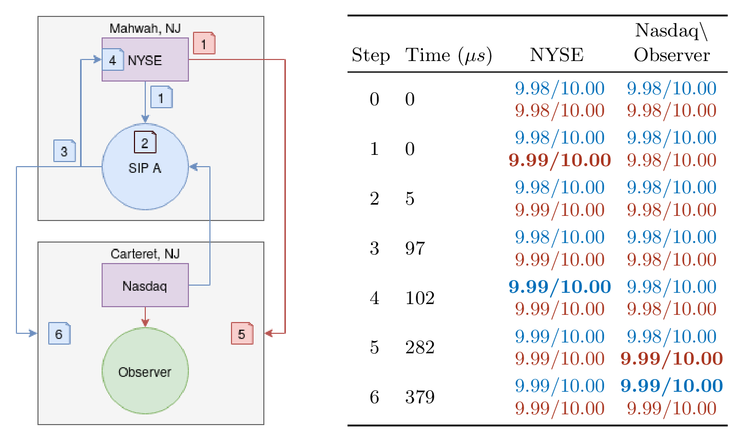
Suppose that there exist two market data feeds, and , each displaying quotes for a single asset. Quotes have the form , where , is the bid price at time , is the offer priceat time , and are the number of shares associated with the bid and offer at time respectively. We observe these feeds from a single, fixed location in Carteret, NJ. A dislocation between these sources of data occurs when the prices of the quotes differ, e.g. or . A DS occurs when the quotes differ and the relationship between the quoted prices remains constant, e.g. or . Figure 2 walks through an example DS occurring on a subset of the NMS using estimates of message transit and processing time for each leg of the journey. In our example a DS starts when a message regarding a quote change in Mahwah reaches our observer in Carteret via a direct feed and ends when the same message arrives via the SIP later. In this single example we see three factors that either alone, or in combination, may cause DSs; differences in processing time, transfer speed, and route (SIP messages require an additional leg). In this example the dislocation was triggered by a single top of book change at NYSE. However, dislocations can occur due to sequences of events occurring across multiple exchanges and SIP processors. Recall that by definition a DS requires two feeds. TAQ data contains only the quotes resulting in a NBBO change as well as all trades. In contrast our dataset contains all quotes sent along the direct feeds as well as all SIP updates. Thus, we can observe events such as our example in Figure 2, an impossibility with TAQ data.
The ROC of using instead of is calculated by combining quote and trade information. Assume that trades take the form , where is the execution price, is the number of traded shares, and is the execution time. If a trade executes at one of the currently quoted prices, e.g. , then the ROC is given by . If the trade executes on the opposite side of the book, e.g. , then the ROC is given by . This allows for a consistent interpretation of the values, where a positive value indicates that displayed a better price for the active trader (higher bid or lower offer) than . The total ROC over an interval is obtained by taking the sum of ROC values from all trades that occurred in that interval.
We first compute summary statistics and qualitative descriptions of the distributions of DSs and ROC. Additionally, we leverage the large sample of equities to conduct a cross-sectional study of the effect of company “size” on these microstructure quantities. We quantify the notion of size of a company by both its MC and its rank in relation to other companies. We also investigate index inclusion effects through the use of disjoint sets of equities and compute aggregate statistics across these sets. Since the S&P 500 is a strict superset of the Dow 30 and the Russell 3000 is a strict superset of the S&P 500, the natural division of the superset of all equities under study is split into three distinct classes: the Dow 30, the S&P 500 excluding the Dow 30 (SPexDOW), and the Russell 3000 excluding the S&P 500 (RexSP). We investigate correlations between these disjoint subsets, and characterize the statistical properties of the time series of DSs and ROC across these disjoint categories. We further explore the relationship between these categories by conducting a Granger causality analysis of aggregated ROC time series (Granger, 1969).
The next section gives results on DSs, including summary statistics and regressions of DSs against MC. We then discuss structure in the intra-day distribution of DS start times and DS duration. Following this, we provide statistics of the ROC across the market as a whole and again within mutually-exclusive market categories. We then explore statistical properties of the ROC time series. We close with an overview of the statistics of ETF DSs and ROC, contrasting these with those of the market as a whole.
6 Results
6.1 Dislocation Segments
DSs can occur when quotes displayed by distinct information feeds differ. We cataloged all DSs occurring in the equities under study and present summary statistics along with qualitative comparisons of their distributions and higher-order moment statistics. Table 8 - 8 display means of summary statistics of DSs for each mutually-exclusive market category under study.
We will use the notation to denote an average of the quantity conditioned on the condition . These averages are interpreted as the quantity conditioned on condition averaged over all securities and all times of observation; defining the number of instances of the quantity having condition as , we have
| (1) |
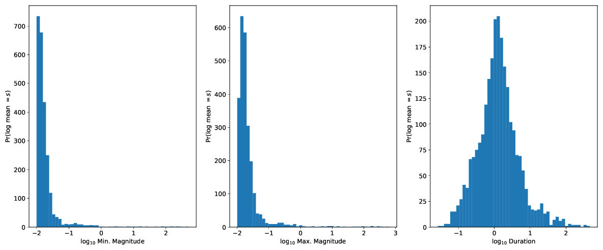
Tables 8 - 8 show that, on average, there were more DSs in Dow 30 securities than in SPexDow or RexSP securities. However, the average maximum magnitude of DSs in the Dow30 is lower than those of the SPexDow, which in turn are lower than those of the RexSP. In particular, actionable DSs (those with duration ) with magnitude $0.01 exhibit more extreme behavior in the SPexDow and RexSP than in the Dow. On average, the median maximum magnitude in the Dow 30 among actionable DSs was , while in the SPexDow we observed and in the RexSP , a roughly one-cent increase in the median maximum magnitude of a DS in each mutually-exclusive market category. Examples of distributions of these quantities are given in Figure 3, where the distributions of the means of minimum magnitude, maximum magnitude, and duration are plotted for the RexSP.
These results provide evidence for the existence of a MC scaling effect in DSs. Securities with larger MC tend to feature higher trading volume and more frequent occurrence of DSs, but these DSs tend to be smaller in magnitude on average. More frequent trading implies a lower probability that prices across differing information feeds will diverge by large magnitudes.
Since DSs are not distributed evenly throughout the day in the Dow 30 (Tivnan et al., 2020), we examine their distribution in the SPexDow and the RexSP as well. Appendix 9 contains figures displaying the distribution of DS start times plotted modulo day and aggregated over the year as well as figures displaying the distribution of DS durations for each mutually exclusive market category. Distributions are plotted both without conditioning, conditioned on duration, as well as conditioned on duration and magnitude.
Distributions of start times display predictable structure. In all market categories, there are large peaks at the very beginning and end of the trading day (circa 9:30 AM and 4:00 PM), along with a noticeable and sudden increase in density around 2:00 PM. The peak in density that occurs at the end of the day is most noticeable when the distribution of start times is not conditioned on DS size. These observations correspond with the results found for the Dow 30 in Tivnan et al. (2020). However, along with these granular observations, there also exists structure on shorter timescales. The distribution exhibits self-similarity on the half-hour timescale, with large peaks every half-hour and decreasing density toward a sudden peak at the next half-hour. There is also structure at the five-minute timescale that is noticeable before the 2:00 PM spike in density but does not appear to be present after the spike. (Future work could statistically test for the presence of this structure and for its persistence across multiple timescales.) The structure on shorter timescales is present in all distributions but, again, is more pronounced in distributions not conditioned on magnitude.
Distributions of DS duration are extremely heavy tailed, so we plot them with a log-transformed horizontal axis. All DS duration distributions exhibit one or more peaks in the range , but there is also a distinct and much lower peak in the distribution near approximately one second in length.
S&P 500 Inclusion Effect: Dislocations
As a visual aid to these results, we have included circle plots, as introduced in Tivnan et al. (2020), to demonstrate the non-uniform distribution of DSs that can occur. Figure 4 shows these circle plots for two common stock pairs ((PBI, INCR), (BRK.B, XOM)) on the edges of our indices. The first pair is the smallest common stock in the S&P 500 by MC that remained in the S&P 500 for the entire calender year and the closest component by MC in the RexSP, PBI and INCR respectively. The second pair is the only mega cap in the RexSP and the closest component by MC in the S&P 500 that remained in the S&P 500 for the entire calender year, BRK.B and XOM respectively. We note that BRK.A is not included in the Russell 3000 (FTSE Russell, 2020b) and that XOM is additionally included in the DOW. These common stock pairs underscore the difference in behavior between constituents of the S&P 500 and those not included in the most worlds most widely tracked equity index.
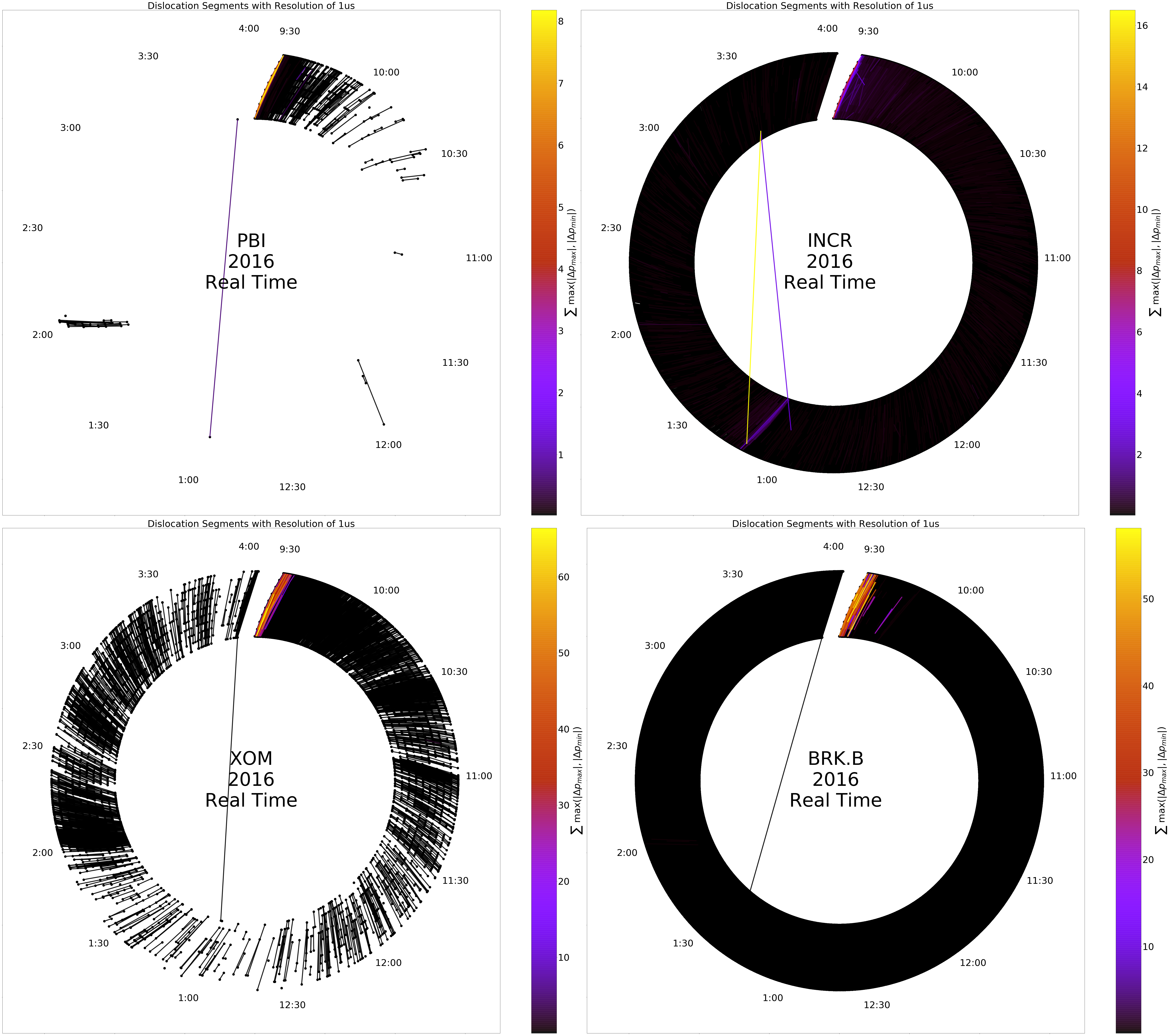
Figure 4 displays the DSs for the above-mentioned common stocks aggregated over a year (modulo day). We see that DSs appear to be more concentrated for S&P 500 constituents with spikes occurring at the beginning of the trading day and at 2:00 pm. Additionally, DSs for S&P 500 constituents tend to have smaller magnitudes, relative to Russell 3000 constituents. We provide circle plots for many more securities on our webpage (Ring IV, 2020).
6.2 Market capitalization
Further evidence for scaling behavior arises from analysis of MC. Tables 4 and 4 display MC statistics broken down by industry sector and categorical size, e.g., micro-cap, mega-cap, etc. MC is significantly positively correlated with ROC. Tables 10 - 10 display results from ordinary least squares regressions predicting ROC using MC and other predictors. A linear fit predicting ROC from MC, total trades, and differing trades gives . A positive coefficient relates ROC to MC, indicating that higher MC is associated with higher ROC. A similar regression is computed including quadratic terms in MC, which has a significant, but weak, negative association with ROC. Similar relationships hold for both the linear and quadratic models when the dependent variable is instead chosen to be total or differing trades.
Though behavior of ROC as a function of MC is generally similar when equities are stratified by sector, some sectors display lower average levels of ROC, differing trades, or total trades when MC is held constant. Equities classified as being in the financial sector generally have a smaller amount of ROC, while equities classified as being in the energy sector exhibit a higher amount of ROC on average. However, there is no clear general trend linking sectors to MC or to ROC.
6.3 Realized opportunity cost
As expected with an increase in the number of analyzed equities from 30 to more than 2900, the amount of ROC rose substantially from the quantity reported in Tivnan et al. (2020), from $160M to $2.05B USD. ROC clearly displays sublinear scaling with the number of studied equities; we do not observe a thousandfold increase in the amount of ROC with a thousandfold increase in the number of equities. The information advantage afforded traders with access to direct feed information is not uniform; though a vast majority of the ROC ($1.91 B) favored the direct feeds in this way, a non-negligible amount of ROC ($137 M) did favor the SIP feeds. Approximately a quarter (23.71%) of all trades observed occurred during a dislocation. The fraction of “differing traded value”—the nominal market value of all differing trades—was slightly higher (25.25%) than the fraction of all trades that were differing trades. The ratio between these two values (25.25% / 23.71% = 1.0651) shows that the average differing trade moves approximately 6.51% more value than the average trade. This indicates a qualitative shift in trading behavior during dislocations.
Securities in the SPexDow account for a median of 2,006,091 differing trades per day, in contrast to the 309,158 in the Dow 30 or 1,921,121 in the RexSP. The median differing traded value per day in the SPexDow was also the highest among the three categories, totaling approximately $14.07T versus the RexSP’s total of $6.7T and the Dow’s total of $3.27T. ROC per share differed across the three categories, with median ROC per share per day of 1.1¢, 1.5¢, 2.1¢for the Dow, SPexDow, and RexSP respectively. ROC per share tends to increase as MC decreases, with lowest ROC per share occurring in the Dow and highest ROC per share occurring in the RexSP. Median total ROC per day on the Dow amounted to $514.8K, while median total ROC per day on the SPexDow totaled $3.384M and on the RexSP amounted to $3.564M. Summary statistics for distributions of ROC for each mutually-exclusive market category are given in Table 8.
Summary statistics for select common stock pairs. BRK.B (paired with XOM) is the only mega cap in the RexSP. PBI (paired with INCR) is the smallest common stock by MC under consideration that remained in the S&P 500 for all of 2016. Note that those in the S&P 500 (green) have a much higher trading volume and ROC then their similarly capitalized counterparts. Ticker MC ($) ROC ($) Trades Diff. Trades Traded Value ($) Diff. Traded Value ($) BRK.B 401,644,421,120 2,278,835.98 5,120,595 1,544,050 70,435,832,686.71 24,162,015,573.13 XOM 374,280,552,448 8,846,416.18 16,146,652 4,479,209 169,057,336,872.77 47,541,675,580.93 PBI 2,821,674,240 726,596.69 2,360,470 488,092 5,766,285,837.56 1,257,265,907.34 INCR 2,820,235,520 487,049.13 904,613 243,855 3,989,174,661.59 1,016,834,174.82
Comparison of the smallest ten common stocks that remained in the S&P 500 for all of 2016 (green) and the ten RexSP common stocks with the closest MC. Rows marked with have significantly (two-sided t-test, p 0.05) higher values for common stocks in the S&P 500. We note that common stocks in the S&P 500 have nearly three times the trading activity and ROC than their similarly capitalized counterparts. Stat. Mean Std. MC ($) ROC ($)† Trades† Diff. Trades† Traded Value ($)† Diff. Traded Value ($)†
It is interesting to consider the distribution of both total ROC and ROC per share by both equity and mutually-exclusive market category. Figure 7 displays ROC of the top 30 and bottom 30 of all securities under study when ranked by ROC. Included in this figure for comparison is the exchange-traded fund SPY, an ETF that tracks the S&P 500. Selected ETFs are also treated separately in Section 6.4. It is notable that the equity with the largest ROC, Bank of America (BAC), has more than twice the ROC of the equity with the second-largest amount of ROC, Verizon (VZ). Though not an equity and not included in the rest of this study, it is also notable that SPY, one of the most heavily traded securities on the NMS along with BAC, is close to BAC in ROC. Of the top 30 securities with the most ROC, eight of the 30 are Dow 30 equities. Only four out of 30 are RexSP equities, while the other 17 non-ETF securities are SPexDow equities. One may attribute this to MC, though we note the S&P 500 is not the largest 500 U.S. companies 3. In fact, there are 612 RexSP constituents with a MC greater than PBI, a common stock at the bottom of the S&P 500. This includes 67 large and mega cap common stocks. Since the S&P 500 appears to be the primary driver of ROC across all equities (c.f. below), we find the top 30 and bottom 30 S&P 500 securities ranked by ROC, including Dow 30 securities, and plot their ROC in Figure 8. Even in this subset, only 10 of the top 30 equities are Dow 30 securities. However, when the unit of analysis changes to ROC per share, as in Figure 9, we find that RexSP equities fill 27 out of 30 top ranks, which corresponds with the aggregated statistics reported in Table 8. Additionally, we revisit our common stock pairs from 6.1 to take a closer look at common stocks barely inside and outside of the S&P 500. We see that the common stocks in the S&P 500 have a much higher trading volume and ROC then their similarly capitalized counterparts 6.3. To see if this trend holds we expand our set to the ten smallest common stocks that remained in the S&P 500 for all of 2016 and the ten RexSP common stocks with the closest MC. None of the ten RexSP members spent any time in the S&P 500 during 2016. We find the trend holds with members of the S&P 500 having nearly three times the trading activity and ROC than their similarly capitalized counterparts 6.3.
Since there appear to be differences between the (stationary) summary statistics of the mutually-exclusive market categories, it is reasonable that there may be significant differences between the ROC statistics considered as time-dependent stochastic processes and simply considered as random variables decoupled from time. Within each category, the ROC was computed for all equities in that category for each day. Each ROC series is then normalized as , which allows direct comparison of the series. Figure 13 displays a quantile-quantile plot of the Dow, SPexDow, and RexSP ROC distributions. The Dow distribution is plotted as linear and the other two distributions are compared with it. It is immediately obvious that the left tails of the SPexDow and RexSP distributions are heavier than that of the Dow; this also appears to be the case for the right tails of the distributions, but there is little sampling in this region and so no conclusion can be drawn. This similarity of the SPexDow and RexSP distributions is also striking; when normalized they appear almost identical.
Figure 14 displays the time-dependent sample paths of ROC sampled at daily resolution. These processes are anti-autocorrelated—they display mean reversion—as evidenced by their detrended fluctuation analysis (DFA) (Peng et al., 1994) exponents of , , and . All series exhibit rare large values from time to time, with the Dow ROC series exhibiting the largest rare values relative to its mean fluctuations and the SPexDow series exhibiting the smallest. We also note that, in accordance with the QQ plot of the time-decoupled distributions above, the DFA exponents of the SPexDow and RexSP—and thus their corresponding dynamical behavior—are closer than they are to the Dow DFA exponent.
A review of the above results points to the SPexDow as being the “dominant” mutually-exclusive market category in some sense: it accounts for a plurality of differing trades, differing traded value, and total ROC, while also having a DFA exponent lower than that of the Dow and close in value to that of the RexSP, meaning that its time-series of ROC is strongly mean-reverting. The amalgamation of these facts can be interpreted as evidence that the SPexDow ROC time series is possibly least likely to be influenced by the other series of ROC. To test this hypothesis, we conduct a number of Granger causality tests on the time series of ROC. Granger causality is the notion that past values of one time series may be useful in predicting current and future values of another time series (Granger, 1969). A maximum lag of 40 days was set and four tests were calculated pairwise between each of the three mutually-exclusive market categories: sum of squared residuals -test, a likelihood ratio test, sum of squared residuals -test, and a Wald test. We consider there to be a significant Granger causality between series when all four tests indicate significant Granger causality at the confidence level. The correction for multiple comparisons is done using the most conservative estimate, the Bonferroni correction, to minimize the probability of Type I error (Bonferroni, 1936). Figure 5 displays the results of these tests graphically as a directed network. The direction of edges denotes the direction of the Granger-causal relationship between the categories, while the weights on the edges denote the total number of lags for which the relationship was significant. The SPexDow is shown to significantly influence both the Dow and RexSP while not being significantly influenced by either category; this provides strong evidence to support our above hypothesis. We note that the SPY tracks the S&P 500, is one of the most heavily-traded securities, and has the second-highest amount of ROC of the securities under study here. The SPY’s price dynamics and ROC may thus have a material effect on the relationships between the S&P 500’s ROC and those of the other market categories, providing a partial confounding effect to the Granger-causal relationship determined here; there may be a mutually-causal relationship between the real S&P 500 and the ETF that tracks it. The RexSP and Dow have a mutually Granger-causal relationship, with the Dow exerting more influence on the RexSP than the other way around. This finding corresponds with the ranking of categories on a total shares traded per number of equities basis; this is not a surprising result. We also find that the SPexDow exerts far less influence on the RexSP than does the Dow (four total lags for the SPexDow versus 23 total lags for the Dow), a fact for which we do not have a ready explanation.

Providing further evidence for the above hypothesis, we compute Pearson correlations between pairs of mutually exclusive categories for both ROC and ROC per share; these results are displayed in Table 6.3.
Pearson correlation matrices of mutually-exclusive market categories. For each index subset a daily resolution time series is constructed for the given statistic over all stocks in the index subset. For the ROC series the ROC generated for each stock on a particular trading day is summed, while in the ROC per share case the values are averaged. The correlation coefficients are then calculated between pairs of time series in order to construct the tables above. The top table displays ROC correlations, while the bottom table displays ROC per share correlations. The ROC per share statistic normalizes the number of traded shares, allowing for a fair comparison between the more heavily traded stocks in the Dow 30 or S&P 500 subset with the more lightly traded stocks in the Russell 3000 subset. ROC: Dow SPexDow RexSP Dow 1.000000 0.451072 0.319018 SPexDow 0.451072 1.000000 0.724903 RexSP 0.319018 0.724903 1.000000 ROC / Share: Dow SPexDow RexSP Dow 1.000000 0.103061 -0.019662 SPexDow 0.103067 1.000000 0.411443 RexSP -0.019662 0.411443 1.000000
ROC correlations are strongest between SPexDow and RexSP () and SPexDow and Dow (), while the correlation between the RexSP and Dow is lower (). ROC per share correlations are universally lower than those for ROC, but the correlations between SPexDow and RexSP () and SPexDow and Dow () are still higher than that between RexSP and Dow (), which is actually negative.
Figure 10 displays the distributions of daily total ROC in 2016 by mutually-exclusive market category. The panel with linear scaling highlights the extremely heavy-tailed nature of these distributions, while the log scaled panel provides a better comparison between the mutually-exclusive market categories. On average, members of the Dow 30 experience the greatest daily ROC, followed by members of the SPexDow, followed by members of the RexSP. It seems likely that the kurtosis of the theoretical distributions do not exist, implying tail exponent in the distribution . Table 8 displays the skew and kurtosis for each distribution. If we examine the daily ROC per share in a similar manner, which is shown in Figure 11, we observe a reversal of the previous relationship. Members of the Dow 30 have the least daily ROC per share, on average, and members of the RexSP have the most. Though there is a slight trend, more ROC per share in less frequently traded stocks, the distributions of all three groups are nearly centered at 1¢ per share. This corresponds well with our expectations based on the structure of the system and the distribution of DS magnitudes shown in Figure 3.
6.4 ETFs
Exchange traded funds (ETFs) are securities that trade on the NMS and are designed to mimic as closely as possible a particular portfolio of other securities. They are thus governed by the same price discovery mechanism as other securities that trade on the NMS, as opposed to the end-of-day price discovery mechanism to which mutual funds are subjected, but also allow investors to own a portion of potentially many underlying assets (or at least a simulacrum of such), similar to a mutual fund. Here, we briefly remark on the similarities and differences between ETFs designed to track subsets of the market and those subsets of the market themselves. We calculate statistics on the DSs and ROC associated to ETFs from three firms (Vanguard, iShares, Russell) for three indices (S&P 500, Russell 300, Russell 2000), for a total of nine ETFs (SPY, VOO, IVV, THRK, VTHR, IWV, TWOK, VTWO, IWN). The Russell 2000 is comprised of the smallest 2000 firms in the Russell 3000 by MC. The S&P 500 and Russell 3000 were selected as measures of overall market activity while the Russell 2000 was selected to isolate dynamics among ETFs that track smaller equities.
Table 8 summarizes ROC statistics for the ETFs under study. The fraction of differing trades and differing traded value are lower than for any of the indexes as a whole; in fact, the ratio of the fraction of differing traded value to the fraction of differing trades is less than one. Total ROC incurred from trades in ETFs studied here totaled over $38 million in calendar year 2016. This statistic provides some evidence to suggest that ETFs have their own endogenous statistical behavior that differs from the behavior of the assets from which they are derived.
7 Conclusion
In sum, we have demonstrated that the existence of DSs and ROC is not restricted to Dow 30 securities. Furthermore, we have established that these microstructure quantities occur with non-negligible frequency and size; we show that total ROC in Russell 3000 securities was well in excess of $2 billion USD during 2016. While consistent with the two comprehensive studies of the modern U.S. market (Wah, 2016; Aquilina et al., 2020), our ROC calculations provide the first empirical evidence explaining how traders might profitably exploit market dislocations, despite paying up to $2.0B USD annually for order flow (Wursthorn and Choi, 2020).
Compounding these results, we provide strong statistical evidence that the S&P 500 excluding Dow 30 securities, to which we refer as the SPexDow, is the primary driver of ROC among the three mutually exclusive categories of equities (Dow 30, SPexDow, and Russell 3000 excluding S&P 500 securities, or the RexSP).
Compounding the above results, we find that structure in the distributions of DS start times and duration persist across the entire Russell 3000, indicating some broader microstructure-based proximate cause of this structure. Distributions of DS duration exhibit a large peak between and seconds (100 microseconds to one millisecond), but also exhibit a second smaller, yet distinct, peak near one second. This separation of timescales in the distribution provide evidence for the existence of at least two distinct proximate causes of DS. Distributions of DS start times display even more intricate structure, with large peaks at the beginning and end of the trading day, self-similarity on the half-hour and ten-minute timescales, and a large spike at 2:00 P..
ROC was highest among SPexDow securities, but ROC per share was highest among RexSP securities, which were also the most lightly-traded securities. All time series of ROC exhibit behavior of anti-autocorrelation, meaning that they are mean-reverting. ROC in the SPexDow Granger-cause ROC in the other market categories, but the converse is not true; while the Dow Granger-causes the RexSP, the RexSP only weakly Granger-causes the Dow and does not have any effect on the SPexDow.
Taken together, these results paint the picture of a NMS the physical structure of which generates effects that are persistent across size of equity and exchange. Amplifying these persistent effects is the apparent central role of the SPexDow; in number of DSs, amount of ROC, spectral properties of ROC time series, and Granger-causal relationships, the story emerges of the SPexDow’s characteristics being generated by largely-endogenous factors and subsequently influencing the characteristics of the Dow and RexSP. Future work could explore in more depth the extent to which microstructure effects arising first in the SPexDow then spread to other mutually exclusive market categories and propagate through time. This work could also explore the evolutionary dynamics of the modern NMS from its birth following the financial crisis of 2007/8 to the present day. The NMS may not have remained static, with a constant number of market centers and a stationary distribution of market agents and trading strategies, but rather may have experienced fluctuations in the number of exchanges, in the regulatory environment, and in strategy profiles of trading agents. Such an analysis could pave the way for better informed modelling efforts and the advancement of market theory.
Acknowledgements
The authors gratefully acknowledge helpful discussions with Anshul Anand, Yosry Barsoum, Lashon Booker, David Bringle, Eric Budish, Peter Carrigan, Gary Comparetto, Peter Sheridan Dodds, Bryanna Dienta, Jordan Feidler, Andre Frank, Bill Gibson, Frank Hatheway, Michelle Herd, Emily Hiner, Chuck Howell, Eric Hunsader, Robert Jackson, Neil Johnson, Matthew Koehler, Blake LeBaron, Connie Lewis, Matthew McMahon, Wade Shen, David Slater, Jonathan Smith, Paul Soldate, Brendan Tivnan, Jason Veneman, Elaine Wah, Sanith Wijesinghe, and Thomas Wilk.
Funding
All opinions and remaining errors are the sole responsibility of the authors and do not reflect the opinions nor perspectives of their affiliated institutions nor that of the funding agencies. D.R.D., C.M.V.O., J.H.R., and B.F.T. were supported by DARPA award #W56KGU-17-C-0010. C.M.D. was supported by NSF grant #1447634. C.M.D. was supported by a gift from Massachusetts Mutual Life Insurance Company. The authors declare no conflicts of interest. The views, opinions and/or findings expressed are those of the authors and should not be interpreted as representing the official views or policies of the Department of Defense or the U.S. Government.
References
- Adrian (2016) Adrian, J., Informational Inequality: How High Frequency Traders Use Premier Access to Information to Prey on Institutional Investors. Duke L. & Tech. Rev., 2016, 14, 256.
- Akerlof (1970) Akerlof, G.A., The Market for ”Lemons”: Quality Uncertainty and the Market Mechanism. The Quarterly Journal of Economics, 1970, 84, 488–500.
- Aquilina et al. (2020) Aquilina, M., Budish, E.B. and O’Neill, P., Quantifying the high-frequency trading “arms race”: A simple new methodology and estimates. Chicago Booth Research Paper, 2020.
- Arnuk and Saluzzi (2009) Arnuk, S. and Saluzzi, J., Latency arbitrage: The real power behind predatory high frequency trading [online]. 2009. Available online at: http://docshare01.docshare.tips/files/2379/23798392.pdf (accessed 11 September 2020).
- Association (2020) Association, T.C.T., The Consolidated Tape Association [online]. 2020. Available online at: https://www.ctaplan.com/metrics (accessed 14 July 2020).
- Bachelier (1900) Bachelier, L., Théorie de la spéculation, 1900 (Gauthier-Villars: France).
- Bats (2016) Bats, US Equities/Options Connectivity Manual [online]. Bats Global Markets, 2016. Available online at: http://cdn.batstrading.com/resources/membership/BATS_US_EQUITIES_OPTIONS_CONNECTIVITY_MANUAL.pdf (accessed 14 July 2020).
- Bessembinder (2001) Bessembinder, H., Price-time priority, order routing, and trade execution costs in NYSE-listed stocks. Order Routing, and Trade Execution Costs in Nyse-Listed Stocks (June 2001), 2001.
- Bonferroni (1936) Bonferroni, C., Teoria statistica delle classi e calcolo delle probabilita. Pubblicazioni del R Istituto Superiore di Scienze Economiche e Commericiali di Firenze, 1936, 8, 3–62.
- Chicago Board Options Exchange (2019) Chicago Board Options Exchange, US Equities/Options Connectivity Manual [online]. 2019. Available online at: https://cdn.cboe.com/resources/membership/US_Equities_Options_Connectivity_Manual.pdf (accessed 14 July 2020).
- Chicago Board Options Exchange (2020) Chicago Board Options Exchange, Order Types and Routing [online]. 2020. Available online at: https://markets.cboe.com/us/equities/trading/offerings/order_types_and_routing (accessed 24 July 2020).
- Chordia and Subrahmanyam (1995) Chordia, T. and Subrahmanyam, A., Market making, the tick size, and payment-for-order flow: theory and evidence. Journal of Business, 1995, pp. 543–575.
- Cont (2001) Cont, R., Empirical properties of asset returns: stylized facts and statistical issues. Quantitative Finance, 2001, 1, 223–236.
- de la Vega (1688) de la Vega, J.P., Confusion Des Confusiones, 1688 (Baker Library, Harvard Graduate School of Business Administration: ’S-Gravenhage).
- Di Matteo (2007) Di Matteo, T., Multi-scaling in finance. Quantitative finance, 2007, 7, 21–36.
- Ding et al. (2014) Ding, S., Hanna, J. and Hendershott, T., How slow is the NBBO? A comparison with direct exchange feeds. Financial Review, 2014, 49, 313–332.
- Easley et al. (1996) Easley, D., Kiefer, N.M. and O’HARA, M., Cream-skimming or profit-sharing? The curious role of purchased order flow. The Journal of Finance, 1996, 51, 811–833.
- Easley and O’hara (1987) Easley, D. and O’hara, M., Price, trade size, and information in securities markets. Journal of Financial economics, 1987, 19, 69–90.
- Exchange (2020) Exchange, T.I., Order Types Summary [online]. 2020. Available online at: https://iextrading.com/trading/order-types (accessed 24 July 2020).
- Fama (1965) Fama, E.F., The behavior of stock-market prices. The journal of Business, 1965, 38, 34–105.
- FTSE Russell (2020a) FTSE Russell, Russell 3000 Fact Sheet [online]. 2020a. Available online at: https://research.ftserussell.com/Analytics/FactSheets/Home/DownloadSingleIssue?openfile=open&issueName=US3000USD&isManual=True (accessed 14 July 2020a).
- FTSE Russell (2020b) FTSE Russell, Russell U.S. Equity Indexes, Construction and Methodology [online]. 2020b. Available online at: https://research.ftserussell.com/products/downloads/Russell-US-indexes.pdf (accessed 14 July 2020b).
- Granger (1969) Granger, C.W., Investigating causal relations by econometric models and cross-spectral methods. Econometrica: Journal of the Econometric Society, 1969, pp. 424–438.
- Hasbrouck and Saar (2013) Hasbrouck, J. and Saar, G., Low-latency trading. Journal of Financial Markets, 2013, 16, 646–679.
- Jarrow and Protter (2012) Jarrow, R.A. and Protter, P., A dysfunctional role of high frequency trading in electronic markets. International Journal of Theoretical and Applied Finance, 2012, 15, 1250022.
- Knight (1921) Knight, F.H., Risk, uncertainty and profit. Houghton Mifflin, 1921, 3.
- Mackintosh (2014) Mackintosh, P., The Need for Speed [online]. Knight Capital Group, 2014. Available online at: www.web.archive.org/web/20150416225543/https://www.kcg.com//uploads/documents/KCG_NeedForSpeed1-Report.pdf (accessed 2 October 2020).
- Mackintosh (2020) Mackintosh, P., Time is Relativity: What Physics Has to Say About Market Infrastructure [online]. Nasdaq, 2020. Available online at: www.nasdaq.com/articles/time-is-relativity:-what-physics-has-to-say-about-market-infrastructure-2020-04-09 (accessed 11 September 2020).
- Mandelbrot (1997) Mandelbrot, B.B., The variation of certain speculative prices. In Fractals and scaling in finance, pp. 371–418, 1997, Springer.
- Mandelbrot (2013) Mandelbrot, B.B., Fractals and scaling in finance: Discontinuity, concentration, risk. Selecta volume E, 2013 (Springer Science & Business Media: Chicago, USA).
- Michaels (2019) Michaels, D., Robinhood Settles Claims It Didn’t Ensure Best Prices for Customer Trades; The online brokerage agreed to pay $1.25 million. Wall Street Journal, 2019.
- Nasdaq (2017) Nasdaq, Order Types and Modifiers [online]. 2017. Available online at: www.nasdaqtrader.com/content/ProductsServices/Trading/OrderTypesG.pdf (accessed 24 July 2020).
- New York Stock Exchange (2020) New York Stock Exchange, Markets: Order Types [online]. 2020. Available online at: https://www.nyse.com/markets/order-types (accessed 24 July 2020).
- O’Hara (2015) O’Hara, M., High frequency market microstructure. Journal of Financial Economics, 2015, 116, 257–270.
- Patzelt and Bouchaud (2018) Patzelt, F. and Bouchaud, J.P., Universal scaling and nonlinearity of aggregate price impact in financial markets. Physical Review E, 2018, 97, 012304.
- Peng et al. (1994) Peng, C.K., Buldyrev, S.V., Havlin, S., Simons, M., Stanley, H.E. and Goldberger, A.L., Mosaic organization of DNA nucleotides. Physical review e, 1994, 49, 1685.
- Power (1994) Power, W., ’In-house’ trades can be costly for small investors. Wall Street Journal, 1994, p. C1.
- Ring IV (2020) Ring IV, J.H., UVM CompFi Lab Home Page [online]. UVM CompFi Lab, 2020. Available online at: https://compfi.org (accessed 24 July 2020).
- S&P Dow Jones Indices (2020a) S&P Dow Jones Indices, Dow Jones Averages Methodology [online]. 2020a. Available online at: https://www.spglobal.com/spdji/en/documents/methodologies/methodology-dj-averages.pdf (accessed 14 July 2020a).
- S&P Dow Jones Indices (2020b) S&P Dow Jones Indices, S&P U.S. Indices Methodology [online]. 2020b. Available online at: https://www.spglobal.com/spdji/en/documents/methodologies/methodology-sp-us-indices.pdf (accessed 14 July 2020b).
- Stanley et al. (2008) Stanley, E.H., Plerou, V. and Gabaix, X., A statistical physics view of financial fluctuations: Evidence for scaling and universality. Physica A: Statistical Mechanics and its Applications, 2008, 387, 3967–3981.
- Stanley and Plerou (2001) Stanley, H. and Plerou, V., Scaling and universality in economics: empirical results and theoretical interpretation. Quantitative Finance, 2001, 1, 563–567.
- The Consolidated Tape Association (2020) The Consolidated Tape Association, The Consolidated Tape Association [online]. 2020. Available online at: https://www.ctaplan.com (accessed 24 July 2020).
- The UTP Plan (2020) The UTP Plan, Unlisted Trading Priveleges [online]. 2020. Available online at: http://www.utpplan.com (accessed 24 July 2020).
- Thesys Technologies (2020) Thesys Technologies, Thesys Technologies [online]. 2020. Available online at: https://www.thesystech.com (accessed 4 June 2020).
- Tivnan et al. (2020) Tivnan, B.F., Dewhurst, D.R., Van Oort, C.M., Ring IV, J.H., Gray, T.J., Tivnan, B.F., Koehler, M.T., McMahon, M.T., Slater, D.M., Veneman, J.G. et al., Fragmentation and inefficiencies in US equity markets: Evidence from the Dow 30. PloS one, 2020, 15, e0226968.
- Tuttle (2013) Tuttle, L., Alternative Trading Systems: Description of ATS Trading in National Market System Stocks [online]. U.S. Securities and Exchange Commission, 2013. Available online at: https://www.sec.gov/marketstructure/research/alternative-trading-systems-march-2014.pdf (accessed 11 September 2020).
- U.S. Securities and Exchange Commission (2000) U.S. Securities and Exchange Commission, Fast Answers: Internalization [online]. 2000. Available online at: https://www.sec.gov/fast-answers/answersinternalizationhtm.html (accessed 11 September 2020).
- U.S. Securities and Exchange Commission (2005) U.S. Securities and Exchange Commission, Regulation National Market System [online]. 2005. Available online at: www.sec.gov/rules/final/34-51808.pdf (accessed 24 July 2020).
- U.S. Securities and Exchange Commission (2007) U.S. Securities and Exchange Commission, Fast Answers: Payment for Order Flow [online]. 2007. Available online at: https://www.sec.gov/fast-answers/answerspayordfhtm.html (accessed 11 September 2020).
- U.S. Securities and Exchange Commission (2013a) U.S. Securities and Exchange Commission, MIDAS: Market Information Data Analytics System [online]. 2013a. Available online at: www.sec.gov/marketstructure/midas.html#.W5wGz5NKhZg (accessed 2 October 2020a).
- U.S. Securities and Exchange Commission (2013b) U.S. Securities and Exchange Commission, Trade Execution [online]. 2013b. Available online at: https://www.sec.gov/reportspubs/investor-publications/investorpubstradexechtm.html (accessed 11 September 2020b).
- U.S. Securities and Exchange Commission (2017) U.S. Securities and Exchange Commission, Citadel Securities Paying $22 Million for Misleading Clients About Pricing Trades [online]. 2017. Available online at: https://www.sec.gov/news/pressrelease/2017-11.html (accessed 11 September 2020).
- U.S. Securities and Exchange Commission (2020a) U.S. Securities and Exchange Commission, Commission Notice: Decimals Implementation Plan for the Equities and Options Markets [online]. 2020a. Available online at: https://www.sec.gov/rules/other/decimalp.htm (accessed 11 September 2020a).
- U.S. Securities and Exchange Commission (2020b) U.S. Securities and Exchange Commission, Staff Report on Algorithmic Trading in U.S. Capital Markets [online]. 2020b. Available online at: https://www.sec.gov/files/Algo_Trading_Report_2020.pdf (accessed 11 September 2020b).
- Wah (2016) Wah, E., How prevalent and profitable are latency arbitrage opportunities on US stock exchanges?. Available at SSRN 2729109, 2016.
- Wissner-Gross and Freer (2010) Wissner-Gross, A.D. and Freer, C.E., Relativistic statistical arbitrage. Physical Review E, 2010, 82, 056104.
- Wursthorn and Choi (2020) Wursthorn, M. and Choi, E., Does Robinhood Make It Too Easy to Trade? From Free Stocks to Confetti; Some behavioral researchers say the app’s simplicity encourages novice investors to take bigger risks. Wall Street Journal, 2020.
8 Tables
Mean of dislocation segment summary statistics taken across the 30 members of the Dow. is used for duration conditioning and $ is used for magnitude conditioning. Conditioned min magnitude ($) max magnitude ($) duration (s) None count 4,011,848.7333 mean 0.0110 0.0136 0.075413 std 0.0391 0.2725 5.829465 min 0.0100 0.0100 0.000001 25% 0.0100 0.0100 0.000248 50% 0.0100 0.0100 0.000669 75% 0.0100 0.0103 0.001253 max 44.6933 279.2057 8,408.931478 Duration count 2,169,106.5333 mean 0.0108 0.0149 0.132779 std 0.0436 0.3548 7.645375 min 0.0100 0.0100 0.000546 25% 0.0100 0.0100 0.000783 50% 0.0100 0.0100 0.001129 75% 0.0100 0.0107 0.002654 max 43.4150 279.1987 8,408.931478 Duration & Magnitude count 95,757.8000 mean 0.0427 0.2370 0.955731 std 0.3355 1.6130 48.214785 min 0.0200 0.0200 0.000546 25% 0.0200 0.0200 0.000698 50% 0.0200 0.0227 0.001073 75% 0.0307 0.0433 0.003552 max 43.4150 114.3480 7,186.866464
Mean of dislocation segment summary statistics taken across 446 members of the SPexDow. is used for duration conditioning and $ is used for magnitude conditioning. Conditioned min magnitude ($) max magnitude ($) duration (s) None count 2,525,082.0448 mean 0.0135 0.0168 0.252981 std 0.2801 0.3996 9.325161 min 0.0100 0.0100 0.000001 25% 0.0100 0.0100 0.000227 50% 0.0100 0.0101 0.000583 75% 0.0115 0.0136 0.001085 max 476.1177 522.6072 9,084.040084 Duration count 1,189,460.6682 mean 0.0134 0.0185 0.555820 std 0.4601 0.6076 13.029491 min 0.0100 0.0100 0.000546 25% 0.0100 0.0100 0.000754 50% 0.0102 0.0107 0.001119 75% 0.0117 0.0160 0.008169 max 471.7331 515.4222 9,084.040084 Duration & Magnitude count 114,770.0224 mean 0.0557 0.1249 1.591543 std 1.9177 2.5050 54.064998 min 0.0200 0.0200 0.000546 25% 0.0202 0.0209 0.000717 50% 0.0228 0.0346 0.001240 75% 0.0375 0.0625 0.027820 max 471.7331 506.9715 6,943.106256
Mean of dislocation segment summary statistics taken across the 2451 members of the RexSP. is used for duration conditioning and $ is used for magnitude conditioning. Conditioned min magnitude ($) max magnitude ($) duration (s) None count 770,577.8246 mean 0.9734 1.1361 4.413179 std 34.0534 37.7472 50.079342 min 0.0100 0.0100 0.000001 25% 0.0116 0.0121 0.000245 50% 0.0139 0.0149 0.001042 75% 0.0225 0.0302 0.013774 max 2,238.1205 2,514.9617 8,796.956807 Duration count 287,399.7217 mean 1.2116 1.7162 12.749530 std 37.6277 46.3599 83.465004 min 0.0100 0.0100 0.000546 25% 0.0110 0.0118 0.002065 50% 0.0147 0.0188 0.072213 75% 0.0263 0.0408 0.975526 max 2,033.1633 2,302.4541 8,796.956807 Duration & Magnitude count 45,062.3366 mean 2.1734 3.0486 13.154607 std 53.2211 66.0958 112.101259 min 0.0200 0.0200 0.000546 25% 0.0239 0.0272 0.003933 50% 0.0338 0.0449 0.053583 75% 0.0611 0.0806 0.798791 max 2,033.9931 2,295.6782 7,139.075345
Mean of dislocation segment summary statistics taken across the 9 ETFs under study. is used for duration conditioning and $ is used for magnitude conditioning. Conditioned min magnitude ($) max magnitude ($) duration (s) None count 6,431,595.4444 mean 0.0216 0.0273 0.339145 std 0.0856 0.1027 13.327128 min 0.0100 0.0100 0.000001 25% 0.0100 0.0100 0.000284 50% 0.0100 0.0100 0.000602 75% 0.0122 0.0156 0.001175 max 9.0956 9.3744 5,658.596041 Duration count 3,674,884.7778 mean 0.0223 0.0289 0.683211 std 0.0859 0.1077 18.991011 min 0.0100 0.0100 0.000546 25% 0.0100 0.0100 0.000726 50% 0.0100 0.0111 0.001064 75% 0.0122 0.0167 0.002494 max 6.3278 8.4556 5,658.596041 Duration & Magnitude count 130,853.7778 mean 0.1707 0.1800 0.933693 std 0.2804 0.2995 26.558084 min 0.0200 0.0200 0.000546 25% 0.0200 0.0200 0.000765 50% 0.0344 0.0411 0.001213 75% 0.1733 0.2933 0.005725 max 6.3278 8.4311 5,005.870452
Summary statistics of realized opportunity cost (ROC) for various equity groups under study during 2016. Russ 3K′ 1 Realized Opportunity Cost $2,013,458,668.87 2 SIP Opportunity Cost $1,876,048,519.06 3 Direct Opportunity Cost $137,410,149.76 4 Trades 4,658,307,833 5 Diff. Trades 1,105,201,803 6 Traded Value $24,352,760,600,270.47 7 Diff. Traded Value $6,272,439,590,589.91 8 Percent Diff. Trades 23.73 9 Percent Diff. Traded Value 25.76 10 Ratio of 9 / 8 1.0855 RexSP 1 Realized Opportunity Cost $948,743,328.62 2 SIP Opportunity Cost $911,950,130.85 3 Direct Opportunity Cost $36,793,197.77 4 Trades 2,093,415,072 5 Diff. Trades 482,055,297 6 Traded Value $6,669,357,410,332.23 7 Diff. Traded Value $1,705,272,719,045.67 8 Percent Diff. Trades 23.03 9 Percent Diff. Traded Value 25.57 10 Ratio of 9 / 8 1.1104 S&P 500′ 1 Realized Opportunity Cost $1,064,715,340.25 2 SIP Opportunity Cost $964,098,388.26 3 Direct Opportunity Cost $100,616,951.99 4 Trades 2,564,892,761 5 Diff. Trades 623,146,506 6 Traded Value $18,429,250,470,003.83 7 Diff. Traded Value $4,567,166,871,544.24 8 Percent Diff. Trades 24.30 9 Percent Diff. Traded Value 25.83 10 Ratio of 9 / 8 1.0631 SPexDow 1 Realized Opportunity Cost $904,501,417.30 2 SIP Opportunity Cost $842,017,261.86 3 Direct Opportunity Cost $62,484,155.44 4 Trades 2,172,791,182 5 Diff. Trades 535,714,275 6 Traded Value $13,824,440,155,934.76 7 Diff. Traded Value $3,666,630,946,582.52 8 Percent Diff. Trades 24.66 9 Percent Diff. Traded Value 26.52 10 Ratio of 9 / 8 1.0757 Dow 30′ 1 Realized Opportunity Cost $160,213,922.95 2 SIP Opportunity Cost $122,081,126.40 3 Direct Opportunity Cost $38,132,796.55 4 Trades 392,101,579 5 Diff. Trades 87,432,231 6 Traded Value $3,858,963,034,003.48 7 Diff. Traded Value $900,535,924,961.72 8 Percent Diff. Trades 22.30 9 Percent Diff. Traded Value 23.34 10 Ratio of 9 / 8 1.0465
Purse statistics for all stocks under study in 2016. The data used to construct this table is aggregated by date and stock, resulting in 720,991 data points that correspond with the 731,556 combinations of 252 trading days in 2016 and 2903 stocks under study. Trades Traded Value ($) Diff. Trades Diff. Traded Value ($) ROC ($) ROC/Share count 720,991 720,991 720,991 720,991 720,991 720,991 mean 6,460.98 33,776,788.61 1,532.89 8,699,747.42 2,792.63 0.020880 std 13,249.67 109,021,779.70 3,036.98 25,738,960.57 17,611.14 0.087810 min 0 0 0 0 0 0 25% 599 1,118,022.02 101 199,882.83 237.6100 0.009510 50% 2,020 5,316,322.22 450 1,246,241.41 826.6000 0.011448 75% 6,478 24,797,793.44 1,600 6,525,124.17 2,578.75 0.018836 max 517,270 8,280,915,338.59 103,885 1,596,912,962.05 6,798,041.07 19.3381
Aggregated purse statistics for different groups of securities in 2016. Each section is composed of date aggregated data, resulting in 252 data points that correspond with the 252 trading days in 2016. Trades Traded Value ($) Diff. Trades Diff. Traded Value ($) ROC ($) ROC/Share Russ 3K′ mean 18,485,348.54 96,637,938,889.96 4,385,721.44 24,890,633,295.99 7,989,915.35 0.023073 std 3,705,825.95 17,507,577,514.36 1,222,558.47 5,929,581,247.64 2,363,234.20 0.003143 min 7,045,815 41,324,500,835.46 1,197,040 8,277,978,080.59 2,717,631.16 0.018414 25% 16,178,390 85,348,849,125.71 3,674,541 21,481,677,427.57 6,560,601.80 0.020888 50% 17,837,416.50 94,176,286,443.74 4,257,438.50 24,165,074,815.55 7,524,560.38 0.022379 75% 20,114,165.50 103,932,196,142.46 4,964,932.50 27,054,706,014.87 8,884,110.40 0.024693 max 32,913,872 169,395,493,215.29 9,253,338 47,500,228,278.03 19,622,594.00 0.051371 RexSP mean 8,307,202.67 26,465,704,009.25 1,912,917.85 6,766,955,234.31 3,764,854.48 0.022109 std 1,370,512.88 3,786,979,882.64 473,884.96 1,299,054,438.46 1,048,372.83 0.002874 min 3,183,224 11,363,776,182.38 487,500 2,268,729,995.29 1,436,093.46 0.017744 25% 7,528,810.25 24,222,297,224.76 1,648,499.25 6,053,458,251.52 3,182,173.91 0.020092 50% 8,175,352.50 26,166,834,634.22 1,921,121.50 6,779,433,456.68 3,564,482.05 0.021393 75% 9,061,096.50 28,685,877,060.20 2,161,350.50 7,599,965,429.85 4,206,538.80 0.023737 max 13,408,508 41,337,807,991.92 3,537,890 10,627,257,029.61 10,083,342.57 0.047415 S&P 500′ mean 10,178,145.88 70,172,234,880.71 2,472,803.60 18,123,678,061.68 4,225,060.87 0.014624 std 2,406,751.15 14,303,150,882.94 775,201.38 4,760,162,875.50 1,531,548.30 0.002019 min 3,862,591 29,960,724,653.08 709,540 5,941,906,620.96 1,281,537.70 0.011127 25% 8,716,552.50 60,764,387,798.11 2,034,844.50 15,251,685,767.67 3,371,948.52 0.013502 50% 9,684,039 67,776,548,100.32 2,310,806 17,479,288,594.91 3,918,496.70 0.014407 75% 11,120,226.50 75,672,607,052.02 2,783,838.50 20,074,235,595.26 4,654,693.39 0.015434 max 19,505,364 128,057,685,223.37 5,715,448 37,114,729,300.67 14,335,072.09 0.031484 SPexDow mean 8,622,187.23 54,858,889,507.68 2,125,850.30 14,550,122,803.90 3,589,291.34 0.014818 std 1,960,102.37 10,686,728,768.81 632,025.23 3,571,347,460.11 1,119,395.15 0.002029 min 3,283,385 23,296,053,599.93 619,976 4,906,051,591.25 1,136,332.05 0.011271 25% 7,398,970.25 48,123,050,130.46 1,762,152.75 12,329,749,894.94 2,915,802.29 0.013729 50% 8,237,387.50 53,383,376,977.72 2,006,091.50 14,073,439,429.50 3,384,654.11 0.014579 75% 9,405,905.75 59,188,646,444.18 2,398,085.25 15,973,362,072.81 4,050,343.31 0.015660 max 15,909,358 99,048,039,796.82 4,642,419 27,685,776,913.57 9,097,891.31 0.032760 Dow 30′ mean 1,555,958.65 15,313,345,373.03 346,953.30 3,573,555,257.78 635,769.54 0.011792 std 463,558.93 3,891,299,900.31 146,677.85 1,234,882,079.43 655,911.15 0.008071 min 579,206 6,664,671,053.15 89,564 1,035,855,029.71 145,205.65 0.008879 25% 1,278,813.25 12,915,031,172.08 262,209 2,804,569,367.64 417,485.73 0.009667 50% 1,429,062 14,431,597,662.01 309,158 3,274,390,601.60 514,856.64 0.010213 75% 1,715,351.25 16,829,521,684.38 387,772 3,993,470,514.97 666,268.27 0.011288 max 3,596,006 30,999,914,293.66 1,073,029 9,428,952,387.10 7,817,684.58 0.093108
Skew and kurtosis for daily ROC by mutually-exclusive market category, highlighting the remarkably heavy-tailed nature of these distributions. Skew Kurtosis Dow 52.59 3122.65 SPexDow 55.66 5644.74 RexSP 300.12 110365.89
Summary statistics for realized opportunity cost (ROC) observed in the ETFs under study. It is notable that, of all market subsets we study, only this small subset has a ratio of the fraction of differing traded value to fraction of differing trades with value below unity. On a per-trade basis, this means that there is on average less potential for ROC. 1 Realized Opportunity Cost $38,458,070.79 2 SIP Opportunity Cost $37,970,135.30 3 Direct Opportunity Cost $487,935.49 4 Trades 86,725,286 5 Diff. Trades 19,612,214 6 Traded Value $3,678,242,397,422.43 7 Diff. Traded Value $804,917,872,051.93 8 Percent Diff. Trades 22.61 9 Percent Diff. Traded Value 21.88 10 Ratio of 9 / 8 0.9677
Aggregated purse statistics for the ETFs under study. The data used to construct this table is aggregated by date and instrument, resulting in 2,259 data points that correspond with the 2,268 combinations of 252 trading days in 2016 and 9 ETFs under study. Trades Traded Value ($) Diff. Trades Diff. Traded Value ($) ROC ($) ROC/Share mean 38,391.01 1,628,261,353.44 8,681.81 356,316,012.42 17,024.38 0.021169 std 106,302.46 4,663,474,508.49 23,900.69 1,033,570,406.20 48,481.79 0.043449 min 1 72.4600 0 0 0 0 25% 14 262,574.18 3 48,125.50 35.0000 0.008350 50% 683 15,165,081.37 181 3,386,159.33 455.2200 0.009997 75% 12,121.50 283,540,074.38 4,136 93,960,790.38 6,033.43 0.014408 max 974,888 40,617,035,891.21 251,657 11,028,368,359.92 499,906.77 1.0200
Aggregated purse statistics for the ETFs under study. The data used to construct this table is aggregated by date, resulting in 252 data points that correspond with the 252 trading days in 2016. Trades Traded Value ($) Diff. Trades Diff. Traded Value ($) ROC ($) ROC/Share mean 344,147.96 14,596,199,989.77 77,826.25 3,194,118,539.89 152,611.39 0.189762 std 157,107.76 6,043,079,696.41 45,179.00 1,675,731,349.39 85,509.19 0.118446 min 113,860 5,018,912,183.01 14,610 703,559,994.91 30,989.52 0.054358 25% 237,021.25 10,471,387,904.01 47,237.50 2,052,459,478.17 94,488.20 0.106098 50% 308,705 13,005,695,875.47 66,509 2,780,132,908 131,084.42 0.169572 75% 394,822.25 16,641,275,220.96 94,108 3,799,483,257.76 186,174.78 0.256871 max 1,177,148 44,900,644,748.00 339,480 12,945,336,256.63 616,859.86 1.0963
9 Figures
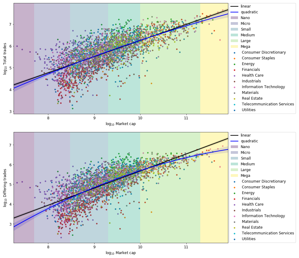
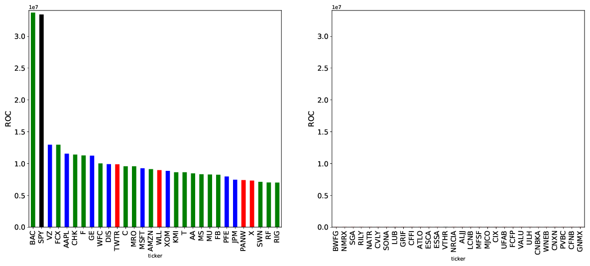
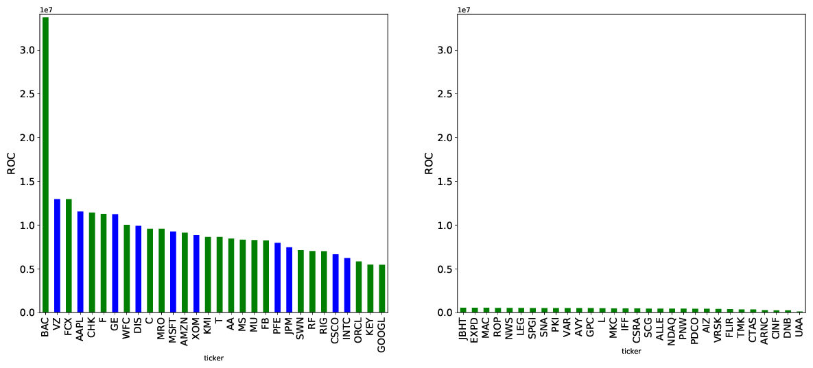
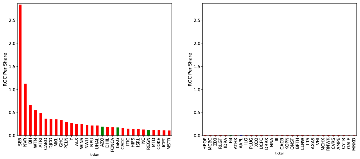
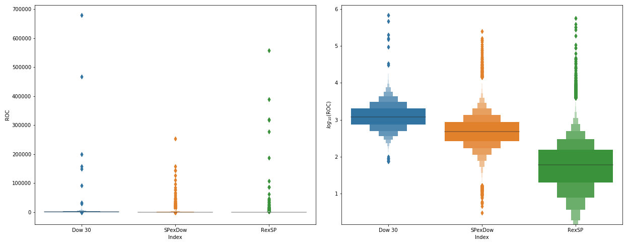
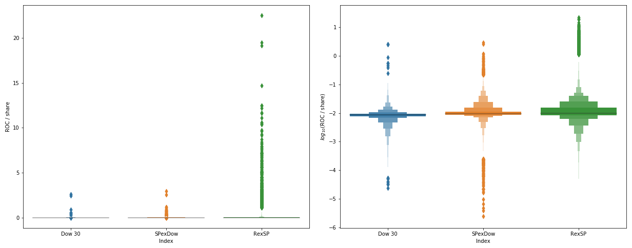
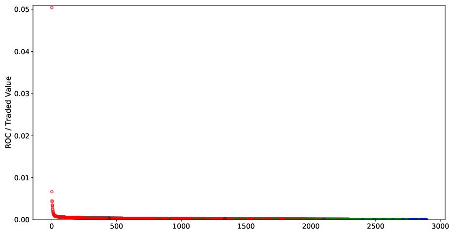
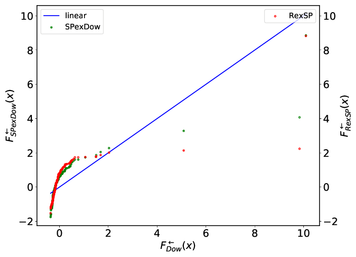
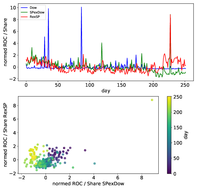
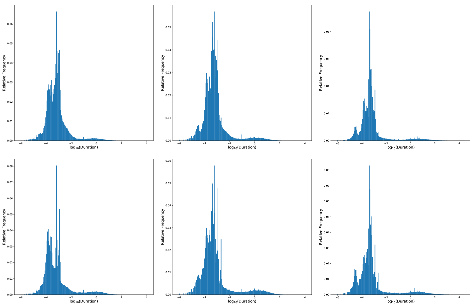
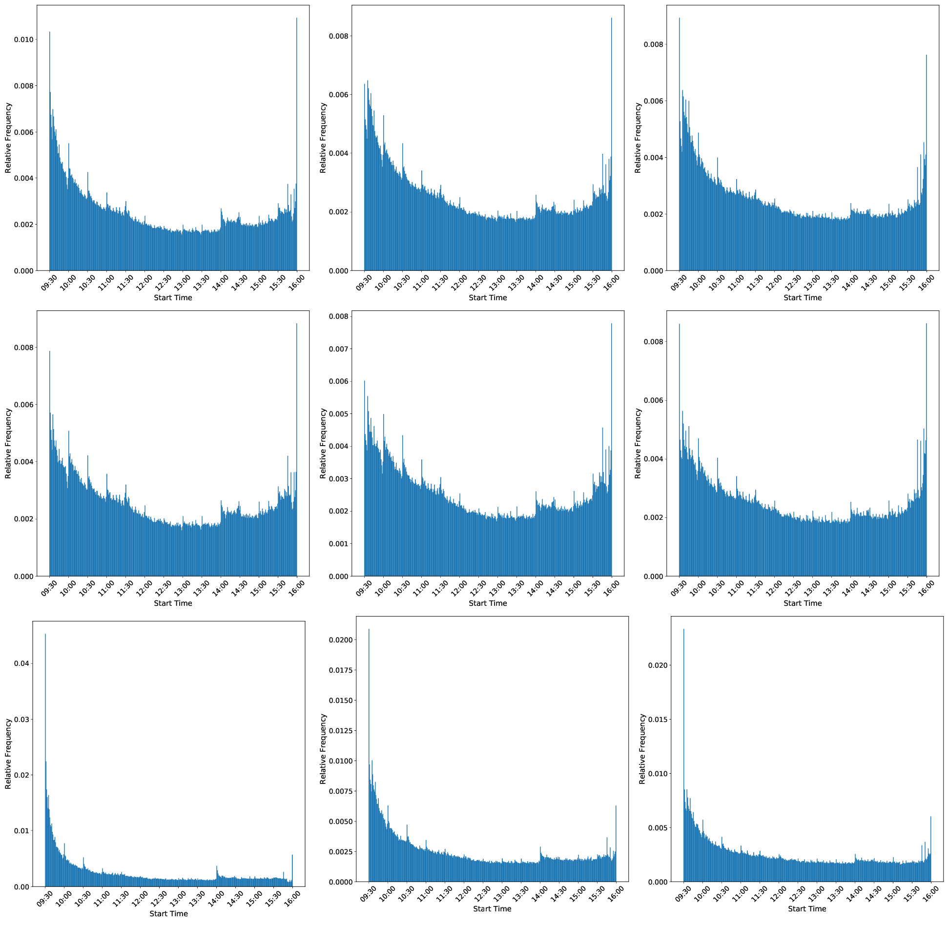
10 Statistics
Granger causality results for pairwise combinations of mutually-exclusive market category under study. Statistical significance was assessed using four Granger causality tests (parameter -test, sum of squared residuals -test, likelihood-ratio test, -test). Each causal relationship was considered significant if each of the four tests resulted in a -value less than . The maximum number of lags investigated was . Ordered pair Lags Dow RexSP 2, 3, 4, 13, 14, 15, 20, 22, …, 37 Dow SPexDow SPexDow Dow 1, …, 10, 15,…,24, 26, 30, …, 34 SPexDow RexSP 1, 2, 3, 4 RexSP Dow 1, 3, 35, 36 RexSP SPexDow
Ordinary least squares regression predicting realized opportunity cost (ROC) using market capitalization, differing trades, and total trades. Dep. Variable: ROC R-squared: 0.908 Model: OLS Adj. R-squared: 0.908 Method: Least Squares F-statistic: 7179. No. Observations: 2884 Prob (F-statistic): 0.00 Df Residuals: 2880 Log-Likelihood: 551.07 Df Model: 3 AIC: -1094. BIC: -1070. Omnibus: 1630.431 Durbin-Watson: 2.007 Prob(Omnibus): 0.000 Jarque-Bera (JB): 23812.396 Skew: 2.375 Prob(JB): 0.00 Kurtosis: 16.252 Cond. No. 259. coef std err z Pz [0.025 0.975] Intercept 1.0052 0.091 11.050 0.000 0.827 1.183 l_MarketCap 0.1183 0.011 10.675 0.000 0.097 0.140 l_total_trades -0.2203 0.043 -5.127 0.000 -0.304 -0.136 l_differing_trades 0.9023 0.040 22.286 0.000 0.823 0.982
Ordinary least squares regression predicting realized opportunity cost (ROC) using market capitalization, differing trades, and total trades. Quadratic terms are included. Dep. Variable: ROC R-squared: 0.925 Model: OLS Adj. R-squared: 0.925 Method: Least Squares F-statistic: 5970. No. Observations: 2884 Prob (F-statistic): 0.00 Df Residuals: 2877 Log-Likelihood: 846.73 Df Model: 6 AIC: -1679. BIC: -1638. Omnibus: 1952.210 Durbin-Watson: 1.988 Prob(Omnibus): 0.000 Jarque-Bera (JB): 50808.169 Skew: 2.831 Prob(JB): 0.00 Kurtosis: 22.768 Cond. No. 1.70e+04
| coef | std err | z | Pz | [0.025 | 0.975] | |
|---|---|---|---|---|---|---|
| Intercept | 7.8666 | 0.802 | 9.811 | 0.000 | 6.295 | 9.438 |
| l_MarketCap | -0.0738 | 0.149 | -0.496 | 0.620 | -0.365 | 0.218 |
| l_total_trades | -4.1661 | 0.432 | -9.638 | 0.000 | -5.013 | -3.319 |
| l_differing_trades | 3.0804 | 0.338 | 9.103 | 0.000 | 2.417 | 3.744 |
| l_MarketCap ** 2 | 0.0067 | 0.008 | 0.837 | 0.402 | -0.009 | 0.022 |
| l_total_trades ** 2 | 0.3385 | 0.038 | 8.936 | 0.000 | 0.264 | 0.413 |
| l_differing_trades ** 2 | -0.2042 | 0.034 | -6.002 | 0.000 | -0.271 | -0.138 |
Ordinary least squares regression predicting realized opportunity cost (ROC) using only market capitalization. Dep. Variable: ROC R-squared: 0.600 Model: OLS Adj. R-squared: 0.600 Method: Least Squares F-statistic: 4280. No. Observations: 2884 Prob (F-statistic): 0.00 Df Residuals: 2882 Log-Likelihood: -1574.9 Df Model: 1 AIC: 3154. BIC: 3166. Omnibus: 52.492 Durbin-Watson: 1.933 Prob(Omnibus): 0.000 Jarque-Bera (JB): 76.592 Skew: 0.199 Prob(JB): 2.34e-17 Kurtosis: 3.692 Cond. No. 126. coef std err z Pz [0.025 0.975] Intercept -1.4415 0.108 -13.398 0.000 -1.652 -1.231 l_MarketCap 0.7368 0.011 65.422 0.000 0.715 0.759
Ordinary least squares regression predicting realized opportunity cost (ROC) using only market capitalization. Quadratic terms are included. Dep. Variable: ROC R-squared: 0.603 Model: OLS Adj. R-squared: 0.603 Method: Least Squares F-statistic: 2904. No. Observations: 2884 Prob (F-statistic): 0.00 Df Residuals: 2881 Log-Likelihood: -1564.7 Df Model: 2 AIC: 3135. BIC: 3153. Omnibus: 67.584 Durbin-Watson: 1.935 Prob(Omnibus): 0.000 Jarque-Bera (JB): 100.782 Skew: 0.242 Prob(JB): 1.30e-22 Kurtosis: 3.777 Cond. No. 1.24e+04 coef std err z Pz [0.025 0.975] Intercept -6.2441 1.286 -4.857 0.000 -8.764 -3.724 l_MarketCap 1.7575 0.266 6.598 0.000 1.235 2.280 l_MarketCap ** 2 -0.0539 0.014 -3.927 0.000 -0.081 -0.027