Binary Stochastic Filtering: a Method for Neural Network Size Minimization and Supervised Feature Selection

Abstract

Binary Stochastic Filtering (BSF), the algorithm for feature selection and neuron pruning is proposed in this work. The method defines filtering layer which penalizes amount of the information involved in the training process. This information could be the input data or output of the previous layer, which directly lead to the feature selection or neuron pruning respectively, producing ad hoc subset of features or selecting optimal number of neurons in each layer.

Filtering layer stochastically passes or drops features based on individual weights, which are tuned with standard backpropagation algorithm during the training process. Multifold decrease of neural network size has been achieved in the experiments. Besides, the method was able to select minimal number of features, surpassing literature references by the accuracy/dimensionality ratio.

Ready-to-use implementation of the BSF layer is provided.

Keywords: Feature selection; dimensionality reduction; neural network; neuron pruning

1 Introduction

Supervised learning algorithms rely on prearranged labeled datasets as a source of information. In a variety of cases a dataset consists of a significant number of various features (e.g. versatile statistical measures for text or network data processing), with only some of them containing sensible information for solving given problem (usually classification or regression). The process of finding an information-rich subset is called feature selection and is of growing interest during modern development of machine learning. Correct feature selection aims to reduce the computational complexity, to enhance generalization [1] or may be of interest on its own for further interpretation.

Figure 1: Number of publications considering feature selection in past years. Image is generated based on data from the Web of Science service [2], searched for topic: “feature selection”.

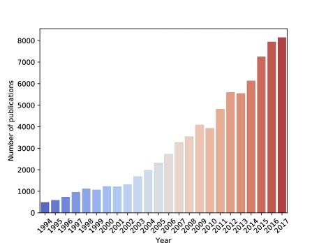
Numerous approaches were proposed in the last 25 years (Fig. 1), which include algorithms based on information theory, that tries to estimate the amount of information, brought to the dataset by a given feature [3, 4, 5], Relief and derived algorithms [6, 7], based on nearest neighbor search, statistical [8] and spectral graph theory based [9], etc. The very modern approaches are mainly focused on the application of swarm intelligence algorithms [10, 11, 12] Nevertheless, different methods usually lead to strongly discrepant sets of features and final decision could be made only after a series of experiments.

This paper proposes in situ feature selection method which relies on the intrinsic optimization algorithms, used in machine learning without any external entities. Filtering layer performs search for least possible feature involvement by minimization of feature passing probabilities. Furthermore, filtering may be utilized for neuron or kernel pruning, minimizing the size of a network similarly to features, which leads to multifold increase of NN performance. The method can be applied to different kinds of NN, optimized for various datasets, which is demonstrated in this work.

2 Method

Stochastic neurons, the units with nondeterministic behavior are known for a long time, at least since mid 1980s, when Boltzmann machines became popular [13]. Besides, the stochastic neurons are of interest because of their closeness to the biological ones [14]. The successful networks, consisting of stochastic neurons were built [15]. Nevertheless, mixing of stochastic and deterministic units in one network is not common, except for Dropout technique [16], which works by randomly disabling deterministic neurons to prevent overfitting.

The proposed algorithm is inspired by both stochastic neurons and dropout. The method combines two ideas mentioned above and could be thought as a generalization of dropout with trainable individual dropout rates, or as incorporation of the special version of stochastic neurons into classical deep NN structure. Proposed binary stochastic filtering (BSF) method works by setting the BSF layer (consisting of the BSF units) after the layer, outputs of which are to be filtered. BSF unit stochastically passes the input without changes or sets it to zero with probabilities based on the unit weights. Strictly speaking, BSF unit is described as:

$$BSF(x,w,z)=x_{z<w}$$ (1)

where $w$ represents the adjustable weight of a given unit and $z$ is uniformly sampled from the range $[0,1]$. This definition is inspired by the formula from the work of Bengio et al. ([17], Eq. (3)). Authors have defined the Stochastic Binary Neuron as $h_{i}=f(a_{i},z_{i})=1_{z_{i}>sigm(a_{i})}$, where neuron activation $a_{i}$ is given as a weighted sum of its inputs. This definition is directly derived from the classical deterministic neurons and could be thought as a noisy modification of them. In contrast, BSF includes the single input which passes through the unit if random value $z$ is smaller than weight $w$ or nullified instead. Thus, probability of output to be $x$ is equal to the probability of $z$ to be less than $w$, $\mathbb{P}(x)=\mathbb{P}(z<w)$, which is equal to $F_{z}(w)$, where $F_{z}$ is a cumulative distribution function for the variable $z$. From the properties of uniform distribution,

$$F_{z}(w)=\begin{cases}0,&\text{$\mbox{for}\ w<0$}\\ {w-a}\over{b-a},&\text{$\mbox{for}\ w\in[a,b)$}\\ 1,&\text{$\mbox{for}\ w\geq 0$}\end{cases}$$ (2)

on the interval $[a,b]$ from which $z$ is sampled, $F_{z}(w)=w$, as $[a,b]=[0,1]$. In other words, BSF multiplies the input by random variable $b$, sampled from Bernoulli distribution with parameter equal to the unit weight $w$:

$$BSF(x,w)=x\cdot b,\leavevmode\nobreak\ b\sim Bernoulli(w)\$$ (3)

This allows selective filtering of the layer inputs with adjustable probabilities of the given input to be filtered, which equals the weight $w$, supposing $w\in[0,1]$. Setting $w$ to be close to 0 means that the given feature is close to being completely filtered out, while in case of $w$ being close to 1, feature passes through BSF without changes. Thereby, by tuning the BSF layer weights it is possible to control how much each of the features participates in the training process.

From the obvious reasons, the gradient of a stochastic unit is stochastic as well, being equal to zero or $\infty$ randomly. Thus, backpropagation training, being a variation of gradient descent method is not able to optimize weights of the BSF units. G. E. Hinton has suggested a straight through (ST) estimator [18], which defines the gradient of stochastic unit with respect to its input $\frac{\partial BSF(x)}{\partial x}=1$. Few modifications of this approach were reported, such as multiplication of the gradient by a logistic sigmoid derivative, i.e. $\frac{\partial BSF(x)}{\partial x}=\frac{{d\sigma(x)}}{dx}$, where $\sigma(x)={1\over 1+e^{-x}}$ but it was found that simpler unity gradient achieves better performance [17] as it does not suffer from vanishing gradients issue. ST estimator is especially suitable when stochastic neurons are mixed with normal ones, as it does not distort the gradient between classical units. Proof of the last statement is given in the Appendix 8.

Thus, by applying the ST estimator, weights of BSF layers could be optimized during model training. Moreover, penalizing of the filter weights will lead to a decrease of above-lying layer involvement in the NN working process, which could be used for neuron pruning or overfitting prevention. Placing the penalized BSF layer as the input layer of the NN will decrease probabilities of feature occurring in correspondence to their importance, which is equivalent to the feature selection.

2.1 Feature selection

2.1.1 Deep NN classifier

Figure 2: Structure of classical multilayer perceptron (left) and same network with included BSF layer. Deterministic and BSF units are drawn in circles and squares respectively, $v_{1..3}$ correspond to input features.

Classifier is a model, performing mapping from n-dimensional data space $D^{n}\rightarrow L$ to the label space consisting of finite (and usually relatively low) number of labels. As a deep NN classifier, a classical multilayer perceptron model with softmax activation of the output layer was used [19]. Softmax function is a generalization of logistic function for a multilabel classification problem, defined as

$$\sigma_{i}(\vec{x})=\frac{{e^{x_{i}}}}{\sum_{j=1}^{N}{e^{x_{j}}}}$$ (4)

for $i=1,2,...,N$ where $N$ describes number of classes in a given problem. Unlike classical binary logistic regression, which outputs the scalar probability $p$ of a data to be true and $1-p$ to be false, softmax function outputs a vector $\vec{{p}}$ with length $N$, each element of which represents the probability of the input sample to belong to each of the classes. Normalization by the sum of outputs guarantees that total probability of a sample to belong to all classes will always be unity. Exploitation of the softmax function needs label to be one hot encoded, i.e. to the vector with length $N$

$$L_{oh}(i)=\begin{cases}1,&\text{if $i=classindex$}\\ 0,&\text{elsewhere}\end{cases}$$ (5)

In that case loss function must describe divergence between $\vec{{p}}$ and encoded label $\vec{{L_{oh}}}$, i.e. maps two vectors to a scalar. Cross-entropy, a function derived from the maximum likelihood estimation method is widely used as a loss [20]. The function is defined as

$$E=-\sum_{i=1}^{N}{c_{i}\cdot ln(p_{i})+(1-c_{i})\cdot ln(1-p_{i})}$$ (6)

where $c_{i}$ is the actual class label and $p_{i}$ is corresponding element of $\vec{{p}}$. The selected NN model consists of 4 layers with rectified linear activation [21] in the hidden layers. Number of units in each layer was empirically chosen as $D$, $D$, $2D$, $D$, $N$ respectively, where $D$ is the dimensionality of input data, in order to meet the different number of features in used datasets. The model was optimized using Adam algorithm [22] with parameters $\alpha=0.001$, $\beta_{1}=0.9$, $\beta_{2}=0.999$, as it is specified in the original paper with zero learning rate decay. The same optimizer was used for training of all other models.

Classification accuracy for every dataset was estimated using 10-fold cross-validation method. The NN was trained until full convergence (no loss decrease), both training and validation mean accuracies were used for evaluation of model performance.

Binary stochastic filter was placed as an input layer to the NN of the same structure as classifier, resulting in 5 layer network. $L_{1}$ regularization was used as a penalty, with the regularization coefficient defining the tendency of the data to be filtered out. Generally, this coefficient serves as a metaparameter in the filtering layer, and needs to be adjusted to meet the classifier loss. Good results were achieved with regularization coefficient lying in the range 0.001-0.05. The examples of training process visualization depending on the regularization rate are provided in the supplementary materials. The model was trained until convergence. After model fitting, weights of a BSF layer were analyzed and treated as a feature importances. The highest importance features were manually selected and saved forming a reduced dataset. Afterward, normal classifier was trained as described above for estimation of classification accuracy for the reduced dataset. To estimate changes in high-dimensional cluster separation, the simple and well-known silhouettes method [23] was used. In brief, the method defines silhouette $s(i)$ which compares mean inter-cluster distance $a(i)$ for the given data point $i$ and mean distance to all objects belonging to the nearest cluster $b(i)$.

$$s(i)=\frac{b(i)-a(i)}{max\{a(i),b(i)\}}$$ (7)

The mean value of silhouettes (silhouette coefficient) for all the datapoints within dataset is a measure for cluster separation, lying in the range $[-1,1]$ where higher number means better separation.

(a)

Figure 3: (a) Weights of the BSF layer after fitting MNIST dataset. (b) Set of Raman spectra of different classes after normalization. (c) Regions of interest of the spectra selected by BSF.

(b)    (c)

2.1.2 Convolutional NN classifier

Convolutional NN (CNN) makes use of data spatial independence, which is especially useful in image recognition. The CNN architecture was proposed by Le Cun et al. [24] for number recognition problems. Generally, architecture implements discrete convolution operation, which converts input data (image) to the feature maps. Convolution kernel is optimized during the training process to minimize the loss function value. Produced maps of features are convoluted further, producing higher-order maps. After few subsequent convolutional layers the classical fully-connected classifier (described in the previous part) is placed, which performs actual classification [25].

The CNN classifier with structure, described in the Table 6, was implemented in the experiments. Its architecture resembles typical simple CNNs, widely used in for educational and research purposes. First 3 layers form the convolutional block, which performs feature extraction from images, while 3 last layers correspond to the fully-connected classifier. The model was trained in the same manner as the DNN classifier described in the previous part (Subsection 2.1.1).

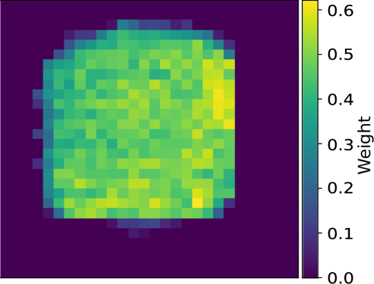
Interpretation of feature selection results for image recognition problem is not that straightforward in comparison to the simple perceptron classifier, as the convolution operations need input data to maintain well-defined shape. Nevertheless, its patterns, being visualized, are easily recognizable. In that case, BSF provides attention maps, i.e. highlights the regions of images with the highest information density, averaged over whole dataset.

2.1.3 Spectra recognition

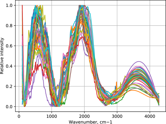
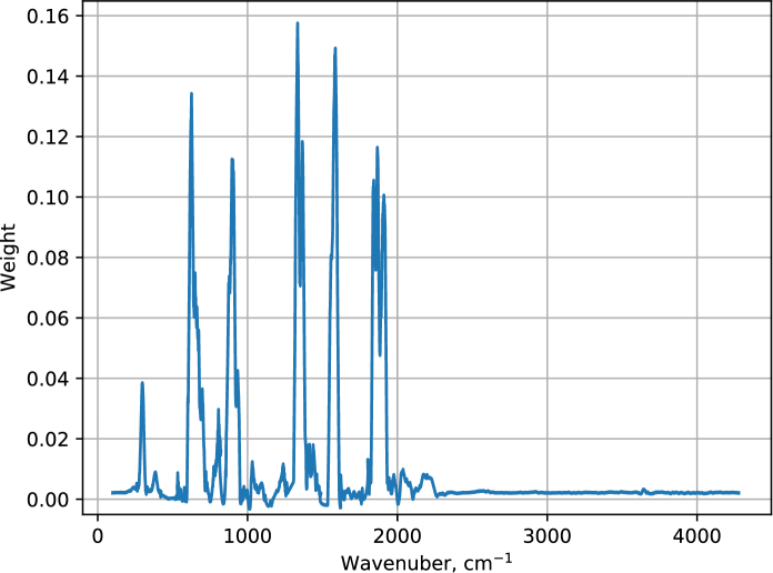
The interpretation of complex compounds spectra is a known problem in analytical chemistry. This kind of data contains information about characteristic vibrations of molecules, encoding its structure. Classically, spectra are manually analyzed by chemists, taking into account shape and position of spectral peaks. Due to the finite resolution of the spectroscopes, if a large number of peaks are present (i.e. for complex molecules) peaks overlap and interfere, making spectra impossible to interpret by human. Few reports on the successful use of machine learning techniques for identification of the biological samples were published [26, 27]. The binary stochastic filter was formulated during work on a similar problem, the classification of DNA spectra. Such spectra are not readable by human due to presence of thousands of different vibration frequencies. Spectra were classified by the CNN model consisting of 3 convolutional and 4 fully-connected layers with satisfactory results. After that, binary stochastic filter layer was added to the model input and training process was repeated. Weights of the BSF layer, in that case, correspond to the spectral regions of interest. Weights of the layer were visualized (Fig. 3a (b)) and treated as regions of interest of spectra. Correspondence between them and expected vibrational frequencies of the DNA constituents [28] were observed. This method allows obtaining information about chemical changes in a set of similar compounds or mixtures, spectra of which are indistinguishable by other methods.

2.2 Neuron pruning

Sparse neural networks are believed to be more efficient than popular fully-connected systems due to enhanced generalization, faster convergence and higher performance [29]. An alternative way to sparsifying is neuron pruning, the removal of the least important units from the network, which was demonstrated by Mozer and Smolensky [30]. The latter approach seems to be more beneficial from the performance point of view as removal of the single unit leads to the greater decrease of computational complexity, nevertheless the former became more frequent, being popularized by the above-mentioned work of Le Cun [29]. Furthermore, the analysis of units importance is less complex because of their significantly lower amount in comparison to weights.

Figure 4: Neuron pruning algorithm graphical summary

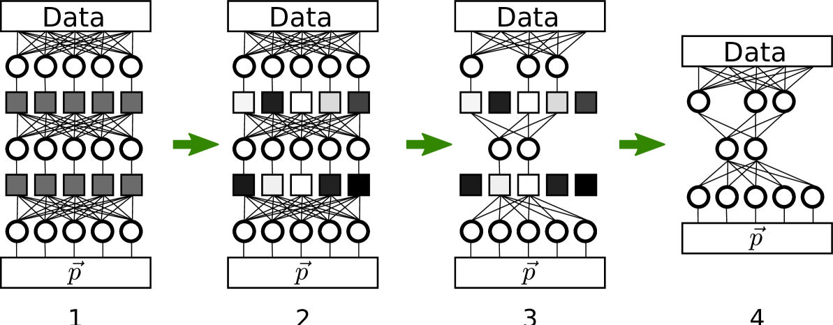
By placing binary stochastic filter between NN layers it is possible to disable the least important parts during training process. Applying the BSF unit to every interunit connection may be used to prune specific weights while applying it to the output of above-laying unit will cause neuron pruning. The second approach was selected according to above-described reasons and straightforward implementation. The algorithm is schematically shown in the Figure 4.

1. The fully-connected model with excess units is built, and BSF units (drawn as squares) are placed after each dense layer.

2. During training process the weights of neurons and BSF are optimized (values of BSF units are visualized as lightness of the squares, i.e. dark values correspond to lower weights)

3. Weights of the filter are analyzed and neurons corresponding to the low weights are deleted.

4. The BSF layers are removed leaving the shape-optimized and trained NN model which could be additionally trained for fine-tuning.

2.3 Kernel pruning

Modern convolutional networks frequently contain tens of layers, having hundreds of convolutional kernels. For example, ResNet image recognition network [31] is composed from 34 layers having up to 512 convolutional kernels. This makes such networks extremely computationally intractable for both training and evaluation, limiting their applications to hardware-accelerated desktops or servers, leaving aside highly attractive embedded and mobile systems. This issue could be solved by finding reduced number convolution kernels, enough to maintain the classification accuracy. This could be done with slightly modified version of BSFilter, which filters out feature maps, produced by convolution operation, instead of a single neurons. Otherwise, the method is similar to the described in the previous subsection.

2.4 Implementation

The BSF layer was implemented in Keras framework with Tensorflow back-end [32, 33] based on above-discussed theory. Implementation together with usage instructions is available on GitHub . All NN models used in experiments were built by dint of the same framework.

3 Results

Three different datasets were used, the Wine dataset [34], KDD-99 [35] and Musk2 dataset [36]. As an original KDD99 dataset is huge (around 5 million of instances), a sample of around 1 million instances was used instead. The datasets summary is given in the Table 1.

Table 1: Classification datasets summary

	Instances	Classes	Features	Description
Wine	178	3	13	Chemical analysis of a wine from three different cultivars
KDD99	918455	21	41	Wide variety of intrusions data simulated in a military network environment.
Musk2	6598	2	168	Conformation of molecules judged to be musk or non-musk

Datasets were standardized by removing mean and scaling to unit variance. Musk2 and KDD99 datasets contain categorical data labels which were encoded as integers before standardization.

3.1 Deep NN classifier

NN classifier was trained on each dataset and corresponding accuracies were saved as original. Feature selection was performed as it is described in the Subsection 2.1.1, and accuracy estimation was repeated for truncated versions of datasets. Obtained data is summarized in the Table 2 together with reference accuracies, found in the literature. Additionally, the experiment was repeated for KDD99 dataset but with 12 least important features (corresponding BSF weights are below 30th percentile). Maximal accuracy has achieved 57.82 % in that case.

The implementation of silhouettes from the scikit-learn project [37] was used in the experiment. The method was applied to the original and truncated versions of the Wine dataset. Silhouettes coefficients (2) for these datasets were calculated as 0.2798 and 0.3785 respectively, which is an evidence of enhanced cluster separation after feature selection.

Stability of a binary filter was estimated by varying the structure of NN classifier, training the system with KDD99 dataset and analyzing the features of the highest importance (above 80th percentile). Each experiment was repeated 4 times and selected features were summarized in the Table 7. The column NN structure contains the number of units in each layer and their activation functions. Additionally, the output of every model consists of a softmax-activated layer, which is not shown in the table.

Table 2: Comparison of classification results for original and truncated versions of three given datasets (cross-validated)

	Wine	KDD99	Musk2
Training accuracy, original	1.000	0.9993	1.000
Validation accuracy, original	0.9891	0.9993	0.9066
Number of selected features	6	8	42
Training accuracy, truncated	1.000	0.9975	1.000
Validation accuracy, truncated	0.9889	0.9975	0.9251
Reference accuracy	0.9887 [38]	0.9941 [39]	0.8920 [36]

3.2 Convolutional Classifier

The MNIST dataset from the work of Le Cun et al. [24] was used for CNN training. The original set contains 60000 handwritten digit images of size 28x28 pixels with labels, from which 15000 were randomly sampled as training dataset and another 5000 as validation one. The implemented model structure is shown in the appendix (Table 6). The model has achieved training and validation accuracies of 1.000 and 0.990 respectively. BSF layer was added to model and training process was repeated. The weights of the layer were visualized (Fig. 3a (a)) and clearly correspond to the central part of the image where the majority of information about the digit is located. An animated demonstration of the training process could be found in supplementary materials.

3.2.1 Spectra recognition

A classifier model was trained on spectra dataset, a sample of which is shown in Fig. 3a (b). Weights of the layer are then visualized (Fig. 3a (c)) and treated as regions of interest of spectra.

3.3 Neuron pruning

The experiment was performed with the datasets, used in the Section 2.1.1. The implementation utilizes additional functions for model rebuilding [40]. The model with excess neurons was trained on each dataset until convergence and then pruned. The weights of the shape-optimized model were reset and model was trained until convergence (number of epochs were determined experimentally to guarantee no further loss decrease) in 10-fold cross-validation manner,

Mean values for accuracy are tabulated in the Table 3.

Table 3: Summary of the NN pruning results for different datasets and corresponding accuracies

	Wine	KDD99	Musk2
Training accuracy, original	1.000	0.9993	1.000
Validation accuracy, original	0.9891	0.9993	0.9066
Original number of units/weights	56/953	185/9430	666/138778
Number of units/weights after pruning	33/469	31/595	57/4103
Training accuracy, pruned	1.000	0.9993	1.000
Validation accuracy, original	0.9830	0.9993	0.9987

3.4 Kernel pruning

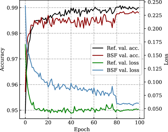
Two datasets were used in the experiments, above-mentioned MNIST and CIFAR10, containing 60000 32x32 images, grouped into 10 categories [41]. Due to the significant difference between datasets, two convolutional models have been used. The MNIST dataset was classified with the same CNN as described in section 3.2. CIFAR10 dataset was classified with simple deep CNN, described in Keras documentation [42]. In the first stage, both datasets were classified by training for $N_{tr}$ epochs and then fine-tuned by additional training for $N_{ft}$ epochs with optimizer, learning rate of which was reduced in 10 times. In the second stage, the modified BSFilter layer was placed after each of the convolutional layers, the model was trained by the same number of epochs, pruned and fine-tuned for $N_{ft}$ epochs.

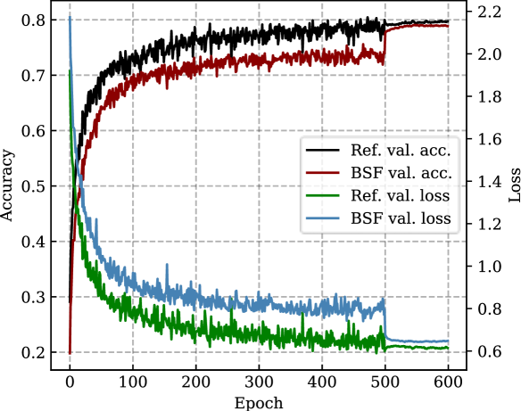
Validation accuracy and loss evolution during training for both datasets is presented in the Figure 5. Final accuracies, losses, number of weights and model size are tabulated in the Table 4.

(a)

(b)

Figure 5: Validation accuracy and loss evolution during CNN models training for CIFAR10 (a) and MNIST (b) datasets. Change of curve behavior at after 500^th epoch (a) and after 80^th epoch (b) is connected with change of learning rate and model pruning.

Model	L1 coef.	Accuracy	Loss	Weights	Size
MNIST	—	0.9900	0.0488	1,199,882	13.8 MiB
MNIST+BSF	$1\text{\times}{10}^{-3}$	0.9880	0.0600	279,508	3.2 MiB
MNIST+BSF	$1\text{\times}{10}^{-2}$	0.9818	0.1131	112,144	1.3 MiB
CIFAR10	—	0.7972	0.6143	1,250,858	9.6 MiB
CIFAR10+BSF	$1\text{\times}{10}^{-4}$	0.7885	0.6479	391,519	3.1 MiB
CIFAR10+BSF	$1\text{\times}{10}^{-3}$	0.7583	0.7277	269,273	2.1 MiB

Table 4: Summary of kernel pruning results. Accuracy and loss values obtained from the validation run.

4 Discussion

4.1 Deep NN classifier

From the classification results (Table 2) one can conclude that correct feature selection may lead to significant increase of model performance without considerable loss of accuracy, as for each of three datasets the multifold dimensionality decrease was observed, leading to the corresponding reduction of computational complexity. Experiment with features corresponding to the lowest BSF weights proves that these features do not contain important information for classification.

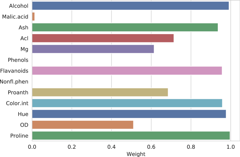
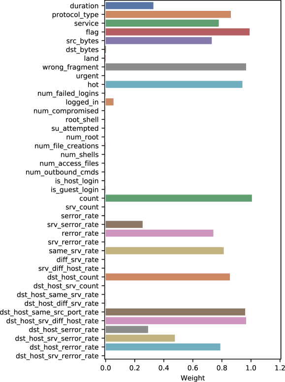
Another important consequence is the fact that BSF allows concluding which features in the dataset actually carry information. The importance distribution for two datasets (Wine and KDD99) is shown in the Appendix. It is possible to conclude that some of the data, present in datasets is not meaningful in the classification problem, i.e. does not contain information about belonging to some class, like phenols concentration in Italian wines (Fig. 9) or number of accessed files in the malware traffic (Fig. 10). This could lead to interesting conclusions, like independence of phenols concentration on used cultivar. The Musk2 dataset is not easily interpretable in a similar style, but the results could probably be even more important, as from the meaningful features the information about molecule biologically active sides could be extracted, which may be the valuable information for drug designers.

Because of the high popularity of KDD99 dataset, it is possible to additionally compare feature selection results with results of other researchers, which are tabulated in the Table 5. In addition to 8 selected features, mentioned above, the truncated dataset was enlarged to 14 features, which is the minimal dimensionality leading to zero decrease of accuracy in comparison to the original dataset. It is possible to conclude from the table, that BSF surpasses other feature selection methods in terms of accuracy per number of features. It is worth mentioning that in the works used for comparison, best Validation accuracy was used as a measure of classification success, while present work uses the cross-validated average accuracy.

Table 5: Comparison of feature selection results for KDD99 dataset

Method	Features	Accuracy	Reference
Fast correlation-based filtering, Naive Bayes/decision tree	12	0.9460	[43]
Decision tree, simulated annealing	28	0.9936	[44]
Support vector machine, particle swarm optimization	26	0.9945	[45]
Supported vector machine, simulated annealing	25	0.9942	[46]
Supported vector machine, decision tree, simulated annealing	23	0.9996	[44]
Binary stochastic filtering	8	0.9975	-
Binary stochastic filtering	14	0.9993	-

(a)

(b)

Figure 6: Visual representation of the (a) original Wine dataset and (b) its truncated version, containing 6 most important features. It is visible that cluster separation has increased after removing unimportant features. Data was compressed to 2 dimensions by the T-SNE algorithm.

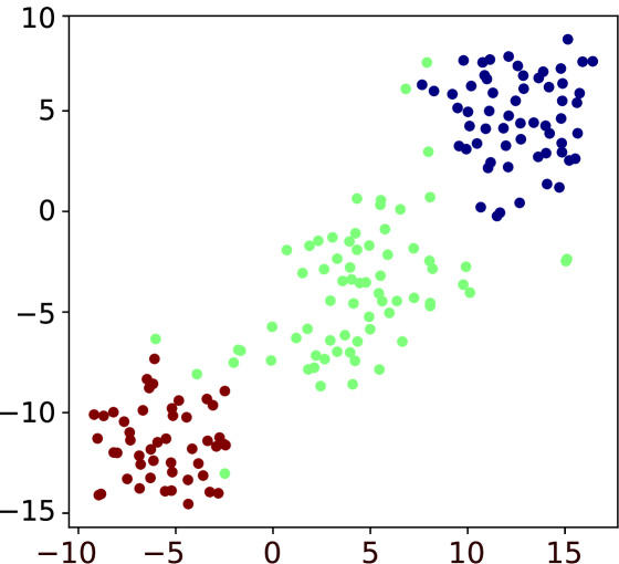
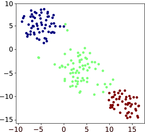
Values of silhouettes coefficient for the truncated Wine dataset were observed to be higher than for original version. Thus, removing unimportant features, that behave as noise, actually improves the dataset classification. Both versions were additionally processed with the well-known T-SNE algorithm [47], which allows high-dimensional data visualizing in the two-dimensional plot, which makes it possible to see enhanced separation by naked eye. Generated images are shown in the Fig. 6

The stability estimating experiments demonstrate the fact that the BSF feature selector is relatively stable with only a small portion of features changing in different experiments. It was found by manual observation of selected features importances, that differences in selections occurs from the threshold separation into important and unimportant. During selection, weights of some features are approaching unity, while other ones are approaching zero. Stochastic nature of selection process causes small deviations in the weights of most important features ($w\approx 1$), which leads to fluctuations in selection results. This could be observed in the animation visualizing the BSF weights evolution during training process available in the supplementary materials.

4.1.1 Spectra recognition

Good correspondence between high-weight areas, threated as regions of interest and vibrational frequencies of the DNA constituents [28] was observed, which was expected from the chemical point of view. This method allows one to obtain information about subtle chemical changes in difficult samples.

4.2 Self-optimizing neural network

Minimal decrease of accuracy was observed from the data, given in the Table 3, while number of weights was reduced significantly, from 2 to approximately 34 times. This corresponds to the enhancement of performance for NN prediction of the same order, as computational complexity is directly connected to the number of weights. Such optimization could be especially beneficial for the embedded NN applications having limited computational resources. Obviously, the scale of NN pruning depends on initial redundancy but from the experiments it is possible to make empirical remark that satisfactory starting number of neurons in the hidden layers is equal to the dimensionality of input data. Another important outcome is the fact that Musk2 dataset, which was the most efficiently pruned, exhibits a considerable increase of Validation accuracy, i.e. improved generalization in correspondence with the [29]. Obtained cross-validated accuracy (0.9987) exceeds all experimental accuracies for the given dataset, found in literature (0.8920, 0.8333, 0.9600) [36, 48, 49].

4.3 Kernel pruning

(a)

(b)

Figure 7: Images, maximizing activation of the last convolutional layer for pruned CNN (a) and original CNN (b). For the latter, 16 images were randomly selected from the total of 64.

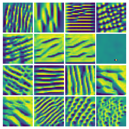
Results, summarized in the Table 4 demonstrate that kernel filtering with successive pruning is able to significantly decrease computational complexity of the image-recognition CNN at the price of minor accuracy drop. Precisely, more than threefold decrease in number of weights for the CIFAR10 dataset was achieved, accompanied by a change in accuracy by less than 1 %. Stronger penalization of the BSF layer lead to even more significant pruning, leaving around 20 % from the initial network weights. Nevertheless, in that case the decrease in accuracy was around 4 %, which is unacceptable. This observation may be used as an indicator of the optimal number of weights in the network.

During experiments with MNIST dataset, the number of weights was reduced in 4.3 times with change of accuracy in 0.2 %. In the experiments with increased penalization coefficient more than tenfold reduce in weights was reached at the cost of accuracy decrease by 0.82 %.

From the results above follows the fact that efficiency of kernel pruning (same as neuron pruning) strongly depends on the initial redundancy of neural network. By tuning penalization coefficient and observing the change of accuracy and loss it is possible to find the optimal balance between size of the CNN and its predictive ability.

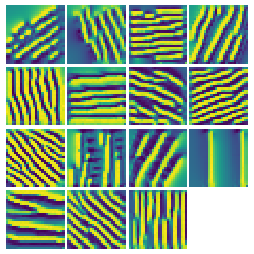
Other interesting conclusions could be done from the analysis of the convolutional kernels, optimized during CNN training. To visualize convolutions the input images, maximizing activation of a given kernel were generated with keras-vis library [50]. This method was applied to the last convolutional layer of the MNIST classifier, having 64 kernels in the original model and 15 in the pruned version. Results, presented in the Figure 7 demonstrates that pruned model is prone to learn smaller number of simpler kernels, mostly differently inclined lines, which encode majority of the information about the number. Unconstrained original model learns more complex patterns, such as curves, crosses and others which are difficult to interpret by a human, representing less informative details of the image. This gives a clue to the question of how the majority of kernels could be removed from the model almost without drop in generalization: the CNN is focused on the most informative features, ignoring the details.

5 Conclusion

Binary stochastic filter is a straightforward method for estimating importances of input features or specific units. In comparison to existing works, which select features by repetitive evaluating performance of subset, BSF works in situ with the whole dataset, minimizing feature involvement in the training process. The method has a wide variety of possible applications, including feature selection and NN size minimization. Thank its layered structure it can be easily introduced to different kinds of NN without any additional overhead. During experiments, BSF selected 8 features from 42 in the KDD99 dataset, bearing enough information for close-to-one prediction accuracy. Such kind of feature selection is of interest in natural sciences, as with its help one could make conclusions about processes, generating information, contained in dataset. Suggested neuron pruning algorithm has led to a significant increase of NN performance in experiments, decreasing the number of weights in $\approx$34 times for Musk2 dataset. What even more substantial, after shape optimization 10-fold crossvalidation test demonstrated considerable increase of validation accuracy, proving better generalization. Kernel pruning, implemented with BSF has achieved more than tenfold decrease of model size, which makes it a promising method for transferring NN to the mobile and embedded systems.

Thus, BSF could become a useful tool in the different fields of machine learning. Further work will include investigation of the weights pruning, i.e. network sparsifying, generalizing of BSF layer for filtering convolution maps, i.e. kernel sparsifying and application of the method to more complex NN structures, such as adversarial networks and autoencoders.

Appendix A Proof of gradients independence on introducing BSF layer

(a)

(b)

Figure 8:

Proof.

Suppose the multilayer perceptron is given. Let us focus on the two hidden layers in the perceptron, having indices $l$ and $l+1$ and containing $i$ and $j$ neurons in each respectively (Fig. 8 (a)). Suppose the partial derivatives of loss function $L$ with respect to the neuron pre-activation $z_{j}^{l+1}$ is given. Let us call this value $\delta_{j}^{l+1}=\frac{\partial L}{\partial z_{j}^{l+1}}$ an error of the $j$ neuron in the $l+1$ layer, which could be computed from the classical backpropagation algorithm, and is enough for the computing of derivatives with respect to weights, as $\frac{\partial L}{\partial w_{ij}^{l-1}}=\frac{\partial L}{\partial z_{j}^{l+1}}\frac{\partial z_{j}^{l+1}}{\partial w_{ij}^{l+1}}$. Now the error of the neuron in $l$ layer could be calculated using chain rule as

$$\text{$\delta_{i}^{l}=$}\sum_{j}\frac{\partial L}{\partial z_{j}^{l+1}}\frac{\partial z_{j}^{l+1}}{\partial a_{i}^{l}}\frac{\partial a_{i}^{l}}{\partial z_{i}^{l}}$$ (8)

where $a_{i}^{l}$ stands for activation (output) of the $i$ neuron in $l$ layer. $\frac{dz_{j}^{l+1}}{\partial a_{i}^{l}}$ could be derived from the equation describing neuron, $z_{j}^{l+1}=\sum_{i}a_{i}^{l}w_{ij}^{l+1}+b_{j}^{l+1}$ ($w_{ij}^{l+1}$ corresponds to weight, connecting the $i^{th}$neuron from $l$ with $j^{th}$ neuron in $l+1$, $b_{j}^{l+1}$ to corresponding neuron bias). As activation $a_{i}^{l}$ is independent on other neurons in $l$ layer, the sum could be omitted. By differentiating:

$$\frac{\partial z_{j}^{l+1}}{\partial a_{i}^{l}}=w_{ij}^{l+1}$$ (9)

Last term $\frac{\partial a_{i}^{l}}{dz_{i}^{l}}$ could be derived at a similar manner, as $a_{i}^{l}=act(z_{i}^{l})$, where $act(z)$ is activation function,

$$\frac{\partial a_{i}^{l}}{\partial z_{i}^{l}}=act^{\prime}(z_{i}^{l})$$ (10)

Substituting 9 and 10 into 8, the equation for computing error of the neurons in $l$ layer could be obtained ($act^{\prime}(z_{i}^{l})$ is independent on indices of neurons in $l+1$ layer, so it could be factored out):

$$\text{$\delta_{i}^{l}=$}act^{\prime}(z_{i}^{l})\sum_{j}\delta_{j}^{l+1}w_{ij}^{l+1}$$ (11)

Now suppose a BSF layer is introduced in between two classical layers, as it shown in the Fig. 8 (b). Now numbering will be performed by indices $i$, $j$, $k$ for every consequent layer. Then

$$\text{$\delta_{i}^{l-1}=$}\sum_{k}\frac{\partial L}{\partial z_{k}^{l+1}}\frac{\partial z_{k}^{l+1}}{\partial a_{j}^{l}}\frac{\partial a_{j}^{l}}{\partial z_{j}^{l}}\frac{\partial z_{j}^{l}}{\partial a_{i}^{l-1}}\text{$\frac{\partial a_{i}^{l-1}}{\partial z_{i}^{l-1}}$}$$ (12)

Two members of this formula are known from previous derivation, $\frac{\partial a_{j}^{l}}{\partial z_{j}^{l}}$ which is a derivative of BSF unit with respect to its input is equal to 1 from the definition of ST estimator. $\frac{\partial z_{j}^{l}}{\partial a_{i}^{l-1}}=1$, as BSF unit has only one input, thus $z_{j}^{l}=a_{i}^{l-1}$. Last term is similar to 10. Substituting everything, factoring out independent on sum member, obtaining:

$$\text{$\delta_{i}^{l-1}=$}act^{\prime}(z_{i}^{l-1})\sum_{k}\delta_{k}^{l+1}w_{jk}^{l+1}$$ (13)

By comparing this equation with 11, one can conclude that BSF layer actually does not influence the backpropagation process by other way than filtering out some interneuron connections. This means that under $l1$ regularization constraints of BSF layer, NN will tend to find some minimal number of neurons, corresponding to the smallest loss function.

∎

Appendix B

Details about convolutional NN, used in the MNIST images classification (2.1.2) are given in the table 6.

Table 6: Architecture of the convolutional NN classifier. Numerical parameters for convolution, max pooling and fully connected layers correspond to kernel size, pool size and number of neurons respectively.

Layer	Parameters	Activation
Convolution	3x3, 32 kernels	relu
Convolution	3x3, 64 kernels	relu
Max pooling	2x2	—
Flatten	—	—
Fully connected	128	relu
Dropout	p=0.5	—
Fully connected	10	softmax

Highest importance features, selected by BSF method with different structure (3.1) of used NN is tabulated in the Table 7. The diagrams demonstrating specific feature importances are given in the Figs. 9 and 10

Table 7: Indices of selected features for different classifier structure

NN structure	Selected features
41, relu 82, relu 41, relu	[ 1, 2, 9, 22, 28, 34, 35, 36] [ 1, 3, 7, 9, 22, 34, 35, 36] [ 3, 7, 9, 22, 28, 34, 35, 36] [ 1, 7, 9, 22, 31, 34, 35, 36]
41, tanh 41, relu 41, relu 41, relu	[ 3, 7, 9, 28, 31, 34, 35, 36] [ 7, 9, 22, 28, 31, 34, 35, 36] [ 1, 7, 9, 22, 28, 31, 34, 35] [ 7, 9, 22, 28, 31, 34, 35, 36]
41, tanh 82, tanh 41, tanh	[ 1, 7, 22, 28, 31, 34, 35, 36] [ 3, 7, 9, 22, 31, 34, 35, 36] [ 3, 7, 9, 22, 28, 34, 35, 36] [ 1, 7, 22, 28, 31, 34, 35, 36]
41, relu 20, relu 13, relu 10, relu 8, relu	[ 1, 7, 9, 22, 28, 34, 35, 36] [ 3, 7, 9, 22, 28, 34, 35, 36] [ 3, 7, 9, 22, 31, 34, 35, 36] [ 1, 7, 9, 22, 28, 34, 35, 36]

Figure 9: Feature importances distribution for the Wine dataset

Figure 10: Feature importances distribution for KDD99 dataset

References

- [1] M. L. Bermingham, R. Pong-Wong, A. Spiliopoulou, C. Hayward, I. Rudan, H. Campbell, A. F. Wright, J. F. Wilson, F. Agakov, P. Navarro, et al., “Application of high-dimensional feature selection: evaluation for genomic prediction in man,” Scientific reports, vol. 5, p. 10312, 2015.
- [2] T. Reuters, “Isi web of knowledge,” 2011.
- [3] F. Fleuret, “Fast binary feature selection with conditional mutual information,” Journal of Machine Learning Research, vol. 5, no. Nov, pp. 1531–1555, 2004.
- [4] H. Peng, F. Long, and C. Ding, “Feature selection based on mutual information criteria of max-dependency, max-relevance, and min-redundancy,” IEEE Transactions on pattern analysis and machine intelligence, vol. 27, no. 8, pp. 1226–1238, 2005.
- [5] L. Yu and H. Liu, “Feature selection for high-dimensional data: A fast correlation-based filter solution,” in Proceedings of the 20th international conference on machine learning (ICML-03), pp. 856–863, 2003.
- [6] K. Kira and L. A. Rendell, “A practical approach to feature selection,” in Machine Learning Proceedings 1992, pp. 249–256, Elsevier, 1992.
- [7] M. Robnik-Šikonja and I. Kononenko, “Theoretical and empirical analysis of relieff and rrelieff,” Machine learning, vol. 53, no. 1-2, pp. 23–69, 2003.
- [8] H. Liu and R. Setiono, “Chi2: Feature selection and discretization of numeric attributes,” in Tools with artificial intelligence, 1995. proceedings., seventh international conference on, pp. 388–391, IEEE, 1995.
- [9] Z. Zhao and H. Liu, “Spectral feature selection for supervised and unsupervised learning,” in Proceedings of the 24th international conference on Machine learning, pp. 1151–1157, ACM, 2007.
- [10] S. Gu, R. Cheng, and Y. Jin, “Feature selection for high-dimensional classification using a competitive swarm optimizer,” Soft Computing, vol. 22, no. 3, pp. 811–822, 2018.
- [11] M. Mafarja, I. Aljarah, A. A. Heidari, A. I. Hammouri, H. Faris, A.-Z. Ala’M, and S. Mirjalili, “Evolutionary population dynamics and grasshopper optimization approaches for feature selection problems,” Knowledge-Based Systems, vol. 145, pp. 25–45, 2018.
- [12] E. Hancer, B. Xue, M. Zhang, D. Karaboga, and B. Akay, “Pareto front feature selection based on artificial bee colony optimization,” Information Sciences, vol. 422, pp. 462–479, 2018.
- [13] G. E. Hinton, T. J. Sejnowski, and D. H. Ackley, Boltzmann machines: Constraint satisfaction networks that learn. Carnegie-Mellon University, Department of Computer Science Pittsburgh, PA, 1984.
- [14] H. Chen, S. Saïghi, L. Buhry, and S. Renaud, “Real-time simulation of biologically realistic stochastic neurons in vlsi,” IEEE transactions on neural networks, vol. 21, no. 9, pp. 1511–1517, 2010.
- [15] M. Suri, D. Querlioz, O. Bichler, G. Palma, E. Vianello, D. Vuillaume, C. Gamrat, and B. DeSalvo, “Bio-inspired stochastic computing using binary cbram synapses,” IEEE Transactions on Electron Devices, vol. 60, no. 7, pp. 2402–2409, 2013.
- [16] N. Srivastava, G. Hinton, A. Krizhevsky, I. Sutskever, and R. Salakhutdinov, “Dropout: a simple way to prevent neural networks from overfitting,” The Journal of Machine Learning Research, vol. 15, no. 1, pp. 1929–1958, 2014.
- [17] Y. Bengio, N. Léonard, and A. Courville, “Estimating or propagating gradients through stochastic neurons for conditional computation,” arXiv preprint arXiv:1308.3432, 2013.
- [18] G. Hinton, “Neural networks for machine learning,” 2012.
- [19] J. S. Bridle, “Probabilistic interpretation of feedforward classification network outputs, with relationships to statistical pattern recognition,” in Neurocomputing, pp. 227–236, Springer, 1990.
- [20] C. Bishop, C. M. Bishop, et al., Neural networks for pattern recognition. Oxford university press, 1995.
- [21] V. Nair and G. E. Hinton, “Rectified linear units improve restricted boltzmann machines,” in Proceedings of the 27th international conference on machine learning (ICML-10), pp. 807–814, 2010.
- [22] D. P. Kingma and J. Ba, “Adam: A method for stochastic optimization,” arXiv preprint arXiv:1412.6980, 2014.
- [23] P. J. Rousseeuw, “Silhouettes: a graphical aid to the interpretation and validation of cluster analysis,” Journal of computational and applied mathematics, vol. 20, pp. 53–65, 1987.
- [24] Y. LeCun, B. E. Boser, J. S. Denker, D. Henderson, R. E. Howard, W. E. Hubbard, and L. D. Jackel, “Handwritten digit recognition with a back-propagation network,” in Advances in neural information processing systems, pp. 396–404, 1990.
- [25] Y. LeCun, L. Bottou, Y. Bengio, and P. Haffner, “Gradient-based learning applied to document recognition,” Proceedings of the IEEE, vol. 86, no. 11, pp. 2278–2324, 1998.
- [26] M. Gniadecka, P. A. Philipsen, S. Wessel, R. Gniadecki, H. C. Wulf, S. Sigurdsson, O. F. Nielsen, D. H. Christensen, J. Hercogova, K. Rossen, H. K. Thomsen, and L. K. Hansen, “Melanoma diagnosis by raman spectroscopy and neural networks: Structure alterations in proteins and lipids in intact cancer tissue,” Journal of Investigative Dermatology, vol. 122, no. 2, pp. 443 – 449, 2004.
- [27] S. Sigurdsson, P. A. Philipsen, L. K. Hansen, J. Larsen, M. Gniadecka, and H.-C. Wulf, “Detection of skin cancer by classification of raman spectra,” IEEE transactions on biomedical engineering, vol. 51, no. 10, pp. 1784–1793, 2004.
- [28] F. Madzharova, Z. Heiner, M. Guhlke, and J. Kneipp, “Surface-enhanced hyper-raman spectra of adenine, guanine, cytosine, thymine, and uracil,” The Journal of Physical Chemistry C, vol. 120, no. 28, pp. 15415–15423, 2016.
- [29] Y. LeCun, J. S. Denker, and S. A. Solla, “Optimal brain damage,” in Advances in neural information processing systems, pp. 598–605, 1990.
- [30] M. C. Mozer and P. Smolensky, “Skeletonization: A technique for trimming the fat from a network via relevance assessment,” in Advances in neural information processing systems, pp. 107–115, 1989.
- [31] K. He, X. Zhang, S. Ren, and J. Sun, “Deep residual learning for image recognition,” in Proceedings of the IEEE conference on computer vision and pattern recognition, pp. 770–778, 2016.
- [32] F. Chollet et al., “Keras.” https://keras.io, 2015.
- [33] M. Abadi, A. Agarwal, P. Barham, and E. B. et al., “TensorFlow: Large-scale machine learning on heterogeneous systems,” 2015. Software available from tensorflow.org.
- [34] M. Forina, S. Aeberhard, and R. Leardi, “Wine dataset,” PARVUS, Via Brigata Salerno, htps://archive. ics. uci. edu/ml/datasets/Wine, 2012.
- [35] S. Chaudhuri, D. Madigan, and U. Fayyad, “Kdd-99: The fifth acm sigkdd international conference on knowledge discovery and data mining,” SIGKDD Explor. Newsl., vol. 1, pp. 49–51, Jan. 2000.
- [36] T. G. Dietterich, R. H. Lathrop, and T. Lozano-Pérez, “Solving the multiple instance problem with axis-parallel rectangles,” Artificial intelligence, vol. 89, no. 1-2, pp. 31–71, 1997.
- [37] F. Pedregosa, G. Varoquaux, A. Gramfort, V. Michel, B. Thirion, O. Grisel, M. Blondel, P. Prettenhofer, R. Weiss, V. Dubourg, J. Vanderplas, A. Passos, D. Cournapeau, M. Brucher, M. Perrot, and E. Duchesnay, “Scikit-learn: Machine learning in Python,” Journal of Machine Learning Research, vol. 12, pp. 2825–2830, 2011.
- [38] B. Misra and S. Dehuri, “Functional link artificial neural network for classification task in data mining,” Journal of Computer Science, 2007.
- [39] A. K. Shrivas and A. K. Dewangan, “An ensemble model for classification of attacks with feature selection based on kdd99 and nsl-kdd data set,” International Journal of Computer Applications, vol. 99, no. 15, pp. 8–13, 2014.
- [40] B. Whetton, “Keras-surgeon,” 2018.
- [41] A. Krizhevsky, G. Hinton, et al., “Learning multiple layers of features from tiny images,” tech. rep., Citeseer, 2009.
- [42] “CIFAR-10 CNN,” 2018.
- [43] D. H. Deshmukh, T. Ghorpade, and P. Padiya, “Improving classification using preprocessing and machine learning algorithms on nsl-kdd dataset,” in Communication, Information & Computing Technology (ICCICT), 2015 International Conference on, pp. 1–6, IEEE, 2015.
- [44] S.-W. Lin, K.-C. Ying, C.-Y. Lee, and Z.-J. Lee, “An intelligent algorithm with feature selection and decision rules applied to anomaly intrusion detection,” Applied Soft Computing, vol. 12, no. 10, pp. 3285–3290, 2012.
- [45] S.-W. Lin, K.-C. Ying, S.-C. Chen, and Z.-J. Lee, “Particle swarm optimization for parameter determination and feature selection of support vector machines,” Expert systems with applications, vol. 35, no. 4, pp. 1817–1824, 2008.
- [46] S.-W. Lin, Z.-J. Lee, S.-C. Chen, and T.-Y. Tseng, “Parameter determination of support vector machine and feature selection using simulated annealing approach,” Applied soft computing, vol. 8, no. 4, pp. 1505–1512, 2008.
- [47] L. v. d. Maaten and G. Hinton, “Visualizing data using t-sne,” Journal of machine learning research, vol. 9, no. Nov, pp. 2579–2605, 2008.
- [48] Q. Zhang and S. A. Goldman, “Em-dd: An improved multiple-instance learning technique,” in Advances in neural information processing systems, pp. 1073–1080, 2002.
- [49] M.-L. Zhang and Z.-H. Zhou, “Improve multi-instance neural networks through feature selection,” Neural Processing Letters, vol. 19, no. 1, pp. 1–10, 2004.
- [50] R. Kotikalapudi and contributors, “keras-vis.” https://github.com/raghakot/keras-vis, 2017.