Influence of Bonded Interactions on Structural Phases of Flexible Polymers

Abstract

We introduce a novel coarse-grained bead-spring model for flexible polymers to systematically examine the effects of an adjusted bonded potential on the formation and stability of structural macrostates in a thermal environment. The density of states obtained in advanced replica-exchange Monte Carlo simulations is analyzed by employing the recently developed generalized microcanonical inflection-point analysis method, which enables the identification of diverse structural phases and the construction of a suitably parameterized hyperphase diagram. It reveals that icosahedral phases dominate for polymers with asymmetric and narrow bond potentials, whereas polymers with symmetric and more elastic bonds tend to form amorphous structures with non-icosahedral cores. We also observe a hierarchy in the freezing transition behavior associated with the formation of the surface layer after nucleation.

I Introduction

Biological functions and processes of biopolymers such as DNA and proteins are inevitably connected to their geometric structures. Numerous studies in interdisciplinary research have been initiated by the necessity for a better understanding of dynamical and structural properties of polymers. Given the complexity of the chemical structure of biomolecules, only experimental and computational studies can help to gain deeper insights into the physical mechanisms guiding cooperative, qualitative changes of the system’s macrostate. Essential is the understanding of the response of the polymer system to modifications of external and intrinsic parameters and the formation of stable, and potentially functional, structural phases flory1 ; deGennes1 ; grosberg1 ; doi1 ; dillBook1 ; Michael2014Book .

Generic, coarse-grained polymer models prove to be extremely helpful for the thermodynamic analysis of structural phases of polymers. In simulations of effective models on mesoscopic scales, model parameter spaces can be scanned efficiently, which is hardly possible in specific, microscopic models, whose parametrization typically requires hundreds of force-field parameters. Therefore, generic models offer the option of a systematic and better understanding of the general structural behavior for entire classes of polymers.

One of the general questions in this context is how interaction ranges and symmetries affect the structure formation processes and the thermodynamic stability of conformational phases of polymers. It could be shown that the stability and existence of a globular or liquid phase in models of flexible polymers depends on the effective interaction range between nonbonded monomers Taylor20091 ; Taylor20092 ; Gross2013 ; Werlich2017 . A recent study of the influence of bond confinement upon structural phases and transition behavior of a flexible chain showed that the liquid phase also disappears with increasing bond fluctuation range and the gas-liquid and the liquid-solid transition lines merge Koci2015 . Bending restraints in helical polymers can lead to the formation of stable helix bundles, resembling tertiary structures in biopolymers Williams2015 .

However, the influence of the energy scale of the potential between bonded monomers on thermodynamic and geometric features of structural phases of the polymer has not yet been thoroughly addressed. In this paper, we study the effects of bonded interactions on the conformational behavior of a flexible elastic homopolymer. The interaction strength between bonded monomers is adjusted by a parameter that controls the shape of the bonded potential. For the sampling of the conformational state space, parallel tempering simulations SwendsenWangPT ; GeyerPT ; HukushimaNemotoPT ; HansmannPT were performed, supported by a parallel version of multicanonical sampling Michael2014Book ; Berg1991 ; Berg1992 ; Janke1998 ; Berg2000 ; Berg2003 ; Zierenberg2013 .

We use the recently introduced generalized microcanonical inflection-point analysis method qb1 , which has been designed to systematically identify and classify phase transitions. Based on the results obtained in the simulations, the hyperphase diagram parameterized by the temperature and the bond potential parameter is constructed. For the understanding of the freezing transition process and the discussion of structure types dominating the solid phases, a systematic structural analysis is performed as well.

The paper is organized as follows. Our novel versatile coarse-grained model for flexible polymers, the simulation methods, and the statistical analysis techniques employed are described in Sec. II. In Sec. III, we discuss the results of the canonical, microcanonical, and structural analyses. The paper is concluded by the summary in Sec. IV.

II Polymer Model, Simulation, and Statistical Analysis Methods

II.1 Versatile Model for Flexible Polymers

In this study, we systematically investigate the influence of the shape and effective range of the potential between bonded monomers in a generic model of a self-interacting flexible elastic homopolymer with 55 monomers. This “magic” chain length has been chosen because of the stable icosahedral ground-state conformation in conventional models for flexible polymers svbj1 ; sbj1 . We assume the molecular interaction between non-bonded monomers is of van der Waals type and can be modeled by a standard 12-6 Lennard-Jones (LJ) potential,

$$U_{\textrm{LJ}}(r)=4\epsilon\left[\left(\frac{\sigma}{r}\right)^{12}-\left(\frac{\sigma}{r}\right)^{6}\right],$$ (1)

where $\sigma$ is the van der Waals radius and $r$ denotes the monomer-monomer distance. For computational efficiency, the non-bonded potential is truncated at $r_{\textrm{c}}=2.5\sigma$ and shifted by the constant $U_{\text{shift}}=U_{\textrm{LJ}}(r_{\textrm{c}})$ to avoid a discontinuity of the potential at $r=r_{\textrm{c}}$,

$$U_{\textrm{NB}}(r)=\left\{\begin{array}[]{ll}U_{\textrm{LJ}}(r)-U_{\textrm{shift}},&r<r_{\textrm{c}},\\ 0,&\text{otherwise}.\end{array}\right.$$ (2)

The minimum of the potential is located at $r_{0}=2^{1/6}\sigma$, which fixes the length scale associated with this interaction. In the simulations we set $r_{0}\equiv 1$.

The elastic bond between two adjacent monomers is modeled by the combination of the finitely extensible nonlinear elastic (FENE) potential fene1 ; fene2 ; fene3 and a Lennard-Jones potential,

$$U_{\textrm{B}}(r) = -\frac{1}{2}\kappa R^{2}\ln\left[1-\left(\frac{r-r_{0}}{R}\right)^{2}\right]$$ (3)

$$+\eta\,[U_{\textrm{LJ}}(r)+\epsilon]-(U_{\textrm{shift}}+\epsilon),$$

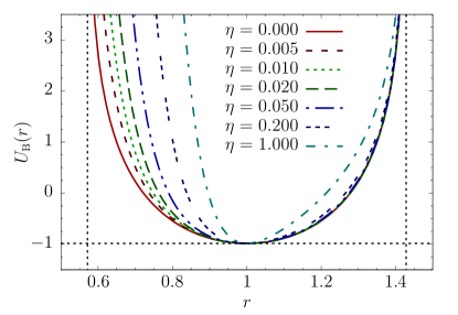
where the bond potential parameter $\eta$ controls the width and asymmetry of the potential.

The maximum bond extension is limited by the FENE potential, which diverges for $r\rightarrow r_{0}\pm R$. The FENE parameters are set to standard values $R\equiv 3/7$ and $\kappa\equiv 98/5$ Qi2014 . The Lennard-Jones potential of the bonded interaction causes an asymmetry for $\eta>0$ and reduces the potential width, while the location of the minimum $r_{0}=1$ is unchanged for this choice of parameters. The potential is shifted to have the same minimum value as in the non-bonded case: $U_{\textrm{B}}(r_{0})=-\epsilon-U_{\textrm{shift}}=U_{\textrm{NB}}(r_{0})$. Figure 1 shows the bonded potentials for various values of $\eta$. We chose $\epsilon$ as the overall energy scale and set it to unity in the simulations.

Figure 1: Potential between bonded monomers $U_{\mathrm{B}}(r)$ for different values of the parameter $\eta\in[0,1]$, which we introduced to control the range and shape of the bonded potential.

In our model, the total energy of a conformation for a polymer with $N$ monomers, $\textbf{X}=(\mathbf{r}_{1},\ldots,\mathbf{r}_{N})$, is thus given by

$$E(\textbf{X})=\sum\limits_{j=1}^{N-2}\sum\limits_{k=j+2}^{N}U_{\textrm{NB}}(r_{jk})+\sum\limits_{j=1}^{N-1}U_{\textrm{B}}(r_{j\,j+1}),$$ (4)

where $r_{jk}=|\mathbf{r}_{j}-\mathbf{r}_{k}|$ is the distance between monomers $j$ and $k$.

II.2 Simulation Method

We performed parallel tempering simulations SwendsenWangPT ; GeyerPT ; HukushimaNemotoPT ; HansmannPT for $21$ different values of $\eta\in[0,1]$ to measure thermodynamic and structural quantities needed for the structural analysis. In our implementation of this replica-exchange Monte Carlo method, Metropolis sampling was performed at temperatures $T_{i}\in[0.11,3.00]$ with $i=1,2,\ldots,I$. The number of temperature threads $I$ ranged from 96 to 128, depending on the level of complexity imposed on the system by the different choices of the model parameter $\eta$. At each temperature, random displacement updates $\mathbf{r}\rightarrow\mathbf{r}+\mathbf{d}$ were performed within a cubic box with edge lengths $l_{i}>|d_{n}|,n=1,2,3$. The size of the box $l_{i}$ was adjusted for every temperature thread separately prior to the simulation in order to achieve a Metropolis acceptance rate of approximately $50\%$. To facilitate the decorrelation of structures, exchanges of replicas between neighboring temperatures were proposed and accepted with the exchange probability

$$P(E_{i},\beta_{i};E_{i+1},\beta_{i+1})=\min\left(1,e^{(E_{i}-E_{i+1})(\beta_{i}-\beta_{i+1})}\right),$$ (5)

where $\beta=1/k_{\mathrm{B}}T$ (with $k_{\mathrm{B}}\equiv 1$ in the simulations). The temperatures $T_{i}$ were chosen equally distant in $\beta$ space to guarantee sufficiently high exchange probabilities in the low-temperature regime, where large autocorrelation times are expected Qi2014 . Between each of the $10^{6}$ replica exchanges, $10^{3}$ Metropolis Monte Carlo sweeps were performed.

For each ensemble generated in the parallel-tempering simulation, an estimate of the density of states $\overline{g}_{i}(E)$ was calculated from the energy histogram of the single-temperature canonical ensemble $h_{i}(E)$, utilizing $\overline{g}_{i}(E)=h_{i}(E)e^{\beta E}$. The estimated density of states calculated for a particular value of $\beta_{i}$ is a relative quantity which is only reliable in the energy region that is adequately covered by the ensemble of states statistically representative at this temperature. We used the multi-histogram reweighting method Swendsen1989 ; Rosenberg1992 to combine the estimates of the density of states obtained from the different temperature threads. The estimator $\hat{g}(E)$ for the density of states covering the whole energy space sampled is thus given by

$$\hat{g}(E)=\frac{\sum_{i=1}^{I}h_{i}(E)}{\sum_{i=1}^{I}M_{i}\hat{Z}_{i}^{-1}e^{-\beta_{i}E}},$$ (6)

where $M_{i}$ is the total number of sweeps and $\hat{Z}_{i}$ the individual partition function estimator in the $i$-th thread,

$$\hat{Z}_{i}=\sum_{E}\hat{g}(E)e^{-\beta_{i}E}.$$ (7)

This system of equations is iterated until convergence is achieved.

We also performed parallel simulations of multicanonical sampling Berg1991 ; Berg1992 ; Janke1998 ; Berg2000 ; Berg2003 ; Zierenberg2013 ; Michael2014Book as a supportive method for the structural analysis of the solid phase. Multicanonical sampling is more effective at overcoming hidden free-energy barriers associated with first-order transitions than parallel tempering schemes which do not artificially enhance the sampling of entropically suppressed regions in phase space. This combination of simulation methods enabled the verification of the simulation results achieved by parallel tempering and the estimates for the density of states to be used in the microcanonical statistical analysis.

II.3 Generalized Microcanonical Inflection-Point Analysis Method

For the identification and classification of the structural polymer phases, we use the recently developed generalized microcanonical inflection-point method qb1 . This statistical analysis method consequently combines microcanonical thermodynamics Gross2001 and the principle of minimal sensitivity Stevenson1981 ; Stevenson1981b , and generalizes earlier approaches Schnabel2011 limited to low-order transitions. As it turns out, though, higher-order phase transitions are potentially relevant as well, but have widely been ignored in conventional canonical analyses. Typical first- and second-order indicator functions (order parameters and response functions) are not sensitive enough to expose higher-order transition signals.

The general idea is to focus on the essential quantities entropy and energy, which govern any possible macroscopic behavior of a physical system in response to environmental conditions. In other words, the response is already encoded in the system’s energetic and entropic properties. Consequently, entropy can be defined microcanonically as the logarithm of the available energetic phase space. This makes entropy dependent of energy and the sole function that governs the system behavior. It is common to introduce the microcanonical entropy, up to an irrelevant constant, by the logarithm of the density of states,

$$S(E)=k_{\mathrm{B}}\ln\,g(E),$$ (8)

where $k_{\mathrm{B}}$ is the Boltzmann constant. Alternatively, the integrated density of states $\int_{E_{0}}^{E}dE^{\prime}\,g(E^{\prime})$ (integrating from the ground-state energy $E_{0}$) can be used as well as a representative of the energetic phase-space volume, but both versions lead to virtually identical results near the most interesting features, phase transitions, as entropy varies rapidly in these energy regions. We use the simpler form (8) in the following.

The microcanonical entropy and its derivatives have a well-defined monotonic behavior within energy regions associated with a single phase. A transition between significantly different macrostates, however, disturbs the monotony and is signaled by inflection points. Referring to the principle of minimal sensitivity, only least-sensitive inflection points have a physical meaning, though. Including the derivatives of $S(E)$ in this consideration enables the introduction of a systematic identification and classification scheme for phase transitions qb1 , reminiscent of Ehrenfest’s idea of using thermodynamic potentials ehrenfest1 . However, microcanonical inflection-point analysis is not based on the response of the system to changes of external thermodynamic state variables such as the (canonical) temperature.

If $S(E)$ contains a least-sensitive inflection point, it must clearly be signaled by a minimum in the first derivative, which is the microcanonical temperature

$$\beta(E)=T^{-1}(E)=dS(E)/dE.$$ (9)

We classify this as a first-order transition signal. In consequent analogy, we define second-order transitions by means of least-sensitive inflection points in $\beta(E)$. If a least-sensitive inflection point occurs first in the second derivative, which is symbolized by $\gamma(E)=d^{2}S(E)/dE^{2}$, we refer to it as a third-order transition, etc.

Generally, transitions of odd order $(2\nu-1)$ ($\nu$ positive integer) possess a least-sensitive inflection point in the $(2\nu-2)$th derivative of $S(E)$, which is characterized by a positive-valued minimum in

$$\left.\frac{d^{(2\nu-1)}S(E)}{dE^{(2\nu-1)}}\right|_{E=E_{\mathrm{tr}}}>0.$$ (10)

Transitions of even order $2\nu$ are least sensitive at the transition energy in the $(2\nu-1)$th derivative of $S(E)$ and the corresponding maximum in the $(2\nu)$th derivative must be negative:

$$\left.\frac{d^{2\nu}S(E)}{dE^{2\nu}}\right|_{E=E_{\mathrm{tr}}}<0.$$ (11)

We call this class of transitions independent, because there is another category, dependent transitions, which can only occur as precursors of independent transitions qb1 . In this paper, we can focus on independent transitions as dependent transitions were not observed for this model.

Note that due to binning, i.e., the discretization of the energy space in the simulations, the numerical results for the entropy are discrete. Employing discrete differentiation methods naively to get the derivatives needed for the subsequent microcanonical analysis would enhance the noise associated with the numerical error of the data and obscure transition signals. Therefore, we use the discrete set of $Q+1$ data points $S_{q}$ at energies $E_{q}$ (with $q=0,1,\ldots,Q$) obtained in the simulations as control points for the Bézier algorithm Bezier1968 ; Gordon1974 ; Michael2014Book , which generates the smooth function

$$S_{\mathrm{bez}}(E)=\sum_{q=0}^{Q}\binom{Q}{q}\!\left(\frac{E_{Q}-E}{E_{Q}-E_{0}}\right)^{Q-q}\!\left(\frac{E-E_{0}}{E_{Q}-E_{0}}\right)^{q}S_{q}.$$ (12)

The derivatives required for the statistical analysis can be calculated from this function.

Although we do not expect to observe divergences in the transition region for finite systems, we do find clear signals indicating structural transitions in the microcanonical curves, which serve as finite-system analogs of classical phase transitions. The order of these structural transitions is discernible from subtle details of the relationship between microcanonical entropy or its derivatives and the energy of the system. This approach is not based on catastrophic behavior of thermodynamic quantities. Consequently, it does not require a scaling analysis in the artificial thermodynamic limit of infinitely large systems, which for many realistic systems (such as biopolymers) is not even possible.

III Results

III.1 Canonical Statistical Analysis

Canonical analysis is the conventional approach to understanding thermodynamic properties of a system. Extremal thermal fluctuations of any observable $O$, defined by

$$\frac{d}{dT}\langle O\rangle=\frac{\langle OE\rangle-\langle O\rangle\langle E\rangle}{k_{\rm B}T^{2}},$$ (13)

are used to locate regions of temperature space with enhanced thermal activity. The most commonly considered observable is the system energy $E$, which is readily available from the simulations since Monte Carlo simulations require its calculation after each update. The thermal fluctuation of the energy, the heat capacity $C_{V}(T)=d\langle E\rangle/dT$, is a useful generic indicator for transitions in complex systems. Peaks in the $C_{V}(T)$ curve signal rapid changes of $\langle E\rangle(T)$, which typically accompany significant macrostate changes of the system like in thermodynamic phase transitions. More specific for locating structural transitions in polymer systems, we also estimated the squared radius of gyration,

$$R^{2}_{\mathrm{gyr}}=\frac{1}{N}\sum_{j=1}^{N}\left(\mathbf{r}_{j}-\mathbf{r}_{\mathrm{c.m.}}\right)^{2},$$ (14)

where $\mathbf{r}_{j}$ is the coordinate of monomer $j$ and $\mathbf{r}_{\mathrm{c.m.}}=\sum_{j=1}^{N}\mathbf{r}_{j}/N$ is the center of mass of the polymer conformation. The radius of gyration can be interpreted as a measure for structural compactness and, therefore, helps to distinguish structural phases in which the macrostates notably differ in size. The corresponding thermal fluctuation quantity $d\langle R_{\mathrm{gyr}}^{2}\rangle/dT$ is particularly useful for the identification of structural transitions if $C_{V}$ fails to provide a pronounced signal. This typically occurs for entropy-driven transitions in small systems that do not exhibit large energetic fluctuations. The most prominent example is the coil-globule (or $\Theta$) transition in finite polymer systems.

Figure 2 shows the plots of $d\langle R_{\mathrm{gyr}}^{2}\rangle/dT$ and $C_{V}$ of the 55-mer as functions of temperature $T$ for various $\eta$ values, respectively. The clearly visible peaks in the fluctuations of structural compactness at $T\approx 1.6$ in Fig. 2(a) indicate the $\Theta$ transition, where extended coil structures collapse and form the more compact globules. Increasing $\eta$ slightly shifts the $\Theta$ transition point to lower temperatures.

Figure 2: (a) and (b) Thermal fluctuation of the squared radius of gyration $d\langle R_{\mathrm{gyr}}^{2}\rangle/dT$ as a function of temperature for a flexible polymer with $N=55$ monomers at different values of $\eta$, (c) low-temperature region of the heat capacity $C_{V}$.

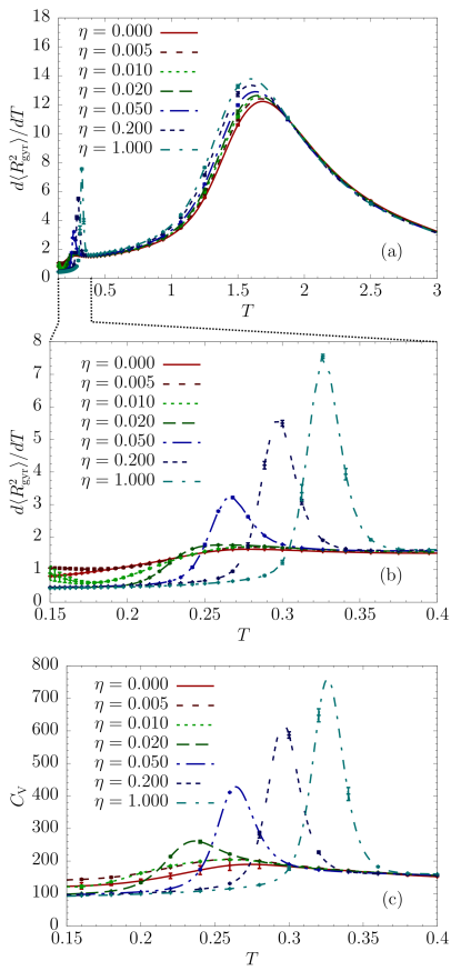
By lowering the temperature further, globular structures eventually freeze into solid conformations. The corresponding transition signals can be observed in the group of peaks at temperatures around $T=0.3$ [Figs. 2(b, c)]. These transition signals shift to lower temperatures for small $\eta$ values but start to move up in temperature for $\eta\geq 0.2$. This observation suggests a significant change in system behavior if $\eta$ exceeds a certain threshold value. Among these visible features, the signals with narrow widths and high peak heights at $\eta\geq 0.2$ indicate the freezing transition. These signals become less pronounced and broader as $\eta$ decreases. Instead of being indicators for a specific type of transition, these wide and low peaks are rather envelopes of multiple transition signals. This ambiguity in distinguishing and classifying the transitions at small $\eta$ values is caused by finite-size effects which cannot be resolved by means of canonical statistical analysis of $C_{V}$ and $d\langle R_{\mathrm{gyr}}^{2}\rangle/dT$. Therefore, it is necessary to employ other systematic and robust methods such as microcanonical inflection-point analysis, which can clearly distinguish the sensitive transition signals in finite-size systems. Subsequent structural analysis will then enable us to interpret the physical meaning of these transition signals.

III.2 Microcanonical Analysis and
Hyperphase Diagram

Figure 3: (a) Microcanonical entropy $S(E)$ for an array of $\eta$ values; (b) microcanonical inverse temperature $\beta(E)=dS/dE$; (c) $\gamma(E)=d\beta(E)/dE$; (d) $\delta(E)=d\gamma(E)/dE$.

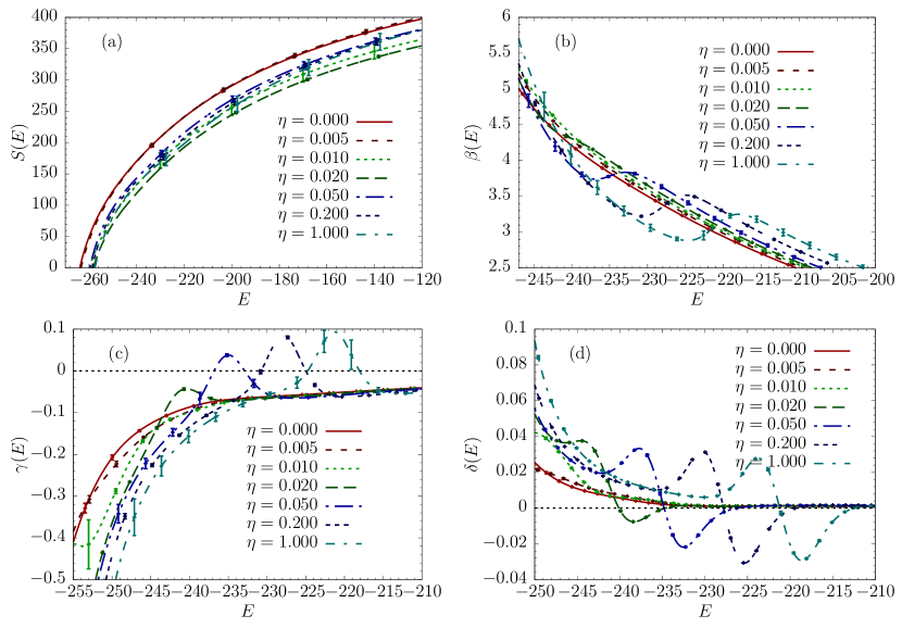
As discussed earlier, microcanonical inflection-point analysis Schnabel2011 ; Michael2014Book ; qb1 can be used to identify and classify transitions in systems of any size. In the following, we focus on the transition behavior of polymer models with $\eta\in[0,1]$ at low temperatures. Plots of the microcanonical entropy $S(E)$ are shown in Fig. 3(a). Simulations for $\eta\geq 0.04$ reveal least-sensitive inflection points and a convex region in the entropy curves, leading to the prominent “backbending behavior” in the $\beta(E)$ plots shown in Fig. 3(b). According to the generalized inflection-point analysis method qb1 , minima of $\beta(E)$ are indicative of a first-order transition. At $\eta=0.04$, the first-order transition is found at $T\approx 0.25$. It is stable for $\eta\geq 0.04$ and the transition temperature increases slightly with $\eta$. This is the expected first-order transition from the liquid to a solid phase, which is known to be the icosahedral phase for the 55-mer studied here. These results enable us to construct the low-temperature transition line in the hyperphase diagram shown in Fig. 4(a).

Below $\eta\approx 0.04$, the scenario is significantly different. The negative-valued peak for $\eta=0.02$ at $E\approx-241$ corresponds to a least-sensitive inflection point in $\beta(E)$, which indicates a second-order transition at $T\approx 0.23$. Systematic analysis reveals that this transition type occurs in the interval $0.01<\eta<0.04$ and replaces the first-order liquid-solid transition in this temperature region. As the structural analysis in the following section will show, the liquid-solid transition behavior becomes indeed more complex. This is also due to the occurrence of additional transition signals of higher order. At $\eta\approx 0.012$ we find a third-order transition signal in this transition region, which marks the crossover point towards a fourth-order transition for $\eta<0.01$.

Another remarkable feature of the small-$\eta$ models is the occurrence of additional precursor lines that “shadow” the major low-$T$ transition line. Their existence is unmistakably manifest from the positive-valued minima in the $\delta(E)$ curves shown in Fig. 3(d), which indicate third-order transitions. For $\eta>0.025$, these transition points lie below the liquid-solid transition line, for $\eta<0.025$ above the extension of this line. This qualitative change is another indication that the structural behavior of the system significantly changes around this crossover point. It is worth noting that the shadow transition keeps accompanying the liquid-solid line even for larger $\eta$ values. It approaches the strong first-order line asymptotically and merges with it (in microcanonical analysis, a transition line is swallowed by a first-order transition, if the former enters the backbending region of the latter).

Figure 4: (a) Microcanonical hyper-phase diagram, parameterized by temperature $T$ and model parameter $\eta$. The major phases are labeled G (gas), L (liquid), and S (solid). (b) Detail view of the low-temperature and small-$\eta$ region, emphasizing the different solid phases. In S_bi-core, structures with bihexagonal cores and liquid-like shells are dominant. S_ic-core represents conformations with well-formed icosahedral cores, but incomplete surface layer. In the S_ic and S_bi pseudophases, icosahedral and bihexagonal core structures have complete overlayers. In S_mix icosahedral and bihexagonal core structures coexist. The “solid” subphases are separated by gray empirical transition bands. Dashed lines represent lines of transitions higher than second order.

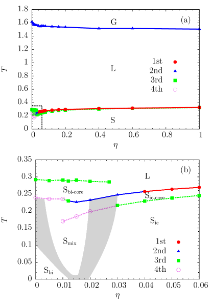
Based on the results obtained by microcanonical inflection-point analysis for 19 $\eta$ values, we construct the hyperphase diagram as shown in Fig. 4(a). The major phases are well-known from previous studies of flexible polymers. At sufficiently high temperatures, the polymer is in the gas-like pseudophase in which dissolved or random-coil structures dominate. Decreasing the temperature causes the polymer to collapse and to enter the liquid pseudophase, where compact globular conformations are favorably formed. The corresponding pseudophase transition is the well-known $\Theta$-transition (collapse transition). Because of the negative $\gamma(E)$ peaks for all $\eta$ values in this region, this transition is classified as of second order and it is represented by the blue line in Fig. 4(a). As the temperature decreases further, the polymer transfers from the globular phase to the more compact “solid” phase (liquid-solid or freezing transition), which is characterized by locally crystalline or amorphous metastable structures.

The analysis of the compact subphases is much more challenging as the magnification of the low-temperature and small-$\eta$ region of the hyper-phase diagram in Fig. 4(b) shows. Multiple transition lines of different order exist. Microcanonical inflection-point analysis identifies the liquid-solid transition as of first order for $\eta>0.04$ and of second order for $0.01<\eta<0.04$. The extension of this line for $\eta<0.01$ is of higher than second order. The detailed structural analysis in the next section will shed more light on the reasons for this diverse and complex behavior, which includes additional transition lines. Most notably, the liquid-solid transition is accompanied by a third-order transition line. Both lines eventually merge for large $\eta$ values. Structures in the intermediate phase possess a solid icosahedral core, whereas the overlayers are still disorganized and incomplete, forming a two-dimensional liquid interface. Only for temperatures below this companion line and sufficiently large $\eta$ values, the phase is dominated by structures with icosahedral geometry as it is expected for a flexible polymer with a “magic” number of monomers and matching length scales of bonded and nonbonded interactions.

For $\eta<0.03$, different geometric subphases exist and are characterized by the competition between structures with icosahedral and bihexagonal cores (see Fig. 5). Only for smallest $\eta$ values and lowest temperatures, the bihexagonal phase dominates. This is an interesting result as it shows that the solid phase of polymers with symmetric and wider bond potentials is indeed different, but stable only for small variations of parameters. If the threshold value $\eta\approx 0.02$ is exceeded, though, icosahedral structures mix in and eventually dominate for larger parameter values.

III.3 Structural analysis

The tools of microcanonical inflection-point analysis, as introduced in the previous section, provide us with a systematic way of identifying and classifying all structural transitions in a given physical system. Another step towards a more advanced understanding of thermodynamic properties of a system is the identification of dominant conformations and their abundance in a relevant energy range. This can be done directly either by visual inspection of sample structures, or more systematically, by introducing a suitable set of structural order parameters.

Figure 5: Core structures in solid phases of the 55-mer: (a) icosahedral (ic-core); (b) bihexagonal (bi-core).

Figure 6: Intensity plots of the $Q_{6}$ order parameter at (a) $\eta=0.005$, (b) $\eta=0.010$, (c) $\eta=0.020$, and (d) $\eta=0.050$, respectively. The probability of finding polymer structures with a particular value of $Q_{6}$ is represented by colored shading, with black being zero probability and red corresponding to the maximum probability of $1$.

For the purpose of identification of low-energy solid-like structures which possess well-defined symmetries, a set of effective order parameters can be defined in terms of the real spherical harmonics kqb1 . We define the polymer core as consisting of $K$ monomers with the coordinates $\mathbf{X}^{\mathrm{C}}=(\mathbf{r}^{\mathrm{C}}_{1},\ldots,\mathbf{r}^{\mathrm{C}}_{K})$ within 1.25$\sigma$ of the center of mass of the polymer. We introduce a set of rotationally invariant order parameters by

$$Q_{l}=\left[\frac{4\pi}{2l+1}\sum_{m=-l}^{l}|\rho_{lm}|^{2}\right]^{1/2},$$ (15)

where

$$\rho_{lm}=\frac{1}{K}\sum\limits_{k=1}^{K}Y_{lm}(\mathbf{r}^{\mathrm{C}}_{k})$$ (16)

is the average of the real spherical harmonics

$$Y_{lm}(\mathbf{r})=\begin{cases}\vspace{1mm}\frac{i}{\sqrt{2}}\left[Y_{l}^{m}(\mathbf{r})-(-1)^{m}Y_{l}^{-m}(\mathbf{r})\right],&m<0,\\[2.84526pt] Y_{l}^{m}(\mathbf{r}),&m=0,\\[2.84526pt] \frac{1}{\sqrt{2}}\left[Y_{l}^{-m}(\mathbf{r})+(-1)^{m}Y_{l}^{m}(\mathbf{r})\right],&m>0\end{cases}$$ (17)

calculated at the positions of the core monomers.

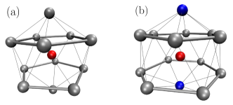
As expected, preliminary inspection of structures obtained from simulations of the flexible 55-mer with $\eta\approx 1$ shows that below the freezing transition virtually all conformations contain an icosahedral core. However, with virtually symmetric bonded interactions $(\eta<0.03)$, two distinct core geometries are found. In addition to the standard icosahedral core, which is present in the global minimum structures of most short chains, we have also identified a bihexagonal core consisting of 15 monomers (Fig. 5). The six-fold dihedral symmetry of the bihexagon and the icosahedral symmetry are best distinguished using the $Q_{6}$ order parameter. For a perfect icosahedral core, $Q_{6}\approx 0.65$, whereas a bihexagonal core corresponds to $Q_{6}\approx 0.41$.

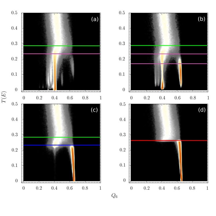
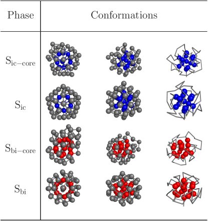
We present the results in the form of intensity plots in Fig. 6. Shades correspond to the probability of finding a structure with a particular value of $Q_{6}$ at a given microcanonical temperature $T(E)$. Black represents zero probability and red unity. An interesting feature, found only in systems with $\eta<0.027$, is marked by the green horizontal lines at $T\approx 0.29$. It is associated with the apparent shift of the peak of the $Q_{6}$ distribution at this temperature towards lower values. This indicates the onset of the formation of bihexagonal cores in the liquid phase and corresponds to the third-order transition line in the microcanonical phase diagram [Fig. 4(b)]. Below this transition, amorphous structures with loose bihexagonal cores and liquid-like surfaces are identified in the S_bi-core pseudophase. Typical conformations containing icosahedral or bi-hexagonal cores are shown in Fig. 7.

Figure 7: Different views of typical structures in the solid subphases: view along the core axis (left), perspective view (center), and core representation (right). Icosahedral and bihexagonal cores are plotted in blue and red, respectively. Gray beads represent surface monomers.

At low temperatures and $\eta=0.005$, we observe a single dominant funnel centered at $Q_{6}\approx 0.41$, containing structures with a bihexagonal core [Fig. 6(a)]. The adjacent secondary funnels all contain bihexagonal cores with slightly modified inter-monomer distances. Structures with an icosahedral core are found in the weakly populated funnel at $Q_{6}\approx 0.65$. The low-temperature transition signal is associated with the increase in the population of structures with bihexagonal cores and is classified as of fourth order. This transition signal is marked by violet transition lines in Fig. 6(a) and in the hyper-phase diagram shown in Fig. 4(b). A small increase in the strength of the bonded LJ potential leads to a sharp increase in the population of icosahedral cores. For $\eta=0.01$, the ground state of the polymer is still found in the bihexagonal funnel, however the onset of a significant population of icosahedral cores produces an additional fourth-order transition signal at $T=0.17$, see Fig. 4(b) and Fig. 6(b). Further increase leads to a sharp decline in the population of the bihexagonal funnel.

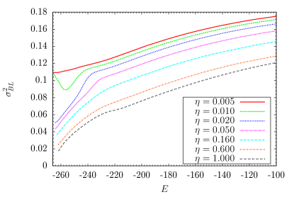
This can be seen clearly for $\eta\geq 0.02$ [Fig. 6(c), (d)] where the energetic penalty for non-optimal bond lengths becomes too large to accommodate structures with bihexagonal cores. Indeed, their formation requires significant variance in bond lengths, whereas icosahedral cores can be formed with near-optimal values. For $\eta\approx 0$, the pure FENE potential permits large bond fluctuations. However, with the introduction of the bonded LJ potential these fluctuations cause an energetic penalty. This explains why the bihexagonal funnel exists only if the bonded LJ potential is sufficiently weak. In Fig. 8, we show the bond-length variance as a function of energy for different values of the model parameter $\eta$. With increasing values of $\eta$ the variance decreases, most significantly in the low-energy region. Most striking is the difference between the low-energy curves for $\eta=0.01$ and $\eta=0.02$, where the former has a bihexagonal ground-state and the latter is icosahedral.

Figure 8: Variance $\sigma^{2}_{\mathrm{BL}}$ of bond-length fluctuations for the 55-mer plotted as a function of energy and different values of the model parameter $\eta$.

At $\eta\approx 0.04$, the signal associated with the onset of the icosahedral funnel becomes first order and can be unambiguously identified as the freezing transition. Beyond $\eta\approx 0.1$, the structural and energetic properties of the 55-mer do not change significantly anymore.

From the structural analysis, we conclude that the low-temperature behavior of this flexible polymer model can be classified into three pseudophases. For sufficiently small $\eta$ values, bihexagonal core structures with compact hexagonal-like surface layers, shown in Fig. 7, dominate the solid phase. As $\eta$ is increased, the population of icosahedral structures gradually increases due to the additional energy penalty of the non-optimal bond lengths in bihexagonal cores, but both structure types still coexist in a mixed phase [$S_{\mathrm{mix}}$ in the Fig. 4(b)]. Once the width of the bonded potential is sufficiently narrow, the bihexagonal core structures completely vanish and only the icosahedral structures persist. The corresponding pseudophase is labeled $S_{\mathrm{ic}}$ in Fig. 4 and representative structures are shown in Fig. 7.

The third-order transition accompanying the freezing transition in Fig. 4(b) is associated with the completion of the icosahedral shell. Upon decreasing the temperature, liquid structures begin to nucleate and first form the stable icosahedral cores if $\eta>0.03$. Surfaces of the polymer structures still undergo large fluctuations in order to arrange the surface monomers in optimal locations. The mobility of the monomers is confined to effectively two dimensions on the surface. These semi-liquid structures are dominant in the solid $S_{\mathrm{ic-core}}$ pseudophase. If the temperature is decreased further, the surface formation finishes and complete icosahedral shell structures appear in the solid $S_{\mathrm{ic}}$ pseudophase.

For sufficiently large $\eta$ values, the freezing transition of a polymer can generally be characterized by two hierarchical processes. One is associated with the nucleation process of the core identified as first- or second-order transitions and the other is due to surface layer formation which is a third-order transition.

IV Concluding Remarks

We employed parallel tempering simulations, supported by a parallelized version of multicanonical sampling, to investigate the effects of the shape of the potential of bonded monomers on the structure formation properties of elastic flexible polymers. For this purpose, we introduced the model parameter $\eta$, which controls the width and asymmetry of the bond potential. In this study we focused on a single flexible polymer with 55 monomers, which is an interesting example as it can form a perfectly icosahedral structure under certain conditions. In order to identify and distinguish the various structural phases in this system, we systematically applied the microcanonical inflection-point analysis method and performed a thorough structural analysis of the compact phases to construct the hyperphase diagram.

Besides the commonly expected random-coil (gas-like) and globular (liquid-like) phases, we find a diversity of solid subphases whose properties depend on the value of the $\eta$ model parameter.

Perturbing the symmetric FENE potential allows for larger fluctuations of bond lengths. Structures with bihexagonal cores commonly dominate the solid phase as long as the bond potential is virtually symmetric. Increasing the value of the model parameter $\eta$ narrows the bond potential width and induces asymmetry. The energetic penalty for non-optimal bond lengths becomes too large to accommodate structures with bihexagonal cores. Thus, bihexagonal core structures become less favorable for large $\eta$ values and icosahedral cores begin to dominate, leading to a mixed phase, in which both structure types coexist. The mixed phase eventually turns into the icosahedral phase if $\eta$ is sufficiently large and the bond potential is dominated by the Lennard-Jones potential.

Our results also indicate that for sufficiently large $\eta$ values, the freezing transition is a well-organized hierarchical process: Whereas nucleation or core formation is a first-order transition, the subsequent shell formation process was identified as a separate third-order transition. During core formation, the surface layer remains liquid. This flexibility enables an optimal arrangement of the core monomers. Once the solid core is formed, the monomers of the surface layer pack optimally in the void spaces left on the surface of the core, thereby forming the second shell of the icosahedral conformation.

The results we obtained also demonstrate the power of microcanonical inflection-point analysis, which does not only help identify the major transitions but can also distinguish the details of the transition processes by signaling higher-order transitions.

Our case study of a 55-mer provides robust insights into the nature of transition processes in flexible polymers. The general structure of the hyperphase diagram discussed in this paper is not expected to change significantly for larger systems. However, it is well known that details of the liquid-solid and solid-solid transitions, typically associated with Mackay and anti-Mackay overlayer formation sbj1 , depend on the system size. Therefore, future work on the deeper analysis of these processes for other chain lengths, using the model and methodologies introduced in this paper, would be intriguing.