Using tours to visually investigate properties of new projection pursuit indexes with application to problems in physics
Abstract
Projection pursuit is used to find interesting low-dimensional
projections of high-dimensional data by optimizing an index over all
possible projections. Most indexes have been developed to detect
departure from known distributions, such as normality, or to find
separations between known groups. Here, we are interested in finding
projections revealing potentially complex bivariate patterns, using new
indexes constructed from scagnostics and a maximum information
coefficient, with a purpose to detect unusual relationships between
model parameters describing physics phenomena. The performance of these
indexes is examined with respect to ideal behaviour, using simulated
data, and then applied to problems from gravitational wave astronomy.
The implementation builds upon the projection pursuit tools available in
the R package, tourr, with indexes constructed from code in the R
packages, binostics, minerva and mbgraphic.
1 Introduction
The term “projection pursuit” (PP) was coined by Friedman and Tukey (1974) to describe a procedure for searching high (say )dimensional data for “interesting” low-dimensional projections ( or usually). The procedure, originally suggested by Kruskal (1969), involves defining a criterion function, or index, that measures the “interestingness” of each -dimensional projection of -dimensional data. This criterion function is optimized over the space of all -dimensional projections of -space, searching for both global and local maxima. It is hoped that the resulting solutions reveal low-dimensional structure in the data not found by methods such as principal component analysis. Projection pursuit is primarily used for visualization, with the projected data always reported as plots.
A large number of projection pursuit indexes have been developed, primarily based on departure from normality, which includes clusters, outliers and skewness, and also for finding separations between known groups (e.g. Friedman (1987), Hall (1989) Cook, Buja, and Cabrera (1992), Naito (1997), Lee et al. (2005), Ahn, Hofmann, and Cook (2003), Hou and Wentzell (2014), Jones and Sibson (1987), Rodriguez-Martinez et al. (2010), Pan, Fung, and Fang (2000), Ferraty et al. (2013), Loperfido (2018)). Less work has been done on indexes to find nonlinear dependence between variables, focused on , which motivates this research.
The driving application is from physics, to aid the interpretation of model fits on experimental results. A physical model can be considered to be a set of free parameters, that cannot be measured directly and are determined by fitting a set of experimental observations, for which predictions can be made once the parameters are estimated. (Note here, that while we may have analytic expressions for the predictions, this is not always the case and we often have to rely on numerical computation.) Different sets of model parameters () found to be compatible with the experimental results within a selected level of confidence yield the data to be examined using projection pursuit. A single prediction can be a complicated function of all of the free parameters, and typically and . Current practice is to examine pairs of parameters, or combinations produced by intuition or prior knowledge. This begs the question, whether important nonlinear associations are missed because they are hidden in linear combinations of more than two variables.
PP can be combined with other dimension reduction methods when is very high. For example, it can be beneficial to first do principal component analysis prior to PP, especially to remove linear dependencies before searching for other types of association. This is the approach used in Cook, Laa, and Valencia (2018), which explores a 56-dimensional parameter space, by first reducing the number of dimensions to the first six principal components, before applying projection pursuit. PCA was appropriate for this problem because reducing to principal component space removed the linear dependencies while preserving the nonlinear relationships that were interesting to discover. Some projection pursuit indexes do incorporate penalty terms to automate removing noise dimensions. It can also be important to have an efficient PP optimizer, particularly when working with high dimensions, because the search space increases exponentially with dimension.
To find appropriate projections pursuit indexes for detecting nonlinear dependencies, the literature on variable selection was a starting point. With high-dimensional data, even plotting all pairs of variables can lead to too many plots, which is what “scagnostics” (Wilkinson, Anand, and Grossman (2005), Wilkinson and Wills (2008)) were developed to address by providing metrics from which to select the most interesting variable pairs. There are eight scagnostics, of which three (“convex”, “skinny” and “stringy”) are used here. The question is whether these can be adapted into projection pursuit indexes, to search for unusual features in two-dimensional projections of high-dimensional data. Recent PhD research by Grimm (2016) explored the behavior of scagnostics for selecting variables, and proposed two more that have nicer properties, based on smoothing splines and distance correlation. In addition, two more indexes for measuring dependence have been proposed in the machine learning literature, based on information criteria, maximal and total information coefficient (MIC and TIC) (Reshef et al. 2011), with computationally more efficient versions (MIC_e, TIC_e) (Reshef et al. 2016). These are related to original 1D projection pursuit indexes based on entropy (e.g. Huber (1985), Jones and Sibson (1987)). This provides seven current indexes for measuring dependence between two variables, and each is available in an R (R Core Team 2018) package: binostics (Hofmann et al. 2019), mbgraphic (Grimm 2017) and minerva (Albanese et al. 2012).
PP index behavior can be understood and investigated more substantially when combined with a tour. A tour (Asimov (1985), Buja et al. (2005)) displays a smooth sequence of low dimensional projections from high dimensions to explore multivariate data for structure such as clusters, outliers, and nonlinear relationships. Cook et al. (1995) provided an approach combining the tour algorithm with PP, to interactively both search for interesting projections, and examine the behavior of the indexes. The projection pursuit guided tour is available in the R package, tourr (Wickham et al. 2011), and provides optimization routines, and visualization.
This paper is structured as follows. Section 2 discusses index construction, and how they can be used in the guided tour. Section 3 investigates the behavior of the indexes, explored primarily using tour methods. The new guided tour with these indexes is applied to two examples from gravitational wave astronomy (Section 4). The latter two parts are connected in that the application of the new indexes to these problems is the main motivation for the paper, and the simulation study, in the first part, was conducted to better understand the behavior of the indexes in general. The techniques in Section 3 define procedures that will be generally useful for researchers developing new projection pursuit indexes to visually assess their behavior. Visual methods to diagnose the index behavior is important because PP is primarily used for visualization. The paper finishes with a discussion about the limitations of this work, and the potential future directions.
2 Projection pursuit index construction and optimization
A projection pursuit index (PPI) is a scalar function defined on an -dimensional data set, computed by taking a -dimensional projection of an data matrix. Typically the definition is such that larger values of indicate a more interesting distribution of observations, and therefore maximizing over all possible dimensional projections of a data set with variables will find the most interesting projections. This section describes the seven indexes that are to be used to explore bivariate association. Some data pre-processing, including standardization, is advisable, prior to optimizing the PPI.
2.1 Scaling and standardization
Making a plot always involves some choice of scaling. When a scatterplot is made, effectively, albeit under the hood, the data is scaled into a range of (often ) on both axes to print it on a page or display in a graphics device window. The range deliminates page space within which to draw. The upshot is that the original data scale is standardized to the range and aspect ratio on the display space. It may be that the original range of one variable is and the other is but the display linearly warps this to and , say, giving both variables equal visual weight.
With high dimensional data, and particularly projections, it is also necessary to re-scale the original range, and it is important to pay attention to what is conventional, or possible, and the effects. The PPIs also may require specific scaling for them to be effectively computed. Both of these are addressed here. The common pre-processing include:
-
•
Standardizing each variable, to have mean 0 and variance 1, so that individual variable scales do not affect the result. Different variable scales are examinable without resorting to projection pursuit, so can be handled prior to searching through high dimensions.
-
•
Sphering the high-dimensional data is often done to remove linear dependence. This is typically done using principal component analysis, and using the principal components as the variables passed to PP. If linear dependence is the only structure PP is not needed, and thus this is removed before PP so that the PPIs are not distracted by simple structure.
-
•
Transform single variables to reduce skewness. It is marginal structure, visible in a single variable, which doesn’t need a multivariate technique to reveal. Skewed distributions will inadvertently affect the PPIs, distracting the search for dependence.
-
•
Remove outliers, which may be an iterative process, to discover, identify and delete. Extreme values will likely affect PPI performance. Outliers can be examined on a case by case basis later.
-
•
Possibly remove noise dimensions, which is also likely to be an iterative process. Directions where the distribution is purely noise make optimization of a PPI more difficult. If a variable is suspected to have little structure and relationship with other variables, conducting PP on the subset of variables without them may improve the efficiency of the search.
-
•
Centering and scaling of the projected data, can be helpful visually. If the data has a small amount of non-normal distribution in some directions, the projected data can appear to wander around the plot window during a tour. It doesn’t matter what the center of the projected data is, so centering removes a wandering scatterplot. Less commonly, it may be useful to scale the projected data to standard values, which would be done to remove any linear dependence remaining in the data.
| be the number of variables in the data. For physics models the observable space is higher dimension, say , and the data examined is the fitted model space, typically less than 10. | |
| projection dimension. For studying physics models, typically and this is the focus for the index definition. | |
| Number of observations, which for the physics models is the number of fitted models being examined and compared. | |
| -dimensional data matrix, where variables may be scaled or standardized, and may be sphered | |
| projected data matrix. where | |
| orthonomal projection matrix | |
| Convex hull | |
| Alpha hull |
2.2 New projection pursuit index functions
Table 1 summarizes the notation used for this section. Here we give an overview of the functions that are converted into projection pursuit indexes. Full details of the functions can be found in the original sources.
-
•
scagnostics: The first step to computing the scagnostics is that the bivariate data is binned, and scaled between [0,1] for calculations. The convex (Eddy 1977) and alpha hulls (Edelsbrunner, Kirkpatrick, and Seidel 1983), and the minimal spanning tree (MST) (Kruskal 1956), are computed.
-
–
convex: The ratio of the area of alpha to convex hull, . This is the only measure where interesting projections will take low values, with a maximum of 1 if both areas are the same. Thus is used.
-
–
skinny: The ratio of the perimeter to the area of the alpha hull, , where the normalization is chosen such that for a full circle. Values close to 1 indicate a skinny polygon.
-
–
stringy: Based on the MST, where the diameter is the longest connected path, and the length is the total length (sum of all edges). If the MST contains no branches .
-
–
-
•
association: The index functions are available in Grimm (2017), and are defined to range in [0,1]. Both functions in the mbgraphic package can bin the data before computing the index, for computational performance.
-
–
dcor2D: This function is based on distance correlation (Székely, Rizzo, and Bakirov 2007), which is designed to find both linear and nonlinear dependencies between variables. It involves computing the distances between pairs of observations, conducting an analysis of variance type breakdown of the distances relative to each variable, and the result is then passed to the usual co variance and hence correlation formula. The function wdcor, in the R package, extracat (Pilhöfer and Unwin 2013), computes the statistic, and the mbgraphic package utilises this function.
-
–
splines2D: Measures nonlinear dependence by fitting a spline model (Wahba 1990) of on and also on , using the gam function in the R package, mgcv (Wood et al. 2016). The index compares the variance of the residuals:
(1) which takes large values if functional dependence is strong.
-
–
-
•
information: The index functions (Reshef et al. 2011) nonparametricly measure nonlinear association by computing the mutual information,
(2) where are binned values of the projected data, and is the relative bin count in each cell, and are the row and column relative counts, on a range of bin resolutions of the data. It is strictly a 2D measure. For a fixed binning, e.g. or , the optimal binning is found by maximizing . The values of I range between because they are normalized across bins by dividing by .
-
–
Maximum Information Coefficient (MIC): uses the maximum normalized across all bin resolutions.
-
–
Total Information Coefficient (TIC): sums the normalized for all bin resolutions computed. This creates a problem of scaling - there is no upper limit, although it is related to number of bins, and number of bin resolutions used. In the work below we have made empirical estimates of the maximum and scaled the TIC index using this to get it in the range . This index should be more stable than MIC.
-
–
A comparison between these indexes for the purpose of variable selection, but not projection pursuit, was discussed in Grimm (2016). It is only available in German, we we summarize the main findings here. The scagnostics measures are flexible, and calculating the full set of measures provides useful guidance in variable selection. However, they are found to be highly sensitive to outlying points and sample size (as a consequence of the binning). Both splines2D and dcor2D are found to be robust in this respect, but splines2D is limited to functional dependence, while dcor2D is found to take large values only in scenarios with large linear correlation. The mutual information based index functions (MIC, TIC) are found to be flexible, but are sensitive to the sample size and often take relatively large values even when no association is present. A brief comparison of MIC and dcor2D was also provided in Simon and Tibshirani (2014).
In addition to the seven indexes described above, we will also include the holes index available in the tourr package, see (Cook, Buja, and Cabrera (1993), Cook and Swayne (2007)). This serves as a benchmark, demonstrating some desired behavior. The index takes maximum values for a central hole in the distribution of the projected data.
2.3 Optimization
Given a PPI we are confronted with the task of finding the maximum over all possible dimensional projections. One challenge is to avoid getting trapped in local maxima that are only a result of sampling fluctuations or a consequence of a noisy index function. Posse (1995a) discusses the optimization, in particular that for most index functions and optimizers results are too local, largely dependent on starting point. Friedman (1987) suggested a two-step procedure: the first step is using a large step size to find the approximate global maximum while stepping over pseudomaxima. A second step is then starting from the projection corresponding to the approximate maximum and employing a gradient directed optimization for the identification of the maximum. For exploring high-dimensional data, it can be interesting to observe local maxima as well as a global maximum, and thus a hybrid algorithm that still allows lingering but not being trapped by local maxima is ideal. In addition, being able to visually monitor the optimization and see the optimal projection in the context of neighboring projections is useful. This is provided by combining projection pursuit with the grand tour (Cook et al. 1995). The properties of a suitable optimization algorithm include monotonicity of the index value, a variable step-size to avoid overshooting and to increase the chance of reaching the nearest maximum, and a stopping criterion allowing to move out of a local maximum and into a new search region (Wickham et al. 2011). A possible algorithm is inspired by simulated annealing and has been described in Lee et al. (2005), this has been implemented in the search_better and search_better_random search functions in the tourr package. The tourr package also provides the search_geodesic function, which first selects a promising direction by comparing index values between a selected number of small random steps, and then optimizes the function over the line along the geodesic in that direction considering projections up to away from the current view.
3 Investigation of indexes
A useful projection pursuit index needs to have several properties. This has been discussed in several seminal papers, e.g. Diaconis and Freedman (1984), Huber (1985), Jones and Sibson (1987), Posse (1995a), Hall (1989). The PPI should be minimized by the normal distribution, because this is not interesting from a data exploration perspective. If all projections are normally distributed, good modelling tools already exist. A PPI should be approximately affine invariant, regardless how the projection is rotated the index value should be the same, and the scale of each variable shouldn’t affect the index value. Interestingly the original index proposed by Friedman and Tukey (1974) was not rotationally invariant. A consistent index means that small perturbations to the sample do not dramatically change the index value. This is particularly important to making optimization feasible, small angles between projections correspond to small perturbations of the sample, and thus should be small changes to index value. Posse (1995a) suggests that indexes should be resistant to features in a tail of the distribution, but this is debatable because one departure from normality that is interesting to detect are anomalous observations. Some PPI are designed precisely for these reasons. Lastly, because we need to compute the PPI over many projections, it needs to be fast to compute. These form the basis of the criteria upon which the scagnostic indexes, and the several alternative indexes are examined, as explained below.
-
•
smoothness: This is the consistency property mentioned above. The index function values are examined over interpolated tour paths, that is, the value is plotted against time, where time indexes the sequence of projections produced by the tour path. The signature of a good PPI is that the plotted function is relatively smooth. The interpolation path corresponds to small angle changes between projections, so the value should be very similar.
-
•
squintability: Tukey and Tukey (1981) introduced the idea of squint angle to indicate resolution of structure in the data. Fine structure like the parallel planes in the infamous RANDU data (Marsaglia 1968) has a small squint angle because you have to be very close to the optimal projection plane to be able to see the structure. Structures with small squint angle are difficult to find, because the optimization algorithm needs to get very close to begin hill-climbing to the optimum. The analyst doesn’t have control over the data structure, but does have control over the PPI. Squintability is about the shape of the PPI over all projections. It should have smooth low values for noise projections and a clearly larger value, ideally with a big squint angle, for structured projections. The optimizer should be able to clearly see the optimal projections as different from noise. To examine squintability, the PPI values are examined on interpolated tour paths between a noise projection and a distant structured projection.
-
•
flexibility: An analyst can have a toolbox of indices that may cover the range of fine and broad structure, which underlies the scagnostics suite. Early indexes, based on density estimation could be programmed to detect fine or large structure by varying the binwidth. This is examined by using a range of structure in the simulated data examples.
-
•
rotation invariance: The orientation of structure within a projection plane should not change the index value. This is especially important when using the projection pursuit guided tour, because the tour path is defined between planes, along a geodesic path, not bases within planes. If a particular orientation is more optimal, this will get lost as the projection shown pays no attention to orientation. Buja et al. (2005) describes alternative interpolation paths based on Givens and Householder rotations which progress from basis to basis. It may be possible to ignore rotation invariance with these interpolations but there isn’t a current implementation, primarily because the within-plane spin that is generated is distracting from a visualization perspective. Rotation invariance is checked for the proposed PPIs by rotating the structured projection, within the plane.
-
•
speed: Being fast to compute allows the index to be used in real-time in a guided tour, where the optimization can be watched. When the computations are shifted off-line, to watch in replay, computation times matter less. This is checked by comparing times for benchmark scenarios with varying sample size.
3.1 Simulation study setup
3.1.1 Data construction
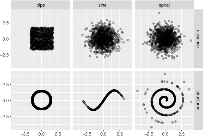
Three families of data simulations are used for examining the behavior of the index functions. Each generates structure in two variables, with the remaining variables containing various types of noise. This is a very simple construction, because there is no need for projection pursuit to find the structure, one could simply use the PPIs on pairs of variables. However, it serves the purpose to also evaluate the PPIs. The three data families are explained below. In each set, is used for the number of points, is the number of dimensions, and is the projection dimension. The three structures were selected to cover both functional and non-functional dependence, different types of nuisance distributions and different structure size and squintability properties.
-
•
pipe: nuisance directions are generated by sampling independently from a uniform distribution between , and the circle is generated by sampling randomly on a 2D circle, and adding a small radial noise. The circle should be easy to see by some indices because it is large structure, but the nonlinearity creates a complication.
-
•
sine: nuisance directions are generated by sampling independently from a standard normal distribution, and the sine curve is generated by . The sine is a medium nonlinear structure, which should be visible to multiple indices.
-
•
spiral: nuisance directions are generated by sampling independently from a normal distribution, and the structure directions are sampled from an Archimedean spiral, i.e. , with and we sample angles from a normal distribution with mean 0 and variance , giving a spiral with higher densities at lower radii. The absolute value of fixes the direction of the spiral shape. This is fine structure which is only visible close to the optimal projection.
| pipe | sine | spiral | |||||
|---|---|---|---|---|---|---|---|
| Index | lower | upper | lower | upper | lower | upper | |
| holes | noise | 0.37 | 0.46 | 0.00 | 0.01 | 0.00 | 0.01 |
| structure | 0.98 | 0.99 | 0.00 | 0.00 | 0.00 | 0.00 | |
| convex | noise | 0.70 | 0.73 | 0.57 | 0.69 | 0.54 | 0.68 |
| structure | 0.06 | 0.07 | 0.00 | 0.00 | 0.00 | 0.00 | |
| skinny | noise | 0.12 | 0.18 | 0.13 | 0.28 | 0.13 | 0.31 |
| structure | 0.84 | 0.86 | 0.76 | 0.87 | 0.84 | 0.90 | |
| stringy | noise | 0.31 | 0.48 | 0.20 | 0.42 | 0.22 | 0.43 |
| structure | 0.57 | 0.74 | 1.00 | 1.00 | 0.88 | 0.98 | |
| dcor2D | noise | 0.03 | 0.07 | 0.04 | 0.07 | 0.04 | 0.07 |
| structure | 0.17 | 0.18 | 0.96 | 0.98 | 0.14 | 0.17 | |
| splines2D | noise | 0.00 | 0.02 | 0.00 | 0.02 | 0.00 | 0.02 |
| structure | 0.00 | 0.02 | 1.00 | 1.00 | 0.01 | 0.05 | |
| MIC | noise | 0.03 | 0.04 | 0.03 | 0.04 | 0.03 | 0.05 |
| structure | 0.56 | 0.58 | 0.98 | 1.00 | 0.40 | 0.45 | |
| TIC | noise | 0.02 | 0.02 | 0.02 | 0.02 | 0.02 | 0.02 |
| structure | 0.42 | 0.43 | 0.95 | 0.98 | 0.26 | 0.30 | |
For simplicity, in the investigations of the index behavior, we fix , which corresponds to two independent 2D planes containing nuisance distributions, and one 2D plane containing the structured distribution. The structured projection is in variables 5 and 6 (). Two samples sizes are used: . All variables are standardized to have mean 0 and standard deviation 1. Figure 1 shows samples from each of the families, of the nuisance and structured pairs of variables. Table 2 compares the PPIs for structured projections against those for nuisance variables, based on 100 simulated data sets of each type, using sample size 1000. The lower and upper show the 5th and 95th percentile of values. The holes index is sensitive only to the pipe distribution. All other indexes, except convex show distinctly higher values for the structured projections. The convex index shows the inverse scale to other indices, thus (1-convex) will be used in the assessment of performance of PPIs. The scale for the holes index in its original implementation is smaller than the others ranging from about 0.7 through 1, so it is re-scaled in the performance assessment so that all indices can be plotted on a common scale of 0-1 (details are given in the Appendix). Similarly, the TIC index is re-scaled depending on sample size.
3.1.2 Property assessment
The procedures for assessing the PPI properties of smoothness, squintability, flexibility, rotation invariance, and speed examined for samples from the family of data sets are:
-
1.
Compute the PPI values on the tour path along an interpolation between pairs of nuisance variables, to . The result is ideally a smooth change in low values. This checks the smoothness property.
-
2.
Change to a tour path between a pair of nuisance variables and the structured pair of variables via the intermediate projection onto , and compute the PPI along this. This examines the squintability, and smoothness. If the function is smooth and slowly increases towards the structured projection, then the structure is visible from a distance.
-
3.
Use the guided tour to examine the ease of optimization. This depends on having a relatively smooth function, with structure visible from a distance. One index is optimized to show how effectively the maximum is attained, and the values for other PPIs is examined along the same path, to examine the similarity between PPIs.
-
4.
Rotation invariance is checked by computing PPIs on rotations of the structured projection.
-
5.
Computational speed for the selected indexes is examined on a range of sample sizes.
3.2 PPI traces over a tour sequence of interpolated nuisance projections
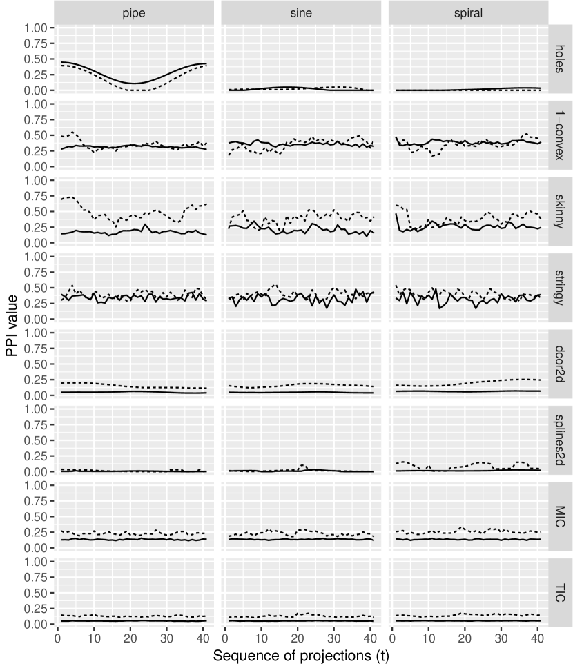
Figure 2 shows the traces representing the index values calculated across a tour between a pair of nuisance projections. The tour path is generated by interpolating between the two independent nuisance planes, i.e. from the projection onto - to one onto -. The range of each axis is set to be the limits of the index, as might be expected over many different data sets, 0 to 1. Each projection in the interpolation will also be noise. Two different sample sizes are show, as a dashed line, and as a solid line. The ideal trace is a smooth function, with relatively low values, and no difference between the sample sizes. A major feature to notice is that the scagnostics produce noisy functions, which is problematic, because small changes in the projection result in big jumps in the value. This will make them difficult to optimize. On the other hand holes, dcor2d, splines2d, MIC and TIC are relatively smooth functions.
Several of the indexes are sensitive to sample size also, the same structured projection with differing numbers of points, produces different values.
3.3 PPI traces over a tour sequence between nuisance and structured projections
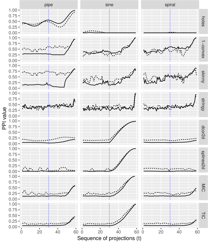
Figure 3 shows the PPIs for a tour sequence between a nuisance and structured projection. A long sequence is generated where the path interpolates between projections onto -, -, -, in order to see some of the intricacies of holes index. Sample size is indicated by line type: dashed being and solid is . The beginning of the sequence is the nuisance projection and the end is the structured projection. The index values for most PPIs increases substantially nearing the structured projection, indicating that they “see” the structure. Some indexes see all three structures: scagnostics, MIC and TIC, which means that they are flexible indexes capable of detecting a range of structure. (Grimm 2016)’s indexes, dcor2d and splines2d, are excellent for detecting the sine, and they can see it from far away, indicated by the long slow increase in index value. The holes index easily detects the pipe, and can see it from a distance, but also has local maxima along the tour path. The scagnostic index, stringy, can see the structure but is myopic, only when it is very close. Interestingly the scagnostic, skinny, sees the spiral from a distance.
3.4 Optimization check with the guided tour
Before applying the new index functions, with the guided tour on real
examples, we test them on the simulated dataset to understand the
performance of the optimization. The guided tour combines optimization
with interpolation between pairs of planes. Target planes of the path
are chosen to maximize the PPI. There are three derivative-free
optimization methods available in the guided tour:
search_better_random (1), search_better (2), and
search_geodesic (3). Method 1 casts a wide net randomly
generating projection planes, computing the PPIs and keeping the best
projection, and method 2 conducts a localized maximum search. Method 3
is quite different: a local search is conducted to determine a promising
direction, and then this direction is followed until the maximum in that
direction is found. For all methods the optimization is iterative, the
best projections form target planes in the tour, the tour path is the
interpolation to this target, and then a new search for a better
projection is made, followed by the interpolation. For each projection
during the interpolation steps, the PPI is recorded.
The stopping rule is that no better projections are found after a fixed number of tries, given a fixed tolerance value measuring difference. For method 1 and 2 two additional parameters control the optimization: the search window , giving the maximum distance from the current plane in which projections are sampled, and the cooling factor, giving the incremental decrease in search window size. Method 3 in principle also has two free parameters, which are however fixed in the current implementation. The first is the small step size used when evaluating the most promising direction, it is fixed to 0.01, and the second parameter being the window over which the line search is performed, fixed to away from the current plane.
For distributions and indexes with smooth behavior and good squintability, method 3 is the most effective method for optimization. If these two criteria are not met the method may still be useful, but only given an informed starting projection. In such cases we can follow a method similar to that proposed by Friedman (1987): we break the optimization in two distinct steps. A first step (“scouting”) uses method 2 with large search window and no cooling as a way of stepping over fluctuations and local maxima and yielding an approximation of the global maximum. Note that this likely requires large number of tries, especially as dimension increases, since most randomly picked planes will not be interesting. The second step uses method 3 starting from the approximate maximum, which will take small steps to refine the result to be closer to the global maximum.
3.4.1 Looking down the pipe
Despite the simple structure, the pipe is relatively difficult for the PPIs to find. For the TIC index, there is a fairly small squint angle. For the holes index, there are several local maxima, that divert the optimizer. There is a hint of this from Figure 3 because the initial projection (left side of trace) of purely noise variables has a higher index value than the linear combinations of noise and structured variables along the path. The uniform distribution was used to generate the noise variables, which has a higher PPI value than a normal distribution, yielding the higher initial value. In addition, a local maximum is observed whenever the pair of variables is one structured variable and one noise variable, because there is a lighter density in the center of the projection.
The optimization is done in two stages, a scouting phase using method 2, and a refinement stage using method 3. For the scouting we use and stopping condition of maximum 5000 tries, and we optimized the TIC index.
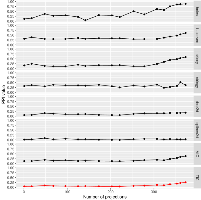
Figure 4 shows the target projections (points) selected during the scouting with method 2 on the TIC index. The focus is on the target projections rather than the interpolation between them, because the optimization is done off-line, and only the targets are used for the next step. The horizontal distance between the points in the plot reflects the relative geodesic distance between the planes in the 6D space. All of the other indexes are shown for interest. The TIC index value is generally low for this data, although it successfully detects the pipe. The holes, convex, skinny, and to some extent MIC, mirror the TIC performance. The holes differs in that it has some intermediate high values which are likely the indication of multi-modality of this index on this data.
The final views obtained in each of the two stages are compared in the Appendix.
3.4.2 Finding sine waves
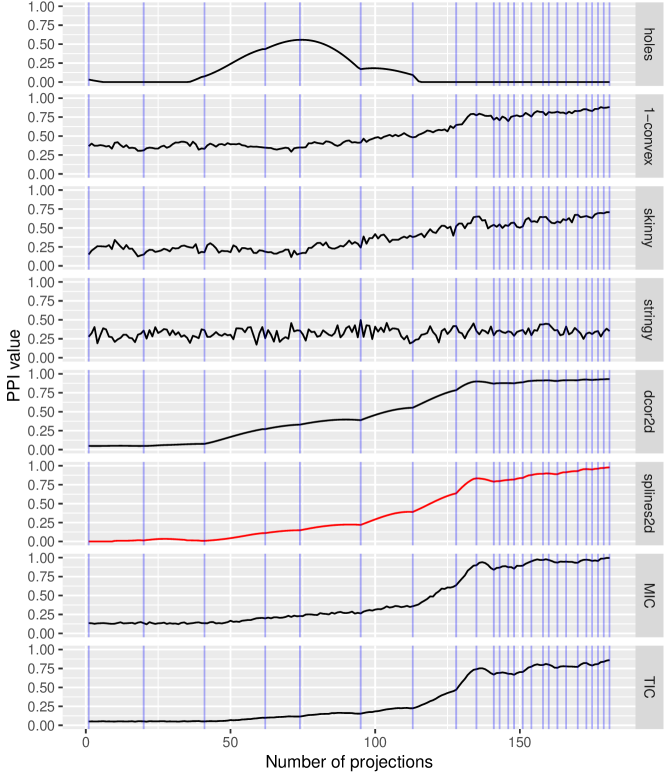
Given the patterns in Figure 3 it would be expected that the sine could be found easily, using only optimization method 3 with the splines2d, dcor2d, MIC or TIC indexes. This is examined in Figure 5. Optimization is conducted using the splines2d index, and the trace of the PPI over the optimization is shown, along with the PPI values for the other indexes over that path. The vertical blue lines indicate anchor bases, where the optimizer stops, and does a new search. The distance between anchor planes is smaller as the maximum is neared.
The only complications arise from a lack of rotation invariance of the splines2d index. It is not easily visible here, but it is possible that the best projection will have a higher PPI. The index changes depending on the basis used to define the plane, but the geodesic interpolation conducted by the tour uses any suitable basis to describe the plane, ignoring that which optimizes the PPI. This is discussed in section 3.5.
3.4.3 Spiral detection
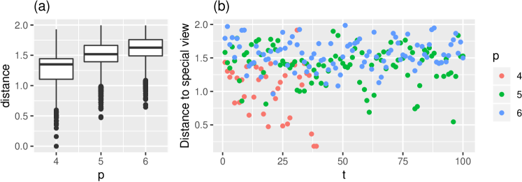
The spiral is the most challenging structure to detect because it has a small squint angle (Posse 1995b), especially as the ratio of noise to structure dimensions increases. This is explored using optimization method 2 to scout the space for approximate maxima. The skinny scagnostic index is used because it was observed (Figure 3) to be sensitive to this structure, although the noisiness of the index might be problematic. The stringy appears to be more sensitive to the spiral, but it has a much smaller squint angle.
The search is conducted for which would correspond to 2, 3 and 4 noise dimensions respectively. In addition we examine the distance between planes, using a Frobenius norm, as defined by Equation 2 of Buja et al. (2005), and available in the proj_dist function in the tourr package, to compare searches across dimensions. The distance between planes is related to squint angle, how far away from the ideal projection can the structure be glimpsed. We estimate the squint angle depending on the number of noise dimensions in the appendix. In order for the optimizer to find the spiral, the distance between planes would need to be smaller than the squint angle. Figure 6 summarizes the results. When the scouting method effectively finds the spiral. Plot (a) shows the side-by-side boxplots of pairwise distances between planes examined during the optimization, for . These are on average smaller for the lower dimension, and gradually increase as dimension increases. This is an indication of the extra computation needed to brute force find the spiral as noise dimensions increase. Plot (b) shows the distance of the plane in each iteration of the optimization to the ideal plane, where it can be seen that only when does it converge to the ideal. Its likely that expanding the search space should result in uncovering the spiral in higher dimensions, which however requires tuning of the stopping conditions and long run times.
3.5 Rotational invariance or not
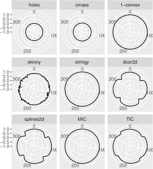
Rotational invariance is examined using the sine data (-), computing PPI for different rotations within the 2D plane, parameterized by angle. Results are shown in Figure 7. Several indexes are invariant, holes, convex and MIC, because their value is constant around rotations. The dcor2d, splines2d and TIC index are clearly not rotationally invariant because the value changes depending on the rotation. The scagnostics indexes are approximately rotationally invariant, but particularly the skinny index has some random variation depending on rotation.
3.6 Speed
Examining the computing time as a function of sample size we find that scagnostics and splines2d are fast even for large samples, while all other index functions slow rapidly with increasing sample size. Detailed results are shown in the Appendix.
3.7 Parameter choices
Some PPIs have a choice of parameters, and the choice can have an effect on function smoothness, and sensitivity to structure. In the Appendix we examine the dependence of the scagnostics indexes on the binning, showing that even with small number of bins the indexes are noisy, while they lose ability to see structure. Sensitivity to the number of bins in the MIC index is also examined, showing that tuning the parameter can improve the final result.
3.8 Index enhancement
We identified two potential improvements. First, the issue of noisy index functions may be addressed via smoothing, and we explore different smoothing options for the examples of the skinny and stringy index in the Appendix. In addition, rotation dependent indexes may be enhanced by redefining them in a rotation invariant way.
3.9 Summary
Our results can be summarized by evaluating and comparing the advantages and disadvantages of each index function according to the criteria presented above. Such an overview is given in Table 3, listing if the criteria is fully met (✓), there are some shortcomings () or failure (). (The holes index does not appear in the summary because its performance understood, and is not being examined here.) We find that none of the indexes considered meet all criteria, and in particular rotation invariance is often not fulfilled. In addition the limited flexibility of most indexes highlights the importance of index selection in the projection pursuit setup. Table 3 further suggests that there is much room for the improvement of index functions detecting unusual association between model parameters.
| Index | smooth | squintability | flexible | rotation invariant | speed |
|---|---|---|---|---|---|
| convex | ✓ | ✓ | |||
| skinny | ✓ | ||||
| stringy | ✓ | ||||
| splines2D | ✓ | ✓ | ✓ | ||
| dcor2D | ✓ | ✓ | |||
| MIC | ✓ | ✓ | |||
| TIC | ✓ | ✓ |
4 Application to physics examples
This section describes the application of these projection pursuit indices to find two-dimensional structure in two multidimensional gravitational waves problems.
The first example contains 2538 posterior samples obtained by fitting source parameters to the observed gravitational wave signal GW170817 from a neutron star merger (Abbott and others 2017). Data has been downloaded from (“LIGO” 2018). The fitting procedures are described in detail in Abbott and others (2018). We consider six parameters of physical interest (6-D) with some known relationships. Projection pursuit is used to find the known relationships.
The second example contains data generated from a simulation study of a binary black hole (BBH) merger event, as described in Smith et al. (2016). There are 12 parameters (12-D), with multiple nuisance parameters. Projection pursuit uncovers new relationships between parameters.
4.1 Neutron star merger
A scatterplot matrix (with transparency) of the six parameters is shown in the Appendix. (In astrophysics, scatterplot matrices are often called “corner plots” (Foreman-Mackey 2016).) The diagonal shows a univariate density plot of each parameter, and the upper triangle of cells displays the correlation between variables. From this it can be seen that m1 and m2 are strongly, and slightly, nonlinearly associated. Between the other variables we observe some linear association (R1, R2), some nonlinear association (L1, L2, R1, R2), heteroskedastic variance in most variables and some bimodality (R1, L1, L2, m1, m2).
The model describes a neutron star merger and contains 6 free parameters, with each neutron star described by its mass (m1, m2) and radius (R1, R2), and a so-called tidal deformability parameter (L1, L2) which is a function of the mass and radius, approximately proportional to .
4.1.1 Data pre-pocessing
Because m1 and m2 are very strongly associated, m2 is dropped before doing PP. This relationship is obvious from the scatterplots of pairs of variables and does not need to be re-discovered by PP.
All variables are scaled to range between 0 and 1. The purpose is that range differences in individual variables should not affect the detection of relationships between multiple variables. Standardizing the range will still leave differences between the standard deviations of the variables, and for this problem this is preferred. Differences in the standard deviations can be important for keeping the non-linear relationships visible to PP.
4.1.2 Applying PP
With only five parameters, a reasonable start is to examine the 5D space using a grand tour. This quickly shows the strong nonlinear relationships between the parameters. PP is then used to extract these relationships. The best index for this sort of problem is the splines2d, and it is fast to compute.
Figure 8 shows the optimal projection found by splines2d, a reconstructed view obtained by manually combining parameters, and a plot of the known relationship between parameters.

To further investigate relationships between parameters, is removed and PP with the splines2D is applied to the remaining four parameters. The dependence of on the mass and radius of the lighter neutron star, is revealed (Figure 9 left plot). A manual reconstruction shows this is a relationship between L2, R1, R2 and m1 (middle plot), but it is effectively the known relationship between L2, R2 and m2 (right plot) – m2 is latently in the relationship though m1.

4.2 Black hole simulation
This data contains posterior samples from simulation from a model describing a binary black hole (BBH) merger event. There are twelve model parameters. Flat priors are used for most model parameters.
A scatterplot matrix, of nine of the twelve parameters, is shown in the Appendix. (Parameter m2 is not shown because it is strongly linearly associated with m1, phijl and psi are not shown because they are uniform, and not associated with other parameters.) Among the nine plotted parameters, strong nonlinear relationships can be seen between the parameters ra, dec and time. The first two describe the position of the event in the sky, and time is the merging time (in GPS units). Because of the elliptical relationship between dec and time, the TIC index is used for PP, even though it is slow to compute. Between the other parameters, the main structure seen is multimodality and some skewness. These patterns are representative of the likelihood function, since most priors are flat, or built to capture growth with volume rather than distance.
4.2.1 Data pre-processing
The analysis is conducted on 11 of the twelve parameters. One variable is removed, m2, because it is so strongly associated with m1. All parameters are scaled into the range 0 to 1.
4.2.2 Applying PP
Exploring 11D with all PP indexes
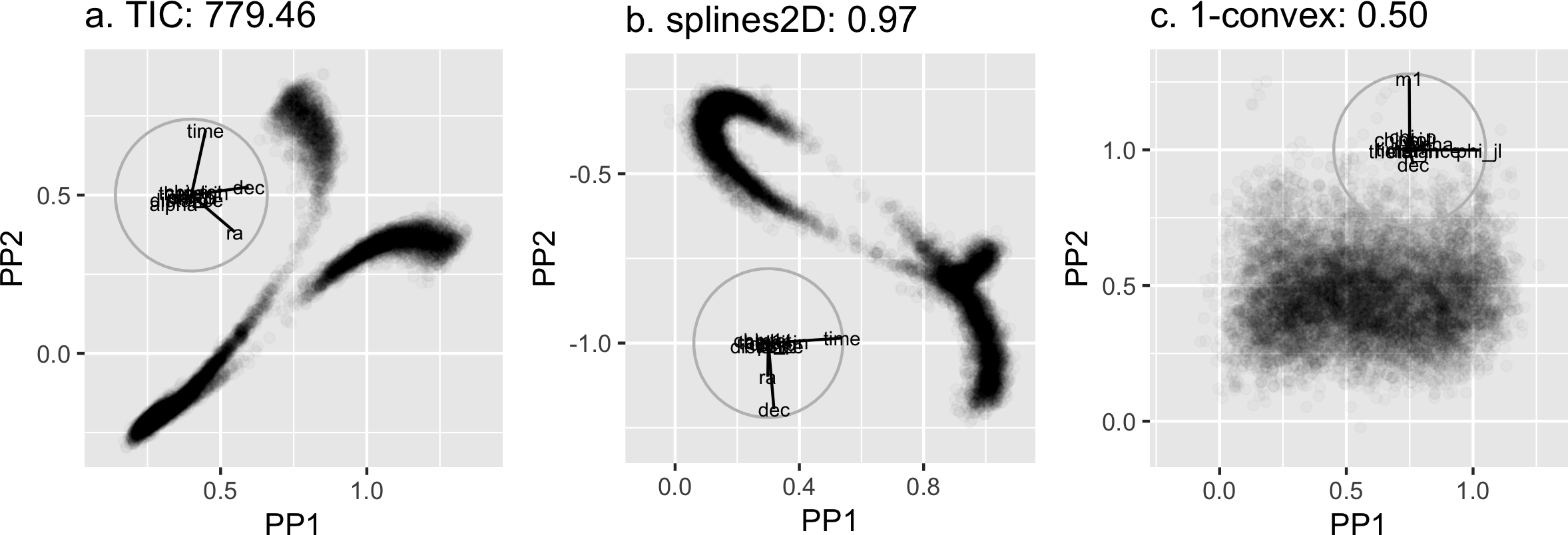
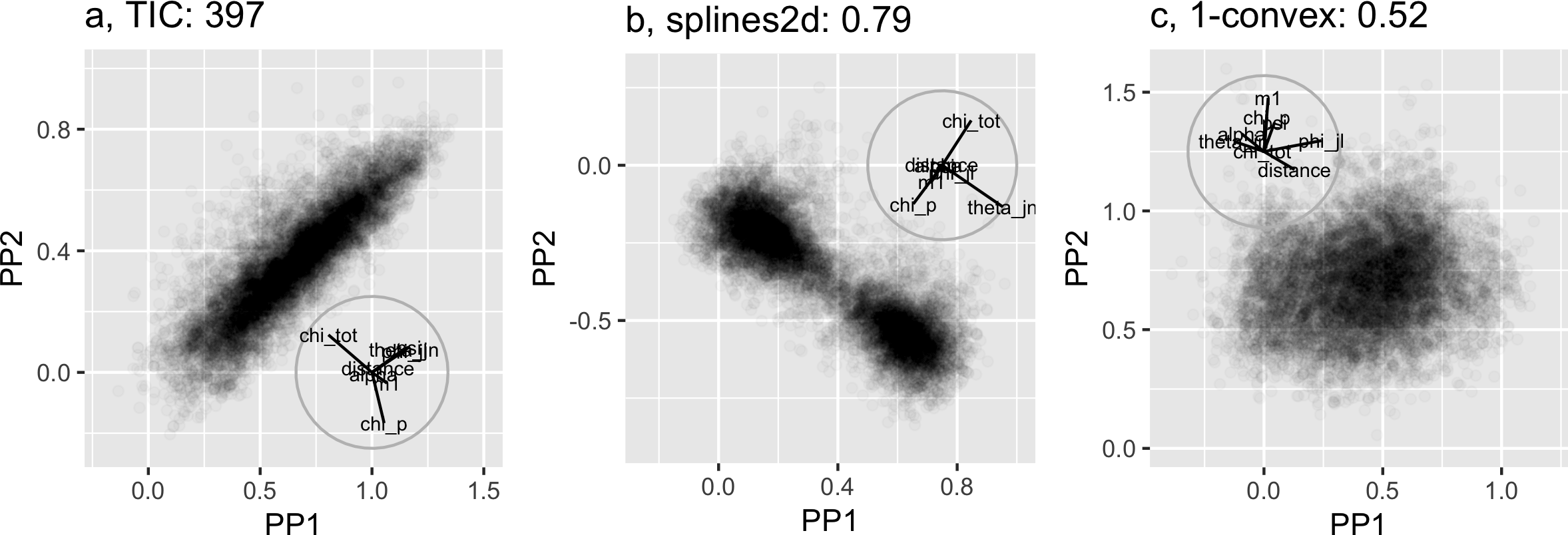
All seven PP indexes are applied to the data. Figure 10 shows the projections that maximize three of the indexes. TIC and splines2d indexes identify very similar projections, that are based on the three parameters, dec, time and ra. This is to be expected based on the pairwise scatterplots. On the other hand, the 1-convex index finds a very different view, but this is because the optimization doesn’t adequately reach a maximum for this index.
Exploring reduced space
The variables time, dec and ra are dropped from the data, and PP is applied to the remaining 8D space. Figure 11 shows the projections which maximize the TIC, splines2D and 1-convex indices. The results provide similar information as already learned from the scatterplot matrix. The parameters chitot and chip are linearly related (TIC maxima), and thetajn has a bimodal distribution yielding the figure 8 shape found by the splines2d index. The 1-convex index finds nothing interesting.
Effect of random starts, and subsets used
The initial conditions for the optimization, and the subset of variables used, can have a large effect on the projections returned. We illustrate this using only the splines2d index, and find that there is one more association that can be learned that was masked earlier.
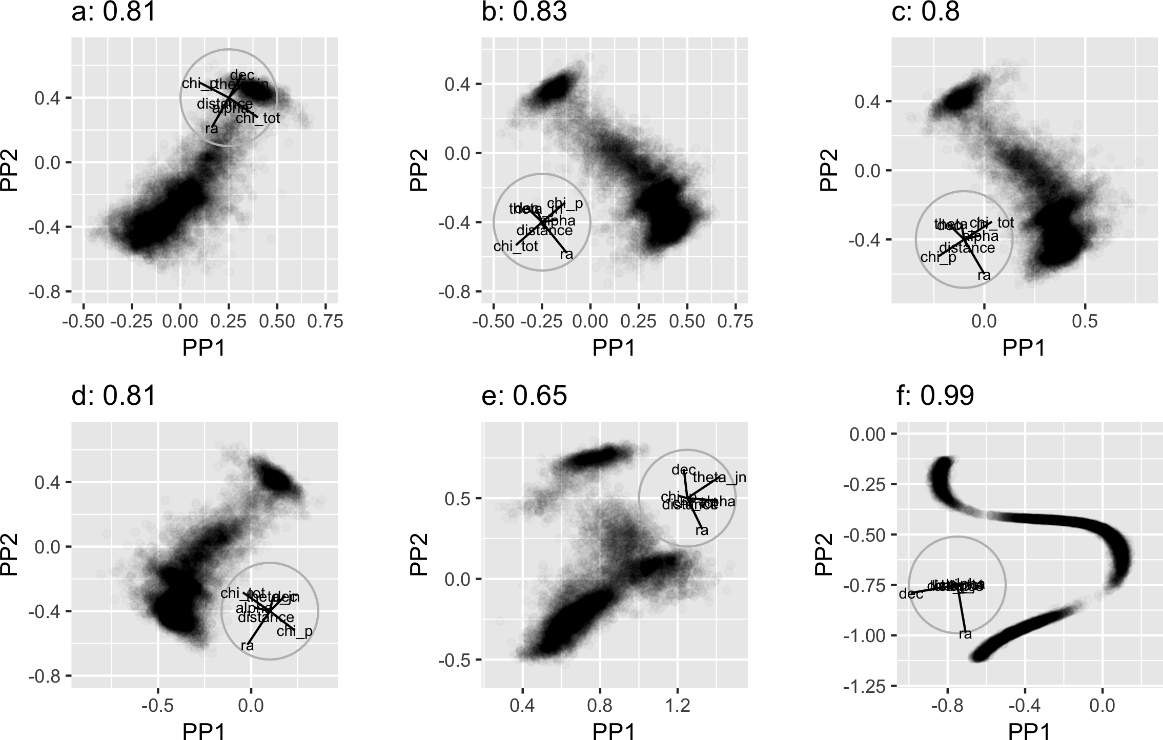
Figure 12 shows six maxima obtained by different starts, for two types of parameters: first, spin related parameters (i.e. alpha, theta_jn, chi_tot and chi_p), and second position related parameters (i.e. ra, dec and distance). Four of the six (a-d) are almost identical, but not interesting projections. Projection f has the highest PP index value but it is primarily the view seen in the bivariate plot of dec and ra. While none of these projections are particularly interesting on their own, moving between them can be revealing.
Choosing a different subset of variables reveals something new. The subspace of m1, ra, chi_tot, alpha, distance, dec produces a more refined view of Figure 12 projection f. When alpha contributes in contrast to dec, the relationship between the points is almost perfectly on a curve. This is shown in Figure 13. Manually reconstructing the optimal projection (left plot) can be done by differencing the two parameters, in their original units. This highlights the importance of improved optimization, that would use tiny final steps to polish the view to a finer optimal projection and possibly remove noise induced by small contributions of many variables.

4.3 Instructions for applying to new data
Applying these procedures to new datasets can be done using the guided tour available in the tourr package. The typical steps required are:
-
1.
Scale, standardize or sphere (principal components) the data.
-
2.
Index function selection matching the type of structure that is interesting to detect. Any new function can be used as long as it takes a matrix as input and returns a single index value.
-
3.
Call the guided tour with the data and index function:
-
•
for exploration this can be done via the tourr::animate function
-
•
for recording the results tourr::save_history should be used
-
•
-
4.
Explore how the results depend on choices made (index function, starting planes, optimization method, prior dimension reduction).
These are steps followed in the above two applications and are documented in the comments of the source code (U. Laa and Cook 2019a). For simple usage examples, see documentation of the tourr::guided_tour function.
5 Discussion
The motivation for this work was to discover dependencies between estimated parameters in multiple model fits in physics problems. This paper shows how projection pursuit with the new indexes can help address this problem. The results are encouraging, showing large potential for discovering unanticipated relations between multiple variables.
All of the indexes fall short against some aspect of the ideal properties of smoothness, squintability, flexibility, rotation invariance and speed. The paper describes how these properties can be assessed using tour methodology. Some potential fixes for the indexes are discussed but there is scope for further developing the new indexes. We recommend to use the spinebil (U. Laa and Cook 2019b) package when developing new indexes. It includes the functionalities needed to reproduce the assessments presented in this paper. While the current focus is on two-dimensional index functions, indexes in the tourr package apply to arbitrary projection dimension, and the methodology introduced here could be applied to the assessment of index functions where .
The work also reveals inadequacies in the tour optimization algorithm, that may benefit from newly developed techniques and software tools. Exploring this area would help improve the guided tours. As new optimization techniques become available, adapting these to the guided tour would extend the technique to a broader range of problems. The current recommended approach is to first reduce the dimensionality, for example by using PCA, taking care to preserve nonlinear structure, prior to applying PP.
To apply the existing index functions in practice, we recommend to either use the tourr package directly, or if interaction is required to call the guided tour via the graphical interface available in the galahr (U. Laa and Cook 2019c) package. This package supersedes the now archived tourrGui (Huang, Cook, and Wickham 2012). Both packages contain examples to show how the guided tour can be used with different index functions.
6 Supplementary material
-
•
This article was created with R Markdown (Xie, Allaire, and Grolemund 2018), the code for the paper is available at (U. Laa and Cook 2019a).
-
•
Methods for testing new index functions as presented in this work are implemented in the R package spinebil (U. Laa and Cook 2019b).
-
•
The R package galahr (U. Laa and Cook 2019c) provides a graphical interface to the tourr package allowing for interactive exploration using the guided tour.
-
•
Additional explanations are available in the Appendix, covering details of
-
–
how the holes index was rescaled,
-
–
estimations of the squint angle,
-
–
a comparison of the computational performance of the index functions,
-
–
testing the effect of index parameters on the results and
-
–
suggestions how the index functions may be refined.
-
–
Acknowledgments
The authors gratefully acknowledge the support of the Australian Research Council. We thank Rory Smith for help with the gravitational wave examples, and German Valencia for useful comments. This article was created with knitr (Xie 2015), R Markdown (Xie, Allaire, and Grolemund 2018) and bookdown (Xie 2016) with embedded code.
References
Abbott, B. P., and others. 2017. “GW170817: Observation of Gravitational Waves from a Binary Neutron Star Inspiral.” Phys. Rev. Lett. 119 (16): 161101. https://doi.org/10.1103/PhysRevLett.119.161101.
———. 2018. “GW170817: Measurements of neutron star radii and equation of state.” http://arxiv.org/abs/1805.11581.
Ahn, J. S., H. Hofmann, and D. Cook. 2003. “A Projection Pursuit Method on the Multidimensional Squared Contingency Table.” Computational Statistics 18 (3): 605–26.
Albanese, Davide, Michele Filosi, Roberto Visintainer, Samantha Riccadonna, Giuseppe Jurman, and Cesare Furlanello. 2012. “Minerva and Minepy: A c Engine for the Mine Suite and Its R, Python and Matlab Wrappers.” Bioinformatics, bts707.
Asimov, D. 1985. “The Grand Tour: A Tool for Viewing Multidimensional Data.” SIAM Journal of Scientific and Statistical Computing 6 (1): 128–43.
Buja, A., D. Cook, D. Asimov, and C. Hurley. 2005. “Computational Methods for High-Dimensional Rotations in Data Visualization.” In Handbook of Statistics: Data Mining and Visualization, edited by C. R. Rao, E. J. Wegman, and J. L. Solka, 391–413. http://www.elsevier.com: Elsevier/North Holland.
Cook, D., A. Buja, and J. Cabrera. 1992. “An Analysis of Polynomial-Based Projection Pursuit.” Computing Science and Statistics 24: 478–82.
Cook, D., A. Buja, J. Cabrera, and C. Hurley. 1995. “Grand Tour and Projection Pursuit.” Journal of Computational and Graphical Statistics 4 (3): 155–72.
Cook, Dianne, Andreas Buja, and Javier Cabrera. 1993. “Projection Pursuit Indexes Based on Orthonormal Function Expansions.” Journal of Computational and Graphical Statistics 2 (3): 225–50. http://www.jstor.org/stable/1390644.
Cook, Dianne, Ursula Laa, and German Valencia. 2018. “Dynamical projections for the visualization of PDFSense data.” Eur. Phys. J. C78 (9): 742. https://doi.org/10.1140/epjc/s10052-018-6205-2.
Cook, Dianne, and Deborah F. Swayne. 2007. Interactive and Dynamic Graphics for Data Analysis with R and Ggobi. 1st ed. Springer Publishing Company, Incorporated.
Diaconis, Persi, and David Freedman. 1984. “Asymptotics of Graphical Projection Pursuit.” Ann. Statist. 12 (3): 793–815. https://doi.org/10.1214/aos/1176346703.
Eddy, William F. 1977. “A New Convex Hull Algorithm for Planar Sets.” ACM Trans. Math. Softw. 3 (4): 398–403. https://doi.org/10.1145/355759.355766.
Edelsbrunner, H., D. Kirkpatrick, and R. Seidel. 1983. “On the Shape of a Set of Points in the Plane.” IEEE Transactions on Information Theory 29 (4): 551–59. https://doi.org/10.1109/TIT.1983.1056714.
Ferraty, F., A. Goia, E. Salinelli, and P. Vieu. 2013. “Functional Projection Pursuit Regression.” Test 22 (2): 293–320. https://search-proquest-com.ezproxy.lib.monash.edu.au/docview/1354331474?accountid=12528.
Foreman-Mackey, Daniel. 2016. “Corner.py: Scatterplot Matrices in Python.” The Journal of Open Source Software 24. https://doi.org/10.21105/joss.00024.
Friedman, J. H. 1987. “Exploratory Projection Pursuit.” Journal of the American Statistical Association 82 (1): 249–66.
Friedman, J. H., and J. W. Tukey. 1974. “A Projection Pursuit Algorithm for Exploratory Data Analysis.” IEEE Transactionson Computers 23: 881–89.
Grimm, Katrin. 2016. “Kennzahlenbasierte Grafikauswahl.” Doctoral thesis, Universität Augsburg.
———. 2017. Mbgraphic: Measure Based Graphic Selection. https://CRAN.R-project.org/package=mbgraphic.
Hall, Peter. 1989. “On Polynomial-Based Projection Indices for Exploratory Projection Pursuit.” Ann. Statist. 17 (2): 589–605. https://doi.org/10.1214/aos/1176347127.
Hofmann, Heike, Lee Wilkinson, Hadley Wickham, Duncan Temple Lang, and Anushka Anand. 2019. Binostics: Compute Scagnostics.
Hou, Siyuan, and Peter D. Wentzell. 2014. “Re-Centered Kurtosis as a Projection Pursuit Index for Multivariate Data Analysis.” Journal of Chemometrics 28 (5): 370–84. https://doi.org/10.1002/cem.2568.
Huang, Bei, Dianne Cook, and Hadley Wickham. 2012. “TourrGui: A gWidgets Gui for the Tour to Explore High-Dimensional Data Using Low-Dimensional Projections.” Journal of Statistical Software 49 (6): 1–12.
Huber, Peter J. 1985. “Projection Pursuit.” Ann. Statist. 13 (2): 435–75. https://doi.org/10.1214/aos/1176349519.
Jones, M. C., and R. Sibson. 1987. “What Is Projection Pursuit?” J. Roy. Statist. Soc., Ser. A 150: 1–36.
Kruskal, J. B. 1969. “Toward a Practical Method Which Helps Uncover the Structure of a Set of Observations by Finding the Line Transformation Which Optimizes a New ‘Index of Condensation’.” In Statistical Computation, edited by R. C. Milton and J. A. Nelder, 427–40. New York: Academic Press.
Kruskal, Joseph B. 1956. “On the Shortest Spanning Subtree of a Graph and the Traveling Salesman Problem.” Proceedings of the American Mathematical Society 7 (1): 48–50. http://www.jstor.org/stable/2033241.
Laa, U., and D. Cook. 2019a. https://github.com/uschiLaa/paper-ppi.
———. 2019b. https://github.com/uschiLaa/spinebil.
———. 2019c. https://github.com/uschiLaa/galahr.
Lee, Eun-Kyung, Dianne Cook, Sigbert Klinke, and Thomas Lumley. 2005. “Projection Pursuit for Exploratory Supervised Classification.” Journal of Computational and Graphical Statistics 14 (4): 831–46. https://doi.org/10.1198/106186005X77702.
“LIGO.” 2018. 2018. {https://dcc.ligo.org/public/0152/P1800115/005}.
Loperfido, Nicola. 2018. “Skewness-Based Projection Pursuit: A Computational Approach.” Computational Statistics & Data Analysis 120: 42–57. https://doi.org/https://doi.org/10.1016/j.csda.2017.11.001.
Marsaglia, G. 1968. “Random Numbers Fall Mainly in the Planes.” Proceedings of the National Academy of Science.
Naito, Kanta. 1997. “A Generalized Projection Pursuit Procedure and Its Significance Level.” Hiroshima Math. J. 27 (3): 513–54. https://doi.org/10.32917/hmj/1206126967.
Pan, Jian-Xin, Wing-Kam Fung, and Kai-Tai Fang. 2000. “Multiple Outlier Detection in Multivariate Data Using Projection Pursuit Techniques.” Journal of Statistical Planning and Inference 83 (1): 153–67. https://doi.org/https://doi.org/10.1016/S0378-3758(99)00091-9.
Pilhöfer, Alexander, and Antony Unwin. 2013. “New Approaches in Visualization of Categorical Data: R Package extracat.” Journal of Statistical Software 53 (7): 1–25. http://www.jstatsoft.org/v53/i07/.
Posse, Christian. 1995a. “Projection Pursuit Exploratory Data Analysis.” Computational Statistics & Data Analysis 20 (6): 669–87. https://doi.org/https://doi.org/10.1016/0167-9473(95)00002-8.
———. 1995b. “Tools for Two-Dimensional Exploratory Projection Pursuit.” Journal of Computational and Graphical Statistics 4 (2): 83–100. http://www.jstor.org/stable/1390759.
R Core Team. 2018. R: A Language and Environment for Statistical Computing. Vienna, Austria: R Foundation for Statistical Computing. https://www.R-project.org/.
Reshef, David N., Yakir A. Reshef, Hilary K. Finucane, Sharon R. Grossman, Gilean McVean, Peter J. Turnbaugh, Eric S. Lander, Michael Mitzenmacher, and Pardis C. Sabeti. 2011. “Detecting Novel Associations in Large Data Sets.” Science 334 (6062): 1518–24. https://doi.org/10.1126/science.1205438.
Reshef, Yakir A., David N. Reshef, Hilary K. Finucane, Pardis C. Sabeti, and Michael Mitzenmacher. 2016. “Measuring Dependence Powerfully and Equitably.” Journal of Machine Learning Research 17 (212): 1–63. http://jmlr.org/papers/v17/15-308.html.
Rodriguez-Martinez, E., J. Yannis Goulermas, T. Mu, and J. F. Ralph. 2010. “Automatic Induction of Projection Pursuit Indices.” IEEE Transactions on Neural Networks 21 (8): 1281–95. https://doi.org/10.1109/TNN.2010.2051161.
Simon, Noah, and Robert Tibshirani. 2014. “Comment on ‘Detecting Novel Associations In Large Data Sets’ by Reshef Et Al, Science Dec 16, 2011.” arXiv E-Prints, January, arXiv:1401.7645. http://arxiv.org/abs/1401.7645.
Smith, Rory, Scott E. Field, Kent Blackburn, Carl-Johan Haster, Michael Pürrer, Vivien Raymond, and Patricia Schmidt. 2016. “Fast and accurate inference on gravitational waves from precessing compact binaries.” Phys. Rev. D94 (4): 044031. https://doi.org/10.1103/PhysRevD.94.044031.
Székely, Gábor J., Maria L. Rizzo, and Nail K. Bakirov. 2007. “Measuring and Testing Dependence by Correlation of Distances.” Ann. Statist. 35 (6): 2769–94. https://doi.org/10.1214/009053607000000505.
Tukey, P.A., and J.W. Tukey. 1981. Graphical Display of Data in Three and Higher Dimensions. Wiley Series in Probability and Mathematical Statistics: Applied Probability and Statistics. Wiley. https://books.google.com.au/books?id=WBzvAAAAMAAJ.
Wahba, G. 1990. Spline Models for Observational Data. CBMS-Nsf Regional Conference Series in Applied Mathematics. Society for Industrial; Applied Mathematics. https://books.google.com.au/books?id=ScRQJEETs0EC.
Wickham, Hadley, Dianne Cook, Heike Hofmann, and Andreas Buja. 2011. “tourr: An R Package for Exploring Multivariate Data with Projections.” Journal of Statistical Software 40 (2): 1–18. http://www.jstatsoft.org/v40/i02/.
Wilkinson, L., A. Anand, and R. Grossman. 2005. “Graph-Theoretic Scagnostics.” In IEEE Symposium on Information Visualization, 2005. INFOVIS 2005., 157–64. https://doi.org/10.1109/INFVIS.2005.1532142.
Wilkinson, Leland, and Graham Wills. 2008. “Scagnostics Distributions.” Journal of Computational and Graphical Statistics 17 (2): 473–91. https://doi.org/10.1198/106186008X320465.
Wood, S.N., N., Pya, and B. Säfken. 2016. “Smoothing Parameter and Model Selection for General Smooth Models (with Discussion).” Journal of the American Statistical Association 111: 1548–75.
Xie, Yihui. 2015. Dynamic Documents with R and Knitr. 2nd ed. Boca Raton, Florida: Chapman; Hall/CRC. https://yihui.name/knitr/.
———. 2016. Bookdown: Authoring Books and Technical Documents with R Markdown. Boca Raton, Florida: Chapman; Hall/CRC. https://github.com/rstudio/bookdown.
Xie, Yihui, J.J. Allaire, and Garrett Grolemund. 2018. R Markdown: The Definitive Guide. Boca Raton, Florida: Chapman; Hall/CRC. https://bookdown.org/yihui/rmarkdown.