A Geometric Perspective on Optimal Representations for Reinforcement Learning
Abstract
We propose a new perspective on representation learning in reinforcement learning based on geometric properties of the space of value functions. We leverage this perspective to provide formal evidence regarding the usefulness of value functions as auxiliary tasks. Our formulation considers adapting the representation to minimize the (linear) approximation of the value function of all stationary policies for a given environment. We show that this optimization reduces to making accurate predictions regarding a special class of value functions which we call adversarial value functions (AVFs). We demonstrate that using value functions as auxiliary tasks corresponds to an expected-error relaxation of our formulation, with AVFs a natural candidate, and identify a close relationship with proto-value functions (Mahadevan, 2005). We highlight characteristics of AVFs and their usefulness as auxiliary tasks in a series of experiments on the four-room domain.
1 Introduction
00footnotetext: 1Google Brain 2DeepMind 3Mila, Université de Montréal 4University of Alberta 5University of OxfordA good representation of state is key to practical success in reinforcement learning. While early applications used hand-engineered features (Samuel,, 1959), these have proven onerous to generate and difficult to scale. As a result, methods in representation learning have flourished, ranging from basis adaptation (Menache et al.,, 2005; Keller et al.,, 2006), gradient-based learning (Yu and Bertsekas,, 2009), proto-value functions (Mahadevan and Maggioni,, 2007), feature generation schemes such as tile coding (Sutton,, 1996) and the domain-independent features used in some Atari 2600 game-playing agents (Bellemare et al.,, 2013; Liang et al.,, 2016), and nonparametric methods (Ernst et al.,, 2005; Farahmand et al.,, 2016; Tosatto et al.,, 2017). Today, the method of choice is deep learning. Deep learning has made its mark by showing it can learn complex representations of relatively unprocessed inputs using gradient-based optimization (Tesauro,, 1995; Mnih et al.,, 2015; Silver et al.,, 2016).
Most current deep reinforcement learning methods augment their main objective with additional losses called auxiliary tasks, typically with the aim of facilitating and regularizing the representation learning process. The UNREAL algorithm, for example, makes predictions about future pixel values (Jaderberg et al.,, 2017); recent work approximates a one-step transition model to achieve a similar effect (François-Lavet et al.,, 2018; Gelada et al.,, 2019). The good empirical performance of distributional reinforcement learning (Bellemare et al.,, 2017) has also been attributed to representation learning effects, with recent visualizations supporting this claim (Such et al.,, 2019). However, while there is now conclusive empirical evidence of the usefulness of auxiliary tasks, their design and justification remain on the whole ad-hoc. One of our main contributions is to provides a formal framework in which to reason about auxiliary tasks in reinforcement learning.
We begin by formulating an optimization problem whose solution is a form of optimal representation. Specifically, we seek a state representation from which we can best approximate the value function of any stationary policy for a given Markov Decision Process. Simultaneously, the largest approximation error in that class serves as a measure of the quality of the representation. While our approach may appear naive – in real settings, most policies are uninteresting and hence may distract the representation learning process – we show that our representation learning problem can in fact be restricted to a special subset of value functions which we call adversarial value functions (AVFs). We then characterize these adversarial value functions and show they correspond to deterministic policies that either minimize or maximize the expected return at each state, based on the solution of a network-flow optimization derived from an interest function .
A consequence of our work is to formalize why predicting value function-like objects is helpful in learning representations, as has been argued in the past (Sutton et al.,, 2011, 2016). We show how using these predictions as auxiliary tasks can be interpreted as a relaxation of our optimization problem. From our analysis, we hypothesize that auxiliary tasks that resemble adversarial value functions should give rise to good representations in practice. We complement our theoretical results with an empirical study in a simple grid world environment, focusing on the use of deep learning techniques to learn representations. We find that predicting adversarial value functions as auxiliary tasks leads to rich representations.
2 Setting
We consider an environment described by a Markov Decision Process (Puterman,, 1994); and are finite state and action spaces, is the transition function, the discount factor, and the reward function. For a finite set , write for the probability simplex over . A (stationary) policy is a mapping , also denoted . We denote the set of policies by . We combine a policy with the transition function to obtain the state-to-state transition function . The value function describes the expected discounted sum of rewards obtained by following :
The value function satisfies Bellman’s equation (Bellman,, 1957): . We will find it convenient to use vector notation: Assuming there are states, we view and as vectors in and , yielding
A -dimensional representation is a mapping ; is the feature vector for state . We write to denote the matrix whose rows are , and with some abuse of notation denote the set of -dimensional representations by . For a given representation and weight vector , the linear approximation for a value function is
We consider the approximation minimizing the uniformly weighted squared error
We denote by the projection of onto the linear subspace .
2.1 Two-Part Approximation
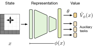
We view as a two-part approximation arising from the composition of an adjustable representation and a weight vector ; we use the term “two-part” to emphasize that the mapping is linear, while itself may not be. This separation into two parts gives us a simple framework in which to study the behaviour of representation learning, in particular deep networks applied to reinforcement learning. We will further consider the use of to make additional predictions, called auxiliary tasks following common usage, and whose purpose is to improve or stabilize the representation.
We study two-part approximations in an idealized setting where the length of is fixed and smaller than , but the mapping is otherwise unconstrained. Even this idealized design offers interesting problems to study. We might be interested in sharing a representation across problems, as is often done in transfer or continual learning. In this context, auxiliary tasks may inform how the value function should generalize to these new problems. In many problems of interest, the weights can also be optimized more efficiently than the representation itself, warranting the view that the representation should be adapted using a different process (Levine et al.,, 2017; Chung et al.,, 2019).
Note that a trivial “value-as-feature” representation exists for the single-policy optimization problem
this approximation sets . In this paper we take the stance that this is not a satisfying representation, and that a good representation should be in the service of a broader goal (e.g. control, transfer, or fairness).
3 Representation Learning by Approximating Value Functions
We measure the quality of a representation in terms of how well it can approximate all possible value functions, formalized as the representation error
We consider the problem of finding the representation minimizing :
| (1) |
In the context of our work, we call this the representation learning problem (rlp) and say that a representation is optimal when it minimizes the error in (1). Note that (and hence ) depends on characteristics of the environment, in particular on both reward and transition functions.
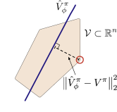
We consider the rlp from a geometric perspective (Figure 1, right). Dadashi et al., (2019) showed that the set of value functions achieved by the set of policies , denoted
forms a (possibly nonconvex) polytope. As previously noted, a given representation defines a linear subspace of possible value approximations. The maximal error is achieved by the value function in which is furthest along the subspace normal to , since is the orthogonal projection of .
We say that is an extremal vertex if it is a vertex of the convex hull of . Our first result shows that for any direction , the furthest point in along is an extremal vertex, and is in general unique for this (proof in the appendix).
Lemma 1.
Let and define the functional , with domain . Then is maximized by an extremal vertex , and there is a deterministic policy for which . Furthermore, the set of directions for which the maximum of is achieved by multiple extremal vertices has Lebesgue measure zero in .
Denote by the set of policies corresponding to extremal vertices of . We next derive an equivalence between the rlp and an optimization problem which only considers policies in .
Theorem 1.
For any representation , the maximal approximation error measured over all value functions is the same as the error measured over the set of extremal vertices:
Theorem 1 indicates that we can find an optimal representation by considering a finite (albeit exponential) number of value functions, since each extremal vertex corresponds to the value function of some deterministic policy, of which there are at most an exponential number. We will call these adversarial value functions (AVFs), because of the minimax flavour of the rlp.
Solving the rlp allows us to provide quantifiable guarantees on the performance of certain value-based learning algorithms. For example, in the context of least-squares policy iteration (LSPI; Lagoudakis and Parr,, 2003), minimizing the representation error directly improves the performance bound. By contrast, we cannot have the same guarantee if is learned by minimizing the approximation error for a single value function.
Corollary 1.
Let be an optimal representation in the rlp. Consider the sequence of policies derived from LSPI using to approximate under a uniform sampling of the state-space. Then there exists an MDP-dependent constant such that
This result is a direct application of the quadratic norm bounds given by Munos, (2003), in whose work the constant is made explicit. We emphasize that the result is illustrative; our approach should enable similar guarantees in other contexts (e.g. Munos,, 2007; Petrik and Zilberstein,, 2011).
3.1 The Structure of Adversarial Value Functions
The rlp suggests that an agent trained to predict various value functions should develop a good state representation. Intuitively, one may worry that there are simply too many “uninteresting” policies, and that a representation learned from their value functions emphasizes the wrong quantities. However, the search for an optimal representation is closely tied to the much smaller set of adversarial value functions (AVFs). The aim of this section is to characterize the structure of AVFs and show that they form an interesting subset of all value functions. From this, we argue that their use as auxiliary tasks should also produce structured representations.
From Lemma 1, recall that an AVF is geometrically defined using a vector and the functional , which the AVF maximizes. Since is restricted to the value polytope, we can consider the equivalent policy-space functional . Observe that
| (2) |
In this optimization problem, the vector defines a weighting over the state space ; for this reason, we call an interest function in the context of AVFs. Whenever componentwise, we recover the optimal value function, irrespective of the exact magnitude of (Bertsekas,, 2012). If for some , however, the maximization becomes a minimization. As the next result shows, the policy maximizing depends on a network flow derived from and the transition function .
Theorem 2.
Maximizing the functional is equivalent to finding a network flow that satisfies a reverse Bellman equation:
For a policy maximizing the above we have
Corollary 2.
There are at most distinct adversarial value functions.
The vector corresponds to the sum of discounted interest weights flowing through a state , similar to the dual variables in the theory of linear programming for MDPs (Puterman,, 1994). Theorem 2, by way of the corollary, implies that there are fewer AVFs () than deterministic policies (. It also implies that AVFs relate to a reward-driven purpose, similar to how the optimal value function describes the goal of maximizing return. We will illustrate this point empirically in Section 4.1.
3.2 Relationship to Auxiliary Tasks
So far we have argued that solving the rlp leads to a representation which is optimal in a meaningful sense. However, solving the rlp seems computationally intractable: there are an exponential number of deterministic policies to consider (Prop. 1 in the appendix gives a quadratic formulation with quadratic constraints). Using interest functions does not mitigate this difficulty: the computational problem of finding the AVF for a single interest function is NP-hard, even when restricted to deterministic MDPs (Prop. 2 in the appendix).
Instead, in this section we consider a relaxation of the rlp and show that this relaxation describes existing representation learning methods, in particular those that use auxiliary tasks. Let be some distribution over . We begin by replacing the maximum in (1) by an expectation:
| (3) |
The use of the expectation offers three practical advantages over the use of the maximum. First, this leads to a differentiable objective which can be minimized using deep learning techniques. Second, the choice of gives us an additional degree of freedom; in particular, needs not be restricted to the value polytope. Third, the minimizer in (3) is easily characterized, as the following theorem shows.
Theorem 3.
One may expect the quality of the learned representation to depend on how closely the distribution relates to the rlp. From an auxiliary tasks perspective, this corresponds to choosing tasks that are in some sense useful. For example, generating value functions from the uniform distribution over the set of policies , while a natural choice, may put too much weight on “uninteresting” value functions.
In practice, we may further restrict to a finite set . Under a uniform weighting, this leads to a representation loss
| (4) |
which corresponds to the typical formulation of an auxiliary-task loss (e.g. Jaderberg et al.,, 2017). In a deep reinforcement learning setting, one typically minimizes (4) using stochastic gradient descent methods, which scale better than batch methods such as singular value decomposition (but see Wu et al., (2019) for further discussion).
Our analysis leads us to conclude that, in many cases of interest, the use of auxiliary tasks produces representations that are close to the principal components of the set of tasks under consideration. If is well-aligned with the rlp, minimizing should give rise to a reasonable representation. To demonstrate the power of this approach, in Section 4 we will study the case when the set is constructed by sampling AVFs – emphasizing the policies that support the solution to the rlp.
3.3 Relationship to Proto-Value Functions
Proto-value functions (Mahadevan and Maggioni,, 2007, pvf) are a family of representations which vary smoothly across the state space. Although the original formulation defines this representation as the largest-eigenvalue eigenvectors of the Laplacian of the transition function’s graphical structure, recent formulations use the top singular vectors of , where is the uniformly random policy (Stachenfeld et al.,, 2014; Machado et al.,, 2017; Behzadian and Petrik,, 2018).
In line with the analysis of the previous section, proto-value functions can also be interpreted as defining a set of value-based auxiliary tasks. Specifically, if we define an indicator reward function and a set of value functions with the uniformly random policy, then any -dimensional representation that minimizes (4) spans the same basis as the -dimensional pvf (up to the bias term). This suggests a connection with hindsight experience replay (Andrychowicz et al.,, 2017), whose auxiliary tasks consists in reaching previously experienced states.
4 Empirical Studies
In this section we complement our theoretical analysis with an experimental study. In turn, we take a closer look at 1) the structure of adversarial value functions, 2) the shape of representations learned using AVFs, and 3) the performance profile of these representations in a control setting.
Our eventual goal is to demonstrate that the representation learning problem (1), which is based on approximating value functions, gives rise to representations that are both interesting and comparable to previously proposed schemes. Our concrete instantiation (Algorithm 1) uses the representation loss (4). As-is, this algorithm is of limited practical relevance (our AVFs are learned using a tabular representation) but we believe provides an inspirational basis for further developments.
We perform all of our experiments within the four-room domain (Sutton et al.,, 1999; Solway et al.,, 2014; Machado et al.,, 2017, Figure 2, see also Appendix H.1).
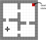

We consider a two-part approximation where we pretrain end-to-end to predict a set of value functions. Our aim here is to compare the effects of using different sets of value functions, including AVFs, on the learned representation. As our focus is on the efficient use of a -dimensional representation (with , the number of states), we encode individual states as one-hot vectors and map them into without capacity constraints. Additional details may be found in Appendix H.
4.1 Adversarial Value Functions
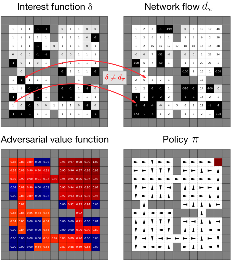
Our first set of results studies the structure of adversarial value functions in the four-room domain. We generated interest functions by assigning a value uniformly at random to each state (Figure 2, left). We restricted to these discrete choices for illustrative purposes.
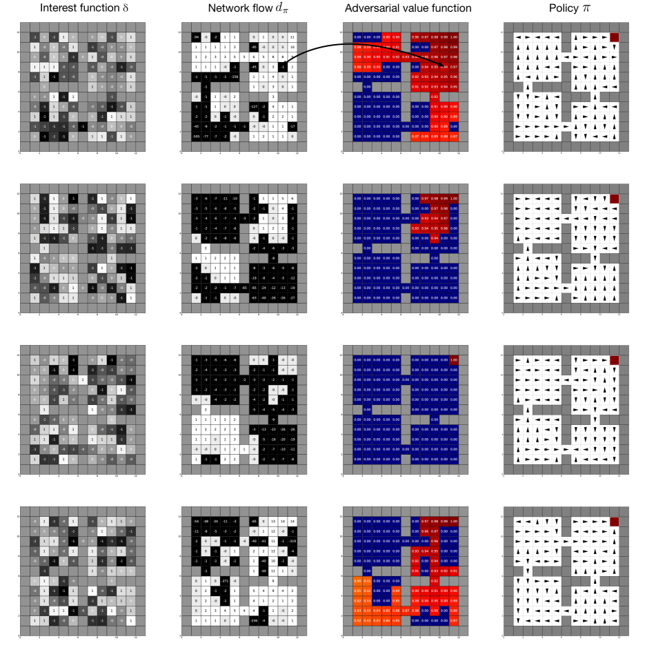
We then used model-based policy gradient (Sutton et al.,, 2000) to find the policy maximizing . We observed some local minima or accumulation points but as a whole reasonable solutions were found. The resulting network flow and AVF for a particular sample are shown in Figure 2. For most states, the signs of and agree; however, this is not true of all states (larger version and more examples in appendix, Figures 6, 7). As expected, states for which (respectively, ) correspond to states maximizing (resp. minimizing) the value function. Finally, we remark on the “flow” nature of : trajectories over minimizing states accumulate in corners or loops, while those over maximizing states flow to the goal. We conclude that AVFs exhibit interesting structure, and are generated by policies that are not random (Figure 2, right). As we will see next, this is a key differentiator in making AVFs good auxiliary tasks.
4.2 Representation Learning with AVFs
We next consider the representations that arise from training a deep network to predict AVFs (denoted avf from here on). We sample interest functions and use Algorithm 1 to generate AVFs. We combine these AVFs into the representation loss (4) and adapt the parameters of the deep network using Rmsprop (Tieleman and Hinton,, 2012).
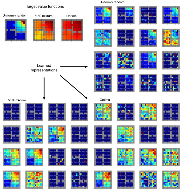
We contrast the AVF-driven representation with one learned by predicting the value function of random deterministic policies (rp). Specifically, these policies are generated by assigning an action uniformly at random to each state. We also consider the value function of the uniformly random policy (value). While we make these choices here for concreteness, other experiments yielded similar results (e.g. predicting the value of the optimal policy; appendix, Figure 8). In all cases, we learn a dimensional representation, not including the bias unit.

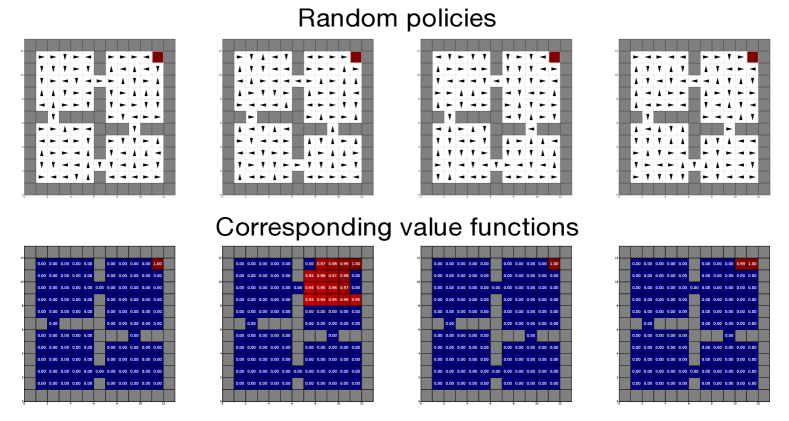
Figure 3 shows the representations learned by the three methods. The features learned by value resemble the value function itself (top left feature) or its negated image (bottom left feature). Coarsely speaking, these features capture the general distance to the goal but little else. The features learned by rp are of even worse quality. This is because almost all random deterministic policies cause the agent to avoid the goal (appendix, Figure 12). The representation learned by avf, on the other hand, captures the structure of the domain, including paths between distal states and focal points corresponding to rooms or parts of rooms.
Although our focus is on the use of AVFs as auxiliary tasks to a deep network, we observe the same results when discovering a representation using singular value decomposition (Section 3.2), as described in Appendix I. All in all, our results illustrate that, among all value functions, AVFs are particularly useful auxiliary tasks for representation learning.
4.3 Learning the Optimal Policy
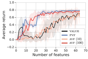
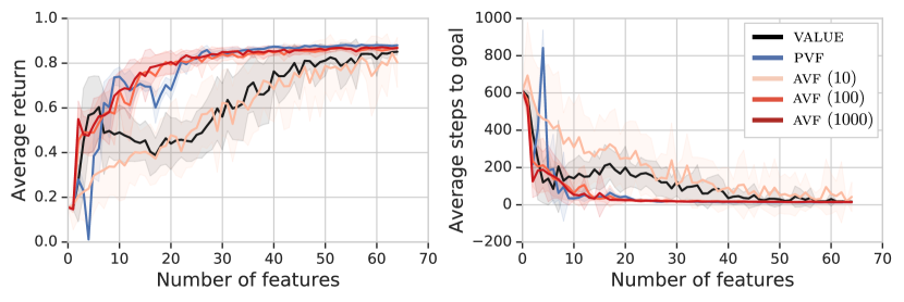
In a final set of experiments, we consider learning a reward-maximizing policy using a pretrained representation and a model-based version of the SARSA algorithm (Rummery and Niranjan,, 1994; Sutton and Barto,, 1998). We compare the value-based and AVF-based representations from the previous section (value and avf), and also proto-value functions (pvf; details in Appendix H.3).
We report the quality of the learned policies after training, as a function of , the size of the representation. Our quality measures is the average return from the designated start state (bottom left). Results are provided in Figure 4 and Figure 13 (appendix). We observe a failure of the value representation to provide a useful basis for learning a good policy, even as increases; while the representation is not rank-deficient, the features do not help reduce the approximation error. In comparison, our avf representations perform similarly to pvfs. Increasing the number of auxiliary tasks also leads to better representations; recall that pvf implicitly uses auxiliary tasks.
5 Related Work
Our work takes inspiration from earlier research in basis or feature construction for reinforcement learning. Ratitch and Precup, (2004), Foster and Dayan, (2002), Menache et al., (2005), Yu and Bertsekas, (2009), Bhatnagar et al., (2013), and Song et al., (2016) consider methods for adapting parametrized basis functions using iterative schemes. Including Mahadevan and Maggioni, (2007)’s proto-value functions, a number of works (we note Dayan,, 1993; Petrik,, 2007; Mahadevan and Liu,, 2010; Ruan et al.,, 2015; Barreto et al.,, 2017) have used characteristics of the transition structure of the MDP to generate representations; these are the closest in spirit to our approach, although none use the reward or consider the geometry of the space of value functions. Parr et al., (2007) proposed constructing a representation from successive Bellman errors, Keller et al., (2006) used dimensionality reduction methods; finally Hutter, (2009) proposes a universal scheme for selecting representations.
Deep reinforcement learning algorithms have made extensive use of auxiliary tasks to improve agent performance, beginning perhaps with universal value function approximators (Schaul et al.,, 2015) and the UNREAL architecture (Jaderberg et al.,, 2017); see also Dosovitskiy and Koltun, (2017), François-Lavet et al., (2018) and, more tangentially, van den Oord et al., (2018). Levine et al., (2017) and Chung et al., (2019) make explicit use of two-part approximations to derive more sample efficient deep reinforcement learning algorithms. The notion of augmenting an agent with side predictions regarding the world is not new, with roots in TD models (Sutton,, 1995), predictive state representations (Littman et al.,, 2002) and the Horde architecture (Sutton et al.,, 2011), which itself is based on Selfridge, (1959)’s Pandemonium architecture.
In passing, we remark on a number of works which aim to quantify or explain the usefulness of a representation. Parr et al., (2008) studies the particular case of linear representations, while Li et al., (2006); Abel et al., (2016) consider the approximation error that arises from state abstraction. More recently, Nachum et al., (2019) provide some interesting guarantees in the context of hierarchical reinforcement learning, while Such et al., (2019) visualizes the representations learned by Atari-playing agents. Finally, Bertsekas, (2018) remarks on the two-part approximation we study here.
6 Conclusion
In this paper we studied the notion of an adversarial value function, derived from a geometric perspective on representation learning in RL. Our work shows that adversarial value functions exhibit interesting structure, and are good auxiliary tasks when learning a representation of an environment. We believe our work to be the first to provide formal evidence as to the usefulness of predicting value functions for shaping an agent’s representation.
Our work opens up the possibility of automatically generating auxiliary tasks in deep reinforcement learning, analogous to how deep learning itself enabled a move away from hand-crafted features. A number of practical considerations remain to be addressed. First, our sampling procedure is clearly inefficient, and may be improved by encouraging diversity within AVFs. Second, practical implementations require learning the AVFs concurrently with the main task. Doing results in off-policy learning, whose negative effects are well-documented even in recent applications. (e.g. van Hasselt et al.,, 2018). Third, interest functions in large domains should incorporate some degree of smoothness, rather than vary rapidly from state to state.
From a mathematical perspective, our formulation of the representation learning problem (1) was made with both convenience and geometry in mind. Conceptually, it may be interesting to consider our approach in other norms, including the weighted norms used in approximation results.
7 Acknowledgements
The authors thank the many people who helped shape this project through discussions and feedback on early drafts: Lihong Li, George Tucker, Doina Precup, Ofir Nachum, Csaba Szepesvári, Georg Ostrovski, Marek Petrik, Marlos Machado, Tim Lillicrap, Danny Tarlow, Saurabh Kumar, and Carles Gelada. Special thanks also to Philip Thomas and Scott Niekum, who gave this project its initial impetus.
8 Author Contributions
M.G.B., W.D., D.S., and N.L.R. conceptualized the representation learning problem. M.G.B., W.D., T.L., A.A.T., R.D., D.S., and N.L.R. contributed to the theoretical results. M.G.B., W.D., P.S.C., R.D., and C.L. performed experiments and collated results. All authors contributed to the writing.
References
- Abadi et al., (2016) Abadi, M., Barham, P., Chen, J., Chen, Z., Davis, A., Dean, J., Devin, M., Ghemawat, S., Irving, G., Isard, M., et al. (2016). Tensorflow: A system for large-scale machine learning. In Symposium on Operating Systems Design and Implementation.
- Abel et al., (2016) Abel, D., Hershkowitz, D. E., and Littman, M. L. (2016). Near optimal behavior via approximate state abstraction. In Proceedings of the International Conference on Machine Learning.
- Andrychowicz et al., (2017) Andrychowicz, M., Wolski, F., Ray, A., Schneider, J., Fong, R., Welinder, P., McGrew, B., Tobin, J., Abbeel, O. P., and Zaremba, W. (2017). Hindsight experience replay. In Advances in Neural Information Processing Systems.
- Barreto et al., (2017) Barreto, A., Dabney, W., Munos, R., Hunt, J. J., Schaul, T., van Hasselt, H. P., and Silver, D. (2017). Successor features for transfer in reinforcement learning. In Advances in Neural Information Processing Systems.
- Behzadian and Petrik, (2018) Behzadian, B. and Petrik, M. (2018). Feature selection by singular value decomposition for reinforcement learning. In Proceedings of the ICML Prediction and Generative Modeling Workshop.
- Bellemare et al., (2017) Bellemare, M. G., Dabney, W., and Munos, R. (2017). A distributional perspective on reinforcement learning. In Proceedings of the International Conference on Machine Learning.
- Bellemare et al., (2013) Bellemare, M. G., Naddaf, Y., Veness, J., and Bowling, M. (2013). The Arcade Learning Environment: An evaluation platform for general agents. Journal of Artificial Intelligence Research, 47:253–279.
- Bellman, (1957) Bellman, R. E. (1957). Dynamic programming. Princeton University Press, Princeton, NJ.
- Bernhard and Vygen, (2008) Bernhard, K. and Vygen, J. (2008). Combinatorial optimization: Theory and algorithms. Springer, Third Edition, 2005.
- Bertsekas, (2012) Bertsekas, D. P. (2012). Dynamic Programming and Optimal Control, Vol. II: Approximate Dynamic Programming. Athena Scientific.
- Bertsekas, (2018) Bertsekas, D. P. (2018). Feature-based aggregation and deep reinforcement learning: A survey and some new implementations. Technical report, MIT/LIDS.
- Bhatnagar et al., (2013) Bhatnagar, S., Borkar, V. S., and Prabuchandran, K. (2013). Feature search in the Grassmanian in online reinforcement learning. IEEE Journal of Selected Topics in Signal Processing.
- Boyd and Vandenberghe, (2004) Boyd, S. and Vandenberghe, L. (2004). Convex optimization. Cambridge university press.
- Castro et al., (2018) Castro, P. S., Moitra, S., Gelada, C., Kumar, S., and Bellemare, M. G. (2018). Dopamine: A research framework for deep reinforcement learning. arXiv.
- Chung et al., (2019) Chung, W., Nath, S., Joseph, A. G., and White, M. (2019). Two-timescale networks for nonlinear value function approximation. In International Conference on Learning Representations.
- Dadashi et al., (2019) Dadashi, R., Taïga, A. A., Roux, N. L., Schuurmans, D., and Bellemare, M. G. (2019). The value function polytope in reinforcement learning. arXiv.
- Dayan, (1993) Dayan, P. (1993). Improving generalisation for temporal difference learning: The successor representation. Neural Computation.
- Dosovitskiy and Koltun, (2017) Dosovitskiy, A. and Koltun, V. (2017). Learning to act by predicting the future. In Proceedings of the International Conference on Learning Representations.
- Ernst et al., (2005) Ernst, D., Geurts, P., and Wehenkel, L. (2005). Tree-based batch mode reinforcement learning. Journal of Machine Learning Research, 6:503–556.
- Farahmand et al., (2016) Farahmand, A., Ghavamzadeh, M., Szepesvári, C., and Mannor, S. (2016). Regularized policy iteration with nonparametric function spaces. Journal of Machine Learning Research.
- Foster and Dayan, (2002) Foster, D. and Dayan, P. (2002). Structure in the space of value functions. Machine Learning.
- François-Lavet et al., (2018) François-Lavet, V., Bengio, Y., Precup, D., and Pineau, J. (2018). Combined reinforcement learning via abstract representations. arXiv.
- Gelada et al., (2019) Gelada, C., Kumar, S., Buckman, J., Nachum, O., and Bellemare, M. G. (2019). DeepMDP: Learning continuous latent space modelsfor representation learning. In Proceedings of the International Conference on Machine Learning.
- Hutter, (2009) Hutter, M. (2009). Feature reinforcement learning: Part I. Unstructured MDPs. Journal of Artificial General Intelligence.
- Jaderberg et al., (2017) Jaderberg, M., Mnih, V., Czarnecki, W. M., Schaul, T., Leibo, J. Z., Silver, D., and Kavukcuoglu, K. (2017). Reinforcement learning with unsupervised auxiliary tasks. In Proceedings of the International Conference on Learning Representations.
- Keller et al., (2006) Keller, P. W., Mannor, S., and Precup, D. (2006). Automatic basis function construction for approximate dynamic programming and reinforcement learning. In Proceedings of the International Conference on Machine Learning.
- Lagoudakis and Parr, (2003) Lagoudakis, M. and Parr, R. (2003). Least-squares policy iteration. The Journal of Machine Learning Research.
- Levine et al., (2017) Levine, N., Zahavy, T., Mankowitz, D., Tamar, A., and Mannor, S. (2017). Shallow updates for deep reinforcement learning. In Advances in Neural Information Processing Systems.
- Li et al., (2006) Li, L., Walsh, T., and Littman, M. (2006). Towards a unified theory of state abstraction for MDPs. In Proceedings of the Ninth International Symposium on Artificial Intelligence and Mathematics.
- Liang et al., (2016) Liang, Y., Machado, M. C., Talvitie, E., and Bowling, M. H. (2016). State of the art control of atari games using shallow reinforcement learning. In Proceedings of the International Conference on Autonomous Agents and Multiagent Systems.
- Littman et al., (2002) Littman, M. L., Sutton, R. S., and Singh, S. (2002). Predictive representations of state. In Advances in Neural Information Processing Systems.
- Machado et al., (2017) Machado, M. C., Bellemare, M. G., and Bowling, M. (2017). A Laplacian framework for option discovery in reinforcement learning. In Proceedings of the International Conference on Machine Learning.
- Machado et al., (2018) Machado, M. C., Rosenbaum, C., Guo, X., Liu, M., Tesauro, G., and Campbell, M. (2018). Eigenoption discovery through the deep successor representation. In Proceedings of the International Conference on Learning Representations.
- Mahadevan and Liu, (2010) Mahadevan, S. and Liu, B. (2010). Basis construction from power series expansions of value functions. In Advances in Neural Information Processing Systems.
- Mahadevan and Maggioni, (2007) Mahadevan, S. and Maggioni, M. (2007). Proto-value functions: A Laplacian framework for learning representation and control in Markov decision processes. Journal of Machine Learning Research.
- Menache et al., (2005) Menache, I., Mannor, S., and Shimkin, N. (2005). Basis function adaptation in temporal difference reinforcement learning. Annals of Operations Research.
- Mnih et al., (2015) Mnih, V., Kavukcuoglu, K., Silver, D., Rusu, A. A., Veness, J., Bellemare, M. G., Graves, A., Riedmiller, M., Fidjeland, A. K., Ostrovski, G., et al. (2015). Human-level control through deep reinforcement learning. Nature, 518(7540):529–533.
- Munos, (2003) Munos, R. (2003). Error bounds for approximate policy iteration. In Proceedings of the International Conference on Machine Learning.
- Munos, (2007) Munos, R. (2007). Performance bounds in l_p-norm for approximate value iteration. SIAM Journal on Control and Optimization.
- Nachum et al., (2019) Nachum, O., Gu, S., Lee, H., and Levine, S. (2019). Near-optimal representation learning for hierarchical reinforcement learning. In Proceedings of the International Conference on Learning Representations.
- Parr et al., (2008) Parr, R., Li, L., Taylor, G., Painter-Wakefield, C., and Littman, M. L. (2008). An analysis of linear models, linear value-function approximation, and feature selection for reinforcement learning. In Proceedings of the International Conference on Machine Learning.
- Parr et al., (2007) Parr, R., Painter-Wakefield, C., Li, L., and Littman, M. (2007). Analyzing feature generation for value-function approximation. In Proceedings of the International Conference on Machine Learning.
- Petrik, (2007) Petrik, M. (2007). An analysis of Laplacian methods for value function approximation in MDPs. In Proceedings of the International Joint Conference on Artificial Intelligence.
- Petrik and Zilberstein, (2011) Petrik, M. and Zilberstein, S. (2011). Robust approximate bilinear programming for value function approximation. Journal of Machine Learning Research.
- Puterman, (1994) Puterman, M. L. (1994). Markov Decision Processes: Discrete stochastic dynamic programming. John Wiley & Sons, Inc.
- Ratitch and Precup, (2004) Ratitch, B. and Precup, D. (2004). Sparse distributed memories for on-line value-based reinforcement learning. In Proceedings of the European Conference on Machine Learning.
- Rockafellar and Wets, (2009) Rockafellar, R. T. and Wets, R. J.-B. (2009). Variational analysis. Springer Science & Business Media.
- Ruan et al., (2015) Ruan, S. S., Comanici, G., Panangaden, P., and Precup, D. (2015). Representation discovery for mdps using bisimulation metrics. In Proceedings of the AAAI Conference on Artificial Intelligence.
- Rummery and Niranjan, (1994) Rummery, G. A. and Niranjan, M. (1994). On-line Q-learning using connectionist systems. Technical report, Cambridge University Engineering Department.
- Samuel, (1959) Samuel, A. L. (1959). Some studies in machine learning using the game of checkers. IBM Journal of Research and Development.
- Schaul et al., (2015) Schaul, T., Horgan, D., Gregor, K., and Silver, D. (2015). Universal value function approximators. In Proceedings of the International Conference on Machine Learning.
- Selfridge, (1959) Selfridge, O. (1959). Pandemonium: A paradigm for learning. In Symposium on the mechanization of thought processes.
- Silver et al., (2016) Silver, D., Huang, A., Maddison, C. J., Guez, A., Sifre, L., van den Driessche, G., Schrittwieser, J., Antonoglou, I., Panneershelvam, V., Lanctot, M., Dieleman, S., Grewe, D., Nham, J., Kalchbrenner, N., Sutskever, I., Lillicrap, T., Leach, M., Kavukcuoglu, K., Graepel, T., and Hassabis, D. (2016). Mastering the game of Go with deep neural networks and tree search. Nature, 529(7587):484–489.
- Solway et al., (2014) Solway, A., Diuk, C., Córdova, N., Yee, D., Barto, A. G., Niv, Y., and Botvinick, M. M. (2014). Optimal behavioral hierarchy. PLOS Computational Biology.
- Song et al., (2016) Song, Z., Parr, R., Liao, X., and Carin, L. (2016). Linear feature encoding for reinforcement learning. In Advances in Neural Information Processing Systems.
- Stachenfeld et al., (2014) Stachenfeld, K. L., Botvinick, M., and Gershman, S. J. (2014). Design principles of the hippocampal cognitive map. In Advances in Neural Information Processing Systems.
- Such et al., (2019) Such, F. P., Madhavan, V., Liu, R., Wang, R., Castro, P. S., Li, Y., Schubert, L., Bellemare, M. G., Clune, J., and Lehman, J. (2019). An Atari model zoo for analyzing, visualizing, and comparing deep reinforcement learning agents. In Proceedings of the International Joint Conference on Artificial Intelligence.
- Sutton et al., (2011) Sutton, R., Modayil, J., Delp, M., Degris, T., Pilarski, P., White, A., and Precup, D. (2011). Horde: A scalable real-time architecture for learning knowledge from unsupervised sensorimotor interaction. In Proceedings of the International Conference on Autonomous Agents and Multiagents Systems.
- Sutton, (1995) Sutton, R. S. (1995). TD models: Modeling the world at a mixture of time scales. In Proceedings of the International Conference on Machine Learning.
- Sutton, (1996) Sutton, R. S. (1996). Generalization in reinforcement learning: Successful examples using sparse coarse coding. In Advances in Neural Information Processing Systems.
- Sutton and Barto, (1998) Sutton, R. S. and Barto, A. G. (1998). Reinforcement learning: An introduction. MIT Press.
- Sutton et al., (2016) Sutton, R. S., Mahmood, A. R., and White, M. (2016). An emphatic approach to the problem of off-policy temporal-difference learning. Journal of Machine Learning Research.
- Sutton et al., (2000) Sutton, R. S., McAllester, D. A., Singh, S. P., and Mansour, Y. (2000). Policy gradient methods for reinforcement learning with function approximation. In Advances in Neural Information Processing Systems.
- Sutton et al., (1999) Sutton, R. S., Precup, D., and Singh, S. P. (1999). Between MDPs and semi-MDPs: A framework for temporal abstraction in reinforcement learning. Artificial Intelligence.
- Tesauro, (1995) Tesauro, G. (1995). Temporal difference learning and TD-Gammon. Communications of the ACM, 38(3).
- Tieleman and Hinton, (2012) Tieleman, T. and Hinton, G. (2012). RmsProp: Divide the gradient by a running average of its recent magnitude. COURSERA: Neural Networks for Machine Learning.
- Tosatto et al., (2017) Tosatto, S., Pirotta, M., D’Eramo, C., and Restelli, M. (2017). Boosted fitted q-iteration. In Proceedings of the International Conference on Machine Learning.
- van den Oord et al., (2018) van den Oord, A., Li, Y., and Vinyals, O. (2018). Representation learning with contrastive predictive coding. In Advances in Neural Information Processing Systems.
- van Hasselt et al., (2018) van Hasselt, H., Doron, Y., Strub, F., Hessel, M., Sonnerat, N., and Modayil, J. (2018). Deep reinforcement learning and the deadly triad. arXiv.
- Wu et al., (2019) Wu, Y., Tucker, G., and Nachum, O. (2019). The laplacian in rl: Learning representations with efficient approximations. In Proceedings of the International Conference on Learning Representations (to appear).
- Yu and Bertsekas, (2009) Yu, H. and Bertsekas, D. P. (2009). Basis function adaptation methods for cost approximation in mdp. In Proceedings of the IEEE Symposium on Adaptive Dynamic Programming and Reinforcement Learning.
Appendix A Proof of Lemma 1
Consider the value polytope . We have using Corollary 1 of Dadashi et al., (2019) that
| (5) |
where is a finite collection of deterministic policies. We assume that this set of policies is of minimal cardinality e.g. the value functions are distinct.
The optimization problem is equivalent to the linear program , and the maximum is reached at a vertex of the convex hull of (Boyd and Vandenberghe,, 2004). By (5), is the value function of a deterministic policy. Now consider such that attains its maximum over multiple elements of the convex hull. By hypothesis, there must be two policies , such that and
and thus
| (6) |
Write for the ensemble of such . We have from (6):
As are distinct, is included in a finite union of hyperplanes (recall that hyperplanes of are vector spaces of dimension ). The Lebesgue measure of a hyperplane is 0 (in ), hence a finite union of hyperplanes also has Lebesgue measure 0. Hence itself has Lebesgue measure of 0 in .
Appendix B Proof of Corollary 2
Similarly to the proof of Lemma 1, we introduce which are the distinct vertices of the convex hull of the value polytope . Note that are deterministic policies. We shall show that there are at most such vertices.
Recall the definition of a cone in : is a cone in if . For each vertex , Rockafellar and Wets, (2009, Theorem 6.12) states that there is an associated cone of nonzero Lebesgue measure in such that
Now using Theorem 2, we have
For all the corresponding policy is the same (by hypothesis). For such a , define , such that
Because is a cone of nonzero Lebesgue measure in , we have . Combined with the fact that is full rank, this implies we can find a direction in for which for all . For this , using Theorem 2 we have:
| (7) |
and each state is “strictly” a maximizer or minimizer (the purpose of our cone argument was to avoid the undefined case where ). Now define , . We have:
where for . We show that is a contraction mapping: for any and ,
Therefore, and is a -contraction in the supremum norm. By Banach’s fixed point theorem is its a unique fixed point.
We showed that each vertex of the value function polytope is the fixed point of an operator . Since there are such operators, there are at most vertices.
Appendix C Proof of Theorem 1
We will show that the maximization over is the same as the maximization over .
Let be the projection matrix onto the hyperplane spanned by the basis induced by . We write
because is idempotent. The eigenvalues of are 1 and 0, and the eigenvectors corresponding to eigenvalue 1 are normal to . Because we are otherwise free to choose any basis spanning the subspace normal to , there is a unit vector normal to for which
Denote the value function maximizing this quantity by . This can be chosen so that (if not, take ). Then is also the maximizer of over , and Lemma 1 tells us that is an extremal vertex.
Appendix D Proof of Theorem 2
To begin, note that
as required.
Now, we choose an indexing for states in and will refer to states by their index.
Let be the policy maximizing and consider some . We assume without loss of generality that is the first state in the previous ordering. Recall that .
The theorem states that policy chooses the highest-valued action at if , and the lowest-valued action if . Writing for conciseness, this is equivalent to
for , and conversely with a for (equivalently, for all or in operator notation).
We write the transition matrix as follows
Where is ’s -th row.
Then we express the transition matrix as , with and given by
We can then write
This is an application of matrix splitting (e.g Puterman,, 1994). The invertibility of is guaranteed because is a substochastic matrix. The first term of the r.h.s corresponds to the expected sum of discounted rewards when following until reaching , while the second term is the expected sum of discounted rewards received after leaving from and following policy .
Note that does not depend on and that
Write . We have
Now by assumption,
| (8) |
for any other policy . Take such that everywhere but ; then and (8) implies that
Hence must pick the maximizing action in if , and the minimizing action if .
To conclude the proof, we show that and have the same sign. We write
Then
Where is a matrix with non-negative components. Because is sparse every row of is null except for the first one. We can write
And
Hence and have the same sign.
Appendix E Proof of Theorem 3
We first transform (3) in a equivalent problem. Let , and denote by the orthogonal projection of onto the subspace spanned by the columns of . From Pythagoras’ theorem we have, for any
Then
Let the principal components defined in Theorem 3. These form an orthonormal basis. Hence is equivalently a solution of
Which gives the desired result. The equivalence with the eigenvectors of follows from writing
and appealing to a Rayleigh quotient argument, since we require to be of unit norm.
Appendix F The Optimization Problem (1) as a Quadratic Program
Proposition 1.
The optimization problem (1) is equivalent to a quadratic program with quadratic constraints.
Proof.
For completeness, let , be the number of states and features, respectively. We consider representations . Recall that is the projection operator onto the subspace spanned by , that is
We will also write for the space of deterministic policies. We write (1) in epigraph form (Boyd and Vandenberghe,, 2004):
The first equivalence comes from the fact that the extremal vertices of our polytope are achieved by deterministic policies. The norm in the constraint can be written as
where and follow from the idempotency of . This is
To make the constraint quadratic, we further require that the representation be left-orthogonal: . Hence the optimization problem (1) is equivalent to
From inspection, these constraints are quadratic. ∎
However, there are an exponential number of deterministic policies and hence, an exponential number of constraints in our optimization problem.
Appendix G NP-hardness of Finding AVFs
Proposition 2.
Finding is NP-hard, where the input is a deterministic MDP with binary-valued reward function, discount rate and .
We use a reduction from the optimization version of minimum set cover, which is known to be NP-hard (Bernhard and Vygen,, 2008, Corollary 15.24). Let and be natural numbers. An instance of set cover is a collection of sets where for all . The minimum set cover problem is
Given a Markov decision process and function define
We are interested in the optimization problem
| (9) |
When for all this corresponds to finding the usual optimal policy, which can be found efficiently using dynamic programming. The propositions claims that more generally the problem is NP-hard.
Consider an instance of set cover over universe with . Define a deterministic MDP with and states and at most actions. The state space is where
The reward function is . The transition function in a deterministic MDP is characterized by a function mapping states to the set of possible next states:
We use to choose as a deterministic transition function for which
This means the states in are self transitioning and states in have transitions leading to either state in . States in transition to states in in a way that depends on the set cover instance. The situation is illustrated in Figure 5. Since both policies and the MDP are deterministic, we can represent a policy as a function for which for all . To see the connection to set cover, notice that
| (10) |
where . Define
Using the definition of the value function and MDP,
The decomposition shows that any policy maximizing (9) must satisfy and and for such policies
In other words, a policy maximizing (9) minimizes , which by (10) corresponds to finding a minimum set cover. Rearranging shows that
The result follows by noting this reduction is clearly polynomial time.
Appendix H Empirical Studies: Methodology
H.1 Four-room Domain
The four-room domain consists of 104 discrete states arranged into four “rooms”. There are four actions available to the agent, transitioning deterministically from one square to the next; when attempting to move into a wall, the agent remains in place. In our experiments, the top right state is a goal state, yielding a reward of 1 and terminating the episode; all other transitions have 0 reward.
H.2 Learning
Our representation consists of a single hidden layer of 512 rectified linear units (ReLUs) followed by a layer of ReLUs which form our learned features. The use of ReLUs has an interesting side effect that all features are nonnegative, but other experiments with linear transforms yielded qualitatively similar results. The input is a one-hot encoding of the state (a 104-dimensional vector). All layers (and generally speaking, experiments) also included a bias unit.
The representation was learned using standard deep reinforcement learning tools taken from the Dopamine framework (Castro et al.,, 2018). Our loss function is the mean squared loss w.r.t. the targets, i.e. the AVFs or the usual value function. The losses were then trained using RMSProp with a step size of 0.00025 (the default optimizer from Dopamine), for 200,000 training updates each over a minibatch of size 32; empirically, we found our results robust to small changes in step sizes.
In our experiments we optimize both parts of the two-part approximation defined by and simultaneously, with each prediction made as a linear combination of features and replacing from (4) with a sample-based estimate. This leads to a slightly different optimization procedure but with similar representational characteristics.
H.3 Implementation Details: Proto-Value Functions
H.4 Learning AVFs
The AVFs were learned from 1000 policy gradient steps, which were in general sufficient for convergence to an almost-deterministic policy. This policy gradient scheme was defined by directly writing the matrix as a Tensorflow op (Abadi et al.,, 2016) and minimizing w.r.t. . We did not use an entropy penalty. In this case, there is no approximation: the AVF policies are directly represented as matrices of parameters of softmax policies.
H.5 SARSA
In early experiments we found LSPI and fitted value iteration to be somewhat unstable and eventually converged on a relatively robust, model-based variant of SARSA.
In all cases, we define the following dynamics. We maintain an occupancy vector over the state space. At each time step we update this occupancy vector by applying one transition in the environment according to the current policy , but also mix in a probability of resetting to a state uniformly at random in the environment:
The policy itself is an -greedy policy according to the current -function, with .
We update the -function using a semi-gradient update rule based on expected SARSA (Sutton and Barto,, 1998), but where we simultaneously compute updates across all states and weight them according to the occupancy . We use a common step size of 0.01 but premultiplied the updates by the pseudoinverse of to deal with variable feature shapes across methods. This process was applied for 50,000 training steps, after which we report performance as the average value and/or number of steps to goal for the 10 last recorded policies (at intervals of 100 steps each).
Overall, we found this learning scheme to reduce experimental variance and to be robust to off-policy divergence, which we otherwise observed in a number of experiments involving value-only representations.
Appendix I Representations as Principal Components of Sets of Value Functions
In the main text we focused on the use of value functions as auxiliary tasks, which are combined into the representation loss (4). However, Section 3.2 shows that doing so is equivalent (in intent) to computing the principal components of a particular set of value functions, where each “column” corresponds to a particular auxiliary task.
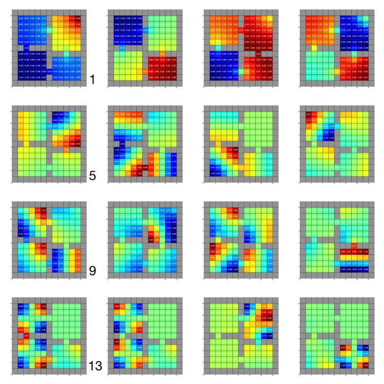
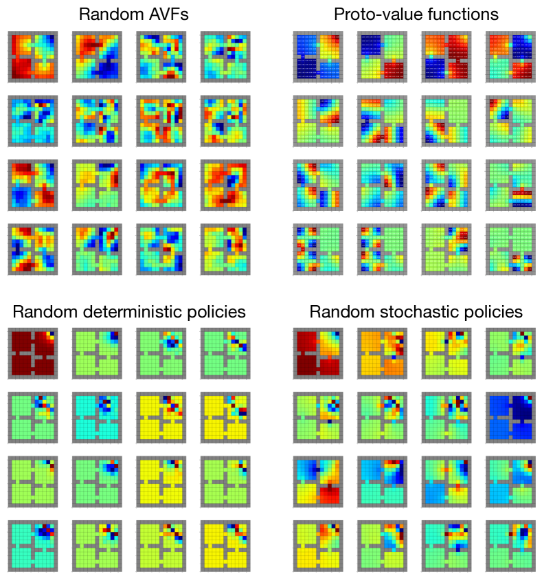
In Figure 10 we show the representations generated from this process, using different sets of value functions. For completeness, we consider:
-
•
1000 AVFs,
-
•
1000 random deterministic policies (RDPs),
-
•
1000 random stochastic policies (RSPs), and
-
•
The 104 rows of the successor matrix (corresponding to proto-value functions).
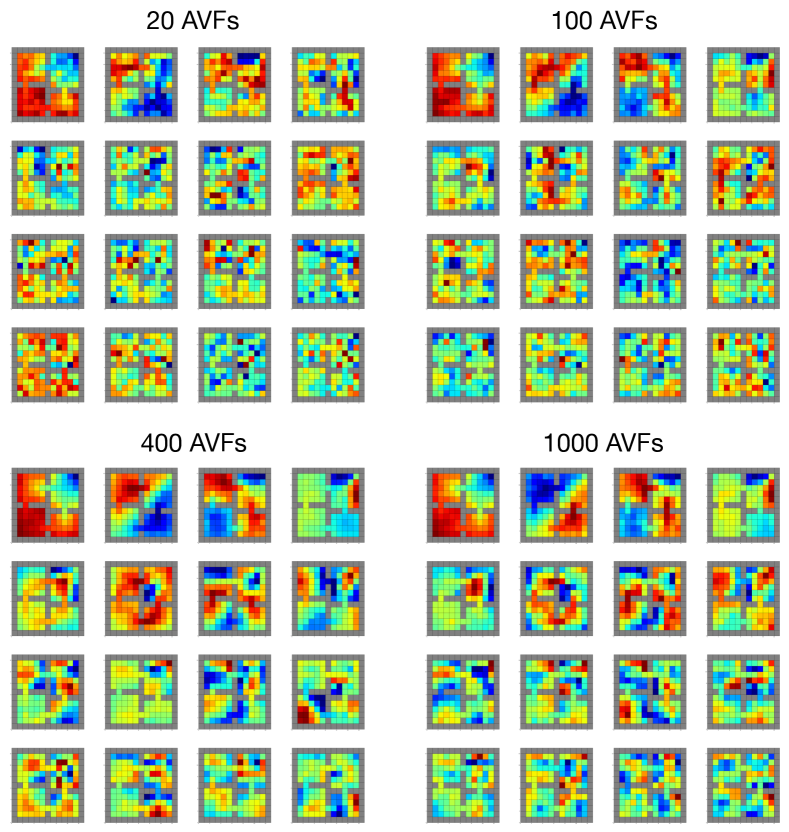
As with principal component analysis, the per-state feature activations are determined up to a signed scalar; we pick the vector which has more positive components than negative. In all but the PVF case, we sample a subset of the many possible value functions within a particular set. Figure 11 shows that the AVF approach is relatively robust to the sample size.
The AVFs are sampled using Algorithm 1, i.e. by sampling a random interest function and using policy gradient on a softmax policy to find the corresponding value function. The random policies were generated by randomly initializing the same softmax policy and using them as-is (RSPs) or multiplying the logits by 1e6 (RDPs).
