A Real-Time Optimal Eco-driving for Autonomous Vehicles Crossing Multiple Signalized Intersections*

Abstract

This paper develops an optimal acceleration/speed profile for a single autonomous vehicle crossing multiple signalized intersections without stopping in free flow mode. The design objective is to produce both time and energy efficient acceleration profiles of autonomous vehicles based on vehicle-to-infrastructure communication. Our design approach differs from most existing approaches based on numerical calculations: it begins with identifying the structure of the optimal acceleration profile and then showing that it is characterized by several parameters, which are used for design optimization. Therefore, the infinite dimensional optimal control problem is transformed into a finite dimensional parametric optimization problem, which enables a real-time online analytical solution. The simulation results show quantitatively the advantages of considering multiple intersections jointly rather than dealing with them individually. Based on mild assumptions, the optimal eco-driving algorithm is readily extended to include interfering traffic.

I Introduction

The alarming state of existing transportation systems has been well documented. For instance, in 2014, congestion caused vehicles in urban areas to spend 6.9 billion additional hours on the road at a cost of an extra 3.1 billion gallons of fuel, resulting in a total cost estimated at 160 billion [1]. From a control and optimization standpoint, the challenges stem from requirements for increased safety, increased efficiency in energy consumption, and lower congestion both in highway and urban traffic. Connected and automated vehicles (CAVs), commonly known as self-driving or autonomous vehicles, provide an intriguing opportunity for enabling users to better monitor transportation network conditions and to improve traffic flow. Their proliferation has rapidly grown, largely as a result of Vehicle-to-X (or V2X) technology [2] which refers to an intelligent transportation system where all vehicles and infrastructure components are interconnected with each other. Such connectivity provides precise knowledge of the traffic situation across the entire road network, which in turn helps optimize traffic flows, enhance safety, reduce congestion, and minimize emissions. Controlling a vehicle to improve energy consumption has been studied extensively, e.g., see [3, 4, 5, 6]. By utilizing road topography information, an energy-optimal control algorithm for heavy diesel trucks is developed in [5]. Based on Vehicle-to-Vehicle (V2V) communication, a minimum energy control strategy is investigated in car-following scenarios in [6]. Another important line of research focuses on coordinating vehicles at intersections to increase traffic flow while also reducing energy consumption. Depending on the control objectives, work in this area can be classified as dynamically controlling traffic signals [7] and as coordinating vehicles [8],[9],[10],[11]. More recently, an optimal control framework is proposed in [12] for CAVs to cross one or two adjacent intersections in an urban area. The state of art and current trends in the coordination of CAVs is provided in [13].

Our focus in this paper is on an optimal control approach for a single autonomous vehicle approaching multiple intersections in free flow mode in terms of energy consumption and taking advantage of traffic light information. The term “ECO-AND” (short for “Economical Arrival and Departure”) is often used in the literature to refer to this problem [14]. Its solution is made possible by vehicle-to-infrastructure (V2I) communication, which enables a vehicle to automatically receive signals from upcoming traffic lights before they appear in its visual range. For example, such a V2I communication system has been launched in Audi cars in Las Vegas by offering a traffic light timer on their dashboards: as the car approaches an intersection, a red traffic light symbol and a “time-to-go” countdown appear in the digital display and reads how long it will be before the traffic light ahead turns green [15]. Clearly, an autonomous vehicle can take advantage of such information in order to go beyond current “stop-and-go” to achieve “stop-free” driving. Along these lines, the problem of avoiding red traffic lights is investigated in [16, 17, 18, 19]. The purpose in [16] is to track a target speed profile, which is generated based on the feasibility of avoiding a sequence of red lights. The approach uses model predictive control based on a receding horizon. Avoiding red lights with probabilistic information at multiple intersections is considered in [17], where the time horizon is discretized and deterministic dynamic programming is utilized to numerically compute the optimal control input. The work in [18] devises the optimal speed profile given the feasible target time, which is within some green light interval. A velocity pruning algorithm is proposed in [19] to identify feasible green windows, and a velocity profile is calculated numerically in terms of energy consumption. Most existing work solves the eco-driving problem with traffic light constraints numerically, such as using dynamic programming [17, 20], and model predictive control [16]. To enable the real-time use of such eco-driving methods, it is desirable to have an on-line analytical solution.

From the above, it is clear that a need exists for developing new methods for eco-driving of autonomous vehicles with traffic light constraints. This paper aims to address this need by proposing an extension to our previous approach from a single signalized intersection [21, 22] to multiple intersections. We show explicitly that the optimal acceleration profile has a piecewise linear form, similar to the results in [21, 22], that includes all state equality and temporal inequality constraints involved. It follows from the theoretical analysis that the optimal acceleration profile can be parameterized by a piecewise linear function of time, which offers a real-time analytical solution to eco-driving of autonomous vehicles crossing multiple signalized intersections without stopping. We illustrate the effectiveness of the proposed optimal parametric approach through simulations and show that it yields better results compared with our previous eco-driving approach [21, 22] applied to each intersection individually. We also show that the optimal eco-driving algorithm can be adjusted to handle the case with interfering traffic under the assumption of the availability of some traffic information.

II Problem Formulation

The vehicle dynamics are modeled by a double integrator

$$\dot{x}\left(t\right) =v\left(t\right),$$ (1)

$$\dot{v}\left(t\right) =u\left(t\right),$$ (2)

where $x\left(t\right)$ is the travel distance of the vehicle relative to some origin on the road, which may include turns, $v\left(t\right)$ the velocity, and $u\left(t\right)$ the acceleration/deceleration. At $t_{0}$, the initial position and velocity are given by $x\left(t_{0}\right)=x_{0}$ and $v\left(t_{0}\right)=v_{0}$, respectively. On-road vehicles have to obey traffic rules, such as the minimum and maximum speed permitted $0<v_{\min}\leq v\left(t\right)\leq v_{\max}$. The physical constraints on acceleration and deceleration are determined by vehicle parameters $u_{\min}\leq u\left(t\right)\leq u_{\max}$, where $u_{\min}<0$ and $u_{\max}>0$ denote the maximum deceleration and acceleration, respectively.

Assume that there are $N$ intersections. Each intersection $i$ is equipped with a traffic light, which is dictated by the square wave $f_{i}\left(t\right)$ defined below

$$f_{i}\left(t\right)=\left\{\begin{array}[]{ll}1,&\text{when }kT_{i}\leq t\leq kT_{i}+D_{i}T_{i},\\ 0,&\text{when }kT_{i}+D_{i}T_{i}<t<kT_{i}+T_{i},\end{array}\right.$$

where $f_{i}\left(t\right)=1$ indicates that the traffic light is green, and $f_{i}\left(t\right)=0$ indicates that the traffic light is red. The parameter $0<D_{i}<1$ is the fraction of the time period $T_{i}$ during which the traffic light is green, and $k=0,1,\ldots,$ are non-negative integers. Assume that there is no offset among the signals. Our algorithm also supports dynamically actuated traffic signals if the time until green/red can be determined and communicated to the autonomous vehicle. Then we can re-solve the problem with the new timing information.

Let $\{t_{i}\}_{i=1}^{N}$ be a sequence of intersection crossing times with $t_{i+1}>t_{i}$, that is, $x\left(t_{i}\right)=\sum\nolimits_{j=1}^{i}l_{j}$, where $l_{j}$ is the length of road segment $j$. To ensure stop-free intersection crossing, $t_{i}$ must be within the green light interval, that is, $kT_{i}\leq t_{i}\leq kT_{i}+D_{i}T_{i}$ for some non-negative integer $k$.

Our objective is the eco-driving of autonomous vehicles crossing multiple intersections in terms of both time and energy efficiency. Therefore, our problem formulation is given below:

Problem 1

ECO-AND Problem

$$\min_{u\left(t\right)}\rho_{t}\left(t_{p}-t_{0}\right)+\rho_{u}\int_{t_{0}}^{t_{p}}u^{2}\left(t\right)dt$$

subject to

$$\left(\text{\ref{dd}}\right)\text{ and }\left(\text{\ref{vd}}\right)$$ (3)

$$x\left(t_{i}\right)=\sum\nolimits_{j=1}^{i}l_{j},\text{ }i=1,\ldots,N$$ (4)

$$v_{\min}\leq v\left(t\right)\leq v_{\max}$$ (5)

$$u_{\min}\leq u\left(t\right)\leq u_{\max}$$ (6)

$$k_{i}T_{i}\leq t_{i}\leq k_{i}T_{i}+D_{i}T_{i},\text{ }i=1,\ldots,N$$ (7)

for some non-negative integers $k_{i}$, where $\rho_{t}$ and $\rho_{u}$ are the weighting parameters, and $t_{p}=t_{N}$ is the time when the vehicle arrives at the last intersection.

Procedures for normalizing these two terms for the purpose of a well-defined optimization problem can be found in [21, 22] by properly determining weights $\rho_{t}$ and $\rho_{u}$. In Problem 1, the term $J^{t}=t_{p}-t_{0}$ is the travel time while $J^{u}=\int_{t_{0}}^{t_{p}}u^{2}\left(t\right)dt$ captures the energy consumption; see [23].

III Main Results

Before proceeding further, let us first introduce a lemma, which will be used frequently throughout the following analysis.

Lemma 1

Consider the vehicle’s dynamics (1) and (2) with initial conditions $x_{0}$ and $v_{0}$. If the acceleration profile of the vehicle has the form $u\left(t\right)=at+b$ during the time interval $\left[t_{0},t_{1}\right],$ where $a$ and $b$ are two constants, then

$$v\left(t_{1}\right)= v_{0}+b\left(t_{1}-t_{0}\right)+\frac{a}{2}\left(t_{1}^{2}-t_{0}^{2}\right)\text{,}$$

$$x\left(t_{1}\right)= x_{0}+v_{0}\left(t_{1}-t_{0}\right)+\frac{1}{2}b\left(t_{1}-t_{0}\right)^{2}$$

$$\quad+\frac{a}{6}\left(t_{1}^{3}+2t_{0}^{3}-3t_{0}^{2}t_{1}\right)\text{,}$$

$$J^{u}\left(t_{1}\right)= \frac{a^{2}}{3}\left(t_{1}^{3}-t_{0}^{3}\right)+ab\left(t_{1}^{2}-t_{0}^{2}\right)+b^{2}\left(t_{1}-t_{0}\right)\text{.}$$

The proof is obtained by using the kinematic equations of the vehicle (1) and (2) and the definition of $J_{u}$. Due to space constraints, the details are omitted.

Remark 1

We will show in Theorem 1 below that in fact the optimal acceleration profile for Problem 1 is of the form $u\left(t\right)=at+b$, which captures most acceleration profiles used in the literature and vehicle simulation software [24]. When $a=b=0$, the vehicle travels at a constant speed. When $a=0$, the acceleration profile becomes either constant acceleration ($b>0$) or constant deceleration ($b<0$). When $a\neq 0$, the resulting linear acceleration profile is also called “smooth jerk” [24].

In order not to overshadow the main idea, we consider the case of only two consecutive intersections here, where $t_{p}=t_{2}$. We will show how the proposed framework can include our previous result on a single intersection [21, 22] as a special case in Subsection IV-A and can be extended to the case of more than two intersections in Subsection IV-B.

The main challenge of extending the result from one intersection [21, 22] to multiple intersections lies in the interior-point constraints $x\left(t_{1}\right)=l_{1}$ and $kT_{1}\leq t_{1}\leq kT_{1}+D_{1}T_{1}$. Note that we have both a spatial equality constraint and a temporal inequality constraint. Other constraints, such as states, acceleration/deceleration, and terminal constraints, have been thoroughly studied in our previous work [21, 22]. The following theorem shows how the optimal acceleration profile is affected by the interior-point constraints.

Theorem 1

The optimal acceleration profile $u^{\ast}\left(t\right)$ of Problem 1 has the form

$$u^{\ast}\left(t\right)=a\left(t\right)t+b\left(t\right),$$

where $a\left(t\right)$ and $b\left(t\right)$ are piece-wise constant. In addition, $u^{\ast}\left(t\right)$ is continuous everywhere, and $u^{*}(t_{p}^{*})=0$.

Proof:

The interior-point constraints are dealt with by using the calculus of variations methodology borrowed from [25] with certain modifications. The Hamiltonian $H(v,u,\lambda)$ and Lagrangian $L(v,u,\lambda,\mu,\eta)$ are defined as

$$H\left(v,u,\lambda\right)=\rho_{t}+\rho_{u}u^{2}\left(t\right)+\lambda_{1}\left(t\right)v\left(t\right)+\lambda_{2}\left(t\right)u\left(t\right)$$

and

$$L\left(v,u,\lambda,\mu,\eta\right)= H\left(v,u,\lambda\right)+\eta_{1}\left(t\right)\left[v_{\min}-v\left(t\right)\right]$$

$$+\eta_{2}\left(t\right)\left[v\left(t\right)-v_{\max}\right]$$

$$+\mu_{1}\left(t\right)\left[u_{\min}-u\left(t\right)\right]$$

$$+\mu_{2}\left(t\right)\left[u\left(t\right)-u_{\max}\right]\text{,}$$

respectively, where $\lambda\left(t\right)=\left[\lambda_{1}\left(t\right)\text{ }\lambda_{2}\left(t\right)\right]^{T}$, $\mu\left(t\right)=\left[\mu_{1}\left(t\right)\text{ }\mu_{2}\left(t\right)\right]^{T}$, $\eta\left(t\right)=\left[\eta_{1}\left(t\right)\text{ }\eta_{2}\left(t\right)\right]^{T}$, and

$$\eta_{1}\left(t\right)\geq 0,\text{ }\eta_{2}\left(t\right)\geq 0,$$ (8)

$$\eta_{1}\left(t\right)\left[v_{\min}-v\left(t\right)\right]+\eta_{2}\left(t\right)\left[v\left(t\right)-v_{\max}\right]=0,$$ (9)

$$\mu_{1}\left(t\right)\geq 0,\text{ }\mu_{2}\left(t\right)\geq 0,$$ (10)

$$\mu_{1}\left(t\right)\left[u_{\min}-u\left(t\right)\right]+\mu_{2}\left(t\right)\left[u\left(t\right)-u_{\max}\right]=0.$$ (11)

According to Pontryagin’s minimum principle, the optimal control $u^{\ast}\left(t\right)$ must satisfy

$$u^{\ast}\left(t\right)=\arg\min_{u_{\min}\leq u\left(t\right)\leq u_{\max}}H\left(v^{\ast}\left(t\right),u\left(t\right),\lambda\left(t\right)\right),$$ (12)

which allows us to express $u^{\ast}\left(t\right)$ in terms of the co-state $\lambda\left(t\right),$ resulting in

$$u^{\ast}\left(t\right)=\left\{\begin{array}[]{ll}u_{\max}&\text{when }-\frac{\lambda_{2}\left(t\right)}{2\rho_{u}}\geq u_{\max}\\ -\frac{\lambda_{2}\left(t\right)}{2\rho_{u}}&\text{when }u_{\min}\leq-\frac{\lambda_{2}\left(t\right)}{2\rho_{u}}\leq u_{\max}\\ u_{\min}&\text{when }-\frac{\lambda_{2}\left(t\right)}{2\rho_{u}}\leq u_{\min}\end{array}\right.$$ (13)

For simplicity, we write $L(t)$, $H(t)$, $J(t)$ and $N(t)$ without the arguments of states, co-states, and multipliers in the rest of the paper. Adjoin the system differential equations (1) and (2) to $L\left(t\right)$ with multiplier function $\lambda\left(t\right)$:

$$J\left(t\right)=N\left(t_{1},t_{p}\right)+\int_{t_{0}}^{t_{p}}\left[L\left(t\right)-\lambda_{1}\left(t\right)\dot{x}\left(t\right)-\lambda_{2}\left(t\right)\dot{v}\left(t\right)\right]dt,$$

where $t_{1}$ is the first intersection crossing time, and

$$N\left(t_{1},t_{p}\right)=\nu x\left(t_{p}\right)+\pi\left(x\left(t_{1}\right)-l\right)+\upsilon_{1}\left(k_{1}T_{1}-t_{1}\right)$$

$$\qquad\qquad+\upsilon_{2}\left(t_{1}-k_{1}T_{1}-D_{1}T_{1}\right),$$

$$\upsilon_{1}\geq 0,\quad\upsilon_{2}\geq 0,$$

$$\upsilon_{1}\left(k_{1}T_{1}-t_{1}\right)+\upsilon_{2}\left(t_{1}-k_{1}T_{1}-D_{1}T_{1}\right)=0.$$

The first variation of the augmented performance index is

$$\delta J\left(t\right)= \delta N\left(t_{1},t_{p}\right)$$

$$+\delta\int_{t_{0}}^{t_{p}}\left[L\left(t\right)-\lambda_{1}\left(t\right)\dot{x}\left(t\right)-\lambda_{2}\left(t\right)\dot{v}\left(t\right)\right]dt\text{.}$$

Split the integral into two parts:

$$\delta J\left(t\right) = \nu\delta x\left(t\right)|_{t=t_{p}}+\left(\upsilon_{2}-\upsilon_{1}\right)dt_{1}+\pi dx\left(t_{1}\right)$$

$$+\left[L\left(t\right)-\lambda_{1}\left(t\right)\dot{x}\left(t\right)-\lambda_{2}\left(t\right)\dot{v}\left(t\right)\right]|_{t=t_{1}^{-}}dt_{1}$$

$$-\left[L\left(t\right)-\lambda_{1}\left(t\right)\dot{x}\left(t\right)-\lambda_{2}\left(t\right)\dot{v}\left(t\right)\right]|_{t=t_{1}^{+}}dt_{1}$$

$$-\lambda_{1}\left(t\right)\delta x\left(t\right)|_{t_{0}}^{t_{1}^{-}}-\lambda_{1}\left(t\right)\delta x\left(t\right)|_{t_{1}^{+}}^{t_{p}}$$

$$-\lambda_{2}\left(t\right)\delta v\left(t\right)|_{t_{0}}^{t_{1}^{-}}-\lambda_{2}\left(t\right)\delta v\left(t\right)|_{t_{1}^{+}}^{t_{p}}$$

$$+\int_{t_{0}}^{t_{p}}\left[\dot{\lambda}_{2}\left(t\right)+\frac{\partial L\left(t\right)}{\partial v\left(t\right)}\right]\delta v\left(t\right)dt$$

$$+\int_{t_{0}}^{t_{p}}\left\{\dot{\lambda}_{1}\left(t\right)\delta x\left(t\right)+\frac{\partial L\left(t\right)}{\partial u\left(t\right)}\delta u\left(t\right)\right\}dt,$$

where we let $t_{1}^{-}$ signify just before $t_{1}$ and $t_{1}^{+}$ signify just after $t_{1}$. We now make use of the relationships

$$dx\left(t_{1}\right)=\left\{\begin{array}[]{c}\delta x\left(t_{1}^{-}\right)+\dot{x}\left(t_{1}^{-}\right)dt_{1},\\ \delta x\left(t_{1}^{+}\right)+\dot{x}\left(t_{1}^{+}\right)dt_{1},\end{array}\right.$$

and the relationships of $v\left(t\right)$ can be derived similarly. Using the above relationships to eliminate $\delta x\left(t_{1}^{-}\right)$ and $\delta x\left(t_{1}^{+}\right)$, and regrouping terms, yields

$$\delta J\left(t\right)= \left[v-\lambda_{1}\left(t\right)\right]\delta x\left(t\right)|_{t=t_{p}}-\lambda_{2}\left(t\right)\delta v\left(t\right)|_{t=t_{p}}$$

$$+\lambda_{1}\left(t\right)\delta x\left(t\right)|_{t=t_{0}}+\lambda_{2}\left(t\right)\delta v\left(t\right)|_{t=t_{0}}$$

$$+\left[L\left(t_{1}^{-}\right)-L\left(t_{1}^{+}\right)+\upsilon_{2}-\upsilon_{1}\right]dt_{1}$$ (14)

$$+\left[\lambda_{1}\left(t_{1}^{+}\right)-\lambda_{1}\left(t_{1}^{-}\right)+\pi\right]dx\left(t_{1}\right)$$

$$+\left[\lambda_{2}\left(t_{1}^{+}\right)-\lambda_{2}\left(t_{1}^{-}\right)\right]dv\left(t_{1}\right)$$

Since we have no constraint on $v\left(t\right)$ at $t=t_{1}$, it follows that $\lambda_{2}\left(t_{1}^{+}\right)=\lambda_{2}\left(t_{1}^{-}\right)$, that is to say, there are no discontinuities in $\lambda_{2}\left(t\right)$ at $t=t_{1}$. Therefore, $u^{\ast}\left(t\right)$ is continuous everywhere based on (12) and Theorem 1 in [21, 22]. To make the term $\lambda_{2}(t_{p})\delta v(t_{p})$ in (14) vanish, we must have $\lambda_{2}(t_{p})=0$ since there are no constraints on $v(t)$ at $t=t_{p}$. From the optimality condition (13), we have $u^{*}(t_{p}^{*})=0$.

For the co-state $\lambda_{1}\left(t\right),$ we have

$$\dot{\lambda}_{1}\left(t\right)=-\frac{\partial L^{\ast}\left(t\right)}{\partial x}=0.$$

However, since $dx\left(t_{1}\right)=0,$ $\lambda_{1}\left(t\right)$ may or may not have jumps at $t=t_{1}$. Therefore, $\lambda_{1}\left(t\right)$ can be written as

$$\lambda_{1}\left(t\right)=\left\{\begin{array}[]{cc}\lambda_{1}^{-}&\text{for }t_{0}\leq t\leq t_{1},\\ \lambda_{1}^{+}&\text{for }t_{1}<t\leq t_{p}\text{.}\end{array}\right.$$ (15)

For the co-state $\lambda_{2}\left(t\right),$ we have

$$\dot{\lambda}_{2}\left(t\right)=-\frac{\partial L^{\ast}\left(t\right)}{\partial v}=-\lambda_{1}\left(t\right)+\eta_{1}\left(t\right)-\eta_{2}\left(t\right)\text{.}$$ (16)

Depending on the value of $v\left(t\right),$ we have different cases:

Case I: $v_{\min}<v\left(t\right)<v_{\max}$. In this case, $\eta_{1}\left(t\right)=\eta_{2}\left(t\right)=0$. Therefore, $\lambda_{2}\left(t\right)$ linearly increases or decreases according to (15) and (16), and so does $u^{\ast}\left(t\right)$ based on (13).

Case II: $v\left(\tau\right)=v_{\min}$. In this case, we have $u^{\ast}\left(t\right)\geq 0$ over some interval $[\tau,\tau+\alpha]$. When $u^{\ast}\left(t\right)=0$ over the interval $[\tau,\tau+\alpha]$, we must have $\lambda_{2}(t)=\dot{\lambda}_{2}(t)=0$, that is, $\eta_{1}\left(t\right)=\lambda_{1}\left(t\right)$ from (16) and the fact that $\eta_{2}(t)=0$ based on (9). When $u^{\ast}\left(\tau^{+}\right)>0,$ $v\left(\tau^{+}\right)>v_{\min}$. Then, it becomes Case I.

Case III: $v\left(\tau\right)=v_{\max}$. In this case, we have $u^{\ast}\left(t\right)\leq 0$ over some interval $[\tau,\tau+\alpha]$. When $u^{\ast}\left(t\right)=0$ over the interval $[\tau,\tau+\alpha]$, we have $\lambda_{2}(t)=\dot{\lambda}_{2}(t)=0$, that is, $\eta_{2}\left(t\right)+\lambda_{1}\left(t\right)=0$ from (16) and the fact that $\eta_{1}(t)=0$ based on (9). When $u^{\ast}\left(\tau^{+}\right)<0$, $v\left(\tau^{+}\right)<v_{\max}$. Then, it becomes Case I.

Regardless of which of these three cases applies, the optimal control $u^{\ast}\left(t\right)$ always has a linear form. ∎

Remark 2

Assume that at $t_{1}$ all the states and acceleration/deceleration constraints are relaxed. Then $L\left(t\right)$ is the same as $H\left(t\right)$. To cause the coefficient of $dt_{1}$ to vanish, the condition $L\left(t_{1}^{-}\right)-L\left(t_{1}^{+}\right)+\upsilon_{2}-\upsilon_{1}=0$ has to be satisfied. If $kT_{1}<t_{1}<kT_{1}+D_{1}T_{1}$, then $\upsilon_{2}=\upsilon_{1}=0$. Therefore, there are no jumps in $L\left(t\right)$ and $H\left(t\right)$ at $t_{1}$. In other words, the co-state $\lambda_{1}$ has no jumps in this case. However, when $t_{1}=kT_{1}$ or $t_{1}=kT_{1}+D_{1}T_{1}$, there may be jumps in $L\left(t\right)$ and $H\left(t\right)$ at $t_{1}$. Then $\lambda_{1}$ switches from one value to another as shown in (15).

Based on Theorem 1, we know that the optimal acceleration profile has the form $u^{\ast}\left(t\right)=a\left(t\right)t+b\left(t\right)$, where $a\left(t\right)$ and $b\left(t\right)$ are piece-wise constant.  For example, we have $a\left(t\right)=0,\quad b\left(t\right)=u_{\max}$ for $u^{\ast}\left(t\right)=u_{\max}$, and $a\left(t\right)=0,\quad b\left(t\right)=u_{\min}$ for $u^{\ast}\left(t\right)=u_{\min}$. For the case that $u\left(t\right)=0$, we could set $a\left(t\right)=b\left(t\right)=0$. Most of the time, $a\left(t\right)=a$ and $b\left(t\right)=b$ are just constants. In addition, there are only a few time instants when $a\left(t\right)$ and $b\left(t\right)$ switch from a constant to another. Such instants include the time when the maximum acceleration starts to decrease, the maximum deceleration starts to increase, the vehicle reaches the maximum or the minimum allowed speed limits, or at the first intersection crossing time $t_{1}$. Therefore, we could parameterize the optimal acceleration profile by a sequence of linear functions of time.

IV Parametric Optimization

Based on the analysis of the last section, the optimal acceleration profile can be parameterized by a sequence of linear functions of time, such as the one shown in Fig. 1. Now let us split the analysis into two parts: $\left[t_{0},t_{1}\right]$ and $\left[t_{1},t_{2}\right]$, where $t_{1}$ is the first intersection crossing time. The optimal acceleration profile at most has four switches at $\tau_{1},\tau_{3},\tau_{5},\tau_{6}$ as shown in Fig. 1. The acceleration profile shown in Fig. 1 is the most complicated acceleration profile possible, starting with the maximum acceleration, which can be obtained based on the optimality condition (13) and the following facts:

• $u^{\ast}\left(t_{2}^{*}\right)=0,$ which can be seen from Theorem 1.

• Whenever $v\left(t\right)=v_{\min}$ or $v_{\max}$, $u^{\ast}\left(t\right)=0$.

• $u^{\ast}\left(t\right)$ is continuous without jumps.

• Only at $t_{1},$ $\dot{\lambda}_{2}\left(t\right)$ may change sign according to (16).

Figure 1: Optimal acceleration profile for two intersections

A similar optimal acceleration profile can be drawn when it starts with the maximum deceleration. The second fact above corresponds to the interval $[\tau_{6},\tau_{7}]$ in Fig. 1, in which $v(t)=v_{\min}$ for $t\in[\tau_{6},\tau_{7}]$. The fourth fact above can be visualized in Fig. 1 as well. Before $\tau_{4}$, the acceleration decreases monotonically; and after $\tau_{4}$ it increases monotonically. Even though there are five linear functions in Fig. 1, seven linear functions are needed to parameterize the acceleration profile. Over the interval $[\tau_{1},\tau_{3}]$ in Fig. 1, there is only one linear function. In order to guarantee that the acceleration profile during each interval contains either acceleration or deceleration but not both, which is ensured by the constraint (18) below, we consider that there is a switch at $\tau_{2}$ between acceleration and deceleration. Therefore, two linear functions are used to parameterize the optimal acceleration profile. By doing so, the speed either increases or decreases during each interval. Therefore, the constraint (17) below ensures that the speed is within the minimum and maximum bounds all the time.

We can thus parameterize the optimal acceleration profile as follows:

$$u^{\ast}\left(t\right)=\left\{\begin{array}[]{cc}a_{1}t+b_{1}&\text{for }t\in\left[\tau_{0},\tau_{1}\right]\\ a_{2}t+b_{2}&\text{for }t\in\left[\tau_{1},\tau_{2}\right]\\ a_{3}t+b_{3}&\text{for }t\in\left[\tau_{2},\tau_{3}\right]\\ a_{4}t+b_{4}&\text{for }t\in\left[\tau_{3},\tau_{4}\right]\\ a_{5}t+b_{5}&\text{for }t\in\left[\tau_{4},\tau_{5}\right]\\ a_{6}t+b_{6}&\text{for }t\in\left[\tau_{5},\tau_{6}\right]\\ a_{7}t+b_{7}&\text{for }t\in\left[\tau_{6},\tau_{7}\right]\end{array}\right.$$

where $\tau_{0}=t_{0},$ $\tau_{4}=t_{1}$, and $\tau_{7}=t_{2}$.

Remark 3

The optimal acceleration profile is overapproximated by the triplets $(a_{i},b_{i},\tau_{i})$, $i=1,2,\ldots,7$, 21 variables in total. The number of variables can be reduced when the properties of $u^{*}(t)$ are considered. The advantage of the parametric form of the optimal controller is that it simplifies the complicated analysis through a computationally efficient scheme suitable for real-time implementation. Also note that vehicles may experience both acceleration and deceleration during a single road segment, which is different from the optimal acceleration profile for a single intersection [21, 22].

We have now shown that Problem 1 is equivalent to this parametric optimization problem:

Problem 2

ECO-AND problem

$$\min\rho_{t}\tau_{7}+\rho_{u}\sum_{i=1}^{7}J^{u}_{i}$$

subject to

$$v_{\min}\leq v\left(\tau_{i}\right)\leq v_{\max},$$ (17)

$$\left(a_{i}\tau_{i}+b_{i}\right)\left(a_{i}\tau_{i-1}+b_{i}\right)\geq 0,$$ (18)

$$u_{\min}\leq a_{i}\tau_{i}+b_{i}\leq u_{\max},$$ (19)

$$u_{\min}\leq a_{i}\tau_{i-1}+b_{i}\leq u_{\max},$$ (20)

$$\tau_{i-1}\leq\tau_{i},$$ (21)

$$i=1,\ldots,7,$$

$$k_{1}T_{1}\leq\tau_{4}\leq k_{1}T_{1}+D_{1}T_{1},$$ (22)

$$x\left(\tau_{4}\right)=l_{1}$$ (23)

$$k_{2}T_{2}\leq\tau_{7}\leq k_{2}T_{2}+D_{2}T_{2},$$ (24)

$$x\left(\tau_{7}\right)=l_{1}+l_{2}$$ (25)

where $J^{u}_{i}$ is the energy cost during the interval $[\tau_{i-1},\tau_{i}]$, which can be obtained as

$$J^{u}_{i}=\frac{a_{i}^{2}}{3}\left(\tau_{i}^{3}-\tau_{i-1}^{3}\right)+a_{i}b_{i}\left(\tau_{i}^{2}-\tau_{i-1}^{2}\right)+b_{i}^{2}\left(\tau_{i}-\tau_{i-1}\right)$$

from Lemma 1,

$$v\left(\tau_{i}\right)=v\left(\tau_{i-1}\right)+b_{i}\left(\tau_{i}-\tau_{i-1}\right)+\frac{a_{i}}{2}\left(\tau_{i}^{2}-\tau_{i-1}^{2}\right)$$

and

$$x\left(\tau_{i}\right) = x\left(\tau_{i-1}\right)+v\left(\tau_{i-1}\right)\left(\tau_{i}-\tau_{i-1}\right)$$

$$+\frac{b_{i}}{2}\left(\tau_{i}-\tau_{i-1}\right)^{2}+\frac{a_{i}}{6}\left(\tau_{i}^{3}+2\tau_{i-1}^{3}-3\tau_{i-1}^{2}\tau_{i}\right).$$

Remark 4

Problem 2 is equivalent to Problem 1, where the continuous velocity constraint (5) is ensured by (17) and (18). The continuous acceleration constraint (6) is ensured by (19) and (20). The constraint (21) is needed to ensure the right order of the intersection crossing times of the autonomous vehicle driven by the optimal acceleration profile.

Remark 5

The parametric optimization framework is very general so that it can be used to solve many different eco-driving problems. By taking into consideration the driving comfort, we can just add the constraints $\left|a_{i}\right|\leq a_{J}$, where $a_{i}$ corresponds to the jerk profile, and $a_{J}$ is the limit of jerk tolerance [14]. The parametric optimization framework can also easily incorporate an initial acceleration condition, interior and terminal velocity/acceleration constraints by adding additional equality or inequality constraints.

In the following, we will show how this optimal parametric framework includes our previous result [21, 22] as a special case, and how to extend the framework to more than two intersections.

IV-A Single Intersection

Based on our analysis for a single intersection [21, 22], the optimal acceleration profile can be parameterized as

$$u^{\ast}\left(t\right)=\left\{\begin{array}[]{cc}a_{1}t+b_{1}&\text{for }t\in\left[\tau_{0},\tau_{1}\right]\\ a_{2}t+b_{2}&\text{for }t\in\left[\tau_{1},\tau_{2}\right]\\ a_{3}t+b_{3}&\text{for }t\in\left[\tau_{2},\tau_{3}\right]\end{array}\right.$$

where $\tau_{0}=t_{0}$, and $\tau_{3}=t_{1}$. The optimal parameters $\left(a_{i},b_{i},\tau_{i}\right)$ for $i=1,2,3$ can be obtained by solving the following optimization problem:

Problem 3

ECO-AND problem

$$\min\rho_{t}\tau_{3}+\rho_{u}\sum_{i=1}^{3}J^{u}_{i}$$

subject to

$$v_{\min}\leq v\left(\tau_{3}\right)\leq v_{\max}$$ (26)

$$u_{\min}\leq a_{1}\tau_{0}+b_{1}\leq u_{\max}$$ (27)

$$\tau_{i-1}\leq\tau_{i},\quad i=1,\ldots,3$$ (28)

$$kT\leq\tau_{3}\leq kT+DT$$ (29)

$$x\left(\tau_{3}\right)=l,$$ (30)

where $J^{u}_{i}$ is the energy cost during the interval $\left[\tau_{i-1},\tau_{i}\right],$ which can be obtained as

$$J^{u}_{i}=\frac{a_{i}^{2}}{3}\left(\tau_{i}^{3}-\tau_{i-1}^{3}\right)+a_{i}b_{i}\left(\tau_{i}^{2}-\tau_{i-1}^{2}\right)+b_{i}^{2}\left(\tau_{i}-\tau_{i-1}\right)$$

according to Lemma 1, and

$$x\left(\tau_{i}\right) = x\left(\tau_{i-1}\right)+v\left(\tau_{i-1}\right)\left(\tau_{i}-\tau_{i-1}\right)$$

$$+\frac{b_{i}}{2}\left(\tau_{i}-\tau_{i-1}\right)^{2}+\frac{a_{i}}{6}\left(\tau_{i}^{3}+2\tau_{i-1}^{3}-3\tau_{i-1}^{2}\tau_{i}\right)$$

$$v\left(\tau_{i}\right) = v\left(\tau_{i-1}\right)+b_{i}\left(\tau_{i}-\tau_{i-1}\right)+\frac{a_{i}}{2}\left(\tau_{i}^{2}-\tau_{i-1}^{2}\right).$$

Note that we do not include the constraint (18) here since we have established the result in [21, 22] that the optimal acceleration profile contains either acceleration or deceleration, but not both. Therefore, the terminal velocity constraint (26) can replace the velocity constraint (17). Also based on the analysis in [21, 22], the initial acceleration constraint (27) is sufficient instead of using (19) and (20).

IV-B Multiple Intersections

The optimal parametric framework for two intersections can be easily extended to the case of more than two intersections. We can use three triplets $\left(a_{i},b_{i},\tau_{i}\right)$ to parameterize the optimal acceleration profile for a single intersection. For double intersections, seven triplets $\left(a_{i},b_{i},\tau_{i}\right)$ are enough to parameterize the optimal acceleration profile. It can be obtained by mathematical induction that $4\left(N-1\right)+3$ triplets of the form $\left(a_{i},b_{i},\tau_{i}\right)$ are enough to characterize the optimal acceleration profile for $N$ intersections, where the proof will be shown in a later version of this paper.

Therefore, for $N$ intersections, the ECO-AND problem can be solved by the following optimization problem:

Problem 4

ECO-AND problem

$$\min\rho_{t}\tau_{4(N-1)+3}+\rho_{u}\sum_{i=1}^{4\left(N-1\right)+3}J^{u}_{i}$$

subject to

$$v_{\min}\leq v\left(\tau_{i}\right)\leq v_{\max}$$

$$\left(a_{i}\tau_{i}+b_{i}\right)\left(a_{i}\tau_{i-1}+b_{i}\right)\geq 0$$

$$u_{\min}\leq a_{i}\tau_{i}+b_{i}\leq u_{\max},$$

$$u_{\min}\leq a_{i}\tau_{i-1}+b_{i}\leq u_{\max},$$

$$\tau_{i-1}\leq\tau_{i},$$

$$i=1,2,\ldots,4\left(N-1\right)+3,$$

$$k_{\left\lceil\frac{j}{4}\right\rceil}T_{\left\lceil\frac{j}{4}\right\rceil}\leq\tau_{j}\leq k_{\left\lceil\frac{j}{4}\right\rceil}T_{\left\lceil\frac{j}{4}\right\rceil}+D_{\left\lceil\frac{j}{4}\right\rceil}T_{\left\lceil\frac{j}{4}\right\rceil},$$

$$x\left(\tau_{j}\right)=\sum\nolimits_{i=1}^{\left\lceil\frac{j}{4}\right\rceil}l_{i}$$

$$j=4,8,\ldots,4\left(N-1\right),4\left(N-1\right)+3,$$

where $J^{u}_{i}$ is the energy cost during the interval $\left[\tau_{i-1},\tau_{i}\right]$, which can be obtained as

$$J^{u}_{i}=\frac{a_{i}^{2}}{3}\left(\tau_{i}^{3}-\tau_{i-1}^{3}\right)+a_{i}b_{i}\left(\tau_{i}^{2}-\tau_{i-1}^{2}\right)+b_{i}^{2}\left(\tau_{i}-\tau_{i-1}\right)$$

from Lemma 1, $\left\lceil x\right\rceil$ is the smallest integer greater than or equal to $x,$

$$v\left(\tau_{i}\right)=v\left(\tau_{i-1}\right)+b_{i}\left(\tau_{i}-\tau_{i-1}\right)+\frac{a_{i}}{2}\left(\tau_{i}^{2}-\tau_{i-1}^{2}\right)$$

and

$$x\left(\tau_{i}\right) = \sum_{j=1}^{i-1}l_{j}+v\left(\tau_{i-1}\right)\left(\tau_{i}-\tau_{i-1}\right)$$

$$+\frac{b_{i}}{2}\left(\tau_{i}-\tau_{i-1}\right)^{2}+\frac{a_{i}}{6}\left(\tau_{i}^{3}+2\tau_{i-1}^{3}-3\tau_{i-1}^{2}\tau_{i}\right).$$

V EXTENSION TO CASES WITH INTERFERING TRAFFIC

In the above results, we assume that a single vehicle operates in free flow mode. However, the proposed method can be easily extended to traffic conditions where other road users may affect the movement of the autonomous vehicle. Therefore, a safety constraint has to be enforced at all times, that is,

$$x_{h}\left(t\right)-x\left(t\right)\geq\alpha v\left(t\right)+\beta$$ (31)

where $x_{h}$ is the position of the preceding vehicle, $\alpha$ and $\beta$ are two scalars representing dynamic and static gaps, respectively [26]. The following assumptions are made:

• On the road, the future speed and acceleration profiles of the preceding vehicle can be estimated accurately enough by the autonomous vehicle.

• At the intersection, the queue information and stopped vehicle lengths are also available to the autonomous vehicle.

When the proposed approach without considering interfering traffic is applied, the safety constraint in (31) may be violated. The first case is that the preceding vehicle will cross the intersection at some $t\in[kT_{i},kT_{i}+D_{i}T_{i}]$ while the autonomous vehicle will not. In this case, the autonomous vehicle becomes the leading vehicle on the road, and the intersection crossing time is set as the beginning of the next green light interval $t_{i}=kT_{i+1}$ for some positive integer $k$. The safety constraint may not be violated since the preceding vehicle will accelerate or cruise through the intersection while the autonomous vehicle will decelerate to approach the intersection in the next green light interval. The second case is that both the preceding vehicle and the autonomous vehicle will cross the intersection at the same green light interval. In this case, we can simply decrease the maximum speed to $\theta v_{\max}$ with $0<\theta<1$ so that the safety constraint is satisfied at all times. The third case is that the preceding vehicle stopped before the intersection. In this case, the autonomous vehicle will cross the intersection after the preceding vehicle with a certain time gap $\sigma$ when the traffic signal turns to green so that the safety constraint is not violated, that is, $t_{i}=kT_{i}+\sigma$.

VI SIMULATION EXAMPLES

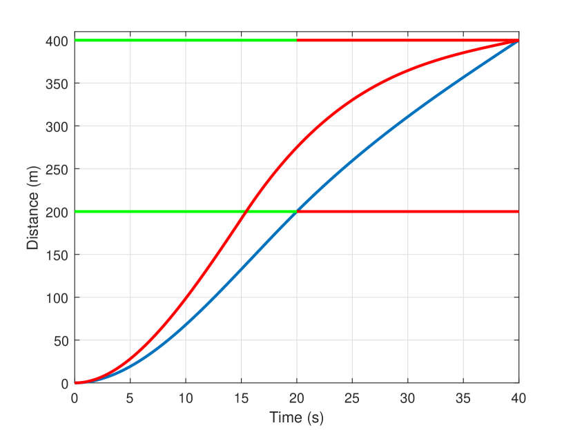
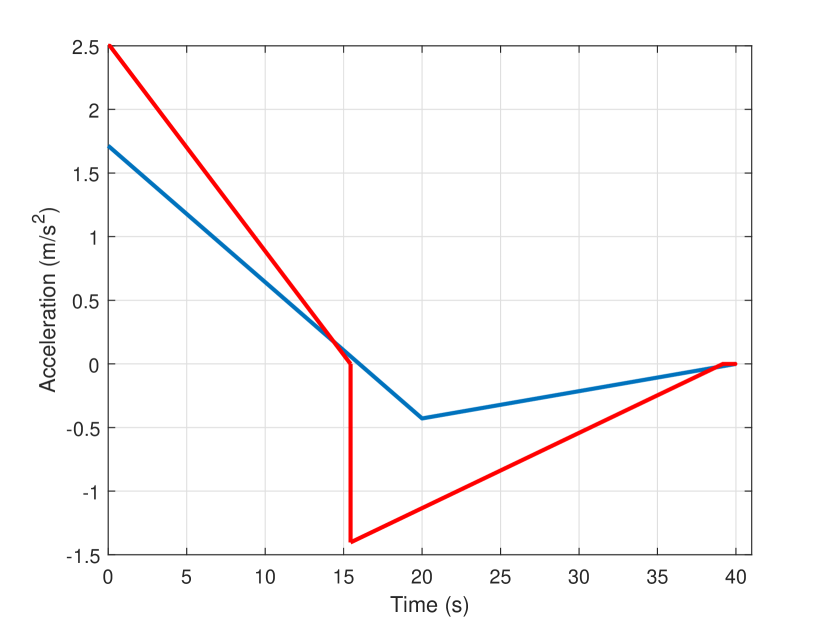
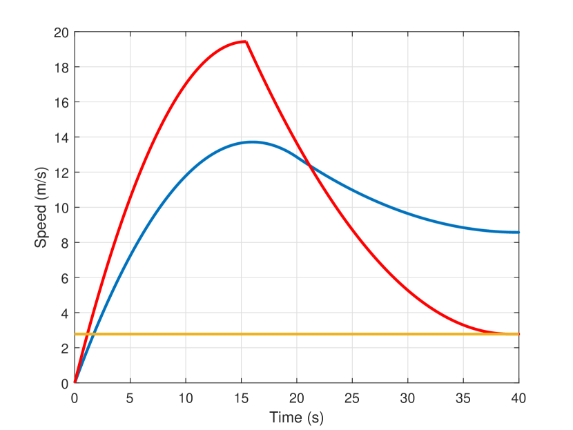
We evaluate the proposed solution by testing the following scenario with two intersections in MATLAB. The length for each road segment is 200 meters. Each intersection is equipped with a traffic light. Two phases were set up for each signal. The total cycle is 40 seconds, where the green time is set to 20 seconds. The speed limits are set as $v_{m}=2.78$ $m/s,$ and $v_{M}=20$ $m/s$. The maximum acceleration and deceleration are $u_{M}=2.5$ $m/s^{2}$ and $u_{m}=-2.9$ $m/s^{2}$. We assume that the vehicle starts with $v_{0}=0$. We use our previous approach for a single intersection [21, 22] as the baseline scenario, which solves the eco-driving problem for each road segment individually, and compare the proposed solution and the baseline scenario. Table I shows the performance by using our previous approach [21, 22] and the optimal parametric approach. Even though our previous approach [21, 22] calculates the optimal performance for each road segment, it is not the optimal solution for the combined two segments as a whole. Overall, the optimal multi-intersection parametric approach outperforms [21, 22] by $10.29\%$. Figures 2-4 show the acceleration, speed, and distance profiles for both the optimal multi-intersection parametric approach (blue curve) and [21, 22] (red curve). The optimal multi-intersection parametric approach verifies the properties of the optimal acceleration profile, that is, continuity and $u^{*}(t_{p}^{*})=0$ even though such constraints are not enforced in Problem 2. In addition, the speed profile of the optimal multi-intersection parametric approach is smoother than that of [21, 22] as seen from Fig. 3. We can see from Fig. 4 that the intersection crossing times of both approaches are within the green light interval. The travel time is 40 seconds for both approaches, which is determined by the second traffic light. However, their first intersection crossing times are different.

Figure 2: Acceleration profile of different methods: blue is the optimal multi-intersection parametric approach and red is the controller from [21, 22].

Figure 3: Speed profile of different methods: blue is the optimal multi-intersection parametric approach and red is the controller from [21, 22].

Figure 4: Distance profile of different methods: blue is the optimal multi-intersection parametric approach and red is the controller from [21, 22].

TABLE I: Performance Comparison

Method	Performance
	$J_{1}$	$J_{2}$	$J$
[21, 22]	$0.1366$	$0.1793$	$0.3159$
Optimal Parametric Approach	$0.1494$	$0.1340$	$0.2834$
Improvement	$-9.67\%$	$25.26\%$	$10.29\%$

VI-A Example with Interfering Traffic

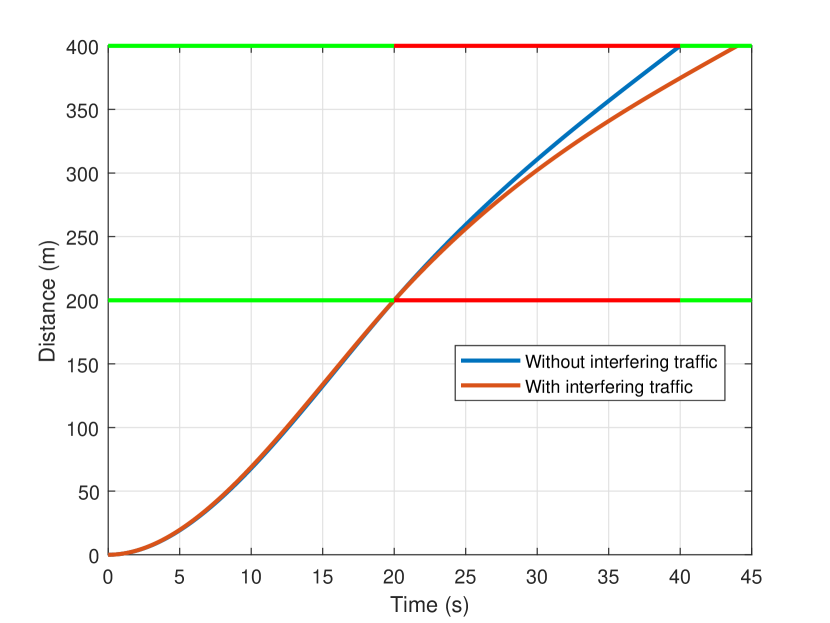
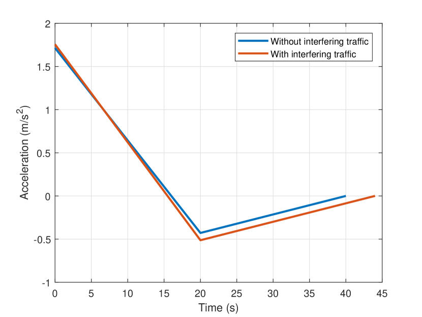
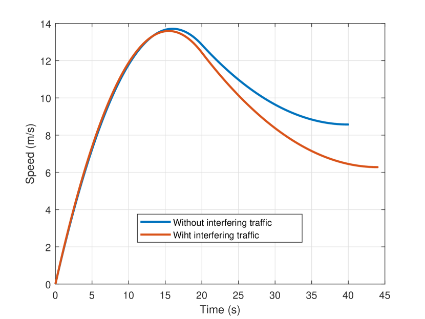
In the following, we consider a scenario where the autonomous vehicle will not be obstructed on the road but there is a vehicle which will stop before the second intersection. We assume that such information is available to the autonomous vehicle at time $t_{0}$. It is infeasible for the autonomous vehicle to cross the second intersection at 40 seconds as before. We assume that the feasible intersection crossing time is $t\in[44,60]$, where the four seconds include driver’s reaction time, headway time, and time for the stopped vehicle to clear the intersection. Figures 5-7 depict the acceleration profiles, speed profiles, and distance profiles, respectively, for both the cases with and without interfering traffic. It can be seen from the figures that the first intersection crossing times are the same for both cases. However, when there is interfering traffic, the autonomous vehicle has to start with a higher acceleration and decelerate more before the first intersection compared with the case without interfering traffic.

Figure 5: Acceleration profiles of the optimal solution with and without interfering traffic.

Figure 6: Speed profiles of the optimal solution with and without interfering traffic.

Figure 7: Distance profiles of the optimal solution with and without interfering traffic.

Here we do not compare the results with those of human-driven vehicles due to space constraints. Such a comparison was done in our previous work for a single intersection [21, 22], where 2%-10% performance improvement was shown in terms of travel time and fuel consumption.

VII Conclusions

In this paper, we solve an eco-driving problem of autonomous vehicles crossing multiple intersections without stopping. Spatial equality constraints and temporal inequality constraints are used to capture the traffic light constraints. Inspired by our previous work on a single intersection, the optimal acceleration profile is proved to have a piece-wise linear parametric structure. We illustrate the effectiveness of the proposed parametric approach through simulation examples. The results show that the performance is significantly improved by using the proposed optimal parametric approach compared with our previous approach which is optimal for each individual intersection decoupled from the other. We also show that the optimal eco-driving algorithm is capable of dealing with interfering traffic.

References

• [1] D. Schrank, B. Eisele, T. Lomax, and J. Bak, “2015 urban mobility scorecard,” Texas A&M Transportation Institute and INRIX, Tech. Rep., 2015.
• [2] L. Li, D. Wen, and D. Yao, “A survey of traffic control with vehicular communications,” IEEE Trans. Intell. Transport. Syst., vol. 15, no. 1, pp. 425–432, 2014.
• [3] E. G. Gilbert, “Vehicle cruise: Improved fuel economy by periodic control,” Automatica, vol. 12, no. 2, pp. 159 – 166, 1976.
• [4] J. Hooker, “Optimal driving for single-vehicle fuel economy,” Transportation Research Part A: General, vol. 22, no. 3, pp. 183 – 201, 1988.
• [5] E. Hellstrom, J. Aslund, and L. Nielsen, “Design of an efficient algorithm for fuel-optimal look-ahead control,” Control Engineering Practice, vol. 18, no. 11, pp. 1318 – 1327, 2010.
• [6] S. E. Li, H. Peng, K. Li, and J. Wang, “Minimum fuel control strategy in automated car-following scenarios,” IEEE Transactions on Vehicular Technology, vol. 61, no. 3, pp. 998–1007, 2012.
• [7] J. L. Fleck, C. G. Cassandras, and Y. Geng, “Adaptive quasi-dynamic traffic light control,” IEEE Trans. Control Syst. Technol., vol. 24, no. 3, pp. 830–842, 2016.
• [8] V. Milanes, J. Perez, E. Onieva, and C. Gonzalez, “Controller for urban intersections based on wireless communications and fuzzy logic,” IEEE Trans. Intell. Transport. Syst., vol. 11, no. 1, pp. 243–248, 2010.
• [9] J. Alonso, V. Milanes, J. Perez, E. Onieva, C. Gonzalez, and T. de Pedro, “Autonomous vehicle control systems for safe crossroads,” Transportation Research Part C: Emerging Technologies, vol. 19, no. 6, pp. 1095 – 1110, 2011.
• [10] S. Huang, A. W. Sadek, and Y. Zhao, “Assessing the mobility and environmental benefits of reservation-based intelligent intersections using an integrated simulator,” IEEE Trans. Intell. Transport. Syst., vol. 13, no. 3, pp. 1201–1214, 2012.
• [11] K. D. Kim and P. R. Kumar, “An mpc-based approach to provable system-wide safety and liveness of autonomous ground traffic,” IEEE Trans. Autom. Control, vol. 59, no. 12, pp. 3341–3356, 2014.
• [12] A. A. Malikopoulos, C. G. Cassandras, and Y. J. Zhang, “A decentralized energy-optimal control framework for connected automated vehicles at signal-free intersections,” Automatica, vol. 93, pp. 244 – 256, 2018.
• [13] J. Rios-Torres and A. A. Malikopoulos, “A survey on the coordination of connected and automated vehicles at intersections and merging at highway on-ramps,” IEEE Trans. Intell. Transport. Syst., vol. 18, no. 5, pp. 1066–1077, 2017.
• [14] M. Barth, S. Mandava, K. Boriboonsomsin, and H. Xia, “Dynamic eco-driving for arterial corridors,” in Proc. IEEE Forum on Integrated and Sustainable Transportation Systems, 2011, pp. 182–188.
• [15] http://www.audi.com/en/innovation/connect/smart-city.html.
• [16] B. Asadi and A. Vahidi, “Predictive cruise control: Utilizing upcoming traffic signal information for improving fuel economy and reducing trip time,” IEEE Trans. Control Syst. Technol., vol. 19, no. 3, pp. 707–714, 2011.
• [17] G. Mahler and A. Vahidi, “An optimal velocity-planning scheme for vehicle energy efficiency through probabilistic prediction of traffic-signal timing,” IEEE Trans. Intell. Transport. Syst., vol. 15, no. 6, pp. 2516–2523, 2014.
• [18] N. Wan, A. Vahidi, and A. Luckow, “Optimal speed advisory for connected vehicles in arterial roads and the impact on mixed traffic,” Transportation Research Part C: Emerging Technologies, vol. 69, pp. 548 – 563, 2016.
• [19] G. De Nunzio, C. Canudas de Wit, P. Moulin, and D. Di Domenico, “Eco-driving in urban traffic networks using traffic signals information,” Int. J. Robust & Nonlinear Control, vol. 26, no. 6, pp. 1307–1324, 2016.
• [20] C. Sun, X. Shen, and S. Moura, “Robust optimal eco-driving control with uncertain traffic signal timing,” arXiv preprint arXiv:1802.07192, 2018.
• [21] X. Meng and C. G. Cassandras, “Optimal control of autonomous vehicles approaching a traffic light,” 2018, arXiv:1802.09600.
• [22] ——, “Optimal control of autonomous vehicles for non-stop signalized intersection crossing,” in Proc. 57th IEEE Conf. Decis. Control, Dec, 2018, to appear.
• [23] A. A. Malikopoulos and J. P. Aguilar, “An optimization framework for driver feedback systems,” IEEE Trans. Intell. Transport. Syst., vol. 14, no. 2, pp. 955–964, 2013.
• [24] PreScan, Version 7.6.0 ed., TASS International, https://tass.plm.automation.siemens.com/prescan.
• [25] A. E. Bryson and Y.-C. Ho, Applied optimal control: optimization, estimation and control.   CRC Press, 1975.
• [26] A. Ferrara, S. Sacone, and S. Siri, Freeway Traffic Modelling and Control, ser. Advances in Industrial Control, 2018.