Transport map accelerated adaptive importance sampling, and application to inverse problems arising from multiscale stochastic reaction networks

Abstract

In many applications, Bayesian inverse problems can give rise to probability distributions which contain complexities due to the Hessian varying greatly across parameter space. This complexity often manifests itself as lower dimensional manifolds on which the likelihood function is invariant, or varies very little. This can be due to trying to infer unobservable parameters, or due to sloppiness in the model which is being used to describe the data. In such a situation, standard sampling methods for characterising the posterior distribution, which do not incorporate information about this structure, will be highly inefficient.

In this paper, we seek to develop an approach to tackle this problem when using adaptive importance sampling methods, by using optimal transport maps to simplify posterior distributions which are concentrated on lower dimensional manifolds. This approach is applicable to a whole range of problems for which Monte Carlo Markov chain (MCMC) methods mix slowly.

We demonstrate the approach by considering inverse problems arising from partially observed stochastic reaction networks. In particular, we consider systems which exhibit multiscale behaviour, but for which only the slow variables in the system are observable. We demonstrate that certain multiscale approximations lead to more consistent approximations of the posterior than others. The use of optimal transport maps stabilises the ensemble transform adaptive importance sampling (ETAIS) method, and allows for efficient sampling with smaller ensemble sizes. This approach allows us to take advantage of the large increases of efficiency when using adaptive importance sampling methods for previously intractable Bayesian inverse problems with complex posterior structure.
Keywords: Importance sampling, ensemble, transport map, multiscale, stochastic reaction networks, Bayesian inverse problems

1 Introduction

The importance of Markov chain Monte Carlo (MCMC) methods is becoming increasingly apparent, in a world replete with datasets which need to be combined with complex dynamical systems in order for us to be able make progress in a range of scientific fields. Different MCMC methods have been designed with different challenges in mind, for example high dimensional targets[22], or large data sets[7]. New types of stochastic processes have been considered, such as piecewise deterministic Markov processes [9]. Other methods are able to make very large moves informed by the data[51, 27], and others are able to exploit the geometry of the target[35]. Population Monte Carlo (pMC) methods use efficient importance sampling proposals informed by an ensemble of particles which have already learned about the structure of the target[14, 13, 24, 25, 43, 18, 42]. These methods are particularly useful in the context of low dimensional target distributions which have complex structure, for which traditional Metropolis-Hastings methods tend to struggle, for example when the target is multimodal or if the density is concentrated on a lower-dimensional manifold. Moreover, they are an excellent candidate for parallelisation, since the task of computing the likelihood for each particle in the ensemble can be distributed across a set of processors. This is of utmost importance in an age where increases in computational power are most likely to come from large-scale parallelisation as opposed to the large speed-ups in individual processors that we saw throughout the 20th century.

In [19], we explored ideas from adaptive MCMC within adaptive importance samplers, in order to construct a method which could automatically adapt to optimise efficiency. Alongside this, we explored the use of state-of-the-art resamplers[47], and the multinomial transform (MT), a greedy approximation of the ensemble transform method, in order to improve the quality of the importance sampler proposal distribution.

Other approaches to challenging posterior structure have been proposed, including the work of Marzouk and Parno[45], who demonstrated how invertible transport maps can be constructed which map the target distribution close to an easily-explored reference density, such as a $d$-dimensional Gaussian. Since the map is invertible, Gaussian proposal densities on the reference space can be mapped to highly informed moves on the parameter space. A related idea is the use of the anisotropic diffusion maps[49], in which a map which describes the manifold is constructed using Principle Component Analysis. These ideas have also been applied to stochastic reaction networks[50, 26]. In [16], these maps were used to propagate data-mining into unexplored regions which were predicted to be close to the lower-dimensional manifold. The idea is similar to that of the Lamperti or Girsanov transformations for SDEs[31, 32], the aim being to map complex processes onto a standard one which is well understood, through a change of measure.

There are many applications in which complex posterior structures often arise. One family of such problems is those for which the forward model is insensitive to changes in certain directions of parameter space, sometimes called sloppiness[37, 5]. This sloppiness in the forward model appears in many applications in science and engineering[17]. Where one is aiming to solve an inverse problem based on such a model, this can lead to the posterior distribution being highly concentrated on lower dimensional manifolds, which represent the directions of sloppiness. This is particularly prevalent in partially observable systems, for example multiscale systems such as stochastic reaction networks, where only slowly changing quantities can be reliably observed.

In this paper, we aim to incorporate transport maps into an ensemble importance sampling setting, in order to develop stable algorithms which are capable of sampling from probability distributions with complex structures. These maps are constructed using an importance sample of the posterior distribution, and are used to simplify the posterior distribution, mapping them as close as possible to a reference Gaussian measure. Through this map, straightforward Gaussian proposal densities are transformed into complex densities, which match as well as possible the target density. Less well-informed proposal kernels means that complex structures in the density can only be well represented with a large increase in the ensemble size, increasing computational cost. If computational resources do not allow for such an increase, this can lead to stability issues in the algorithm, due to the proposal distribution in the importance sampler not representing well the target density, leading to high variance in the weights, causing slow convergence. Better informed proposal densities lead to more stable and faster converging importance sampling schemes, and we will demonstrate this through examples arising from Bayesian inverse problems on multiscale stochastic reaction networks.

In a perfect scenario, the numerical approximation of the optimal transport map would capture all of the posterior structure, and independent samples could be drawn by sampling from the reference measure. However in many cases the pushforward of the posterior measure can still exhibit complex structure which means that efficient adaptive importance sampling can be preferential to this independent sampling approach.

In Section 2, we will briefly reintroduce the ensemble transform adaptive importance sampling (ETAIS) method. In Section 3 we show how an appropriate transport map can be constructed from importance samples which maps the posterior close to a reference Gaussian measure. In Section 4 we show how such a map can be incorporated into a sophisticated parallel MCMC infrastructure in order to accelerate mixing, and improve stability. In Section 5 we seek to show the advantages of this approach through the analysis of a challenging test problem. In Section 6 we consider how likelihoods can be approximated using multiscale methodologies in order to carry out inference for multiscale and/or partially observed stochastic reaction networks. In Section 7 we present some numerical examples, which serve to demonstrate the increased efficiency of the described sampling methodologies, as well as investigating the posterior approximations discussed in the previous section. We conclude with a discussion in Section 8.

2 Ensemble Transform Adaptive Importance Sampling

Ensemble transform adaptive importance sampling (ETAIS)[19] is an adaptive importance sampling framework which uses an ensemble of particles and state-of-the-art resampling methods to construct a mixture proposal distribution which closely matches the target distribution.

In importance sampling, we aim to sample from a target $\pi$, by sampling from a chosen proposal distribution $\chi$. Each sample $\theta^{(k)}\sim\chi$ is then weighted by $w_{k}=\frac{\pi(\theta^{(k)})}{\chi(\theta^{(k)})}$, to take account of the bias of sampling from a different distribution to $\pi$. Monte Carlo estimates using a sample of size $N$ of a function $f$ with respect to $\pi$ can then be made through the formula

$$\mathbb{E}_{\pi}(f)\approx\frac{1}{\bar{w}}\sum_{k=1}^{N}w_{k}f(\theta^{(k)}),$$ (1)

where $\bar{w}=\sum_{k=1}^{N}w_{k}$ is the total weight. This method works well when $\pi$ and $\chi$ are close, but can be excruciatingly slow when they are not. The idea behind adaptive importance sampling methods is to construct a good proposal distribution, either from the entire history of the algorithm up to the current point, or to use the current state of a whole ensemble of $M$ particles in the system. A nice illustrative figure of how adaptive importance sampling algorithms work is given in [10].

In ETAIS, the proposal distribution $\chi$ is chosen to be the equally weighted mixture of a set of proposal kernels. If $\theta^{(k)}=[\theta_{1}^{(k)},\theta_{2}^{(k)},\ldots,\theta_{M}^{(k)}]^{\top}$ is the current state of the ensemble, and we wish to use a mixture of the proposal density $q(\cdot;\cdot,\beta)$ then

$$\chi^{(k)}=\frac{1}{M}\sum_{i=1}^{M}q(\cdot;\theta_{i}^{(k)},\beta).$$ (2)

Usually the kernel $q(\cdot;x,\beta)$ is centred at, or has mean equal to $x$, and whose variance scales with $\beta$. Good values for the algorithmic parameter(s) $\beta$ can be found by optimising for the effective sample size of the importance sample that is produced (see [19, 48] for more details).

If the ensemble is large enough, and the chain has entered probabilistic stationarity, then the current state of the ensemble is a good rough discrete approximation of the target density, and in turn $\chi^{(k)}$ is close enough to $\pi$ to produce an efficient importance sample $\{(\hat{\theta}^{(k)},w^{(k)})\}$, where $\theta^{(k)}=[\theta_{1}^{(k)},\ldots,\theta_{M}^{(k)}]^{\top}$ and $w^{(k)}=[w_{1}^{(k)},\ldots,w_{M}^{(k)}]^{\top}$. It can be advantageous to use stratified sampling of the mixture in order to ensure that the sample made is as representative as possible of the target density, i.e.

$$\hat{\theta}_{i}^{(k)}\sim q(\cdot;\theta_{i}^{(k)},\beta)$$ (3)

for each $i=1,2,\ldots,M$. We now have a weighted sample, and it would be inadvisable to use an equally weighted mixture of proposal distributions from each of these points. Therefore, before starting the next iteration, the importance sample $\{(\theta^{(k)},w^{(k)})\}$ is resampled to produce an equally weighted sample, ready for the next iteration of the algorithm. In ETAIS, a state-of-the-art resampler is used, which uses optimal transport methods to find the equally weighted discrete sample which best represents the statistics of the importance sample[47]. For larger ensemble sizes $M$ this can become expensive, in which case a greedy approximation of this algorithm, the Multinomial Transformation (MT) can be implemented[19]. The output of the resampler is then denoted $\theta^{(k+1)}$ and the algorithm is ready for the next iteration. The ETAIS is summarised in Algorithm 1, where the importance samples $\{(\hat{\theta}^{(k)},w^{(k)})\}$ are stored as the output.

1 Initialise $\theta^{(1)}\sim\pi_{0}$.

2 for $k=1,\ldots,N$ do

3       Sample $\hat{\theta}_{i}^{(k)}\sim q(\cdot;\theta_{i}^{(k)},\beta)$, for $i=1,\dots,M$.

4       Calculate $w^{(k)}=(w_{1}^{(k)},\ldots,w_{M}^{(k)})^{\top}$, where

$$w^{(k)}_{i}=\frac{\pi(\hat{\theta}^{(k)}_{i})}{\chi^{(k)}(\hat{\theta}^{(k)}_{i};\theta^{(k)},\beta)}.$$ (4)

5      Resample $\theta^{(k+1)}\leftarrow\|w^{(k)}\|_{1}^{-1}\sum_{j=1}^{M}w_{j}^{(k)}\delta_{\hat{\theta}_{j}^{(k)}}(\cdot)$.

6      

Output $\{(\hat{\theta}^{(n)},w^{(n)})\}_{n=1}^{N}$.

Algorithm 1 The ETAIS Algorithm.

The choice of proposal kernel $q$ can affect the convergence of the algorithm. In particular, it is important that the tails of the proposal distribution are as fat as the target distribution. In this work we will primarily use Gaussian kernels, but we have previously made comparisons with more complex kernels, such as MALA and HMC[19, 48]. There are minimal benefits from using these more complex kernels, which also come at additional cost.

One problem with the ETAIS and other similar methods can become apparent if the target density has highly curved manifolds on which the density is concentrated. In this case, unless the proposal densities $q$ are informed by this local structure, the mixture distribution proposal may not well approximate $\pi$ without a very large ensemble size $M$, which can become prohibitively expensive. Some methods have been proposed[25] which use samples local to each particle to inform local covariance structure.

In this paper, we investigate the use of transport maps which allows us to learn the local correlation structures of the posterior in currently explored regions. Using these transport maps, we can stabilise adaptive importance sampling methods, and make these methods more applicable to a wider range of more challenging inference problems.

3 Construction of transport maps in importance sampling

In this Section, we describe the construction of transport maps which allow for the simplification of complex posterior distributions in order to allow for improved sampling, in particular for methods based on importance sampling. In [29] the transport map was introduced to provide a transformation from the prior distribution to the posterior distribution, the idea being that one could draw a moderately sized sample from the prior distribution and use this sample to approximate a map onto the target space. Once this map was known to the desired accuracy, a larger sample from the prior could be used to investigate the posterior distribution. This methodology was adapted in [45] to form a new proposal method for MH algorithms. In this case, rather than transforming a sample from the prior into a sample from the target distribution, the map transforms a sample from the posterior onto a reference space. The reference density is chosen to allow efficient proposals using a simple proposal distribution such as a Gaussian centred at the previous state. Proposed states can then be mapped back into a sample from the posterior by applying the inverse of the transport map.

Proposing new states in this way allows us to make large, well-informed moves, even when sampling from probability distributions with complex structure. If a very good such map can be found, it is also possible that the pushforward of the posterior density through the map is close enough to the reference Gaussian that we can efficiently propose moves using a proposal distribution which is independent of the current state, for example sampling from the reference Gaussian itself, or a slightly more diffuse distribution.

In this Section we outline the methodology in [45] for approximately coupling the target measure with density $\pi_{\theta}$, with the reference distribution with density $\pi_{r}$, and show how the map can be constructed using a weighted sample and hence how we can incorporate the map into importance sampling schemes.

Definition 3.1 (Transport Map $T$)

A transport map $T$ is a smooth function $T\colon\mathcal{X}\rightarrow\mathbb{R}^{d}$ such that the pullback of the reference measure with density $\phi(\cdot)$,

$$\tilde{\pi}(\theta)=\phi(T(\theta))|J_{T}(\theta)|,$$ (5)

is equal to the target density $\pi(\theta)$ for all $\theta\in\mathcal{X}$. The pullback is defined in terms of the determinant of the Jacobian of $T$,

$$|J_{T}(\theta)|=\text{det}\begin{bmatrix}\partial_{\theta_{1}}T_{1}(\theta)&\dots&\partial_{\theta_{d}}T_{1}(\theta)\\ \vdots&\ddots&\vdots\\ \partial_{\theta_{1}}T_{d}(\theta)&\dots&\partial_{\theta_{d}}T_{d}(\theta)\end{bmatrix}.$$ (6)

Definition 3.2 (Target and Reference Space)

The transport map pushes a sample from a target space $\mathcal{X}$, that is a subset of $\mathbb{R}^{d}$ equipped with a target density $\pi_{\theta}$, onto a reference space, $R$, again a subset of $\mathbb{R}^{d}$ equipped with the reference density $\pi_{r}$.

Armed with such a map, independent samples can be made of the target measure, using the pullback of the reference density $\phi$ through $T^{-1}$. Clearly the pullback only exists when $T$ is monotonic, i.e. has a positive definite Jacobian, and has continuous first derivatives. Not all maps satisfy these conditions, so we define a smaller space of maps, $\mathcal{T}^{\uparrow}\subset\mathcal{T}$, where $\mathcal{T}$ which contains all invertible maps. It is an intractable problem to find the Knothe–Rosenblatt rearrangement, and so we numerically approximate it by formulating an optimisation problem to find the map $\tilde{T}\in\mathcal{T}^{\uparrow}$ which most closely maps the target density to the reference density.

As in previous work in [45], we can ensure invertibility if we restrict the map to be lower triangular[8], i.e. $\tilde{T}\in\mathcal{T}^{\,\leavevmode\resizebox{}{3.0pt}{ \leavevmode\hbox to59.75pt{\vbox to59.75pt{\pgfpicture\makeatletter\hbox{\hskip 1.42264pt\lower-1.42264pt\hbox to0.0pt{\pgfsys@beginscope\pgfsys@invoke{ }\definecolor{pgfstrokecolor}{rgb}{0,0,0}\pgfsys@color@rgb@stroke{0}{0}{0}\pgfsys@invoke{ }\pgfsys@color@rgb@fill{0}{0}{0}\pgfsys@invoke{ }\pgfsys@setlinewidth{0.4pt}\pgfsys@invoke{ }\nullfont\hbox to0.0pt{\pgfsys@beginscope\pgfsys@invoke{ }{}{{}}{} {}{} {}{} {}{}\pgfsys@beginscope\pgfsys@invoke{ }\pgfsys@setlinewidth{2.84528pt}\pgfsys@invoke{ }{}\pgfsys@moveto{0.0pt}{0.0pt}\pgfsys@lineto{0.0pt}{56.90552pt}\pgfsys@lineto{56.90552pt}{0.0pt}\pgfsys@lineto{0.0pt}{0.0pt}\pgfsys@stroke\pgfsys@invoke{ } \pgfsys@invoke{\lxSVG@closescope }\pgfsys@endscope \pgfsys@invoke{\lxSVG@closescope }\pgfsys@endscope{}{}{}\hss}\pgfsys@discardpath\pgfsys@invoke{\lxSVG@closescope }\pgfsys@endscope\hss}}\lxSVG@closescope\endpgfpicture}}}}\subset\mathcal{T}^{\uparrow}$. There are a number of different approaches to guaranteeing monotonicity[44], but here we follow the approach taken in [45]. This lower triangular map has the form,

$$\tilde{T}(\theta_{1},\dots,\theta_{n})=\begin{bmatrix}T_{1}(\theta_{1})\\ T_{2}(\theta_{1},\theta_{2})\\ \vdots\\ T_{n}(\theta_{1},\dots,\theta_{n})\end{bmatrix},$$ (7)

where $T_{i}\colon\mathbb{R}^{i}\to\mathbb{R}$.

3.1 The optimisation problem

Our aim is now to find the lower triangular map $\tilde{T}\in\mathcal{T}^{\,\leavevmode\resizebox{}{3.0pt}{ \leavevmode\hbox to59.75pt{\vbox to59.75pt{\pgfpicture\makeatletter\hbox{\hskip 1.42264pt\lower-1.42264pt\hbox to0.0pt{\pgfsys@beginscope\pgfsys@invoke{ }\definecolor{pgfstrokecolor}{rgb}{0,0,0}\pgfsys@color@rgb@stroke{0}{0}{0}\pgfsys@invoke{ }\pgfsys@color@rgb@fill{0}{0}{0}\pgfsys@invoke{ }\pgfsys@setlinewidth{0.4pt}\pgfsys@invoke{ }\nullfont\hbox to0.0pt{\pgfsys@beginscope\pgfsys@invoke{ }{}{{}}{} {}{} {}{} {}{}\pgfsys@beginscope\pgfsys@invoke{ }\pgfsys@setlinewidth{2.84528pt}\pgfsys@invoke{ }{}\pgfsys@moveto{0.0pt}{0.0pt}\pgfsys@lineto{0.0pt}{56.90552pt}\pgfsys@lineto{56.90552pt}{0.0pt}\pgfsys@lineto{0.0pt}{0.0pt}\pgfsys@stroke\pgfsys@invoke{ } \pgfsys@invoke{\lxSVG@closescope }\pgfsys@endscope \pgfsys@invoke{\lxSVG@closescope }\pgfsys@endscope{}{}{}\hss}\pgfsys@discardpath\pgfsys@invoke{\lxSVG@closescope }\pgfsys@endscope\hss}}\lxSVG@closescope\endpgfpicture}}}}$ such that the difference between the target density and the pullback of the reference density is minimised. As in [45], we choose the cost function to be the Kullback-Leibler (KL) divergence between the posterior density and the pullback density,

$$D_{\text{KL}}(\pi\|\tilde{\pi})=\mathbb{E}_{\pi}\left[\log\left(\frac{\pi(\theta)}{\tilde{\pi}(\theta)}\right)\right].$$ (8)

This divergence results in some nice properties which we will explore in the following derivation. The KL divergence is not a true metric since it is not symmetric, however it is commonly used to measure the distance between probability distributions due to its relatively simple form, and because it provides a bound for the square of the Hellinger distance by Pinsker’s inequality [46],

$$D_{KL}(p\|q)\geq D_{H}^{2}(p,q),$$ (9)

which is a true distance metric on probability distributions. Given the form of the pullback in Equation (5), now taken through an approximate map $\tilde{T}$, the divergence becomes

$$D_{\text{KL}}(\pi\|\tilde{\pi})=\mathbb{E}_{\pi}\left[\log\pi(\theta)-\log\pi_{r}(\tilde{T}(\theta))-\log\left|J_{\tilde{T}}(\theta)\right|\right].$$ (10)

We note that the posterior density is independent of $\tilde{T}$, and so it is not necessary for us to compute it when optimising this cost function. This expression is a complicated integral with respect to the target distribution, for which the normalisation constant is unknown. However this is exactly the scenario for which we would turn to MCMC methods for a solution.

To find the best coupling, $\tilde{T}\in\mathcal{T}^{\,\leavevmode\resizebox{}{3.0pt}{ \leavevmode\hbox to59.75pt{\vbox to59.75pt{\pgfpicture\makeatletter\hbox{\hskip 1.42264pt\lower-1.42264pt\hbox to0.0pt{\pgfsys@beginscope\pgfsys@invoke{ }\definecolor{pgfstrokecolor}{rgb}{0,0,0}\pgfsys@color@rgb@stroke{0}{0}{0}\pgfsys@invoke{ }\pgfsys@color@rgb@fill{0}{0}{0}\pgfsys@invoke{ }\pgfsys@setlinewidth{0.4pt}\pgfsys@invoke{ }\nullfont\hbox to0.0pt{\pgfsys@beginscope\pgfsys@invoke{ }{}{{}}{} {}{} {}{} {}{}\pgfsys@beginscope\pgfsys@invoke{ }\pgfsys@setlinewidth{2.84528pt}\pgfsys@invoke{ }{}\pgfsys@moveto{0.0pt}{0.0pt}\pgfsys@lineto{0.0pt}{56.90552pt}\pgfsys@lineto{56.90552pt}{0.0pt}\pgfsys@lineto{0.0pt}{0.0pt}\pgfsys@stroke\pgfsys@invoke{ } \pgfsys@invoke{\lxSVG@closescope }\pgfsys@endscope \pgfsys@invoke{\lxSVG@closescope }\pgfsys@endscope{}{}{}\hss}\pgfsys@discardpath\pgfsys@invoke{\lxSVG@closescope }\pgfsys@endscope\hss}}\lxSVG@closescope\endpgfpicture}}}}$, we solve the optimisation problem,

$$\tilde{T}=\arg\min_{T\in\mathcal{T}^{\,\leavevmode\resizebox{}{1.79993pt}{ \leavevmode\hbox to59.75pt{\vbox to59.75pt{\pgfpicture\makeatletter\hbox{\hskip 1.42264pt\lower-1.42264pt\hbox to0.0pt{\pgfsys@beginscope\pgfsys@invoke{ }\definecolor{pgfstrokecolor}{rgb}{0,0,0}\pgfsys@color@rgb@stroke{0}{0}{0}\pgfsys@invoke{ }\pgfsys@color@rgb@fill{0}{0}{0}\pgfsys@invoke{ }\pgfsys@setlinewidth{0.4pt}\pgfsys@invoke{ }\nullfont\hbox to0.0pt{\pgfsys@beginscope\pgfsys@invoke{ }{}{{}}{} {}{} {}{} {}{}\pgfsys@beginscope\pgfsys@invoke{ }\pgfsys@setlinewidth{2.84528pt}\pgfsys@invoke{ }{}\pgfsys@moveto{0.0pt}{0.0pt}\pgfsys@lineto{0.0pt}{56.90552pt}\pgfsys@lineto{56.90552pt}{0.0pt}\pgfsys@lineto{0.0pt}{0.0pt}\pgfsys@stroke\pgfsys@invoke{ } \pgfsys@invoke{\lxSVG@closescope }\pgfsys@endscope \pgfsys@invoke{\lxSVG@closescope }\pgfsys@endscope{}{}{}\hss}\pgfsys@discardpath\pgfsys@invoke{\lxSVG@closescope }\pgfsys@endscope\hss}}\lxSVG@closescope\endpgfpicture}}}}}\mathbb{E}_{\pi}\left[-\log\pi_{r}(T(\theta))-\log\left|J_{T}(\theta)\right|\right]$$ (11)

which has a unique solution since the cost function is convex. We also include a regularisation term, which is required for reasons which will become clear later. The optimisation problem now takes the form

$$\tilde{T}=\arg\min_{T\in\mathcal{T}^{\,\leavevmode\resizebox{}{1.79993pt}{ \leavevmode\hbox to59.75pt{\vbox to59.75pt{\pgfpicture\makeatletter\hbox{\hskip 1.42264pt\lower-1.42264pt\hbox to0.0pt{\pgfsys@beginscope\pgfsys@invoke{ }\definecolor{pgfstrokecolor}{rgb}{0,0,0}\pgfsys@color@rgb@stroke{0}{0}{0}\pgfsys@invoke{ }\pgfsys@color@rgb@fill{0}{0}{0}\pgfsys@invoke{ }\pgfsys@setlinewidth{0.4pt}\pgfsys@invoke{ }\nullfont\hbox to0.0pt{\pgfsys@beginscope\pgfsys@invoke{ }{}{{}}{} {}{} {}{} {}{}\pgfsys@beginscope\pgfsys@invoke{ }\pgfsys@setlinewidth{2.84528pt}\pgfsys@invoke{ }{}\pgfsys@moveto{0.0pt}{0.0pt}\pgfsys@lineto{0.0pt}{56.90552pt}\pgfsys@lineto{56.90552pt}{0.0pt}\pgfsys@lineto{0.0pt}{0.0pt}\pgfsys@stroke\pgfsys@invoke{ } \pgfsys@invoke{\lxSVG@closescope }\pgfsys@endscope \pgfsys@invoke{\lxSVG@closescope }\pgfsys@endscope{}{}{}\hss}\pgfsys@discardpath\pgfsys@invoke{\lxSVG@closescope }\pgfsys@endscope\hss}}\lxSVG@closescope\endpgfpicture}}}}}\left[\mathbb{E}_{\pi}\left[-\log\pi_{r}(T(\theta))-\log\left|J_{T}(\theta)\right|\right]+\beta\mathbb{E}(T(\theta)-\theta)^{2}\right].$$ (12)

The expectation in (12) can be approximated by using a Monte Carlo approximation. The form of the regularisation term promotes maps which are closer to the identity. The parameter $\beta>0$ does not need to be tuned, as experimentation has shown that the choice $\beta=1$ is sufficient for most problems. Note that this regularisation term is necessary to avoid overfitting of the transport map to what is often an incomplete and poorly converged sample from the posterior in the initial phases. Smaller values of $\beta$ may lead to maps which hinder further exploration of the state space beyond that already represented in the sample used to construct the map.

Moreover, we can exploit the lower triangular structure, for example in the evaluation of

$$\log\left|J_{\tilde{T}}(\theta)\right|=\sum\limits_{i=1}^{d}\!\log\partial_{\theta_{i}}\tilde{T}_{i}(\theta),$$ (13)

where we note that this term is separable in terms of the dimension $i$. Similarly, inverting $\tilde{T}$ at a point $r$ is simplified by the lower triangular structure of the map.

As in [45], we parameterise each component of the map $\tilde{T}_{i}$ with a multivariate polynomial expansion,

$$\tilde{T}_{i}(\theta;\gamma_{i})=\sum\limits_{\mathbf{j}\in\mathcal{J}_{i}}\!\gamma_{i,\mathbf{j}}\psi_{\mathbf{j}}(\theta).$$ (14)

built from a family of orthogonal polynomials, $\mathcal{P}(\theta)$, not necessarily orthogonal with respect to the target distribution. The parameter $\gamma_{i}\in\mathbb{R}^{M_{i}}$ is a vector of coefficients. Each component of $\gamma_{i}$ corresponds to a basis function $\psi_{\mathbf{j}}$, indexed by the multi-index $\mathbf{j}\in\mathcal{J}_{i}\subset\mathbb{N}_{0}^{i}$. Here we stick with polynomials of total order $p$ since we work with low dimensional problems with the ETAIS algorithm. More details about the structure of the maps can be found in [45].

3.2 Implementation of the optimisation problem

We now discuss how we can evaluate the cost function in Equation (12). In [45], this expectation is approximated using an Monte Carlo estimator with samples from a Metropolis-Hastings method, which have equal weighting. Here we aim to build a map from samples from an importance sampling scheme. Such samples no longer carry equal weight, and as such the Monte Carlo estimator becomes

$$C(T)=\frac{1}{\bar{w}}\sum\limits_{i=1}^{d}\!\sum\limits_{k=1}^{K}w_{k}\left[-\log\pi_{r}(T_{i}(\theta^{(k)}))-\log\left|\frac{\partial T_{i}}{\partial\theta_{i}}(\theta^{(k)})\right|+\beta(T_{i}(\theta^{(k)})-\theta^{(k)})^{2}\right],$$ (15)

where $w_{k}$ are the weights associated with each sample $\theta^{(k)}$, and $\bar{w}$ is the sum of all these weights. Optimisation of this cost function results in a map from $\pi$ to some reference density $\pi_{r}$. By choosing the reference density to be a Gaussian density, we can simplify this expression greatly. Substitution of the Gaussian density into Equation (15) leads to

$$C(T)=\frac{1}{\bar{w}}\sum\limits_{i=1}^{d}\!\sum\limits_{k=1}^{K}w_{k}\left[\frac{1}{2}T_{i}^{2}(\theta^{(k)})-\log\frac{\partial T_{i}}{\partial\theta_{i}}(\theta^{(k)})+\beta(T_{i}(\theta^{(k)})-\theta^{(k)})^{2}\right],$$ (16)

Note that since we assume that the map is monotonic, the derivatives of each component are positive and so this functional is always finite. In practice it is infeasible to enforce this condition across the entire parameter space. We instead enforce this condition by ensuring that the derivatives are positive at each sample point. This means that when we sample away from these support points while in reference space, it is possible to enter a region of space where the map is not monotonic.

We now return to the structure of the map components given in equation 14. Since the basis functions are fixed, the optimisation problem in (12) is really over the map components $\bar{\gamma}=(\gamma_{1},\dots,\gamma_{d})$ where $\gamma_{i}\in\mathbb{R}^{M_{i}}$. Note that $C(T)$ is the sum of $d$ expectations, and these expectations each only concern one dimension. Therefore we can rewrite (12) as $d$ separable optimisation problems.

$$\arg\min_{\gamma_{i}\in\mathbb{R}^{M_{i}}}\frac{1}{\bar{w}}\sum\limits_{k=1}^{K}w_{k}\left[\frac{1}{2}T_{i}^{2}(\theta^{(k)};\gamma_{i})-\log\frac{\partial T_{i}}{\partial\theta_{i}}(\theta^{(k)};\gamma_{i})+\beta(T_{i}(\theta^{(k)};\gamma_{i})-\theta^{(k)})^{2}\right],$$ (17)

$$\text{subject to}\quad\frac{\partial T_{i}}{\partial\theta_{i}}(\theta^{(k)};\gamma_{i})>0\ \text{for all}\ k=1,\dots,K,\ i=1,\dots,d.$$

The sum in Equation (14) is an inner product between the vector of map coefficients, and the evaluations of the basis function at a particular $\theta^{(k)}$. If we organise our basis evaluations into two matrices,

$$(F_{i})_{k,\mathbf{j}}=\psi_{\mathbf{j}}(\theta^{(k)}),\quad\text{and}\quad(G_{i})_{k,\mathbf{j}}=\frac{\partial\psi_{\mathbf{j}}}{\partial\theta_{i}}(\theta^{(k)}),$$ (18)

for all $\mathbf{j}\in\mathcal{J}_{i}^{\text{TO}}$, and $k=1,\dots,K$, then we have that

$$T_{i}(\theta^{(k)})=(F_{i})_{k\cdot}\gamma_{i}\quad\text{and}\quad\frac{\partial T_{i}}{\partial\theta_{i}}(\theta^{(k)};\gamma_{i})=(G_{i})_{k\cdot}\gamma_{i},$$ (19)

so (17) becomes

$$\arg\min_{\gamma_{i}\in\mathbb{R}^{M_{i}}}\frac{1}{2}(F_{i}\gamma_{i})^{\top}W(F_{i}\gamma_{i})-{\bf w}^{\top}\log(G_{i}\gamma_{i})+\frac{\beta}{\bar{w}}\sum\limits_{k=1}^{K}\!w_{k}(F_{i}\gamma_{i}-\theta^{(k)})^{\top}(F_{i}\gamma_{i}-\theta^{(k)}),$$ (20)

$$\text{subject to}\quad G_{i}\gamma_{i}>0.$$

In this expression, the vector ${\bf w}=[w_{1},w_{2},\ldots,w_{K}]^{\top}$ is the vector of the weights, $W$ is the diagonal matrix $W=\text{diag}(w)$ and $\log(G_{i}\gamma_{i})$ is to be evaluated element-wise. As more importance samples are made, new rows can be appended to the $F_{i}$ and $G_{i}$ matrices, and $F_{i}^{\top}WF_{i}$ can be efficiently updated via the addition of rank-1 matrices.

The regularisation term in Equation (20) can be approximated using Parseval’s identity,

$$\frac{1}{\bar{w}}\sum\limits_{k=1}^{K}\!w_{k}(F_{i}\gamma_{i}-\theta^{(k)})^{\top}(F_{i}\gamma_{i}-\theta^{(k)})\xrightarrow[K\to\infty]{}\int_{\mathbb{R}^{n}}|T(\theta)-\theta|^{2}\text{d}\pi_{\theta}=\sum\limits_{\mathbf{j}\in\mathcal{J}_{i}^{\text{TO}}}(\gamma_{i,\mathbf{j}}-\iota_{\mathbf{j}})^{2},$$ (21)

where $\iota$ is the vector of coefficients for the identity map. This is of course only true when the polynomial family $\mathcal{P}(\theta)$ is chosen to be orthonormal with respect to $\pi_{\theta}$; however this approximation prevents the map from collapsing onto a Dirac when the expectation is badly approximated by a small number of samples.

These simplifications result in the efficiently implementable, regularised optimisation problem for computing the map coefficients,

$$\arg\min_{\gamma_{i}\in\mathbb{R}^{M_{i}}}\frac{1}{2\bar{w}}\gamma_{i}^{\top}F_{i}^{\top}WF_{i}\gamma_{i}-\frac{w^{\top}}{\bar{w}}\log(G_{i}\gamma_{i})+\beta\|\gamma_{i}-\iota\|^{2},$$ (22)

$$\text{subject to}\quad G_{i}\gamma_{i}>0.$$

This optimisation problem can be efficiently solved using Newton iterations. It is suggested in [45] that this method usually converges in around 10-15 iterations, and we have seen no evidence that this is not a reasonable estimate. When calculating the map several times during a Monte Carlo run, using previous guesses of the optimal map to seed the Newton algorithm results in much faster convergence, usually taking only a couple of iterations to satisfy the stopping criteria.

The Hessian takes the form

$$HC_{i}(\gamma_{i})=\frac{1}{\bar{w}}\left[F_{i}^{\top}WF_{i}+G_{i}^{\top}W\text{diag}([G_{i}\gamma_{i}]^{-2})G_{i}\right]+\beta I,$$ (23)

where $[G_{i}\gamma_{i}]^{-2}$ is to be taken element-wise, and $I$ is the $M_{i}\times M_{i}$ identity matrix. The first derivative of $C_{i}(T)$ is

$$\nabla C_{i}(\gamma_{i})=\frac{1}{\bar{w}}\left[F_{i}^{\top}WF_{i}\gamma_{i}-G_{i}^{\top}W[G_{i}\gamma_{i}]^{-1}\right]+\beta(\gamma_{i}-\iota),$$ (24)

again $[G_{i}\gamma_{i}]^{-1}$ is taken element-wise.

4 Transport map usage in ETAIS and other importance sampling algorithms

Given importance samples from the target distribution, we have demonstrated how to construct an approximate transport map from the target measure to a reference measure. We now consider how to implement an ensemble importance sampling algorithm which uses these maps to propose new states. In [45] it was shown how approximate transport maps can be used to accelerate Metropolis-Hastings methods, with the map being periodically updated through the samples produced from the target measure. Convergence of this adaptation is shown in [45]. In this Section, we will show how similarly, these maps can be used to construct highly efficient importance sampling schemes.

In particular, we will show how we can use the transport map derived in Equation (22) to design a proposal scheme for the ETAIS algorithm. In this case we have a choice in how to proceed; we propose new samples on reference space and resample on target space, or we both propose and resample on reference space, mapping onto target space to output the samples. The first option allows us to reuse much of the framework from the standard ETAIS algorithm and in the numerics later we see that this performs better than both the Transport MH algorithm, and the standard ETAIS algorithm. The second option requires some restructuring, but can result in improved performance from the resampler.

1 Initialise state $\theta^{(1)}_{i}=\theta_{0}$,  $i=1,\dots,M$.

2 Initialise map $\bar{\gamma}^{(1)}=\iota$.

3 for $k\leftarrow 1,\dots,N-1$ do

4       Compute $r_{i}=\tilde{T}(\theta^{(k)}_{i};\bar{\gamma}^{(k)})$,  $i=1,\dots,M$.

5       Sample $\hat{r}_{i}\sim q_{r}(\cdot;r_{i},\beta)$.

6       Invert $\hat{\theta}_{i}^{(k)}=\tilde{T}^{-1}(\hat{r}_{i};\bar{\gamma}^{(k)})$.

7       Calculate:

$$w_{i}^{(k)}=\frac{\pi(\hat{\theta}_{i}^{(k)})}{\left(\sum_{j=1}^{M}\!{q_{r}(\hat{r}_{i};r_{j},\beta)}\right)|J_{\tilde{T}}(\hat{\theta}_{i}^{(k)};\bar{\gamma}^{(k)})|}.$$ (25)

8      Resample $r^{*}\leftarrow\|w^{(k)}\|^{-1}\sum\limits_{j=1}^{M}\!w_{j}^{(k)}\delta_{\hat{r}_{j}}(\cdot)$.

9       Invert $\theta^{(k+1)}_{i}=\tilde{T}^{-1}(r^{*}_{i})$.

10       if $k\ \text{mod}\ K_{U}=0$ and $k<K_{\text{stop}}$ then

11             for $i\leftarrow 1,\dots,n$ do

12                   Solve (22) with $\{(w^{(1)},\hat{\theta}^{(1)}),\dots,(w^{(k+1)},\hat{\theta}^{(k+1)})\}$ and update $\gamma_{i}^{(k+1)}$.

13                  

14            

15      else

16             $\bar{\gamma}^{(k+1)}=\bar{\gamma}^{(k)}$.

17            

18      

Algorithm 2 ETAIS algorithm with adaptive transport map. Option 2.

The second option is given in Algorithm 2. We denote the ensembles of states in target space $\theta^{(k)}=\{\theta^{(k)}_{1},\dots,\theta^{(k)}_{M}\}$, and the states in the reference space, $r=\{r_{1},\dots,r_{M}\}$, where $M$ is the ensemble size. Similarly, the proposal states are denoted $\hat{r}=\{\hat{r}_{1},\dots,\hat{r}_{M}\}$ and $(w^{(k)},\hat{\theta}^{(k)})=\{(w^{(k)}_{1},\hat{\theta}^{(k)}_{1}),\dots,(w^{(k)}_{M},\hat{\theta}^{(k)}_{M})\}$, where these pairs constitute the weighted samples from the target distribution. As in the standard version of the ETAIS algorithm, we use the deterministic mixture weights.

The second option, is similar to the first except on Line 2, where rather than resampling in target space we resample in reference space. Assuming a good transport map, the pushforward of the target measure onto reference space has no strong correlations, and the Gaussian marginals are easy to approximate with fewer ensemble members. This means that the resampling step will be more efficient in moderately higher dimensions, which we discuss in Section 8.1.

The choice of ensemble size can be problem dependent, but it is quite clear when the ensemble size is too small, because the proposal distribution poorly represents the targets, and the variance of the weights is high. The ensemble size can also be made to be adaptive, so that when the variances grow too high the ensemble size can increase. The ensemble size needs to be controlled since the cost of the resampling step is often polynomial in the ensemble size.

5 Convergence of the transport proposal based MCMC algorithms

In this Section we study the convergence of the transport based proposal distributions which we have described in Section 4. We take as a test problem the ubiquitous Rosenbrock banana-shaped density. This target density is given by

$$\pi(\theta)=\frac{\sqrt{10}}{\pi}\exp\left\{-(1-\theta_{1})^{2}-10(\theta_{2}-\theta_{1}^{2})^{2}\right\}.$$ (26)

A contour plot of the target density is given in Figure 1.

(a) Marginal density function for $\theta_{1}$.

(b) Marginal density function for $\theta_{2}$.

(c) Contour plot for Rosenbrock density.

Figure 1: Visualisation of the Rosenbrock density as given in Equation (26).

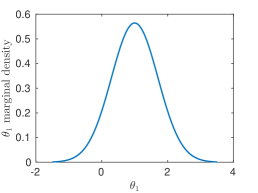
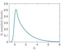
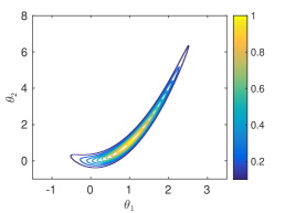
This problem is challenging to sample from since it has a highly peaked and curved ridge, and is often used as a test problem in optimisation and MCMC communities.

5.1 Implementation details

Before looking at the performance of the algorithms, we demonstrate some properties of the transport maps we will be using. We draw 1 million samples from the density (26), and use this sample in the framework of Section 3 to build a transport map. We use this map to pushforward the original sample onto the reference space, where we will be able to see how well the map has performed at converting the original sample to a standard Gaussian. We then pull the sample back on to target space using the inverse map to check that our map is invertible and well behaved.

For this example, we use an index set of total order 3 with monomial basis functions. It is important that total order is an odd number, since otherwise the map will not be surjective. This results in a map of the form

$$T(\theta_{1},\theta_{2})=\begin{bmatrix}T_{1}(\theta_{1})\\ T_{2}(\theta_{1},\theta_{2})\end{bmatrix},$$ (27)

where

$$T_{1}(\theta_{1}) =\gamma_{1,1}+\gamma_{1,2}\theta_{1}+\gamma_{1,3}\theta_{1}^{2}+\gamma_{1,4}\theta_{1}^{3},$$ (28)

$$T_{2}(\theta_{1},\theta_{2}) =\gamma_{2,1}+\gamma_{2,2}\theta_{1}+\gamma_{2,3}\theta_{1}^{2}+\gamma_{2,4}\theta_{1}^{3}+\gamma_{2,5}\theta_{2}+\gamma_{2,6}\theta_{1}\theta_{2}$$ (29)

$$\qquad\quad+\gamma_{2,7}\theta_{1}^{2}\theta_{2}+\gamma_{2,8}\theta_{2}^{2}+\gamma_{2,9}\theta_{1}\theta_{2}^{2}+\gamma_{2,10}\theta_{2}^{3}.$$ (30)

Clearly even with only basis functions of total order 3, we have a large number of unknowns in our optimisation problem, $\bar{\gamma}\in\mathbb{R}^{14}$. If we were to increase the dimension of $\theta$ further, we would need to reduce the number of terms we include in the expansion by, for example, removing all the “cross” terms. This reduces the quality of our map, but since we only require an approximate map we can afford to reduce the accuracy.

(a) Original sample $\theta$ from MH-RW algorithm.

(b) Pushforward of $\theta$ onto reference space.

(c) Pullback of reference sample onto target space.

Figure 2: The effect of the approximate transport map $\tilde{T}$ on a sample from the Rosenbrock target density as described in Equation (26).

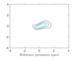
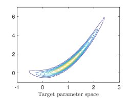
Figure 2 shows the output of the approximate transport map. Even though we have truncated the infinite expansion in the monomial basis down to 4 and 10 terms in respective dimensions, the pushforward of the sample is still a unimodal distribution centred at the origin with standard deviation 1. As one moves out into the tails of the reference density more non-Gaussian features are clearly visible. However, overall, the pushforward of the target density does not look a challenging one to sample from, with even relatively simple MCMC methods such as Metropolis-Hasting random walk (MH-RW). The pullback from reference space, in Figure 2, is an exact match of the original sample since we have not perturbed the sample in reference space. This inversion is well defined in the sampling region, although not necessarily outside it[45].

For more challenging posterior distributions, the pushforward through the numerical approximation of the optimal map often leads to a distribution on reference space which still has complex structure. It has previously been proposed that in more favourable scenarios, the optimal approach is to use independent Gaussian samples on reference space, pulled back through the inverse map. However, when the pushforward of the posterior differs greatly from this distribution, as we will see in later examples, this is not an efficient approach. Using ETAIS in conjunction with the transport map allows us to sample efficiently from the pushforward measure on reference space.

5.2 Numerical results for convergence of transport map based algorithms on the Rosenbrock density

The performance of Metropolise-Hastings methods and adaptive importance sampling methods depends on the scaling parameter $\beta^{2}$ for the proposal distributions $q(\cdot;\cdot,\beta)$. For the RW method, for example, the variance of the proposal is equal to $\beta^{2}$. We first find the optimal scaling parameters for the individual algorithms. This is done, as in [19], by optimising for the effective sample size in the ETAIS algorithm, and by tuning the relative $L^{2}$ error in the MH algorithm. The relative $L^{2}$ error of the PDF of the measure can be approximated by $E$ where

$$E^{2}=\sum\limits_{i=1}^{n_{b}}\left[\displaystyle\int_{R_{i}}\!\pi(s|D)\,\mbox{d}s-vB_{i}\right]^{2}\Big{/}\sum\limits_{i=1}^{n_{b}}\left[\displaystyle\int_{R_{i}}\!\pi(s|D)\,\mbox{d}s\right]^{2},$$ (31)

where the regions $\{R_{i}\}_{i=1}^{n_{b}}$ are the $d$-dimensional histogram bins, so that $\bigcup_{i}R_{i}\subseteq X$ and $R_{i}\cap R_{j}=\emptyset$, $n_{b}$ is the number of bins, $v$ is the volume of each bin, and $B_{i}$ is the value of the $i$th bin. This metric converges to the standard definition of the relative $L^{2}$ error as $v\rightarrow 0$.

There is currently no guidance on the best way of tuning the MH algorithm with transport map proposals, although one might expect results similar to the standard MH results, especially if adaptation of the map is stopped after a given point. As in the ETAIS algorithm, optimising for the effective sample size might be the best option.

Statistic  /  Algorithm	Transport M-H	Transport ETAIS option 1	Alg. 2
$\beta_{L^{2}}$	1.0e-0	1.1e-1	3.5e-1
$\beta_{\text{ESS}}$	-	1.0e-1	5.2e-1
Acc. rate	0.23	-	-
ESS ratio	-	0.62	0.71

Table 1: Optimal scaling parameters $\beta$ for the proposal kernels with the transport map based algorithms applied to $R_{1}$, optimising for the approximate $L^{2}$ error (31) and the effective sample size (ESS) for ETAIS algorithms, and for average acceptance rate for MH algorithms.

The optimal scaling parameters are given in Table 1. Here we see that the effective sample size is much lower than we see in the one-dimensional examples with the ETAIS algorithms. However, in the Rosenbrock density (26) we are dealing with a much more complicated curved structure, as well as a very slowly decaying tail in $\theta_{2}$. From our experiments, we have observed that the standard ETAIS-RW required an ensemble size of $M=500$ to overcome the problems in this density, however the transport map transforms the tails to be more like those of a Gaussian which can be approximated well by a smaller ensemble size of $M=150$.

(a) Comparison of the two Transport ETAIS options.

(b) Comparison of Transport ETAIS option 2 with the standard algorithms.

Figure 3: Convergence of algorithms; Transport M-H, Transport ETAIS option 1, algorithm 2 for density (26). Ensemble size $M=150$, resampling performed using the MT algorithm. Plots show average convergence over 32 repeats.

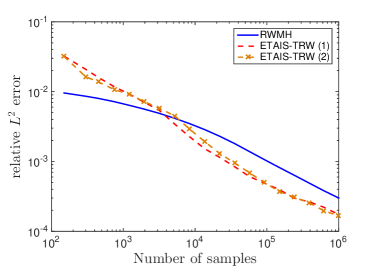
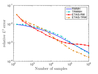
The convergence of the three algorithms is displayed in Figure 3. These convergence plots show the error as a function of the number of samples output by each algorithm. In the case of standard Metropolis-Hastings methods, this corresponds to the number of iterations. In the case of ETAIS, this corresponds to the number of iterations multiplied by the ensemble size. Figure (a) shows that the two variations of the transport based ETAIS algorithms converge with similar rates. The second version, which performs the resampling stage in reference space rather than target space, has a slightly higher ESS, and is more stable than option (1). This version also has a property that we can exploit in Section 8.1.

Figure 3 (b) compares the performance of RWMH, transport map-accelerated RWMH, ETAIS-RW and transport map-accelerated ETAIS-RW. The difference in performance between RWMH and its accelerated version is relatively negligible, in part because this version of the Rosenbrock density is not overtly tortuous. The story is different for the ETAIS algorithms. The slowly decaying tails of the Rosenbrock cause a problem for ETAIS since these are not well-represented in the proposal distributions, leading to high weight variance and poor convergence. A much larger ensemble would be required to ensure a stable ETAIS implementation for this problem, which leads to high overhead costs for the resampling step and evaluation of the importance weights. The transport map-accelerated ETAIS, on the other hand, is stabilised by the map, which transforms the proposal distributions in order to adequately approximate the slowly decaying tails of the target. This stabilisation allows us to benefit from the improved convergence of the ETAIS methodology, with a smaller ensemble size.

6 Inverse Problems for Multiscale Stochastic Chemical Reaction Networks

In this Section, we briefly introduce the idea of a continuous time Markov chain model for stochastic reaction networks. We consider the formulation of the Bayesian inference of the reaction parameters given exact data. In particular we consider the case where only slow variables in the system are observable, and hence the true likelihood function is intractable. In this case, the likelihood can be approximated using multiscale methods. The data in these scenarios is often insufficient to identify all of the parameters, and this can lead to posterior distributions which are heavily concentrated close to lower dimensional manifolds, which are challenging to sample from, and which motivated the development of the methodology outlined in this paper.

We consider chemical reaction networks of $N_{s}$ chemical species $\{S_{j}\}_{j=1}^{N_{s}}$, with population numbers given by $X(t)=[X_{1}(t),X_{2}(t),\ldots,X_{N_{s}}(t)]^{\top}\in\mathbb{N}_{0}^{N_{s}}$ reacting in a small reactor, through $N_{r}$ different reaction channels. When population numbers of one or more of the chemical species in the reactor are small, as is the case with chemical reactions occurring within living cells, the sporadic and discrete way in which reactions occur can not be well modelled by deterministic continuous models, such as ODEs. In such a situation, we may wish to model the dynamics through a discrete stochastic model, such as a continuous time Markov chain.

For each reaction $R_{j}$, for $j=1,2,\ldots N_{r}$, there is a propensity or hazard function $\alpha_{j}(X(t))$ which indicates how likely that reaction is to fire, defined by

$$\alpha_{j}(X(t))=\lim_{dt\to 0}\mathbb{P}(\text{Reaction $R_{j}$ in the time interval }\,s\in[t,t+dt]).$$ (32)

Following each reaction $R_{j}$ there is an instantaneous change in the current state, as the reactants of the reaction are consumed, and the products produced. This is modelled by a change in the state vector $X(t)=X(t)+\nu_{j}$ where $\nu_{j}$ is the stoichiometric vector for reaction $R_{j}$.

The model can be represented as the following expression involving $N_{r}$ different unit rate Poisson processes[4] $Y_{j}$, given by:

$$X(t)=X(0)+\sum_{j=1}^{N_{r}}\nu_{j}Y_{j}\left(\int_{0}^{t}\alpha_{j}(X(s))\right)ds.$$ (33)

The master equation for this model is only solvable in certain situations, for example monomolecular networks[38], or for steady-state solutions for weakly reversible deficiency zero networks[3, 2]. Trajectories for this system can be sampled exactly, for instance using the Gillespie SSA[33], or its variants[34, 12, 1].

6.1 Likelihoods arising from multiscale stochastic reaction networks

Suppose that we are able to exactly observe the number of molecules of each chemical species in a system that can be well approximated by (33). Each reaction in the system involves the firing of a Poisson process with rate which is a function of the number of reactant molecules present, and the reaction rate constants. The likelihood of each reaction is simply the product of the probability density of an exponential random variable which gives the waiting time since the last reaction, with the mass function of a multinomial distribution describing the likelihood of each type of reaction from that state. Since the reactions are assumed to be independent, the likelihood of the whole path is a product of all the individual reaction likelihoods. This can be computed in a more efficient way by considering all reactions in the data from the same point in the state space at the same time. A detailed derivation of this is given in the supplementary material.

If we are only able to observe the slow species, then we cannot write down an explicit likelihood for the path. One approach is to try to simultaneously infer the missing data of the fast variables, but this is computationally intractable in all but the simplest of cases. The other option is to invoke a multiscale approximation to the dynamics. This allows us to approximate effective propensities for the slow reactions, and hence to approximate the likelihood of paths of the slow variables. A detailed derivation of this likelihood is also given in the supplementary material.

In this work, we will consider two different multiscale approximations. The first is the quasi-equilibrium approximation which makes the assumption that fast reactions enter quasi-equilibrium on a timescale which is negligible with respect to the timescale on which the slow dynamics in the system are evolving. This approximation is the basis of several methods[28, 11]. This approach can work well when there is a large timescale gap between the fast and slow reactions in a system, but where the timescale gap is less pronounced, it can lead to significant errors[21]. Another approach is the constrained multiscale algorithm (CMA)[23, 20], based in part on the equation-free approach to multiscale computations[41, 30]. This approach also assumes quasi-equilibrium in the system, but takes into account the effect that the slow reactions can have on the invariant distribution of the fast variables in the system. For a more detailed description of this method, please refer to the literature[20].

7 Numerical Examples

In this section we consider two examples of chemical systems to demonstrate the effectiveness of transport ETAIS algorithms for sampling from the challenging posterior distribution on the reaction parameters that arise.

7.1 A Multiscale Chemical System

First we consider a simple multiscale example involving two chemical species $S_{1}$ and $S_{2}$,

$$\emptyset\xrightarrow{k_{1}}S_{1}\mathrel{\raise 1.72218pt\hbox{$\ext@arrow 3095\leftarrowfill@{\phantom{k_{3}}}{k_{2}}$}\kern-54.78061pt\lower 1.72218pt\hbox{$\ext@arrow 0359\rightarrowfill@{k_{3}}{\phantom{k_{2}}}$}}S_{2}\xrightarrow{k_{4}}\emptyset.$$ (34)

Each arrow represents a reaction from a reactant to a product, with some rate constant $k_{i}$, and where mass action kinetics is assumed. The parameters $k_{i}$ are non-negative, and $\mathbf{k}=[k_{1},\dots,k_{4}]^{\top}\in\mathbb{R}_{+}^{4}=\mathcal{X}$. We denote the population count of species $S_{i}$ by $X_{i}\in\mathbb{N}_{0}$. We consider this system with the following parameters:

$$k_{1}V=100,\qquad k_{2}=k_{3}=10,\qquad k_{4}=1,$$ (35)

where $V$ is the volume of the reactor. In this parameter regime the reactions $R_{2}\colon S_{1}\rightarrow S_{2}$ and $R_{3}\colon S_{2}\rightarrow S_{1}$ occur more frequently than the other reactions. Notice that both chemical species are involved in fast reactions. However, the quantity $S=X_{1}+X_{2}$, is conserved by both of the fast reactions, and as such, this is the slowly changing quantity in this system.

We observe this system over the time period $t\in[0,500]$ with initial condition $S_{1}(0)=S_{2}(0)=0$, but we assume that we are only able to observe the slow variable $S(t)=S_{1}(t)+S_{2}(t)$. The effective dynamics of $S$ can be approximated by a system of only two reactions:

$$\emptyset\xrightarrow{\alpha_{1}(S)}S\xrightarrow{\bar{\alpha}_{4}(S)}\emptyset,$$ (36)

where here the propensities are shown as opposed to the rates.

The effective propensity $\bar{\alpha}_{4}(S)$ can be approximated through application of a multiscale approximation, as detailed in the supplementary material, and in more detail in [20]. These effective propensities can often be computed without the need for expensive simulations, in particular when the fast subsystem is deficiency zero, which is often the case[3, 2]. For this very simple example, the dependence of these effective propensities on the original rate parameters can be explicitly understood. Under the QEA, the effective rate of degradation of the slow variable $S$ is given by

$$\bar{\alpha}_{4}^{\text{QEA}}(s)=\frac{k_{2}k_{4}s}{k_{2}+k_{3}}.$$ (37)

Similarly, the analysis of the constrained system as discussed in [20] yields the effective propensity

$$\bar{\alpha}_{4}^{\text{CMA}}(s)=\mathbb{E}_{\text{CMA}}\left[k_{4}X_{2}|S=s\right]=\frac{k_{2}k_{4}s}{k_{2}+k_{3}+k_{4}}.$$ (38)

Our observations are uninformative about the reaction rates $k_{2},k_{3}$, and $k_{4}$, as for each multiscale approximation there is a manifold $\mathcal{M}\subset\mathcal{X}$ along which the effective propensity $\hat{\alpha}_{4}$ is invariant, leading to a highly ill-posed inverse problem. This type of problem is notoriously difficult to sample from using standard MH algorithms, as the algorithms quickly gravitate towards the manifold $\mathcal{M}$ but then exploration around $\mathcal{M}$ is slow.

We aim to recover three different posterior distributions. In the first, we assume that we can fully and exactly observe the whole state vector for the whole of the observation time window $t\in[0,T]$. In the second and third, the same data are used, but projected down to one dimensional observations of the slow variable $S=X_{1}+X_{2}$. In these last two examples, we approximate the posterior using QEA and CMA approximations of the effective dynamics respectively.

In all three cases, we find the posterior distribution for $\mathbf{k}\in\mathcal{X}=\mathbb{R}_{+}^{4}$. These four parameters are assigned Gamma prior distributions,

$$k_{i}\sim\text{Gamma}(\cdot;\alpha_{i},\beta_{i}),\quad\text{for}\quad i=1,\dots,4.$$ (39)

The hyper-parameters corresponding to each of these prior distributions are given in Table 2. These priors are the same for each of the three posterior distributions.

Parameter$\backslash$Dimension $i$	1	2	3	4
$\alpha_{i}$	150	5	5	3
$\beta_{i}$	$\frac{15}{9}$	$\frac{5}{12}$	$\frac{5}{12}$	$1$

Table 2: Hyper-parameters in the prior distributions for the multiscale problem described in Section 7.1.

Figure 4: CMA approximation of the posterior arising from observations of the slow variable $S=X_{1}+X_{2}$ for system (34) with true rates given by (35).

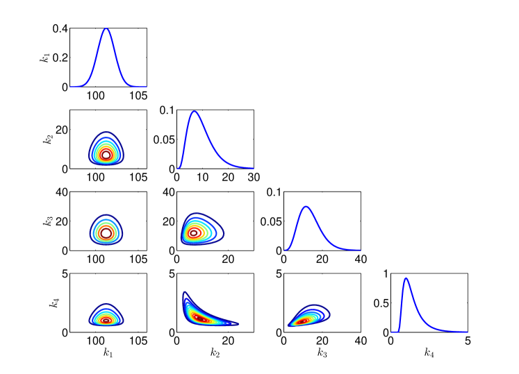
Figure 4 shows how this posterior looks when we use the CMA to model the effective degradation propensity $\bar{\alpha}_{4}$. Although this posterior does not appear to be impenetrably difficult to sample using MCMC from these plots, it most certainly is. The posterior density is concentrated close to a curved manifold. Since the manifold is curved, the joint marginals do not look unreasonable. However, the distribution is highly peaked around this curved manifold, making it very difficult to sample from efficiently.

We consider several different algorithms for sampling from these distributions. First we implement both the ETAIS and MH algorithms with a Gaussian proposal distribution. In the case of the ETAIS algorithm, this is a Gaussian mixture proposal distribution, and in the MH algorithm this is equivalent to a “vanilla” random walk. The proposal distribution uses a covariance matrix which has been constructed using the sample covariance of a sample produced using a standard MH-RW algorithm. This is necessary since these algorithms otherwise fail to converge in a reasonable time for this problem. We also compare the ETAIS and MH algorithms when using a transport map proposal distribution, as was discussed in detail in Chapter 4.

In practice we cannot ensure that the approximate map $\tilde{T}$ is uniquely invertible over the whole of $R$ and so $\tilde{T}$ is not truly bijective. This leads to problems for our strictly positive state space, $\mathcal{X}\subset\mathbb{R}_{+}^{d}$, and so proposals in $R$ do not necessarily map back onto $\mathcal{X}$. This can be avoided, however, by employing a logarithmic preconditioner for the transport map. The proposal distributions are labelled with a T for transport map and when using the intermediate space we prepend ‘log’ to the proposal method, e.g. MH-logRW and MH-logTRW, with, ETAIS-logRW and ETAIS-logTRW.

The inclusion of the composition with the logarithmic map means that we must alter our importance weight definition to reflect the pullback from $R$ through $\mathcal{Y}$. The weight is now

$$w_{i}(\theta)=\frac{\pi(\theta|\mathbf{R},\mathbf{T})}{\chi(\tilde{T}\circ\log(\theta)|\tilde{T}\circ\log(\theta^{(i-1)}))|J_{\tilde{T}\circ\log}(\theta)|},$$ (40)

where $\theta$ is a proposed new state, $\theta^{(i-1)}$ is the ensemble of states from the previous iteration, and $J_{\tilde{T}\circ\log}(\theta)$ is the Jacobian of the composition of the two maps. This Jacobian is straightforward to calculate,

$$|J_{\tilde{T}\circ\log}(\theta^{\prime})|=|J_{\tilde{T}}(\log(\theta^{\prime}))||J_{\log}(\theta^{\prime})|,$$ (41)

where the first determinant is computed as in (13), and the second is given by

$$|J_{\log}(\theta^{\prime})|=\prod\limits_{i=1}^{d}\frac{1}{\theta^{\prime}_{i}}.$$ (42)

For this problem, we continue to use monomials in each dimension in our transport map construction. We use polynomials of total order $p=3$ as the basis functions, i.e.

$$T_{i}(\theta)=\sum_{\mathbf{j}\in\mathcal{J}^{\text{TO}}_{i}(p)}\gamma_{i,\mathbf{j}}\psi_{\mathbf{j}}(\theta)\quad\text{where}\quad\psi_{\mathbf{j}}(\theta)=\prod\limits_{k=1}^{i}\theta_{k}^{j_{k}},$$ (43)

and

$$\mathcal{J}^{\text{TO}}_{i}(p)=\{\mathbf{j}\in\mathbb{N}^{d}_{0}\ |\ \|\mathbf{j}\|_{1}\leq p,\ \text{and}\ j_{k}=0\ \forall k>i\}.$$ (44)

We will use the MT[48] resampler with an ensemble size of $M=500$. This increase in ensemble size in comparison with the previous example in Section 5 is to allow for the increase in parameter dimension.

To measure the convergence of the sampling methods in this section, we will compare the convergence of the mean of each parameter. We approximate $\mathbb{E}(\mathbf{k})$ using 2.4 billion samples from the MH-RW algorithm. We do this for each of the eight algorithms we have so far discussed. Convergence is shown only for the CMA approximation of the posterior with effective rate for the degradation of $S$ given by (38), but we expect very similar results for the other multiscale approximation of posterior distributions discussed.

	MH		ETAIS
	logRW	log-TRW	logRW	log-TRW
$\beta_{\%}^{*}$	1.7e-1	2.7e-2	-	-
$\beta_{\text{ESS}}^{*}$	-	-	1.2e-0	1.5e-1
ESS/$M$	-	-	6.0e-2	3.5e-1

Table 3: Optimal scaling parameters for the MH and ETAIS algorithms applied to the constrained multiscale problem in Section 7.1. MH parameters optimised by acceptance rate, and ETAIS parameters optimised using effective sample size. ESS per sample also shown for the ETAIS algorithms.

The optimal scaling parameters for the proposal distributions are given in Table 3. These are precomputed by running the algorithms for different parameter values. MH-RW based algorithms are tuned to an acceptance rate close to the optimal $23.4\%$, and ETAIS algorithms are tuned to maximise the effective sample size (ESS). The optimal parameter values for the MH algorithms are not particularly informative about their performance, since they relate to algorithms operating on different transformations. The ESS per sample is also displayed in Table 3 for the ETAIS implementations, and is highest for the logTRW variant of the ETAIS algorithm, as we would hope. We note here that, as outlined in [19], it is possible to construct adaptive versions of ETAIS which automatically tune these algorithmic parameters, but we compare against the static optimal parameter values for all algorithms to ensure fairness.

Figure 5: Convergence of four different MCMC algorithms for the CMA approximation of the posterior arising from the example in Section 7.1. Plots show average convergence over 32 repeats.

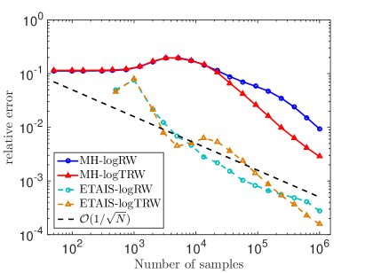
Convergence of the four algorithms for this example are shown in Figure 5. We first note the poor performance of the MH based algorithms, despite being preconditioned with a pre-computed sample covariance. Only the MH-TRW is at all competitive with the ETAIS algorithms. During the simulation interval, the MH-TRW algorithm has not settled down to the expected $\mathcal{O}(1/\sqrt{N})$ rate which means that the estimate is still biased by the long burn-in time. As we have seen in previous examples, the burn-in time for the ETAIS algorithm is negligible.

This proposal method becomes more stable as we increase either the ensemble size, or the number of iterations between updates of the transport map, $T$. Overall we see the smallest Monte Carlo errors for a given number of likelihood evaluations coming from the ETAIS-logTRW algorithm. This is due to weight collapse in some of the 32 repeats of the ETAIS-logRW algorithm, demonstrating that the transport map stabilises the ETAIS methodology.

(a) Pushforward of the posterior sample through $\hat{T}$ with log preconditioner.

Figure 6: Pushforward of the target measure on reference space for the CMA approximation of the posterior arising from the example in Section 7.1, found using the logTRW proposal distributions. Components are linked by the relation $r_{i}=T_{i}\circ\log(k_{i})$.

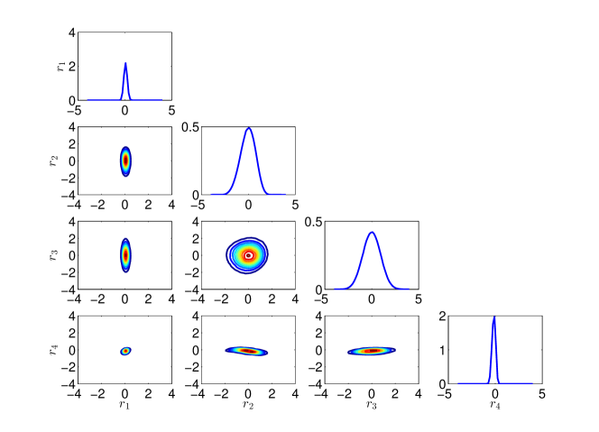
We now look at the proposal distributions of the transport map accelerated algorithm. In Figure 6, we see the reference space found by mapping the posterior through $T\circ\log$. For the most part, each of these marginal distributions can be recognised as a Gaussian. However, with the exception of $\mathbb{P}(r_{2},r_{3})$, we would not consider them to be close to a standardised $\mathcal{N}(0,\text{I})$ distribution. Before thinking that the transport map has not helped us to find a ‘nicer’ space on which to propose new values we should consider that the dimensions are now (1) largely uncorrelated, and (2) the variances in each dimension are much more similar than they are in Figure 4.

We see that $\text{var}(r_{1})$ and $\text{var}(r_{4})$ are much smaller than $\text{var}(r_{2})$ and $\text{var}(r_{3})$. To combat this we have a number of choices. We might wish to learn the covariance structure of the pushforward of the target onto the reference space, and incorporate this information into the covariances of the mixture components in an adaptive scheme. Another option is to increase the total order of our index set. For these numerics we have chosen $p=3$, but we can obtain reference spaces which are closer to $\mathcal{N}_{d}(0,\text{I})$ by choosing a larger $p$.

At this point, we note that if the transport map found is equal or close to the Knothe-Rosenblatt rearrangement, then the most efficient sampling strategy is clearly to independently sample from the reference measure and pull these samples back through the map onto (or close to) the target. However we see from Figure 6 that in practice for very complex targets, the approximation of the transport map is not as good, and as such the pushforward of the target onto the reference space differs greatly from the intended reference measure. In this case, the pullback of the reference measure will be far from the target distribution, and this independent sampling strategy will be inefficient. This motivates the use of the ETAIS algorithm to efficiently sample from the more complex distributions arising from the pushforward of the target distribution.

7.1.1 Comparison of the Constrained and QEA approaches

The convergence analysis in the previous section was performed for the constrained approximation of the posterior distribution. We now look at the differences in the CMA and QEA approximations of the posterior distribution arising in this problem. Recall that the approaches differed only in the form of the effective degradation propensity $\hat{\alpha}_{4}$,

$$\hat{\alpha}_{4}^{\text{QEA}}(s)=\frac{k_{2}k_{4}s}{k_{2}+k_{3}}\quad\text{and}\quad\hat{\alpha}_{4}^{\text{CMA}}(s)=\frac{k_{2}k_{4}s}{k_{2}+k_{3}+k_{4}}.$$ (45)

This difference in the denominator causes a shift in the manifold on which the posterior is concentrated.

In the QEA approximation, the effective rate of degradation of $S$ is given by $\hat{k}_{4}^{\text{QEA}}=k_{2}k_{4}/(k_{2}+k_{3})$, and as such, our observations should be informative about this quantity. Using the CMA, this effective rate is approximated by $\hat{k}_{4}^{\text{CMA}}=k_{2}k_{4}/(k_{2}+k_{3}+k_{4})$. To validate our inferences on $k_{2}$, $k_{3}$ and $k_{4}$ we would like to discover which model is most accurate and informative about these quantities, and which model gives us results which are most similar to that which can be obtained from the full model, with all reactions (including fast reactions) observed.

A conventional way to compare two models under a Bayesian framework is to calculate the Bayes factors [15]. The marginal densities for the data, evaluated at the observed data, given the models are displayed in Table 4.

Model description	$k$	$\mathbb{P}(D=(\mathbf{R},\mathbf{T})^{\top}|\mathcal{M}_{k})$	Bayes’ factor
Full	0	6.8e-3	1
CMA	1	3.2e-3	2.09
QEA	2	1.7e-3	4.10

Table 4: Marginal distributions and Bayes factors for the data $(\mathbf{R},\mathbf{T})^{\top}$ for each model considered in Section 7.1. The Bayes’ factors are computed with respect to the “full” model.

Computing the Bayes factors from Table 4 we see that we should of course prefer the model in which we observe all reactions perfectly and are able to explicitly compute the likelihood. However this model is not significantly better than the CMA model ($B_{0,1}=2.09<3.2$,  [40]). The Bayes factor $B_{0,2}=4.1>3.2$ tells us that we should significantly prefer the full model to the QEA approximation of the posterior. These Bayes factors provide evidence for our argument that the constrained approximation of the posterior is superior to the QEA approximation.

(a) Marginal for $\hat{k}_{4}^{\text{QEA}}$.

(b) Marginal for $\hat{k}_{4}^{\text{CMA}}$.

Figure 7: Comparison of the approximate marginal densities for the quantities $\hat{k}_{4}^{\text{QEA}}$ and $\hat{k}_{4}^{\text{CMA}}$ across the three posterior densities $\pi_{i}=\mathbb{P}(\theta_{i}|D,\mathcal{M}_{i})$ for $i=0,1,2$.

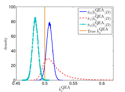
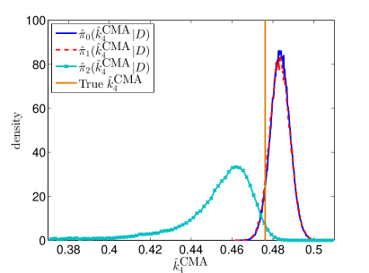
Figure 7 displays more compelling evidence in this direction. Here we show the marginal distributions for the quantities $\hat{k}_{4}^{\text{QEA}}$ and $\hat{k}_{4}^{\text{CMA}}$ with respect to each of the three posterior distributions, $\pi_{i}(\cdot|D,\mathcal{M}_{i})$, $i=0,1,2$. Firstly, in Figure 7 (a), displaying the marginals for $\hat{k}_{4}^{\text{QEA}}$ we see that $\pi_{0}$, the density arising from the full model with all reactions observed, is peaked a distance away from $\pi_{2}$, QEA approximation. The CMA approximation $\pi_{1}$, in contrast, is peaked close to peak of $\pi_{0}$, but there is more uncertainty here since we do not observe the fast reactions.

In contrast, in Figure 7 (b), the marginal densities for $\hat{k}_{4}^{\text{CMA}}$ for $\pi_{0}$ and $\pi_{1}$ are barely distinguishable, even with the vastly reduced data available in the posterior $\pi_{1}$ with CMA approximation. The QEA approximation $\pi_{2}$ is again peaked far away from both of the other distributions. This demonstrates that the data regarding the slow variable $S$ is only informative about $k_{1}$ and $\hat{k}_{4}^{\text{CMA}}$, as predicted by the constrained multiscale approximation.

7.2 Gene Regulatory Network

In this example, we look at a model of a gene regulatory network (GRN) mechanism [39, 36, 6] used by a cell to regulate the amount of a protein, $P$, present. Proteins can bind in pairs to form a dimer $D$. The dimer can bind to the gene $G$ and convert it into a “switched off” state $G^{\prime}$, in which the production of mRNA molecules $M$ is inhibited. The mRNA encodes for production of the protein $P$, and both $P$ and $M$ can degrade. The eight reactions are given in Equation (46).

$$P+P\mathrel{\raise 1.72218pt\hbox{$\ext@arrow 3095\leftarrowfill@{\phantom{k_{2}}}{k_{1}}$}\kern-54.78061pt\lower 1.72218pt\hbox{$\ext@arrow 0359\rightarrowfill@{k_{2}}{\phantom{k_{1}}}$}}D\quad \quad G+D\mathrel{\raise 1.72218pt\hbox{$\ext@arrow 3095\leftarrowfill@{\phantom{k_{4}}}{k_{3}}$}\kern-54.78061pt\lower 1.72218pt\hbox{$\ext@arrow 0359\rightarrowfill@{k_{4}}{\phantom{k_{3}}}$}}G^{\prime}$$

$$G\xrightarrow{k_{5}}G+M\quad \quad M\xrightarrow{k_{6}}M+P$$ (46)

$$P\xrightarrow{k_{7}}\emptyset\quad \quad M\xrightarrow{k_{8}}\emptyset$$

We create trajectories of this system, using the Gillespie SSA, with the following parameters:

$$k_{1}=0.04,\qquad k_{2}=5000,\qquad k_{3}=100,\qquad k_{4}=1,$$ (47)

$$k_{5}=0.5,\qquad k_{6}=2,\qquad k_{7}=0.2,\qquad k_{8}=0.05,$$ (48)

over the time period $t\in[0,500]$.

T-cells can be manufactured which bind to proteins of a certain type, and cause them to phosphoresce, allowing for approximate observations of the concentration levels of that protein. However, the T-cells will not necessarily differentiate between monomers and dimers of the protein. We approximately replicate such a scenario, in a zero-observational noise setting, by assuming that we can only observe $T=P+2D+2G^{\prime}$, the total number of protein molecules in the system, alongside $M$, the concentration of mRNA. The number of dimers, and the status of the genetic switch, are assumed unobservable. In order to sample from the posterior distribution on the reaction parameters in the system given these observations, we can either integrate over all possible trajectories of the fast variables (which is computationally intractable), or as in Section 7.1 we can use a multiscale method to approximate the posterior.

The effective dynamics of $T$ and $M$ are then given by:

$$\emptyset\xrightarrow{\hat{\alpha}_{5}}M\quad \quad M\xrightarrow{\alpha_{6}}M+T$$ (49)

$$T\xrightarrow{\hat{\alpha}_{7}}\emptyset\quad \quad M\xrightarrow{\alpha_{8}}\emptyset$$

Here, the propensities are displayed, as opposed to the rates, with approximations of the propensities $\hat{\alpha}_{5}$ and $\hat{\alpha}_{7}$ to be computed. We omit the derivation of these effective propensities, using the CMA methodology, for brevity, but interested readers can see more details in [48].

7.2.1 Target Distribution

As alluded to in the previous section, we aim to sample from the CMA approximation of the posterior distribution. This example is more involved than the previous one, since we have an eight dimensional parameter space corresponding to the eight reaction rates in the system (46). Half of those reactions are unobservable, and their effect on the posterior is only felt through their effect on the effective propensities $\hat{\alpha}_{5}$ and $\hat{\alpha}_{7}$, and observations of the frequencies of these reactions.

The priors for this problem were chosen to be fairly uninformative, and a list of the hyper-parameters corresponding to each Gamma prior can be found in Table 5.

Dimension $i$	1	2	3	4	5	6	7	8
$\alpha_{i}$	2	100	100	3	3	3	2	2
$\beta_{i}$	50	0.02	1	1	0.6	1	50	50

Table 5: Hyper parameters for the Gamma priors on each of the reaction rates in the GRN example in Section 7.2.

Figure 8: Marginal densities of the CMA approximation of the posterior distribution for the GRN example in Section 7.2.

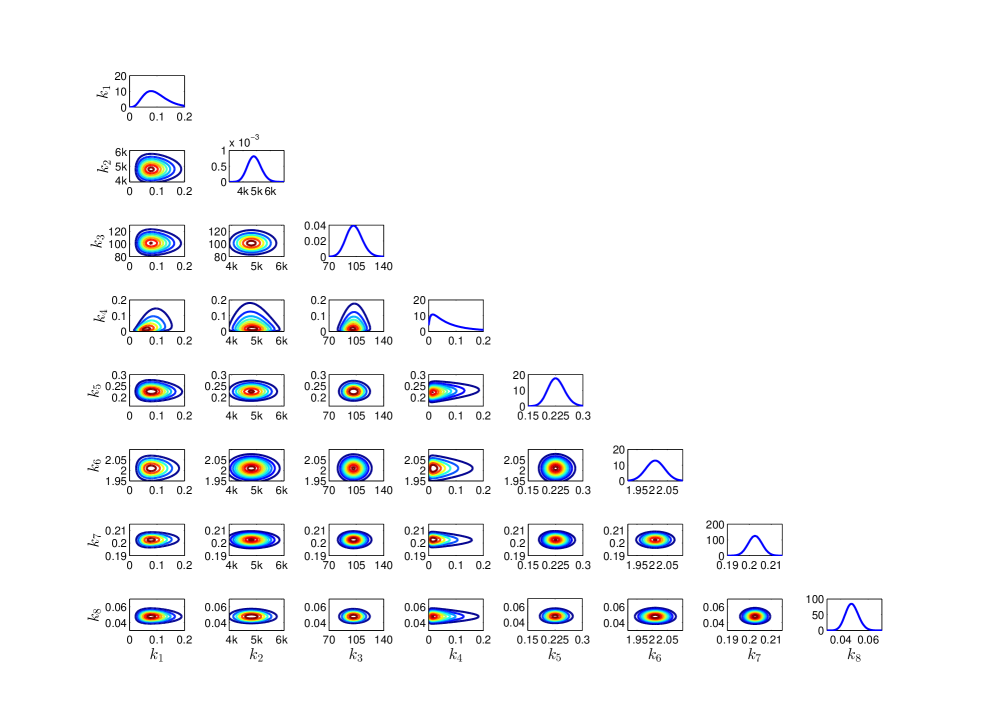
The one- and two-dimensional marginal distributions for the full posterior distribution are displayed in Figure 8. The posterior does not appear from these joint marginals to contain many interesting correlation structures, although several dimensions have leptokurtic tails, which are difficult for the standard ETAIS algorithm to sample from. However as with the previous example, the density is concentrated close to a lower-dimensional curved manifold. The marginal densities also vary over very different scales, which could lead to problems with the algorithms which do not benefit from the transport map.

7.2.2 Implementation

We apply the four logRW proposal distributions, with and without transport map acceleration, which were discussed in Section 7.1 to this posterior. As with this example, the log conditioner is required so that our transport map is a function $T\colon\mathbb{R}^{d}\rightarrow\mathbb{R}^{d}$, rather than a map from $\mathbb{R}_{+}^{d}$ to $\mathbb{R}^{d}$.

The transport map setup has not changed from the previous example. However, due to the scaling of the weights we have had to be more careful about which samples we use to build our map. We require that the objective function $C(T)$, from Equation (16) is convex, which requires that the second derivative, given in Equation (23), is positive definite. This positive definite property depends on all weights in our sample being strictly positive, which is not always possible on a computer, where very small positive numbers can be rounded down to absolute zero. For this reason we filter out any samples from the optimisation problem where the weight is a numeric zero. This does not affect the validity of the map since a weight zero would not contribute to the expectation.

In all four algorithms we adapt the proposal variances during the burn-in phase of the algorithms to avoid the need for a huge ensemble size to approximate the posterior with a mixture of isotropic Gaussian kernels. We use the MT resampler, this time with an ensemble size of $M=2500$. The increase in ensemble size compensates for the increase in dimension from four to eight.

As in the previous chemical reaction example, we measure convergence of the algorithms only through the convergence of the mean. We use the sample Mahalanobis distance, with ‘true’ covariance and ‘true’ mean built from a sample of size 2.4 billion using the MH-RW algorithm.

7.2.3 Convergence results

The scaling parameters used are selected by optimising the acceptance rate for the MH algorithms, and optimising the effective sample size for the ETAIS algorithms. The optimal parameters are given in Table 6. Here, for Metropolis-Hastings variants, $\beta_{\%}^{*}$ is the variance of the proposal, optimised for an acceptance rate of $50\%$. For the ETAIS variants, $\beta_{\text{ESS}}^{*}$ is the variance of each of the proposal kernels around each particle, optimised numerically for the maximal effective sample size (ESS). ESS/$M$ denotes the ratio of ESS to the number of particles, with values closer to one denoting a more efficient algorithm.

	MH		ETAIS
	logRW	log-TRW	logRW	log-TRW
$\beta_{\%}^{*}$	3.9e-1	6.0e-1	-	-
$\beta_{\text{ESS}}^{*}$	-	-	1.3e-0	5.0e-1
ESS/$M$	-	-	4.7e-2	1.6e-1

Table 6: Scaling parameters for the sampling algorithms applied to the GRN example in Section 7.2.

From the effective sample sizes shown in Table 6 we can see the improvement to the efficiency of the algorithm both by transforming the parameter space into something closer to Gaussian.

Due to the numerical cost of calculating the full relative $L^{2}$ errors for this posterior, we quantify the convergence speeds of these algorithms using the sample Mahalanobis distance between the sample mean and the ‘true’ mean. This convergence analysis is shown in Figure 9.

Figure 9: Convergence of four different MCMC algorithms for the CMA approximation of the posterior arising from the example in Section 7.2. Plots show average convergence over 32 repeats.

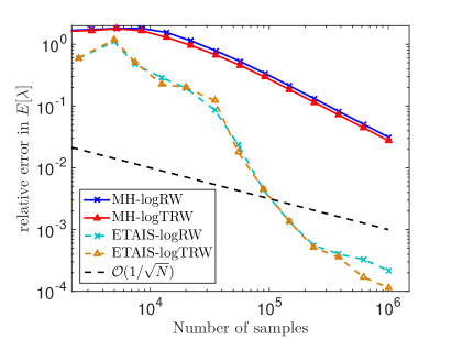
We believe that an ensemble size of 2500 is over-cautious, despite the larger number of dimensions in this example, and that the required ensemble size to sample from these posteriors is reduced by the use of the transport map.

The second obvious feature of these convergence plots is that the ETAIS algorithms outperform the MH algorithms by a large margin - roughly a reduction of two orders of magnitude in the relative error over the same number of samples.

The transport map version exhibits more consistent and stable convergence, with some of the 32 repeats for the ETAIS-logRW algorithm producing rare large weights which hinder convergence. The large increase in the effective sample size observed between the ETAIS-logRW and ETAIS-logTRW algorithms is converted into an estimate which is twice as accurate after 1 million samples. This corroborates with our claim that the transport map can produce stable ETAIS implementations with smaller ensemble sizes than without.

A similar pattern is seen in the MH algorithms, where the MH-logTRW algorithm performs the best, although only marginally.

8 Discussion

In this paper, we have investigated the use of transport maps to accelerate and stabilise ensemble importance sampling schemes. We considered the ETAIS methodology here, but the approach used is applicable to all such methods. The idea is powerful since it allows adaptive importance sampling schemes to be efficient and stable for smaller ensemble sizes. This in turn suggests that the improvements in performance that adaptive importance sampling schemes can deliver could be made applicable to a bigger class of problems.

If good transport maps can be found, such that the pushforward of the posterior is close to a reference Gaussian, then the most efficient approach is to draw independent samples pulled back through the map onto the target space. However, for complex posteriors, in particular the type that we have observed here where due to sloppiness in the model, the posterior is concentrated on a low-dimensional manifold, a good map is hard to find. The numerical approximation of the optimal map leads to a measure on the reference space which is far removed from the reference Gaussian, and requires more considered exploration. Adaptive importance sampling schemes such as ETAIS are able to sample from such a measure more efficiently than Metropolis-Hastings equivalents.

One issue that we have not looked at in depth, is that of the choice of basis functions for the transport map, which is discussed in more depth in [45]. It seems reasonable to expect that this choice could have an impact on the quality of the transport map, which in turn has an impact on the number of ensemble members which are required to stably sample from the target distribution. We explored some different combinations, including higher order but sparse bases, but we did not observe a big difference in performance. It would be an interesting avenue to explore how other approaches, for example tailored, anisotropic, or even adaptively chosen parameterisations, could enable the map to more accurately capture the structure of the target density, reducing the required ensemble size.

In particular we looked at the application of these methods to problems arising in inverse problems for multiscale stochastic chemical networks, where the posterior distributions which arise can be highly concentrated along curved manifolds in parameter space. Through these results we also demonstrated the improvement in accuracy of inference for multiscale problems when more sophisticated multiscale approximations are employed. Below we highlight two areas for future work.

8.1 Sampling in higher dimensions

One major issue with importance sampling-based algorithms is the curse of dimensionality. This curse is two-fold, since as the target distribution’s dimension is increased, a larger ensemble size is often required in order to capture the addition complexity of the density that the higher dimension enables. Furthermore, the cost of the resampling step within the algorithm grows with the ensemble size. For example, the ETPF algorithm is $\mathcal{O}(n^{2})$. However, the simplification that the transport map makes has some potential to go some way to tackling this problem.

Here, we will briefly discuss how transport maps could aid with making moderately higher dimensional problems accessible to this family of methods. It is important to emphasise here that these methods are unlikely to be suitable in anything other than low dimensional problems, but the idea that we present here, which is the subject of future investigation, could make them applicable to more problems which have more than a handful of parameters.

Armed with a high quality transport map, we can transform the target distribution close to a Gaussian reference measure, which is approximately uncorrelated in all dimensions. This lack of correlations allows us to resample in each dimension separately. Resampling in a single dimension allows for optimisations in resampling code, and also means that the resampler is not affected by the curse of dimensionality.

In one dimension, the ETPF algorithm can be implemented very efficiently. As described in [47], the coupling matrix has all non-zero entries in a staircase pattern when the state space is ordered. We can exploit this knowledge to produce Algorithm 3, which is much faster than using the simplex algorithm to minimise the associated cost function, and faster than the MT algorithm[19], which is itself a greedy approximation to the output of the ETPF resampler. Moreover, the task of running this resampler can then be parallelised over $d$ processors. This could be an area for further study.

1 Sort the states, $\{(w_{i},x_{i})\}_{i=1}^{M}$, into ascending order.

2 Normalise the weights $p_{i}=w_{i}/\|w\|_{1}$.

3 Set $y_{i}\leftarrow 0$ for all $i=1,\dots,M$.

4 Set $c\leftarrow 0$

5 for $i\leftarrow 1,\dots,M$ do

6       Set $t\leftarrow p_{i}$

7       while $j\leq M$ and $t>0$ do

8             Set $s\leftarrow\left(M^{-1}-c\right)\wedge t$

9             Increase $y_{j}$ by $M\times s\times x_{i}$.

10             Decrease $t$ by $s$.

11             Increase $c$ by $s$.

12             if $t>0$ then

13                   Increase $j$ by 1.

14                   Set $c\leftarrow 0$.

15            

16      

17Return $y$.

Algorithm 3 ETPF algorithm in one dimension.

8.2 Adaptivity of ensemble sizes

At initialisation, our transport map approximation is equal to the identity, and the algorithm is essentially the standard ETAIS algorithm. In order to build a good transport map approximation, we require a good sample from the posterior distribution. Since our aim is to apply this methodology to challenging problems, this is itself a challenge. However, in the limit of the number of ensemble members going to infinity, this approach is consistent and stable. However, large ensemble sizes come with large computational costs.

We propose that the transport map acceleration could be used in conjunction with an adaptive ensemble size mechanism. First we can initialise the algorithm with a large ensemble size, and the identity transport map. As we explore the density, the transport map quickly improves, making it possible to sample efficiently and stably with a smaller ensemble size. The problem then amounts to finding a reliable method to approximate the lowest stable ensemble size.

References

- [1] D. Anderson, A modified next reaction method for simulating chemical systems with time dependent propensities and delays, The Journal of chemical physics, 127 (2007), p. 214107.
- [2] D. Anderson and S. Cotter, Product-form stationary distributions for deficiency zero networks with non-mass action kinetics, Bulletin of mathematical biology, 78 (2016), pp. 2390–2407.
- [3] D. Anderson, G. Craciun, and T. Kurtz, Product-form stationary distributions for deficiency zero chemical reaction networks, Bulletin of mathematical biology, 72 (2010), pp. 1947–1970.
- [4] D. Anderson and T. Kurtz, Continuous time markov chain models for chemical reaction networks, in Design and analysis of biomolecular circuits, Springer, 2011, pp. 3–42.
- [5] J. Apgar, D. Witmer, F. White, and B. Tidor, Sloppy models, parameter uncertainty, and the role of experimental design, Molecular BioSystems, 6 (2010), pp. 1890–1900.
- [6] A. Becskei and L. Serrano, Engineering stability in gene networks by autoregulation, Nature, 405 (2000), p. 590.
- [7] J. Bierkens, P. Fearnhead, and G. Roberts, The zig-zag process and super-efficient sampling for bayesian analysis of big data, arXiv preprint arXiv:1607.03188, (2016).
- [8] V. Bogachev, A. Kolesnikov, and K. Medvedev, Triangular transformations of measures, Sbornik: Mathematics, 196 (2005), p. 309.
- [9] A. Bouchard-Côté, S. Vollmer, and A. Doucet, The bouncy particle sampler: A nonreversible rejection-free markov chain monte carlo method, Journal of the American Statistical Association, (2018), pp. 1–13.
- [10] M. Bugallo, V. Elvira, L. Martino, D. Luengo, J. Miguez, and P. Djuric, Adaptive importance sampling: the past, the present, and the future, IEEE Signal Processing Magazine, 34 (2017), pp. 60–79.
- [11] Y. Cao, D. Gillespie, and L. Petzold, The slow-scale stochastic simulation algorithm, The Journal of chemical physics, 122 (2005), p. 014116.
- [12] Y. Cao, H. Li, and L. Petzold, Efficient formulation of the stochastic simulation algorithm for chemically reacting systems, The journal of chemical physics, 121 (2004), pp. 4059–4067.
- [13] O. Cappé, R. Douc, A. Guillin, J. Marin, and C. Robert, Adaptive importance sampling in general mixture classes, Statistics and Computing, 18 (2008), pp. 447–459.
- [14] O. Cappé, A. Guillin, J. Marin, and C. Robert, Population Monte Carlo, Journal of Computational and Graphical Statistics, (2012).
- [15] M. Chen, Q. Shao, and J. Ibrahim, Monte Carlo methods in Bayesian computation, Springer Science & Business Media, 2012.
- [16] E. Chiavazzo, R. Covino, R. Coifman, C.W. Gear, A. Georgiou, G. Hummer, and I. Kevrekidis, Intrinsic map dynamics exploration for uncharted effective free-energy landscapes, Proceedings of the National Academy of Sciences, 114 (2017), pp. E5494–E5503.
- [17] P. Constantine, E. Dow, and Q. Wang, Active subspace methods in theory and practice: applications to kriging surfaces, SIAM Journal on Scientific Computing, 36 (2014), pp. A1500–A1524.
- [18] J. Cornuet, J. Marin, A. Mira, and C. Robert, Adaptive multiple importance sampling, Scandinavian Journal of Statistics, 39 (2012), pp. 798–812.
- [19] C. Cotter, S. Cotter, and P. Russell, Ensemble Transport Adaptive Importance Sampling, Submitted to SIAM Journal on Uncertainty Quantification, (2019).
- [20] S. Cotter, Constrained approximation of effective generators for multiscale stochastic reaction networks and application to conditioned path sampling, Journal of Computational Physics, 323 (2016), pp. 265–282.
- [21] S. Cotter and R. Erban, Error analysis of diffusion approximation methods for multiscale systems in reaction kinetics, SIAM Journal on Scientific Computing, 38 (2016), pp. B144–B163.
- [22] S. Cotter, G. Roberts, A. Stuart, and D. White, MCMC methods for functions: modifying old algorithms to make them faster, Statistical Science, 28 (2013), pp. 424–446.
- [23] S. Cotter, K. Zygalakis, I. Kevrekidis, and R. Erban, A constrained approach to multiscale stochastic simulation of chemically reacting systems, The Journal of Chemical Physics, 135 (2011), p. 094102.
- [24] R. Douc, A. Guillin, J. Marin, and C. Robert, Convergence of adaptive mixtures of importance sampling schemes, The Annals of Statistics, 35 (2007), pp. 420–448.
- [25] R. Douc, A. Guillin, J-M Marin, and C. Robert, Minimum variance importance sampling via population monte carlo, ESAIM: Probability and Statistics, 11 (2007), pp. 427–447.
- [26] C. Dsilva, R. Talmon, C.W. Gear, R. Coifman, and I. Kevrekidis, Data-driven reduction for a class of multiscale fast-slow stochastic dynamical systems, SIAM Journal on Applied Dynamical Systems, 15 (2016), pp. 1327–1351.
- [27] S. Duane, A. Kennedy, B. Pendleton, and D. Roweth, Hybrid Monte Carlo, Physics letters B, 195 (1987), pp. 216–222.
- [28] W. E, D. Liu, and E. Vanden-Eijnden, Nested stochastic simulation algorithms for chemical kinetic systems with multiple time scales, Journal of computational physics, 221 (2007), pp. 158–180.
- [29] T. El Moselhy and Y. Marzouk, Bayesian inference with optimal maps, Journal of Computational Physics, 231 (2012), pp. 7815–7850.
- [30] R. Erban, I. Kevrekidis, D. Adalsteinsson, and T. Elston, Gene regulatory networks: A coarse-grained, equation-free approach to multiscale computation, The Journal of chemical physics, 124 (2006), p. 084106.
- [31] P. Flandrin, P. Borgnat, and P-O Amblard, From stationarity to self-similarity, and back: Variations on the lamperti transformation, in Processes with Long-Range Correlations, Springer, 2003, pp. 88–117.
- [32] C. Gardiner, Stochastic methods, vol. 4, springer Berlin, 2009.
- [33] D. Gillespie, Exact stochastic simulation of coupled chemical reactions, The Journal of Physical Chemistry, 81 (1977), pp. 2340–2361.
- [34] , Stochastic simulation of chemical kinetics, Annu. Rev. Phys. Chem., 58 (2007), pp. 35–55.
- [35] M. Girolami and B. Calderhead, Riemann manifold langevin and hamiltonian monte carlo methods, Journal of the Royal Statistical Society: Series B (Statistical Methodology), 73 (2011), pp. 123–214.
- [36] N. Guido, X. Wang, D. Adalsteinsson, D. McMillen, J. Hasty, C. Cantor, T. Elston, and J. Collins, A bottom-up approach to gene regulation, Nature, 439 (2006), p. 856.
- [37] R. Gutenkunst, J. Waterfall, F. Casey, K. Brown, C. Myers, and J. Sethna, Universally sloppy parameter sensitivities in systems biology models, PLoS computational biology, 3 (2007), p. e189.
- [38] T. Jahnke and W. Huisinga, Solving the chemical master equation for monomolecular reaction systems analytically, Journal of Mathematical Biology, 54 (2007), pp. 1–26.
- [39] M. Kaern, T. Elston, W. Blake, and J. Collins, Stochasticity in gene expression: from theories to phenotypes, Nature reviews. Genetics, 6 (2005), p. 451.
- [40] R. Kass and A. Raftery, Bayes factors, Journal of the American Statistical Association, 90 (1995), pp. 773–795.
- [41] I. Kevrekidis, C.W. Gear, J. Hyman, P. Kevrekidis, O. Runborg, C. Theodoropoulos, et al., Equation-free, coarse-grained multiscale computation: Enabling mocroscopic simulators to perform system-level analysis, Communications in Mathematical Sciences, 1 (2003), pp. 715–762.
- [42] L. Martino, V. Elvira, D. Luengo, and J. Corander, An adaptive population importance sampler: Learning from uncertainty, IEEE Transactions on Signal Processing, 63 (2015), pp. 4422–4437.
- [43] , Layered adaptive importance sampling, Statistics and Computing, 27 (2017), pp. 599–623.
- [44] Y. Marzouk, T. Moselhy, M. Parno, and A. Spantini, Handbook of Uncertainty Quantification, Springer, 2017, ch. An introduction to sampling via measure transport.
- [45] M. Parno and Y. Marzouk, Transport map accelerated markov chain monte carlo, SIAM/ASA Journal on Uncertainty Quantification, 6 (2018), pp. 645–682.
- [46] M. Pinsker, Information and information stability of random variables and processes, (1960).
- [47] S. Reich, A nonparametric ensemble transform method for Bayesian inference, SIAM Journal on Scientific Computing, 35 (2013), pp. A2013–A2024.
- [48] P. Russell, Parallel MCMC methods and their application in inverse problems, PhD thesis, School of Mathematics, University of Manchester, 2017.
- [49] A. Singer and R. Coifman, Non-linear independent component analysis with diffusion maps, Applied and Computational Harmonic Analysis, 25 (2008), pp. 226–239.
- [50] A. Singer, R. Erban, I. Kevrekidis, and R. Coifman, Detecting intrinsic slow variables in stochastic dynamical systems by anisotropic diffusion maps, Proceedings of the National Academy of Sciences, 106 (2009), pp. 16090–16095.
- [51] Y.W. Teh, A. Thiery, and S. Vollmer, Consistency and fluctuations for stochastic gradient langevin dynamics, The Journal of Machine Learning Research, 17 (2016), pp. 193–225.