Memory-Efficient Adaptive Optimization

Abstract

Adaptive gradient-based optimizers such as Adagrad and Adam are crucial for achieving state-of-the-art performance in machine translation and language modeling. However, these methods maintain second-order statistics for each parameter, thus introducing significant memory overheads that restrict the size of the model being used as well as the number of examples in a mini-batch. We describe an effective and flexible adaptive optimization method with greatly reduced memory overhead. Our method retains the benefits of per-parameter adaptivity while allowing significantly larger models and batch sizes. We give convergence guarantees for our method, and demonstrate its effectiveness in training very large translation and language models with up to 2-fold speedups compared to the state-of-the-art.

1 Introduction

Adaptive gradient-based optimizers such as Adagrad [9] and Adam [13] are among the de facto methods of choice in modern machine learning. These methods adaptively tune the learning rate for each parameter during the optimization process using cumulative second-order statistics. Often offering superior convergence properties, these methods are very attractive in large scale applications due to their moderate time and space requirements, which are linear in the number of parameters. However, when training extremely large models even the modest memory overhead imposes grave limitations on the quality of the trained model. For example, recent advances in natural language processing [23, 15] show that models with hundreds of millions to billions of parameters, trained with adaptive optimization methods, achieve state-of-the-art results. In such cases, the memory overhead of the optimizer severely restricts the size of the model that can be used as well as the number of examples in each mini-batch, both of which have a dramatic effect on the accuracy of the model.

Motivated by these challenges, we describe an adaptive optimization method that retains the benefits of standard per-parameter adaptivity while significantly reducing memory overhead. Our construction is general and flexible, and very simple to implement. We give convergence guarantees for our method in the convex (online or stochastic) optimization setting, and demonstrate experimentally that it is particularly effective when the gradients exhibit natural activation patterns; namely, when the parameters can be subdivided into (not necessarily disjoint) sets where gradient entries within sets are correlated and of a similar order of magnitude. For example, we often observe in deep networks that the incoming (outgoing) edges into (from) a neuron are jointly activated and, loosely speaking, their associated gradients exhibit similar statistical characteristics. That said, the analysis of our optimization algorithm makes no statistical assumptions on the gradients and is applicable in general stochastic convex optimization settings. Further, we do not assume that the activation pattern is fully prescribed a-priori to the algorithm.

Large scale experiments show that our algorithm achieves comparable, and at times superior, rates of convergence compared to standard linear-space adaptive methods. Focusing primarily on language modeling tasks where state-of-the-art models are extremely large, we further demonstrate that the reduction in memory footprint can be utilized for a substantial increase in the batch size, which greatly speeds up convergence in a distributed environment. For a fixed budget of computational resource our method is able to shorten the end to end wall-time for convergence by up to 50%. Our method exhibits slightly improved per-step time. The latter could be attributed to reduction in the frequency of memory accesses.

1.1 Related work

Adaptive learning rates in online and stochastic optimization date back at least to [4] and were popularized in [9, 14], the former of which introduced the well-known Adagrad algorithm. Several variants of Adagrad have now been proposed in the optimization and machine learning literature (see [17] and the references therein), the most notable of which is Adam [13]. All of these methods require (at least) linear space for maintaining various per-parameter statistics during their execution. One notable exception, which is directly related to our work, is the Adafactor algorithm [21] that was proposed as a way to reduce the memory costs of Adam, primarily for training large language models. While the memory requirements of our construction are similar to Adafactor’s, the application scope and the convergence properties of the two algorithms are quite different. We discuss the relationship in more detail in Section 4 and give an empirical comparison between the algorithms in Section 5.

Another closely related method is the Shampoo [10] algorithm for optimization over tensor structures. Seemingly, the goal of Shampoo is very different from ours: going beyond entry-wise learning rates and employing full-matrix regularization in a computationally efficient way. Nonetheless, Shampoo can also be seen as a method to substantially reduce the memory footprint of full-matrix preconditioned algorithms (specifically, full-matrix Adagrad). In a sense, our algorithms are analogous to a diagonalized version of the Shampoo algorithm. Yet another recent adaptive optimization method is the GGT algorithm [2]. Similarly to Shampoo, the goal of the latter is to reduce the computation cost of full-matrix preconditioning in order to make it practical in large scale settings. However, GGT stores multiple copies of the gradient over the course of its execution, and as a result, its space requirements restricts it from being applied at large scale.

2 Preliminaries

2.1 Online optimization

We henceforth assume the general online optimization setting (see [20, 11]). Online optimization consists of rounds $t=1,\ldots,T$, where in each round the algorithm chooses a parameter vector $w_{t}\in\mathbb{R}^{d}$. After making a choice on round $t$, the algorithm receives a loss function $\ell_{t}:\mathbb{R}^{d}\to\mathbb{R}$ which is used to form an update of the parameters. In our analysis, we focus on online convex optimization in which $\ell_{1},\ldots,\ell_{T}$ are convex. Often, as is the case in this paper, the update is determined by the gradient $g_{t}=\nabla\mkern-1.0mu\ell_{t}(w_{t})$ of the instantaneous loss $\ell_{t}$ at the current iterate $w_{t}$. The algorithm is measured by its $T$-round regret with respect to a given comparator $w^{\star}\in\mathbb{R}^{d}$, defined as the quantity $\sum_{t=1}^{T}\ell_{t}(w_{t})-\sum_{t=1}^{T}\ell_{t}(w^{\star}).$ An online optimization algorithm is convergent if its regret is $o(T)$, i.e., its average regret approaches zero as $T$ grows.

The above setting includes stochastic (possibly mini-batched) optimization as a special case. In stochastic optimization the underlying goal is to minimize a population loss $L(w)=\mathbb{E}_{z\sim D}[\ell(w,z)]$ based on samples of $z$. Here $\ell(w,z)$ defines the loss of parameters $w$ w.r.t a batch $z$. The online loss function $\ell_{t}(w)=\ell(w,z_{t})$ is the average loss over a mini-batch $z_{t}$ received on iteration $t$. The stochastic gradient $g_{t}$ is a conditionally unbiased estimate of the gradient of $L$ at the current parameter vector $w_{t}$. Under convexity assumptions, an online algorithm with vanishing average regret can be converted to a stochastic optimization algorithm for minimizing the population loss $L$ [5].

2.2 Adaptive methods

For the sake of self-containment, we give a brief description of adaptive gradient methods, focusing on Adagrad [9]. Adagrad maintains at each step $t$ parameter-wise accumulated statistics which are computed from the previously obtained gradients $g_{1},\ldots,g_{t}$:

$$\gamma_{t}(i)=\sum_{s=1}^{t}g_{s}^{2}(i)~{},\qquad\forall~{}i\in[d]~{}.$$ (1)

Based on these statistics, the update rule of the algorithm on step $t$ takes the form:

$$w_{t+1}(i)=w_{t}(i)-\eta\frac{g_{t}(i)}{\sqrt{\gamma_{t}(i)}}~{},\qquad\forall~{}i\in[d]~{},$$

where $\eta>0$ is an external learning rate parameter. Duchi et al. [9] proved the following regret bound for Adagrad with respect to a given $w^{\star}$ (with properly tuned $\eta$):

$$\sum_{t=1}^{T}\ell_{t}(w_{t})-\sum_{t=1}^{T}\ell_{t}(w^{\star})=O\mathopen{}\left(D\sum_{i=1}^{d}\sqrt{\sum_{t=1}^{T}g_{t}^{2}(j)}\right),$$ (2)

where $D\geq\max_{t}\|w_{t}-w^{\star}\|_{\infty}$. Adagrad has proved to be particularly useful in training sparse models, where the effective learning rates $\eta\big{/}\!\sqrt{\gamma_{t}(i)}$ decay in a moderate way for rare, yet potentially informative, features. In these settings, Adagrad can potentially lead to substantial improvements in convergence time; see for instance the discussion in [9]. Crucially, however, Adagrad must maintain auxiliary sequence of accumulators $\gamma_{t}$ and thus needs $\Omega(d)$ additional space. The goal of this paper is to provide memory-efficient methods with comparable convergence characteristics that refrain from maintaining the full vectors $\gamma_{t}$.

3 The SM3 Algorithm

We now present our memory-efficient adaptive optimization algorithm. As an abstraction, the algorithm employs a cover of the parameters: a collection of $k$ nonempty sets $\{S_{r}\}_{r=1}^{k}$, such that $S_{r}\subseteq[d]$ and $\cup_{r}S_{r}=[d]$. In particular, each index $i\in[d]$ may be contained in multiple sets $S_{r}$. The algorithm maintains a single variable for each set $S_{r}$ in the cover. Thus, the additional space it requires is $O(k)$ rather than the $O(d)$ required by standard adaptive methods. In large scale applications, $k$ will be chosen to be negligible in comparison to $d$, which would translates to substantial savings in memory; see Section 4 for a discussion on the covers used in practice.

Concretely, for each set $S_{r}$ in the cover, the algorithm maintains a running sum, $\mu_{t}(r)$, of the maximal variance over all gradient entries $j\in S_{r}$. Next, for each parameter $i$, we take the minimum over all variables $\mu_{t}(r)$ associated with sets which cover $i$, denoted $S_{r}\ni i$. Thereafter, the learning rate corresponding to the $i$’th gradient entry is determined by taking the square-root of this minimum, denoted by $\nu_{t}(i)$. Accordingly, we name our algorithm the Square-root of Minima of Sums of Maxima of Squared-gradients Method, or in short, SM3. See Algorithm LABEL:alg:alg for its pseudocode.

1:parameters: learning rate $\eta$

2:initialize $w_{1}=0$ ;  $\forall r\in[k]:\,\mu_{0}(r)=0$

3:for $t=1,\ldots,T$ do

4:     receive gradient $g_{t}=\nabla\mkern-1.0mu\ell_{t}(w_{t})$

5:     for $r=1,\ldots,k$ do

6:         set $\mu_{t}(r)\leftarrow\mu_{t-1}(r)+\max_{j\in S_{r}}g^{2}_{t}(j)$      

7:     for $i=1,\ldots,d$ do

8:         set $\nu_{t}(i)\leftarrow\min_{r:S_{r}\ni i}\mu_{t}(r)$

9:         update $w_{t+1}(i)\leftarrow w_{t}(i)-\eta\,g_{t}(i)\big{/}\!\sqrt{\nu_{t}(i)}$ $\triangleright$ with the convention that $0/0=0$      

SM3 ​-I

sms]alg:alg

As noted above, LABEL:alg:alg requires only $O(k)$ space in addition to the space required for storing the parameters $w_{t}$ themselves. The time per iteration of LABEL:alg:alg is $O(\sum_{r=1}^{k}|S_{r}|)$. To see this, consider a bipartite graph defined over $d+k$ vertices. Nodes on one side of the graph correspond to indices $i\in[d]$, while nodes on the other side correspond to indices $j\in[k]$. The edges of the graphs are all pairs $(i,j)$ such that $i\in S_{j}$. The complexity of each inner for-loop of the algorithm scales with the number of edges in this graph, which is equal to $O(\smash{\sum_{r=1}^{k}}|S_{r}|)$. Note that updating the weights $w_{t}$ takes $O(d)$ time, which is always dominated by the former quantity.

The following provides convergence guarantees for LABEL:alg:alg.

Proposition 1.

Assume that the loss functions $\ell_{1},\ell_{2},\ldots$ are convex, and let $w_{1},w_{2},\ldots$ be the iterates generated by LABEL:alg:alg. Then, for any $w^{\star}\in\mathbb{R}^{d}$,

$$\sum_{t=1}^{T}\mathopen{}\big{(}\ell_{t}(w_{t})-\ell_{t}(w^{\star})\big{)}\leq 2D\sum_{i=1}^{d}\sqrt{\min_{r:S_{r}\ni i}\sum_{t=1}^{T}\max_{j\in S_{r}}g_{t}^{2}(j)}~{},$$

where $\max_{t}\|w_{t}-w^{\star}\|_{\infty}\leq D$ and choosing $\eta=D$.

For stochastic optimization, i.e., when the functions $\ell_{t}$ correspond to i.i.d. samples with $\mathbb{E}[\ell_{t}(w)]=L(w)$, the above bound translates via standard arguments to a $O(1/\sqrt{T})$-type convergence guarantee for the average iterate $\overline{w}_{T}=\frac{1}{T}\sum_{t=1}^{T}w_{t}$ of the form

$$\mathbb{E}[L(\overline{w}_{T})]-L(w^{\star})=O\mathopen{}\left(\frac{1}{T}\sum_{i=1}^{d}\mathbb{E}\sqrt{\min_{r:S_{r}\ni i}\sum_{t=1}^{T}\max_{j\in S_{r}}g_{t}^{2}(j)}\right)\!.$$

Note that adding more sets $S_{r}$ to the cover used by SM3 always improves its convergence bound, but results in a worse space complexity and a higher runtime per step. When $k=d$ and $S_{i}=\{i\}$ for all $i\in[d]$, LABEL:alg:alg reduces to the Adagrad algorithm, and the regret bound in Proposition 1 then precisely recovers the bound attained by Adagrad (recall Eq. 2). In general, the right-hand side of Proposition 1 is never smaller than Adagrad’s regret bound, as expected from a space-restricted scheme (this is a consequence of 2 below). Nevertheless, the two bounds can be of similar order of magnitude in practical scenarios; see Section 4 below for a detailed discussion.

We now give a proof of Proposition 1. First, we state two elementary properties of the step sizes the algorithm computes. For a proof, see Appendix A.

Claim 2.

For any $i$, the sequence $\nu_{1}(i),\nu_{2}(i),\ldots$ is monotonically increasing, and $\nu_{t}(i)\geq\sum_{s=1}^{t}g_{s}^{2}(i).$

Proof of Proposition 1.

Let us first assume that $g_{1}(i)>0$ for all $i$, so that $\nu_{t}(i)>0$ for all $i$ and $t\geq 1$ due to 2. We start by observing that LABEL:alg:alg performs Online Mirror Descent updates, where the step on round $t$ uses the positive definite diagonal matrix $H_{t}=\operatorname*{diag}(\nu_{t}^{1/2})$ for regularization. Then, employing a standard regret bound for the Online Mirror Descent algorithm with time-dependent regularization (see for instance [9, Proposition 3]), the regret of the algorithm is bounded by

$$\frac{1}{2\eta}\sum_{t=1}^{T}\mathopen{}\big{(}\|w_{t}-w^{\star}\|_{H_{t}}^{2}-\|w_{t+1}-w^{\star}\|_{H_{t}}^{2}\big{)}+\frac{\eta}{2}\sum_{t=1}^{T}\mathopen{}\big{(}\|g_{t}\|_{H_{t}}^{*}\big{)}^{2}~{}.$$

Here, $\|x\|_{H}=\sqrt{x^{\mkern-1.5mu\scriptstyle\mathsf{T}}Hx}$ and $\|\cdot\|^{*}$ is the corresponding dual norm, $\|x\|_{H}^{*}=\sqrt{x^{\mkern-1.5mu\scriptstyle\mathsf{T}}H^{-1}x}$. Henceforth, for notational convenience we set $\nu_{0}=0$. Simplifying the first sum above using the fact that $H_{t}$ are diagonal matrices, we have

$$\sum_{t=1}^{T}\mathopen{}\big{(}\|w_{t}-w^{\star}\|_{H_{t}}^{2}-\|w_{t+1}-w^{\star}\|_{H_{t}}^{2}\big{)} \leq\sum_{t=1}^{T}(\nu_{t}^{1/2}-\nu_{t-1}^{1/2})\cdot(w_{t}-w^{\star})^{2}$$

$$\leq\sum_{t=1}^{T}(\nu_{t}^{1/2}-\nu_{t-1}^{1/2})\cdot\mathopen{}\big{(}\|w_{t}-w^{\star}\|_{\infty}^{2}\bm{1}_{d}\big{)}$$

$$\leq\vphantom{\sum^{T}}D^{2}\left(\nu_{T}^{1/2}\cdot\bm{1}_{d}\right)\;=\;\vphantom{\sum^{T}}D^{2}\operatorname*{Tr}(H_{T})~{}.$$

Now, let $\gamma_{t}(i)=\sum_{s=1}^{t}g_{s}^{2}(i)$ and consider the positive definite diagonal matrix $G_{t}=\operatorname*{diag}(\gamma_{t}^{1/2})$. From [10, Lemma 2] with $\Phi(G)=\operatorname*{Tr}(G)$, we have

$$\sum_{t=1}^{T}\mathopen{}\big{(}\|g_{t}\|_{G_{t}}^{*}\big{)}^{2}\leq\sum_{t=1}^{T}\mathopen{}\big{(}\|g_{t}\|_{G_{T}}^{*}\big{)}^{2}+\operatorname*{Tr}(G_{T})=\vphantom{\sum^{T}}\gamma_{T}^{-1/2}\cdot\gamma_{T}+\operatorname*{Tr}(G_{T})=\vphantom{\sum^{T}}2\operatorname*{Tr}\mathopen{}\left(G_{T}\right).$$

Also, from 2 we know that for all $t$, $H_{t}\succeq G_{t}$, thus

$$\sum_{t=1}^{T}\mathopen{}\big{(}\|g_{t}\|_{H_{t}}^{*}\big{)}^{2}\leq\sum_{t=1}^{T}\mathopen{}\big{(}\|g_{t}\|_{G_{t}}^{*}\big{)}^{2}\leq 2\operatorname*{Tr}(G_{T})\leq 2\operatorname*{Tr}(H_{T})~{}.$$

In summary, we have established that

$$\sum_{t=1}^{T}\ell_{t}(w_{t})-\ell_{t}(w^{\star})\leq\mathopen{}\left(\frac{D^{2}}{2\eta}+\eta\right)\operatorname*{Tr}(H_{T})~{}.$$

Plugging in $\eta=D$ and the expression for the diagonal elements of $H_{T}$, we obtain the claim.

For the degenerate case where the matrices $H_{t}$ may not be strictly positive definite, a careful yet technical inspection of the proof above reveals that our arguments apply to this case as well by replacing inverses with pseudo-inverses. The rest of the proof remains intact as the algorithm does not update parameter $i$ on step $t$ if the corresponding diagonal entry in $H_{t}$ is zero. ∎

3.1 SM3-II

We now discuss a slightly more efficient variant of SM3, which we describe in LABEL:alg:alg2. It is similar to LABEL:alg:alg, and improves on the latter in the following sense.

1:parameters: learning rate $\eta$

2:initialize $w_{1}=0$ ;  $\forall r\in[k]:\,\mu^{\prime}_{0}(r)=0$

3:for $t=1,\ldots,T$ do

4:     receive gradient $g_{t}=\nabla\mkern-1.0mu\ell_{t}(w_{t})$

5:     initialize $\mu^{\prime}_{t}(r)=0$ for all $r\in[k]$

6:     for $i=1,\ldots,d$ do

7:         $\nu^{\prime}_{t}(i)\leftarrow\min_{r:S_{r}\ni i}\mu^{\prime}_{t-1}(r)+g^{2}_{t}(i)$

8:         $w_{t+1}(i)\leftarrow w_{t}(i)-\eta\,g_{t}(i)\big{/}\!\smash{\sqrt{\nu^{\prime}_{t}(i)}}$ $\triangleright$ with the convention that $0/0=0$

9:         for all $r:S_{r}\ni i$ do

10:              $\mu^{\prime}_{t}(r)\leftarrow\max\{\mu^{\prime}_{t}(r),\nu^{\prime}_{t}(i)\}$               

SM3 ​-II

sms]alg:alg2

Proposition 3.

For any $i\in[d]$, the sequence $\nu^{\prime}_{1}(i),\ldots,\nu^{\prime}_{T}(i)$ is monotonically increasing. Further, fixing a sequence of gradients $g_{1},\ldots,g_{T}$, we have for all $t,i$ that $\sum_{s=1}^{t}g^{2}_{s}(i)\leq\nu^{\prime}_{t}(i)\leq\nu_{t}(i),$ where $\nu_{1}(i),\ldots,\nu_{T}(i)$ is the sequence LABEL:alg:alg emits upon receiving the gradients $g_{1},\ldots,g_{T}$.

(See Appendix A for a proof.) In other words, LABEL:alg:alg2 provides a tighter upper bound on the cumulative gradient squares than LABEL:alg:alg. Consequently, we can show, along similar lines to the proof of Proposition 1, a slightly better bound for LABEL:alg:alg2 that scales with the quantity $\smash{\sum_{i=1}^{d}\!\sqrt{\nu^{\prime}_{t}(i)}}$, which is always smaller than the one appearing in the bound of LABEL:alg:alg.

4 Discussion

Thus far, we gave an analysis of SM3 in a worst-case (convex) setting without placing any further assumptions on the statistical characteristics of the underlying stochastic gradients. Further, we did not attempt to relate the cover used by SM3 to properties of the underlying stochastic optimization problem. It should not come as a surprise that in this general setting, the convergence of SM3 might be much worse, at least in theory, than its linear-memory counterpart Adagrad.

Activation patterns.

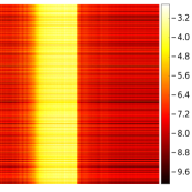
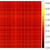
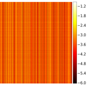
Often in our experiments, we observe common statistical attributes that could be exploited by SM3. Specifically, we see that certain entries of the stochastic gradients have (on average) similar values, and exhibit what we refer to as an activation pattern. For example, in gradients of embedding layers of deep networks, an entire row (or column) is either zero or non-zero. Similarly, in intermediate layers we often observe that gradients associated with the same unit are of similar order of magnitude. In these cases, a similar phenomenon is observed in the second-order statistics maintained by adaptive methods. In Figure 1 we visualize this phenomenon for different layers of a Transformer network. In Section B.3 we give additional illustrations of similar phenomena in convolutional layers of image classification models.

(a) Input embedding	(b) Attention layer	(c) Output softmax

Figure 1: Visualization of Adagrad’s statistics (cf. Eq. 1) for different weight matrices in Transformer-Big model trained with Adagrad on WMT’14 en$\to$fr (color intensities are in log scale).

Choice of covers.

The intuitive notion of an activation pattern motivates a natural and generic choice for the cover used by SM3 in practice. For the parameters of deep networks, that are organized as a collection of tensors, we form a cover consisting of slices of co-dimension $1$ for each tensor. Thus, for an $m\times n$ parameter matrix, the cover consists of rows and columns of the matrix. The memory requirements therefore drop from $\Theta(mn)$ to merely $\Theta(m+n)$. For a parameter tensor of dimension $n_{1}\times\cdots\times n_{p}$, the reduction in memory consumption is even more pronounced, dropping from $\Theta(\prod_{i=1}^{p}n_{i})$ to $\Theta(\sum_{i=1}^{p}n_{i})$. This virtually eliminates the memory overhead associated with maintaining the adaptive learning rates.

We argue, though only informally, that when choice of cover used by SM3 is compatible with the observed activation patterns, we expect the convergence of SM3 to be significantly better, and closely match Adagrad. Quantitatively, if each parameter $i\in[d]$ is covered by a set $S_{r}$ such that $g_{s}(j)\approx g_{s}(i)$ for all $j\in S_{r}$, then $\max_{j\in S_{r}}g_{s}^{2}(j)\approx g_{s}^{2}(i)$, and thus $\min_{r:S_{r}\ni i}\sum_{s}\max_{j\in S_{r}}g_{s}^{2}(j)\approx\sum_{s}g_{s}^{2}(i)~{}.$ Thus, the bounds in Proposition 1 and Eq. 2 are of similar order of magnitude. In other words, in such scenarios we inherit the convergence properties of Adagrad while using a negligible amount of memory. We remark that the activation pattern need not be fully specified in advance; in particular, SM3 is robust to whether a certain parameter is “row tied” or “column tied”, as long as both rows and columns are included in the cover.

Comparison with Adafactor.

Adafactor [21] is a very effective method for space-efficient adaptive optimization. SM3 and Adafactor differ in a number of important ways. First, Adafactor is only defined for matrix-shaped parameters while SM3 applies to tensors of arbitrary dimensions, and even more generally, to any predefined cover of the parameters. Second, Adafactor is in essence a fixed learning-rate algorithm, being a memory-constrained variation of Adam, and often requires a manually devised learning-rate schedule to ensure convergence. In contrast, SM3 adapts its learning rates in an adaptive, data-driven manner similar to Adagrad. Finally, SM3 comes with rigorous convergence guarantees in stochastic convex optimization settings.

5 Experiments

We demonstrate the practical efficacy of SM3 on several machine learning tasks using published state-of-the-art architectures. We focus on three domains: machine translation, language modeling, and image classification. We implemented SM3 as an optimizer in TensorFlow [1]; source code is publicly available at [3]. Our implementation follows the pseudocode of LABEL:alg:alg2, as it performed slightly yet consistently better than LABEL:alg:alg in our experiments (as predicted by our bounds). We use covers induced by rows and columns of matrices, and more generally, by slices of higher-order tensors (e.g., in convolutional layers represented by $4$-dimensional tensors), as described in Section 4. In addition to being compatible with the natural activation patterns, these covers facilitates efficient tensor operations available on GPUs and TPUs for computing max and min over the sets. In all experiments, we used the Cloud TPU-v2 device [12] where each core has 8GiB of memory. For more details on all of our experiments, including the values of hyperparameters used in each of them, see Appendix C.

5.1 Machine translation

We experimented with machine translation tasks on two standard datasets from WMT’14: English to French (en$\to$fr) with 36.3M sentence pairs, and English to German (en$\to$de) with 4.5M sentence pairs. We used the state-of-the-art Transformer architecture Vaswani et al. [23]. The basic version of this model has 93.3M parameters and consumes 0.36GiB memory. The larger variant (coined Transformer-Big) has 375.4M parameters (1.432GiB) and consists of 6 layers for its encoder and decoder, where each layer is composed of 1024 model dimensions, 8192 hidden dimensions, and 16 attention heads.

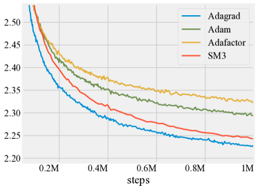
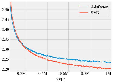
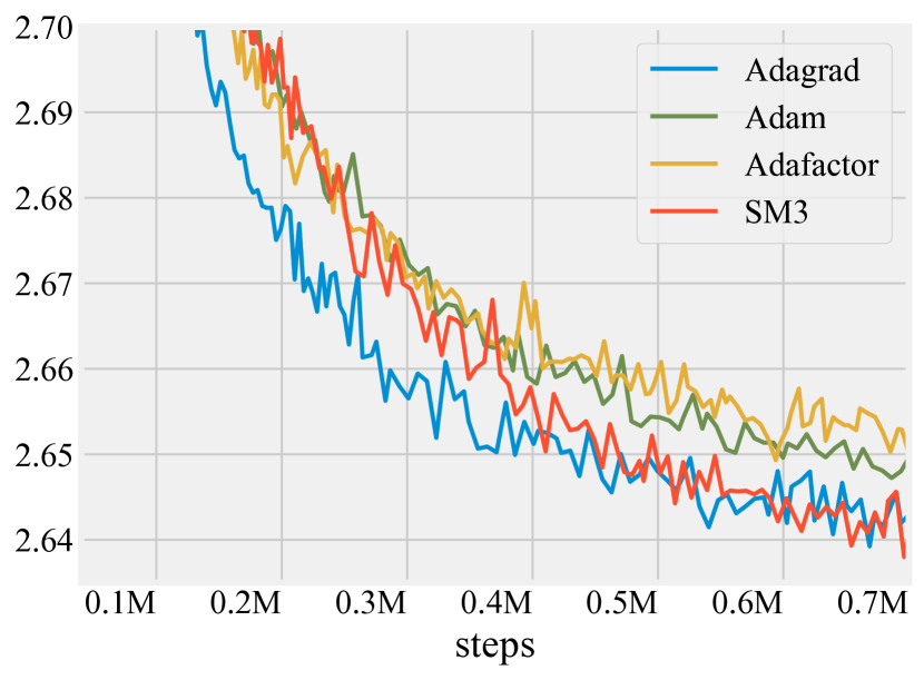
Here we report our results on the larger Transformer-Big, and defer results on the basic Transformer to Appendix B. We trained Transformer-Big on the en$\to$fr dataset with batches of size 384, and compared SM3 with several standard optimizers in each of the tasks. In all cases, we used momentum (including for Adagrad) and extensively tuned all hyperparameters. We also ran SGD with momentum (with various exponential decay schedules), but it performed poorly and hence it is omitted from the figures. The results are provided in Figure 2 and Table 1, and demonstrate that SM3 performed substantially better and provided a large improvement in BLEU score compared to Adam and Adafactor. In addition, the small memory requirements of SM3 and Adafactor allowed us to double the number of examples in a batch to a total of 768, with minimal additional computation resources. In this setting, we found that SM3 outperformed Adafactor in terms of the number of steps as well as the wall-time to convergence by roughly a factor of $2$. We further observed that SM3 approximated the Adagrad second-order statistics tightly. More details are provided in Appendix B.

Both models were trained on a $4\!\times\!4$ Cloud TPU-v2 using the Lingvo [22] sequence modeling framework, with 32K word-pieces [19] for each language pair. BLEU scores were computed on the Newstest 2014 for evaluation, on tokenized, true-case outputs, and without manual post-processing of the text, similar to [25]. Our BLEU scores are not directly comparable to those of [23]. We instead followed the experimental protocol described in a later work [6].

Figure 2: Test log-perplexity of a Transformer-Big model on WMT’14 en$\to$fr, when training with batch sizes of 384 (left) and 768 (right). For batch size of 768, Adam and Adagrad were infeasible as they exceeded the available memory.

Optimizer	Batch Size per core (total)	Memory Usage per core	BLEU
Adam	12 (384)	6.88 GiB	$38.96\pm 0.002$
Adagrad	12 (384)	6.85 GiB	$39.90\pm 0.003$
Adafactor	12 (384)	5.43 GiB	$37.89\pm 0.002$
SM3	12 (384)	5.36 GiB	$39.81\pm 0.002$
Adafactor	24 (768)	7.04 GiB	39.65 $\pm$ 0.002
SM3	24 (768)	7.02 GiB	$\bm{40.50\pm 0.001}$

Table 1: BLEU scores and memory usage for various batch sizes on the WMT’14 en$\to$fr dataset.

5.2 Language modeling

Next, we considered a language modeling task on the concatenation of Wikipedia and BooksCorpus [26], with 2.5B and 800M words respectively. We used the recent Bidrectional Encoder Representation (BERT) architecture of Devlin et al. [8], focusing on its larger variant, coined BERT-Large. BERT-Large is a large bidirectional transformer model containing 24 transformer blocks with 1024 hidden dimensions and 16 self attention heads. It has 340M parameters (1.297 GiB), and is set up to jointly optimize two objectives: (a) masked language model (Masked-LM) loss where the task is to predict masked tokens based on surrounding context, and (b) next sentence prediction (NSP) loss where the task is to predict whether two given sentences are consecutive in the text.

Figure 3: Masked LM test accuracy (left), and number of steps to get $70\%$ test accuracy as a function of the batch size (right), of the BERT-Large language model trained on Wikipedia+BooksCorpus. SM3 with batch size 2048 uses about the same amount of memory as Adam/Adagrad with batch size 1024, and scales linearly up to a batch size of $2^{16}$, at which point we hit the hardware memory limits.

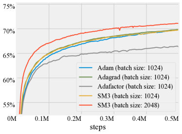
As before, we compared SM3 with Adagrad, Adam and Adafactor. Our results are presented in Figure 3. We see that SM3 worked as well as Adam and Adagrad for a fixed batch size. However, the savings in memory allowed us to train SM3 with double the batch size, resulting in a substantial increase in accuracy. The experiments were run using the open sourced code from [8] on a $8\!\times\!8$ Cloud TPU-V2 configuration.

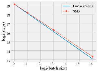
To underscore the importance of our memory savings in the context of very large models, we report additional results on the number of steps required for reaching a given solution quality for various batch sizes. We chose a solution quality of $70\%$ Masked-LM accuracy on the holdout set, which Adam and AdaGrad reached at 500k steps. We use Cloud TPU-v3 device which has 16Gib per core for this experiment. We measured the number of steps SM3 needed to reach this accuracy as a function of the batch size. Our results are presented in Figure 3. SM3 scaled almost linearly with the batch size, up to a size of $2^{16}$, at which point the training program reached the limits of memory available on hardware. We also found that SM3 came out ahead in terms of wall-time: with the same batch size, a step of SM3 was faster than Adam’s by 3%, and doubling the batch size allowed it to reach the same solution quality in almost 35% less wall-time for the same computational budget.

Optimizer	Batch Size per core (total)	Memory Usage per core
Adam	8 (1024)	6.15 GiB
SM3	8 (1024)	4.90 GiB
SM3	16 (2048)	6.02 GiB

Table 2: Training memory consumption at different batch sizes for BERT-Large on 8x8 TPUs.

5.3 AmoebaNet-D on ImageNet

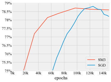
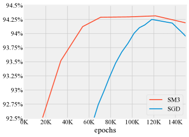
Finally, we report results from a different domain: image classification on ImageNet [18] with the state-of-the-art AmoebaNet-D architecture [16], that has recently won the Stanford DAWNBench competition [7]. We compared SM3 with SGD with momentum (Adam performed poorly on this task). The results shown in Figure 4 indicate that SM3 performed very well in this task and achieved improved convergence to state-of-the-art performance, achieving $78.71\%$ top-1 and $94.31\%$ top-5 test accuracies.

Figure 4: Top-1 (left) and Top-5 (right) test accuracy of AmoebaNet-D on ImageNet.

6 Summary

Motivated by the large increase in models sizes and the huge amounts of memory required for training them, we have presented a new memory-efficient adaptive optimization algorithm for stochastic optimization called SM3. We demonstrated empirically that SM3 can be used effectively in training modern mammoth-sized models and dramatically decrease memory overhead. Utilizing the freed memory for increasing the batch size, our experiments indicate that this saving can also lead to significant improvements in performance. Our theoretical investigation focused on convex objectives. As with many other optimization scenarios, we believe the analysis of convex memory-efficient adaptive optimization could serve as a basis for understanding non-convex settings.

Our memory savings virtually eliminate the overhead coming from the second-order statistics $\gamma_{t}$ with little and often no impact on convergence. Additional and potentially substantial improvements in memory consumption could come from compressing or sketching the momentum terms employed by virtually all first-order optimizers used in practice. We leave the exploration of this promising direction for future work.

Appendix A Omitted Proofs

A.1 Proof of 2

Proof.

Monotonicity is immediate as for any $r\in[k]$ the variable $\mu_{t}(r)$ is increasing in $t$ by definition. Therefore, $\nu_{t}(i)=\min_{r:S_{r}\ni i}\mu_{t}(r)$ is also increasing for all $i\in[d]$.

Next, since $g_{s}^{2}(i)\leq\max_{j\in S}g_{s}^{2}(j)$ for any set $S$ that contains $i$, we have

$$g_{s}^{2}(i)\leq\min_{r:S_{r}\ni i}\max_{j\in S_{r}}g_{s}^{2}(j).$$

Hence,

$$\sum_{s=1}^{t}g_{s}^{2}(i)\leq\sum_{s=1}^{t}\min_{r:S_{r}\ni i}\max_{j\in S_{r}}g_{s}^{2}(j)\leq\min_{r:S_{r}\ni i}\sum_{s=1}^{t}\max_{j\in S_{r}}g_{s}^{2}(j)=\min_{r:S_{r}\ni i}\mu_{t}(r)~{}.$$

The claim now follows since $\min_{r:S_{r}\ni i}\mu_{t}(r)=\nu_{t}(i)$. ∎

A.2 Proof of Proposition 3

Proof.

First, in order to establish monotonicity note that the algorithm maintains $\mu^{\prime}_{t}(r)=\max_{j\in S_{r}}\nu^{\prime}_{t}(j)$ for $t\geq 1$ and $r\in[k]$. Hence, for $t\geq 1$ and $i\in[d]$ we have

$$\nu^{\prime}_{t+1}(i)=\min_{r:S_{r}\ni i}\max_{j\in S_{r}}\nu^{\prime}_{t}(j)+g^{2}_{t+1}(i)\geq\nu^{\prime}_{t}(i)~{}.$$

Let $\gamma_{t}(i)=\sum_{s=1}^{t}g^{2}_{s}(i)$. We next prove by induction that $\gamma_{t}(i)\leq\nu^{\prime}_{t}(i)\leq\nu_{t}(i)$ for all $t$ and $i\in[d]$. For $t=1$ this is true as $\nu^{\prime}_{1}(i)=\gamma_{1}(i)=g^{2}_{1}(i)\leq\nu_{1}(i)$ for all $i$ by 2. For the induction step, assume that $\gamma_{t}(i)\leq\nu^{\prime}_{t}(i)\leq\nu_{t}(i)$ for all $i$ and write

$$\nu^{\prime}_{t+1}(i) =\min_{r:S_{r}\ni i}\max_{j\in S_{r}}\nu^{\prime}_{t}(j)+g^{2}_{t+1}(i)$$

$$\geq\nu^{\prime}_{t}(i)+g^{2}_{t+1}(i)$$

$$\geq\gamma_{t}(i)+g^{2}_{t+1}(i)$$

$$=\gamma_{t+1}(i)~{}.$$

On the other hand, we have

$$\nu^{\prime}_{t+1}(i) =\min_{r:S_{r}\ni i}\max_{j\in S_{r}}\nu^{\prime}_{t}(j)+g^{2}_{t+1}(i)$$

$$\leq\min_{r:S_{r}\ni i}\max_{j\in S_{r}}\nu_{t}(j)+g^{2}_{t+1}(i)$$

$$\leq\min_{r:S_{r}\ni i}\max_{j\in S_{r}}\nu_{t}(j)+\min_{r:S_{r}\ni i}\max_{j\in S_{r}}g^{2}_{t+1}(j)$$

$$\leq\min_{r:S_{r}\ni i}\mathopen{}\Big{(}\max_{j\in S_{r}}\nu_{t}(j)+\max_{j\in S_{r}}g^{2}_{t+1}(j)\Big{)}$$

$$\leq\min_{r:S_{r}\ni i}\sum_{s=1}^{t+1}\max_{j\in S_{r}}g^{2}_{s}(j)$$

$$=\nu_{t+1}(i)~{},$$

where the final inequality follows from the fact that, for all $j\in S_{r}$ one get,

$$\nu_{t}(j)=\min_{r^{\prime}:S_{r^{\prime}}\ni j}\sum_{s=1}^{t}\max_{j^{\prime}\in S_{r^{\prime}}}g^{2}_{s}(j^{\prime})\leq\sum_{s=1}^{t}\max_{j^{\prime}\in S_{r}}g^{2}_{s}(j^{\prime}).$$

Appendix B More Experiments

B.1 Tightness of SM3 approximation

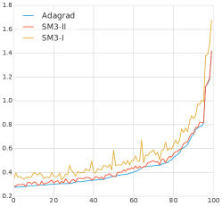
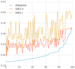
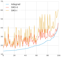
We corroborate our discussion from Section 4 with an illustration for both variants of SM3, of the tightness of approximation of Adagrad’s second-order statistics. Figure 5 demonstrates that overall SM3 provides a tight approximation, with the SM3-II performing significantly better than SM3-I, especially for higher-magnitude values.

(a) Input embedding	(b) Attention layer	(c) Output softmax

Figure 5: The magnitude of the 100 largest accumulators Eq. 1 of Adagrad for the embedding layer of a Transformer model trained on the WMT’14 en$\to$fr dataset. The accumulators are sorted by magnitude.

B.2 Results for basic Transformer on WMT’14 en$\to$de

In Figure 6 we report results for the basic Transformer after training for 700,000 steps on en$\to$de with a batch size of 1536. As in previously discussed experiments, SGD with momentum performs poorly compared to adaptive optimizers and hence is not included in the comparison.

Optimizer	Batch Size p/core (total)	BLEU
Adam	48 (1536)	27.15 $\pm$ 0.002
Adagrad	48 (1536)	27.42 $\pm$ 0.001
Adafactor	48 (1536)	26.88 $\pm$ 0.002
SM3	48 (1536)	27.32 $\pm$ 0.002

Figure 6: Test log-perplexity (left) and BLUE scores (right) on of a Transformer model trained on the WMT’14 en$\to$de dataset.

B.3 Activation patterns in convolutional networks

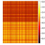
We give additional evidence of self-formation of row and column activation patterns which arise in convolutional image recognition models. See Figure 7 for an illustration.

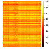(a) Filter of 7x1x256x256 convolution	(b) Output softmax

Figure 7: Visualization of gradient square statistics Eq. 1 for different weight matrices using a AmoebaNet-D model. (Color intensities are in log scale.)

Appendix C Details of Experiments

We report the settings of hyperparameters used in our experiments in Table 3. We performed a grid search on the following hyper-parameters: $\eta\in[10^{-5},10^{0}]$, $\beta_{1}\in\{0.9,0.95,0.99\}$, and $\beta_{2}\in[0.9,0.999]$ for each of the optimizers when applicable. We were able to discard a large fraction of the search space for learning rates, as large values typically cause instability and lower values make the progress slow. We found we found $\beta_{1}=0.9$ to work well for almost all experiments (where batch size < 2048) except in the case of SM3 on BERT-Large where $\beta_{1}=0.95$ worked best for $2^{13}$ and $2^{16}$ batch sizes.

Experiment	Optimizer	Batch size	Hyperparameters	Warmup ($T_{0}$)
Transformer en$\to$de	Adafactor	1536	$\eta=0.0003$, $\beta_{1}=0.9$, $\beta_{2}=0.98$	10k
	Adam	1536	$\eta=0.0004$, $\beta_{1}=0.9$, $\beta_{2}=0.98$	10k
	Adagrad	1536	$\eta=0.1$, $\beta_{1}=0.9$	10k
	SM3	1536	$\eta=0.225$, $\beta_{1}=0.9$	10k
Transformer en$\to$fr	Adafactor	384	$\eta=0.00045$, $\beta_{1}=0.9$, $\beta_{2}=0.98$	40k
	Adam	384	$\eta=0.00015$, $\beta_{1}=0.9$, $\beta_{2}=0.98$	40k
	Adagrad	384	$\eta=0.075$, $\beta_{1}=0.9$	40k
	SM3	384	$\eta=0.125$, $\beta_{1}=0.9$	40k
	Adafactor	768	$\eta=0.00045$, $\beta_{1}=0.9$, $\beta_{2}=0.98$	40k
	SM3	768	$\eta=0.25$, $\beta_{1}=0.9$	40k
BERT–Large	Adafactor	1024	$\eta=0.005$, $\beta_{1}=0.9$, $\beta_{2}=0.999$	10k
	Adam	1024	$\eta=0.0001$, $\beta_{1}=0.9$, $\beta_{2}=0.999$	10k
	Adagrad	1024	$\eta=0.25$, $\beta_{1}=0.9$	10k
	SM3	1024	$\eta=0.1$, $\beta_{1}=0.9$	10k
	SM3	2048	$\eta=0.1$, $\beta_{1}=0.9$	10k
	SM3	8192	$\eta=0.05$, $\beta_{1}=0.95$	2k
	SM3	65536	$\eta=0.15$, $\beta_{1}=0.95$	2k
AmoebaNet	SGD	4096	$\eta=6.15$, $\eta_{0}=0.042$, $\tau$=4.5k, $\beta_{1}=0.9$	1.2k
	SM3	4096	$\eta=0.5$, $\beta_{1}=0.9$	1.2k

Table 3: Hyperparameter setup used in our experiments.

We also employed a short initial “warmup” stage for all optimizers. During warmup we gradually increased the learning rate $\eta$ from zero to its maximal value during the first few thousand updates. This is a common heuristic in training of deep models, where often a high learning rate setting in the early stages of optimization causes instabilities and results in failure to converge, colloquially called “blowup”. The choice of the number of steps used for warmup does not affect the eventual performance of the trained models, and was chosen somewhat liberally before tuning the rest of the hyperparameters. We would like to stress that in each experiment, we used the same value for all optimizers. In the experiments with BERT-Large using large batch sizes, warmup was very short as experimentally it deemed almost unnecessary.

Experiment	Optimizer	LR Schedule (after warmup)	Reference
Transformer	Adam, Adafactor	$\eta\sqrt{d/t}$	[23]
BERT	Adam, Adafactor	$\eta(1-t/T)$	[8]
AmoebaNet-D	SGD (+momentum)	$\max\mathopen{}\big{\{}\eta_{0},\eta\alpha^{\lfloor t/\tau\!\rfloor}\big{\}}$	Folklore
All	Adagrad, SM3	$\eta$

Table 4: Learning rate schedules used by the algorithms we experimented with. Here, $t$ is the current time step, $\eta$ is the base learning rate, $\alpha<1$ is the decay constant, $\tau$ is the staircase step interval, $\eta_{0}$ is the minimum learning rate for staircase schedule, $T_{0}$ is the number of warmup steps, $T$ is the total number of training steps, and $d$ is the size of the model.

We note that, compared to other optimizers, SM3 has a single hyper-parameter that requires tuning, the initial learning rate $\eta$. Concretely, past the warmup phase, SM3 does not employ a schedule for learning-rate decay which is often difficult to tune. Table 4 we summarize the procedures for scheduling the learning rate of all optimizers.

For experimenting with Adafactor, we made use of the implementation in the Tensor2Tensor framework [24] and tuned the parameters as described above. We found Adafactor to work quite well on translation tasks, for which it was designed and optimized. Alas, we could not get it to work on the BERT language models. Adafactor’s implementation has numerous hyperparameters which makes it extremely difficult to set up for new domains.

References

- Abadi et al. [2016] M. Abadi, P. Barham, J. Chen, Z. Chen, A. Davis, J. Dean, M. Devin, S. Ghemawat, G. Irving, M. Isard, M. Kudlur, J. Levenberg, R. Monga, S. Moore, D. G. Murray, B. Steiner, P. Tucker, V. Vasudevan, P. Warden, M. Wicke, Y. Yu, and X. Zheng. Tensorflow: A system for large-scale machine learning. In 12th USENIX Symposium on Operating Systems Design and Implementation (OSDI 16), pages 265–283, 2016.
- Agarwal et al. [2018] N. Agarwal, B. Bullins, X. Chen, E. Hazan, K. Singh, C. Zhang, and Y. Zhang. The case for full-matrix adaptive regularization. CoRR, abs/1806.02958, 2018.
- Anil et al. [2019] R. Anil, V. Gupta, T. Koren, and Y. Singer. SM3 tensorflow optimizer. https://github.com/google-research/google-research/tree/master/sm3, 2019.
- Auer et al. [2002] P. Auer, N. Cesa-Bianchi, and C. Gentile. Adaptive and self-confident on-line learning algorithms. Journal of Computer and System Sciences, 64(1):48–75, 2002.
- Cesa-Bianchi et al. [2004] N. Cesa-Bianchi, A. Conconi, and C. Gentile. On the generalization ability of on-line learning algorithms. IEEE Transactions on Information Theory, 50(9):2050–2057, 2004.
- Chen et al. [2018] M. X. Chen, O. Firat, A. Bapna, M. Johnson, W. Macherey, G. Foster, L. Jones, M. Schuster, N. Shazeer, N. Parmar, A. Vaswani, J. Uszkoreit, L. Kaiser, Z. Chen, Y. Wu, and M. Hughes. The best of both worlds: Combining recent advances in neural machine translation. In Proceedings of the 56th Annual Meeting of the Association for Computational Linguistics, ACL 2018, pages 76–86, 2018.
- Coleman et al. [2018] C. Coleman, D. Kang, D. Narayanan, L. Nardi, T. Zhao, J. Zhang, P. Bailis, K. Olukotun, C. Re, and M. Zaharia. Analysis of dawnbench, a time-to-accuracy machine learning performance benchmark. arXiv preprint arXiv:1806.01427, 2018.
- Devlin et al. [2018] J. Devlin, M. Chang, K. Lee, and K. Toutanova. BERT: pre-training of deep bidirectional transformers for language understanding. CoRR, abs/1810.04805, 2018.
- Duchi et al. [2011] J. Duchi, E. Hazan, and Y. Singer. Adaptive subgradient methods for online learning and stochastic optimization. Journal of Machine Learning Research, 12(Jul):2121–2159, 2011.
- Gupta et al. [2018] V. Gupta, T. Koren, and Y. Singer. Shampoo: Preconditioned stochastic tensor optimization. In Proceedings of the 35th International Conference on Machine Learning, volume 80, pages 1842–1850, 2018.
- Hazan [2016] E. Hazan. Introduction to online convex optimization. Foundations and Trends in Optimization, 2(3-4):157–325, 2016.
- Jouppi et al. [2017] N. P. Jouppi, C. Young, N. Patil, D. Patterson, G. Agrawal, R. Bajwa, S. Bates, S. Bhatia, N. Boden, A. Borchers, et al. In-datacenter performance analysis of a tensor processing unit. In Computer Architecture (ISCA), 2017 ACM/IEEE 44th Annual International Symposium on, pages 1–12. IEEE, 2017.
- Kingma and Ba [2014] D. P. Kingma and J. Ba. Adam: A method for stochastic optimization. arXiv preprint arXiv:1412.6980, 2014.
- McMahan and Streeter [2010] H. B. McMahan and M. Streeter. Adaptive bound optimization for online convex optimization. COLT 2010, page 244, 2010.
- Radford et al. [2019] A. Radford, J. Wu, R. Child, D. Luan, D. Amodei, and I. Sutskever. Language models are unsupervised multitask learners. 2019.
- Real et al. [2018] E. Real, A. Aggarwal, Y. Huang, and Q. V. Le. Regularized evolution for image classifier architecture search. arXiv preprint arXiv:1802.01548, 2018.
- Reddi et al. [2018] S. J. Reddi, S. Kale, and S. Kumar. On the convergence of adam and beyond. 2018.
- Russakovsky et al. [2015] O. Russakovsky, J. Deng, H. Su, J. Krause, S. Satheesh, S. Ma, Z. Huang, A. Karpathy, A. Khosla, M. Bernstein, et al. Imagenet large scale visual recognition challenge. International Journal of Computer Vision, 115(3):211–252, 2015.
- Schuster and Nakajima [2012] M. Schuster and K. Nakajima. Japanese and korean voice search. In ICASSP, pages 5149–5152. IEEE, 2012.
- Shalev-Shwartz [2012] S. Shalev-Shwartz. Online learning and online convex optimization. Foundations and Trends in Machine Learning, 4(2):107–194, 2012.
- Shazeer and Stern [2018] N. Shazeer and M. Stern. Adafactor: Adaptive learning rates with sublinear memory cost. In Proceedings of the 35th International Conference on Machine Learning, ICML 2018, pages 4603–4611, 2018.
- [22] J. Shen, P. Nguyen, Y. Wu, Z. Chen, et al. Lingvo. https://github.com/tensorflow/lingvo.
- Vaswani et al. [2017] A. Vaswani, N. Shazeer, N. Parmar, J. Uszkoreit, L. Jones, A. N. Gomez, Ł. Kaiser, and I. Polosukhin. Attention is all you need. In Advances in Neural Information Processing Systems, pages 5998–6008, 2017.
- Vaswani et al. [2018] A. Vaswani, S. Bengio, E. Brevdo, F. Chollet, A. N. Gomez, S. Gouws, L. Jones, L. Kaiser, N. Kalchbrenner, N. Parmar, R. Sepassi, N. Shazeer, and J. Uszkoreit. Tensor2tensor for neural machine translation. CoRR, abs/1803.07416, 2018. URL http://arxiv.org/abs/1803.07416.
- Wu et al. [2016] Y. Wu, M. Schuster, Z. Chen, Q. V. Le, M. Norouzi, W. Macherey, M. Krikun, Y. Cao, Q. Gao, K. Macherey, et al. Google’s neural machine translation system: Bridging the gap between human and machine translation. arXiv preprint arXiv:1609.08144, 2016.
- Zhu et al. [2015] Y. Zhu, R. Kiros, R. Zemel, R. Salakhutdinov, R. Urtasun, A. Torralba, and S. Fidler. Aligning books and movies: Towards story-like visual explanations by watching movies and reading books. In Proceedings of the IEEE international conference on computer vision, pages 19–27, 2015.