Pan-STARRS PSF-Matching for Subtraction and Stacking

Abstract

We present the implementation and use of algorithms for matching point-spread functions (PSFs) within the Pan-STARRS Image Processing Pipeline (IPP). PSF-matching is an essential part of the IPP for the detection of supernovae and asteroids, but it is also used to homogenize the PSF of inputs to stacks, resulting in improved photometric precision compared to regular coaddition, especially in data with a high masked fraction. We report our experience in constructing and operating the image subtraction pipeline, and make recommendations about particular basis functions for contructing the PSF-matching convolution kernel, determining a suitable kernel, parallelisation and quality metrics. We introduce a method for reliably tracking the noise in an image throughout the pipeline, using the combination of a variance map and a “covariance pseudo-matrix”. We demonstrate these algorithms with examples from both simulations and actual data from the Pan-STARRS 1 telescope.

1 Introduction

The past three decades have seen the increasing importance of time-domain surveys in astronomy. These include asteroid searches such as the Lincoln Near-Earth Asteroid Research (LINEAR Stokes et al., 2000), the Lowell Observatory Near-Earth Object Search (LONEOS, Bowell et al., 1995), the Catalina Sky Survey (Larson et al., 2003), and ATLAS (Tonry et al., 2018); microlensing surveys such as MACHO (Alcock et al., 1993) and Optical Gravitational Lens Experiment (OGLE, Udalski et al., 1992); and searches for supernovae and other transient sources such as ASAS-SN (Shappee et al., 2014), the Palomar Transient Factory (PTF, Law et al., 2009), and the Robotic Optical Transient Search Experiment (ROTSE-I, Akerlof et al., 2000).

The Pan-STARRS Observatory (Chambers et al., 2017) has been a leader in the searches for both explosive transient / supernova and potentially hazardous asteroids. According to the statistics maintained by David Bishop, since 2009, 40% of all supernova have been discovered by Pan-STARRS 1. Similarly, 24% of all Near Earth Objects (NEOs) discovered to date have been found by Pan-STARRS. Since 2014, when Pan-STARRS shifted its primary mission to the search for NEOs, this fraction has increased to 41%. Both of these search programs use nightly observations to hunt for features which have changed, either between multiple images in a single night or between the current image and an archival reference image.

PSF-matched image differencing provides a useful means of identifying such variable and transient sources, especially those superimposed on complex backgrounds such as the Milky Way Bulge, or other galaxies. Because images from ground-based (and, to a lesser extent, space-based) telescopes suffer from a variable point-spread function (PSF), mere cross-correlation of catalogs cannot match the power of PSF-matched image differencing to find variable sources that are faint or blended with other objects.

Alard & Lupton (1998) first proposed a fast algorithm to solve for a convolution kernel that, when applied to an image, matches its PSF to another image. Though various features have been added to this algorithm, it is still at the heart of most image subtraction codes today. The key to the speed of the algorithm lies in the expression of the convolution kernel as a linear combination of basis functions, which allows the least-squares problem to be reduced to a matrix equation. Alard (2000) showed how this can be expanded to allow spatial variation of the kernel across the images. Of course, the basis functions used for the kernel may be completely arbitrary. These authors advocated using a set of Gaussians multiplied by polynomials; Bramich (2008) suggests using a set of discrete functions. We have tried this and other possibilities, and we will make our own suggestions for basis functions later.

Yuan & Akerlof (2008) expanded upon the original formulation of Alard & Lupton to allow for the convolution of both images to a common PSF. This technique provides additional flexibility required for good subtractions when the images are elongated in orthogonal directions, such as might be produced from optical distortions or observing at high airmass. It also removes the sometimes difficult choice of which image should be convolved to match the other (without deconvolving).

In this paper, we outline the use of PSF-matching in the Image Processing Pipeline (IPP) developed for the Pan-STARRS project. First, we introduce our formulation of the problem, built upon the above contributions (§2). Then we discuss our implementation along with lessons learned in the development of our PSF-matching code and its application to image subtraction (§3). Next, we introduce a noise model which can accurately track the noise in an image through all stages of the pipeline (§4). We introduce an application of PSF-matching to image stacking (§5) before bringing everything together with an example SN detection (§6).

2 Formulation

Given two images, $I_{1}(x,y)$ and $I_{2}(x,y)$, we desire to solve for convolution kernels, $K_{1}(u,v)$ and $K_{2}(u,v)$, such that

$$K_{1}(u,v)\otimes I_{1}(x,y)+K_{2}(u,v)\otimes I_{2}(x,y)+f(x,y)=0$$ (1)

where $f(x,y)$ is a smooth function to match the backgrounds. Following Alard & Lupton (1998), we will write the background-matching function as a linear combination of basis functions, $f_{i}(x,y)$, and each kernel as a linear combination of basis functions, $g_{i}(x,y)k_{i}(u,v)$, where the inclusion of $g_{i}(x,y)$ allows for spatial variation of the kernel. In order to enforce conservation of flux (following Alard, 2000), we specify that all of the kernel basis functions have zero sum, $\sum_{u,v}k_{i}(u,v)=0\ \forall i$. This may be achieved by scaling and subtracting one of the other kernel basis functions or simply the central element, $\delta(u,v)$ where $\delta$ is the discretised Dirac delta function in two dimensions, from each of the kernel basis functions that have non-zero sum. Then, dropping the function variables for brevity, we seek to minimise:

$$\chi^{2}=\sum_{x,y}\left(b_{0}I_{1}+\sum_{i}b_{i}g_{i}k_{i}\otimes I_{1}+\sum_{i}c_{i}g_{i}k_{i}\otimes I_{2}+\sum_{i}d_{i}f_{i}-I_{2}\right)^{2}/\sigma^{2}+\sum_{i}b_{i}^{2}p_{i}+\sum_{i}c_{i}^{2}p_{i}$$ (2)

Here, the $b_{i}$, $c_{i}$ and $d_{i}$ are the coefficients that will match the PSFs, and the $p_{i}$ are penalty functions for minimising the size of the common PSF. These penalty functions are necessary in the presence of noise, since otherwise there would be little difference in $\chi^{2}$ between wide and narrow kernels. Setting $c_{i}\equiv 0$ and $p_{i}\equiv 0$ reduces the above equation to the Alard (2000) formalism, but with the normalisation ($b_{0}$) included explicitly. In practise, the above sum will only be over small regions (known as “stamps”), and if we assume that the spatial variation is not large, then we can simply use the coordinates of the stamp centres for the $g_{i}(x,y)$; this allows a faster calculation (Alard, 2000).

To simplify the equation, we write

$$\chi^{2}=\sum_{x,y}\left(\sum_{i}a_{i}A_{i}(x,y)-I_{2}(x,y)\right)^{2}/\sigma(x,y)^{2}+\sum_{i}a_{i}^{2}P_{i}$$ (3)

where we have concatenated the vectors:

$$\begin{array}[]{lcrcccccccl}\vec{a}&=&(&b_{0}&b_{i}&\ldots&c_{i}&\ldots&d_{i}&\ldots&)\\ \vec{A}(x,y)&=&(&I_{1}&g_{i}k_{i}\otimes I_{1}&\ldots&g_{i}k_{i}\otimes I_{2}&\ldots&f_{i}&\ldots&)\\ \vec{P}&=&(&0&p_{i}&\ldots&p_{i}&\ldots&0&\ldots&)\\ \end{array}$$ (4)

Minimising $\chi^{2}$ reduces to the matrix equation, $M\vec{a}=\vec{v}$, where

$$M_{ij} = \sum_{x,y}A_{i}(x,y)A_{j}(x,y)/\sigma(x,y)^{2}+P_{i}\delta_{ij}$$ (5)

$$v_{i} = \sum_{x,y}A_{i}(x,y)I_{2}(x,y)/\sigma(x,y)^{2}$$ (6)

Here $\delta_{ij}$ is the Kronecker delta. Once this equation has been solved using regular matrix methods, the convolution kernels and background matching function may be easily calculated and applied. Note that, with the above formulation, the convolution kernel to be applied to $I_{2}$ so that the two convolved images may be subtracted is $K_{2}(u,v)=\delta(u,v)-\sum_{i}c_{i}g_{i}k_{i}$.

Up until now, we have been restricting ourselves to a very general formulation. We now point out some specific choices to be made. Adopting $x^{\ell}y^{m}$ (i.e., ordinary polynomial) or a Chebyshev or other special polynomial for the $f_{i}(x,y)$ and $g_{i}(x,y)$ is simple and convenient. The kernel basis function sets of Alard & Lupton (1998) and Alard (2000) are

$$g_{i}(x,y)k_{i}^{\prime}(u,v)=\psi_{i}x^{\ell}y^{m}u^{p}v^{q}\exp((u^{2}+v^{2})/2s_{i}^{2})$$ (7)

for integer values of $\ell,m,p,q$, and where the $\psi_{i}$ is a normalisation constant, $s_{i}$ is a Gaussian width, and the prime on $k_{i}$ indicates that it has not been normalised to zero sum (contrary to the above requirements, but shown like this for simplicity). Bramich (2008)’s choice of kernel basis functions is

$$g_{i}(x,y)k_{i}^{\prime}(u,v)=\delta(u-\ell,v-m)$$ (8)

(where spatial variation is implemented by applying this separately to discrete areas). Other basis functions are possible, and we will elaborate on these and some others we have tried in the next section.

Following Yuan & Akerlof (2008), we use as the penalty function

$$P_{i}=\Phi\sum_{u,v}(u^{2}+v^{2})^{2}k_{i}(u,v)^{2}$$ (9)

where $\Phi$ is chosen so that the $P_{i}$ have a contribution to the $A_{ii}$ that is neither negligible nor dominant (so that the equation is permitted to feel the force of the penalty, without being overwhelmed).

3 Implementation

Our implementation of PSF-matching is in the psModules library, which is wrapped by the ppSub program. Both are contained within the IPP software tree.

3.1 Kernel Basis Functions

The fact that the equations for PSF-matching can be written in a general manner (i.e., the choice of a different kernel basis set is not a different algorithm, but only a different functional choice) indicates that it is not difficult to code a system that will allow multiple basis functions. We have implemented a number of kernel basis function sets in psModules in an attempt to improve the quality of image subtractions. In the course of this, we have determined the following qualities to be desirable:

1. Generally smooth. If the basis functions have significant high-frequency power, the final convolution kernel(s) may introduce excess noise into the image. This is especially important in the outer part of the kernel, since this region is not as well constrained as the inner parts by the stamps.

2. Trending to zero. A basis function that is not trending to zero at the edges introduces a discontinuity which will result in additional noise and/or artifacts in the image (e.g., a ring around a point source).

3. Span the space. If a linear combination of the basis functions cannot reproduce the actual kernel(s) required for matching the two PSFs, then the subtraction will produce systematic residuals.

4. Small number of parameters. A large number of parameters increases the cost of computation and adds to the possibility of introducing extra noise.

The POIS kernel basis functions in psModules are equivalent to the $\delta$-functions advocated by Bramich (2008). Despite their tremendous flexibility (quality #3), these basis functions fail the other three desirable qualities. In particular, they are at the extreme opposite end of the spectrum of smoothness, and the number of parameters required for a kernel to match images with rather different PSF widths becomes prohibitive. In an attempt to redeem the notion of discrete basis functions that completely span the space without the need to specify additional parameters, we attempted binning the convolution kernel, so that the basis functions were composed of multiple clustered $\delta$-functions, with the number within a cluster growing with distance from the centre. We found that this reduced the flexibility, while failing to address the issue of smoothness. Binning radially (using rings, as opposed to blocks) suffered the same problems.

We have therefore been driven back to the classical ISIS kernel basis functions introduced by Alard & Lupton (1998). These satisfy all of the above qualities except for spanning the space. However, we have found that, with a suitable choice of Gaussian widths and by scaling these widths appropriately, we find that the ISIS kernels are quite flexible. In particular, a Gaussian of narrow width (e.g., FWHM $\sim 2$ pixels) is very effective at producing the required structure in the centre of the kernel, especially when combined with a moderately high polynomial order, while wider Gaussians do a good job of modelling the ‘skirt’, before trending to zero. Our current recommended prescription for ISIS kernels are three Gaussians, with FWHM of 2.9, 4.8 and 8.2 pixels and (ordinary) polynomial orders of 4, 2 and 2 respectively. Following advice from A. Rest (priv. comm.), we linearly scale these by the maximum FWHM of the inputs (attempts to scale by the square root of the difference of the squares, as might be naively expected, were not as effective). Our prescription is appropriate for a maximum FWHM of 9 pixels, and we set a minimum scale of 0.7 (to avoid too small a Gaussian width, which can lead to high frequency noise) and a maximum scale of 1.2 (to avoid too large a kernel, which increases computation cost and makes it more difficult to find stamps in images with a large masked fraction).

3.2 Normalisation

We have found that the most important parameter to measure accurately is the normalisation between the two images, $b_{0}$ in the above formulation. Because the other kernel basis functions have zero sum, an error in the normalisation cannot be compensated by tweaking the other coefficients. Nevertheless, through the least-squares solution, the coefficients of what would normally be even functions (without the zero sum) are adjusted to minimise the $\chi^{2}$ in an attempt to compensate, resulting in strong ring-like residuals.

In order to accurately measure the normalisation without the interference of the convolution kernels, we solve for $b_{0}$ and a constant background differential term ($d_{0}$) separately from the other parameters. We may do this because the normalisation and background differential are the only terms that add flux to the image; the other terms just move the flux around. Taking a lesson from PSF-fitting photometry, we specifically do not weight by the variance in the matrix accumulations, i.e., we set $\sigma(x,y)\equiv 1$. This is because the smaller Poisson noise of brighter pixels would bias the normalisation too high.

3.3 Stamps

Since we restrict the analysis of the kernel required for PSF matching to the small “stamps” centered on bright stars, the choice of stamps is key to successful PSF-matching. The convolution kernel is only as good as the stamps used to construct it. We use a merged list of sources from photometry of the two input images as the basis of our stamps list. Sources with a flag indicating that it is anything other than a pristine astrophysical source are excluded. At the present time, we make no effort to select sources of a particular color or range of colors.

We exclude sources with any masked pixels that would affect the calculation of the convolution kernel. For a camera such as Pan-STARRS 1’s Giga-Pixel Camera 1 (GPC1) with a high ($\sim 20\%$) masked fraction and where these masked pixels are widely distributed, this can make it difficult to find sufficient high-quality stamps. To minimise this, we try to keep the size of the convolution kernel small.

We divide the image into subregions of size typically about 1 arcmin². The source with the brightest peak pixel over a defined threshold (e.g., $5\sigma$ above background) within each subregion (if any) is nominated as a stamp center. The use of these subregions ensures the stamps are distributed over the entire image.

We do not explicitly discriminate against galaxies as stamps (they can provide information on the convolution kernel, though not as effectively as point sources), except that stars will typically be chosen first within a subregion because of their higher surface brightness.

Discrepant stamps are removed (and replaced, if possible) using multiple solution iterations.

3.4 Masking

Masked pixels (e.g., due to saturation, artifacts, etc.) do not contribute to the convolution. To minimise the effect these pixels have on the convolved image(s), we adopt a distinction between “bad” pixels and “poor” pixels first suggested by A. Becker and implemented in the HOTPANTS code. Pixels in a convolved image that are seriously affected by the presence of a masked pixel in the original image are flagged as CONV.BAD, while pixels that may only be slightly affected are flagged as CONV.POOR. The (box) radius of the distinction between the two is chosen to be the radius at which the sum of the square of the kernel drops below a chosen fraction (currently the default is 0.2) of the total.

3.5 Optimisations and parallelisation

Parallelisation is becoming increasingly important as practical limits to shrinking sizes and increasing clock rates set in, and the CPU industry turns to multiple core architectures for increasing computational power. Fortunately, the two major stages of the PSF-matching process may be easily parallelised.

The first major stage of the PSF-matching process is the calculation of the equation. This may be done on each of the stamps in independent threads. We calculate a least-squares matrix independently for each stamp, since these need not be recalculated for each rejection iteration. Summing these matrices and producing a solution is fairly fast and need not be threaded.

The second major stage is the application of the solution to the images. Having assumed in the construction of the least-squares equation that spatial variations of the kernels are small on the scale of a stamp, we are quite entitled to continue that assumption by dividing the image into regions about the size of a stamp and applying a single kernel to each in independent threads. We use Fast Fourier Transforms to perform the convolutions, as this is faster than a direct convolution for kernels larger than about 13 pixels (full width, square), as ours tend to be.

3.6 Quantifying quality

We calculate several quantities for the purposes of evaluating the quality of the PSF-matching process. These are stored in our processing database, allowing a quick comparison of these quantities for the multitude of images processed, and identification of poor subtractions.

For each stamp, we calculate the residual from applying the solution. In this case, we do divide through by the variance, softened by adding a scaled version of the flux, so that the brightest pixels do not exert undue influence on the fit. We use the mean of the squared residuals (effectively a $\chi^{2}$) as a measure of the quality of the stamp’s subtraction. The mean and standard deviation of these residuals over the collection the stamps serves as a measure of the quality of the subtraction over the entire image. The number of stamps used in the calculation is also recorded.

Deconvolution (narrowing a PSF instead of broadening it) is often the enemy of the PSF-matching process — when the solution for the kernel involves deconvolution, the result is usually noisy or inaccurate. We quantify the deconvolution by measuring, as a function of radius, the sum of kernel values enclosed within that radius relative to the total kernel sum. When the maximum deconvolution fraction is significantly in excess of unity, then the result is typically unacceptable. We also calculate and record the first and second moments of the kernel (realised at the center of the image, if spatially variable).

3.7 Examples

On the night of 2010 June 27 (UT), Pan-STARRS 1 (PS1) took 550 exposures (534 as part of the “3$\pi$ Survey” and 16 as part of the “Medium-Deep Survey”) which were automatically processed by the IPP. As part of this processing, 20,240 subtractions were made. Of these, 20,053 completed cleanly, while 187 were flagged as having bad quality data (2 due to insufficient unmasked area, and 185 due to failure to measure the PSF on the convolved image). In Figure 1 we show the distributions of various quality metrics.

Figure 1: Distributions of quality metrics from 20,053 subtractions. The kernel y and yy moments are similar to the x and xx moments, respectively, so we do not show them.

Based on these distributions and inspection of the subtractions, we recommend using the following cuts to flag bad subtractions:

• Number of stamps used $<$ 3

• Normalised mean deviation $>$ 0.5

• Normalised r.m.s. deviation $>$ 0.3

• First moments (x, y) of kernel $>$ 0.5

• Second moments (xx, yy) of kernel $<$ 0

• Maximum deconvolution fraction $>$ 1.03

Applying these cuts flag 132 of our subtractions (or 0.66%) as bad.

4 Noise Model

The accurate detection and measurement of astrophysical sources on images depends on a reliable noise model. The usual practise in the analysis of optical images is to assume that the noise in a processed image is Poisson ($\sigma^{2}=N+r^{2}$, where $\sigma$ is the noise in electrons, $N$ is the number of electrons recorded and $r$ is the detector read noise in electrons; the electronic gain is required to convert between data units and electrons) or to measure the noise directly from the image. Both of these practises ignore the reduction history of the image being analysed, erring in the presence of correlated noise produced by resampling and convolving, or even when there is non-uniform vignetting or dark current. This has led to some progressive software packages producing (e.g., SWarp: Bertin et al., 2002) and using (e.g., SExtractor: 1996AAS..117..393B) weight maps to characterise the noise over the image. Because of simplicity and lower calculation cost relative to weights or standard deviations, we prefer to calculate and propagate the variance as the “weight map”.

4.1 Covariance

In the presence of multiple convolutions, merely tracking the variance is insufficient to characterise the noise properties of an image. A convolution moves noise from the diagonal terms (“variance”) of the covariance matrix into the off-diagonal terms (“covariance”), so that subsequent convolutions, even if they attempt to account for the variance, will mis-estimate the noise in the twice-convolved image because the noise pushed into the covariance by the first convolution has not been accounted for in the second convolution.

Multiple convolutions are impossible to avoid for any pipeline that wishes to do anything more than photometry of an image directly from the detector. If sources are to be identified on a subtracted image, there will usually be at least one resampling/interpolation to align the images, at least one convolution to match the PSFs and then another convolution by a matched filter to identify sources — three convolutions. It is therefore important to treat the covariance.

However, it is not feasible to calculate or store a full covariance matrix. For example, a $2048\times 2048$ image (about $4\times 10^{6}$ pixels; small by modern standards) would require in excess of $10^{13}$ elements. Even if we recognise that the covariance matrix is quite sparse, the size is still prohibitive (a $6\times 6$ kernel, typical for Lanczos interpolation, applied to our hypothetical image would require in excess of $10^{8}$ elements).

Instead, we track the average covariance for an image using a “covariance pseudo-matrix” (of order a few $\times 10^{2}$ elements), combined with a variance map (same dimension as the flux image). The covariance pseudo-matrix tracks the average covariance between a single pixel and its neighbours (i.e., the off-diagonal terms of the full covariance matrix relative to the diagonal terms), while the covariance map tracks the variation of the variance across the image (i.e., the diagonal terms of the full covariance matrix). The covariance pseudo-matrix is assumed to be identical for all pixels; this isn’t strictly true because convolution kernels may vary over the image, yet it’s a reasonable and useful approximation that allows us to accurately model the noise in the image through all stages of the pipeline.

4.2 Prescription

When we apply a convolution kernel to an image, we are making a linear mapping from $m$ variables, $x_{i}$ (the flux in the unconvolved image), to $n$ variables, $y_{j}$ (the flux in the convolved image):

$$y_{j}=\sum_{i}A_{ij}x_{i}$$ (10)

If the covariance matrix for $\vec{x}$ is $M^{x}$, then the covariance matrix for $\vec{y}$ is:

$$M^{y}_{ij}=\sum_{k}\sum_{\ell}A_{ik}M^{x}_{k\ell}A_{\ell j}$$ (11)

A covariance pseudo-matrix may be thought of like a kernel (i.e., an image extending to both positive and negative offsets in both dimensions, where the central pixel corresponds to zero offset on the image to which it is applied), where the $0,0$ element is the reference for all others. To calculate an element of the covariance pseudo-matrix of the convolved image, we sum the product of all possible combinations of stepping from the element of interest to the central (reference) element via a convolution kernel ($A_{ik}$), the input covariance pseudo-matrix ($M^{x}_{k\ell}$) and another instance of the convolution kernel ($A_{\ell j}$). The output covariance pseudo-matrix therefore has dimensions of twice the size of the kernel, plus the size of the input covariance pseudo-matrix.

The calculation of the covariance pseudo-matrix, requiring three nested iterations, can become expensive. To prevent this, the input pseudo-matrix and/or kernel may be truncated by discarding the outer parts which are not strongly significant (e.g., the outer 1% of the sum of absolute values). The calculation is also easily parallelised, since each element of the pseudo-matrix may be calculated independently of the others.

When convolving, the image and variance are calculated in the usual manner:

$$I^{\prime}(x,y) = \sum_{u,v}k(u,v)I(x-u,y-v)$$ (12)

$$V^{\prime}(x,y) = \sum_{u,v}k(u,v)^{2}V(x-u,y-v)$$ (13)

where $I(x,y)$ is the (flux) image, $V(x,y)$ is the variance map, primes indicate the result of the convolution, and $k(u,v)$ is the convolution kernel. Due to the separation of the variance and covariance, there is an additional factor of $K=[\sum_{u,v}k(u,v)^{2}]^{-1}$, which may be absorbed in either the variance or covariance pseudo-matrix (since it is multiplicative).

Then, with the covariance pseudo-matrix calculated, the variance for each pixel on the (flux) image is the variance map multiplied by the reference (central) value of the covariance pseudo-matrix (the “covariance factor”). For convenience, we normally transfer the covariance factor from the pseudo-matrix into the variance map, so that analyses that do not include convolution need not bother with the covariance.

4.3 Use in practise

When using a spatially variable kernel (e.g., interpolation by anything more than a constant shift; or PSF-matching as outlined above), it is impossible for this simple model (variance map with a single covariance pseudo-matrix) to provide a perfect description of the noise properties of an image, and approximations must be made. Our usual practise is to calculate a sample of covariance pseudo-matrices over the image and take the average as representative of the entire image. Absorbing the $K$ into the variance map washes out the structure caused by the spatially variable kernel. Absorbing the $K$ into the covariance pseudo-matrix washes out changes in the covariance as a function of position, but this is necessarily the case anyway (there is only one covariance pseudo-matrix) and covariance errors are a more subtle effect than variance errors, and so this is our preference.

When applying a spatially-variable PSF-matching kernel, we apply a constant kernel to small patches. For each patch we calculate the covariance factor (not the entire covariance pseudo-matrix, which takes much longer) from the kernel and apply it to the variance of that patch. We then remove the covariance factor from the average covariance pseudo-matrix (calculated from a much smaller array of kernels, because of the expense of calculation) since it has already been applied.

Binning an image may be thought of as convolution where the kernel has a constant value, followed by a change in scale. It is important, when changing the scale of the image and variance map, that the scale of the covariance pseudo-matrix also be changed appropriately. In the case of binning with an integer scale, this is straightforward. For resampling with a non-integer scale, we use bilinear interpolation to resample the covariance pseudo-matrix. Unfortunately, this can introduce a small amount of extra power into the covariance pseudo-matrix which cannot easily be accounted for — preserving the total variance and covariance disturbs the noise model for the resampled image, while preserving the covariance factor affects the noise model for convolutions of the resampled image. In an attempt to have the best of all worlds, we choose to preserve the total covariance excluding the variance.

When adding or subtracting (flux) images, the variance maps should be summed, and the covariance pseudo-matrices combined using a weighted average, where the weights are the average variances measured from the variance maps. This is not perfectly correct for bright sources (nor can it be, given the limitations of our simple noise model), but this produces the correct noise for the background, which enables faint sources to be detected.

4.4 Example

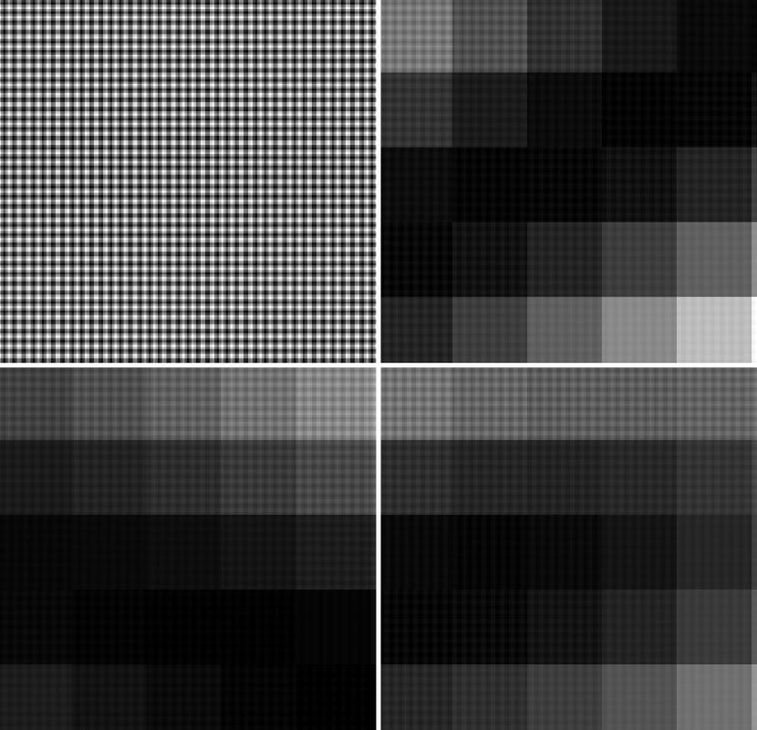
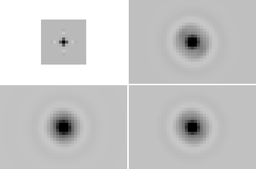
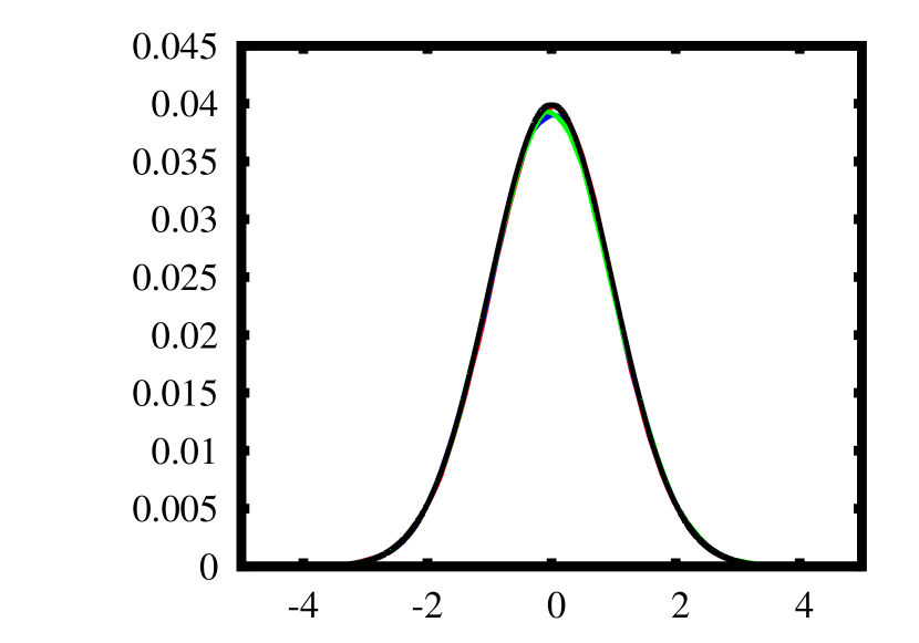
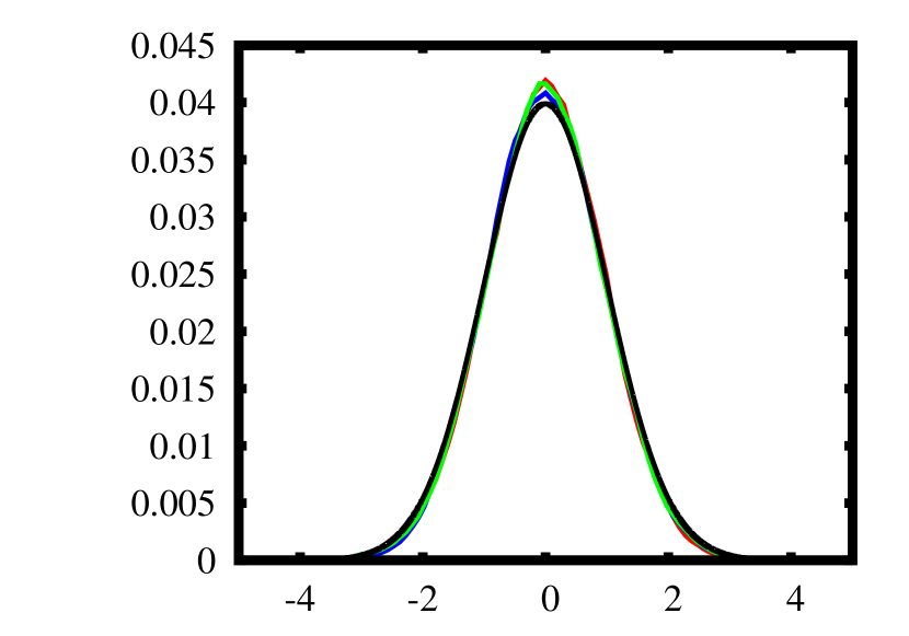
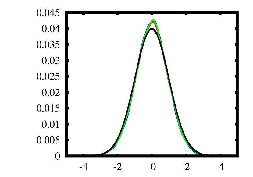
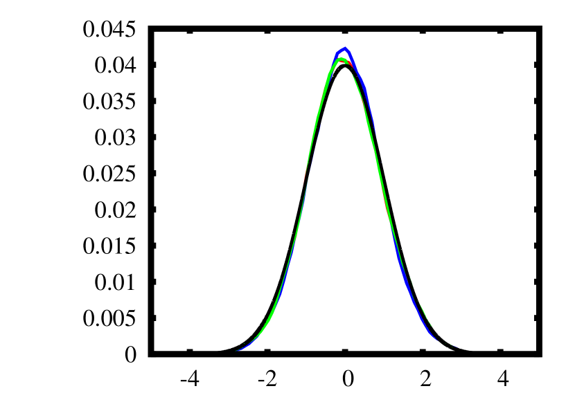
To demonstrate our noise model, we generated fake images composed entirely of Gaussian noise of different levels. We then manipulated these images in a similar manner as for real pipeline operations, tracking the variance and covariance. These operations include warping (rotation and interpolation on a finer pixel scale), convolution, subtraction of two warped, convolved images, stacking multiple warped images, subtraction of two convolved stacks, and subtraction of a convolved warped image from a convolved stacked image. Actual PSF-matching kernels were used for the convolutions. Example variance maps and covariance pseudo-matrices are shown in Figures 2 and 3. At each stage, we convolved with a Gaussian, simulating a matched filter for photometry, and measured the standard deviation of the (flux) image divided by the square-root of the epected variance, which should be unity if the noise is being properly tracked. We find that this statistic is always within 6% of unity, with a mean of 0.98 and r.m.s. of 0.03. Example histograms are shown in Figure 4.

Figure 2: Example variance maps from our simulated pipeline. The original (detector frame) variance maps are uninterestingly constant and so are not shown. Top left: Variance map after warping (rotation and scale change). The small-scale structure is due to interference between the original and new pixel scales. Top right and bottom left: Variance maps after convolving warped images with a spatially variable PSF-matching kernel. The small-scale structure from the warps is still apparent. The moderate-scale squares are due to the application of a constant kernel on scales of about $10^{2}$ pixels, while the large-scale structure comes from the spatial variation of the (PSF-matching) convolution kernel. Bottom right: Variance map after subtracting the convolved warps. While the scale and orientation for each panel is identical, the color maps are separate.

Figure 3: Covariance pseudo-matrices from our simulated pipeline. The original (detector frame) covariance pseudo-matrix consists of a single pixel of unit value and so is not shown. The panels are arranged in the same manner as Figure 2. Warping (in this case, using a LANCZOS3 interpolation kernel) introduces a small amount of covariance, but the PSF-matching convolution introduces substantially more. While the scale and orientation for each panel is identical, the color maps are separate.

Figure 4: Histograms of flux divided by the expected noise after convolving with a Gaussian (matched filter for photometry) the results of various stages of our simulated pipeline. In each panel, the black line is a Gaussian of unit width and appropriate normalisation, while the colored lines (sometimes hidden behind the black line) are different realisations from our simulated pipeline. Top left: Photometry on the original image. Top right: Photometry on a warped image. Bottom left: Photometry on a subtraction. Bottom right: Photometry on a stack.

5 Image Stacking

Image stacking is a crucial tool for synoptic surveys, since it allows long exposures to be traded for multiple visits that can be used to identify transients, simultaneously satisfying those who desire many repeated exposures (e.g., for the discovery of transients) and those who want deep exposures (“wallpaper science”). Stacking images is straightforward if the images are all taken under similar conditions, or with an idealised detector, but neither case is realistic for ground-based synoptic survey data. In the presence of masked pixels (even due to such mundane causes as gaps between devices in a mosaic) and a variable PSF, a direct combination of images (using any averaging statistic) will result in an image where the PSF is spatially variable in a discontinuous fashion, which can introduce systematic errors to photometry and shape analyses.

Since it would be expensive and unwieldy to calculate the PSF for each pixel of a stack image separately based on the contributing inputs, we instead convolve each input to a common PSF (“PSF homogenization”) using the same PSF-matching technique as for image subtraction, resulting in a stacked image where the PSF is known everywhere and may be modeled as varying continuously over the image. While this necessarily results in some lost sensitivity due to degrading images to a wider PSF, this must be balanced against the gain in sensitivity that comes from controlled systematics. In any case, it is not impractical to create stacks both with and without this convolution, or with a range of PSF widths, allowing the users to choose the most appropriate for their particular application (e.g., unconvolved stack for point source detection, convolved stack for analysis of point sources).

5.1 Method

From the known PSF models for the inputs, we determine an “envelope PSF” by realising a circular version of each PSF with a common peak flux, taking the maximum value pixel by pixel, and fitting the result with a PSF model. The envelope PSF may be allowed to vary spatially. With some more development work, we hope to be able to perform this envelope calculation directly using the PSF model parameters, and to reject inputs that would result in a net loss of signal-to-noise ratio in the stack by their inclusion (due to imposing on all other inputs a larger PSF envelope than necessary).

To homogenize the PSFs, we create a fake target image using the envelope PSF and the known positions of (point) sources in the field. This image is used as a target ($I_{2}$) for our PSF-matching code (setting $c_{i}\equiv 0$) to convolve each image to the common envelope PSF. Forcing the envelope PSF to be circular reduces the complexity of this PSF-matching process, and also when the stack is used as the input or reference for image subtraction.

Once the inputs have a common PSF, it is a simple matter to identify outlier pixels (artifacts, transients, etc.) and reject these from contributing to the stack, without having to worry about the cores of stars, etc., which may otherwise be a function of the input PSF. We flag outlier pixels on a separate mask image, to which we apply a matched filter (the convolution kernel we applied to the image) to identify bad pixels on the original image (i.e., before convolution); this ensures the entire area the bad pixel contributes on the convolved image is masked, and not just those that were sufficiently bright to trigger the rejection. The same list of bad pixels in the inputs may be used for combining images without convolution.

5.2 Examples

As a demonstration of the importance of convolution to match PSFs in the stack, we created two stacks from observations by PS1 + Giga-Pixel Camera (GPC1) of the Stellar Transit Survey (STS) field. We chose this field because of the high stellar density that will allow a good comparison of the photometry. The observations were made under reasonable conditions (both transparency and seeing) for the purpose of generating a high-quality stack to be used as the template in image differencing. The images were processed through the IPP in the standard manner (dark and flat-field corrections were applied, bad pixels flagged, photometry and astrometry measured) and the images were transformed (“warped”) to common reference frames (“skycells”). We chose a skycell for which the inputs have a large amount of overlap.

GPC1 suffers from a condition where pixels that become super-saturated on an exposure contaminate other pixels within the same column on subsequent exposures (“burn trails”). These pixels can easily be identified and are usually modeled and subtracted fairly well, but the high stellar density of the STS field affects the quality of the burn trail subtraction. We therefore masked all pixels that might contain a burn trail, but due to the high stellar density and frequent dithers, this can be a large fraction of the skycell for these images. This larger than usual masking fraction may amplify any differences between our convolved stacks and regular (unconvolved) coadditions.

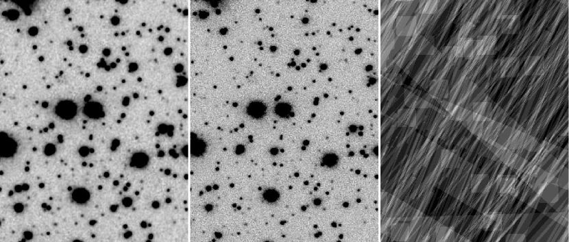
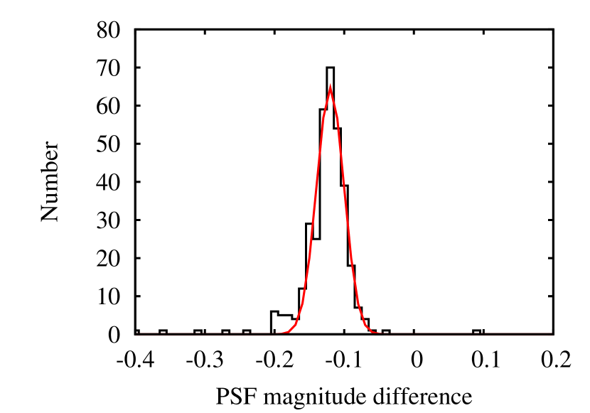
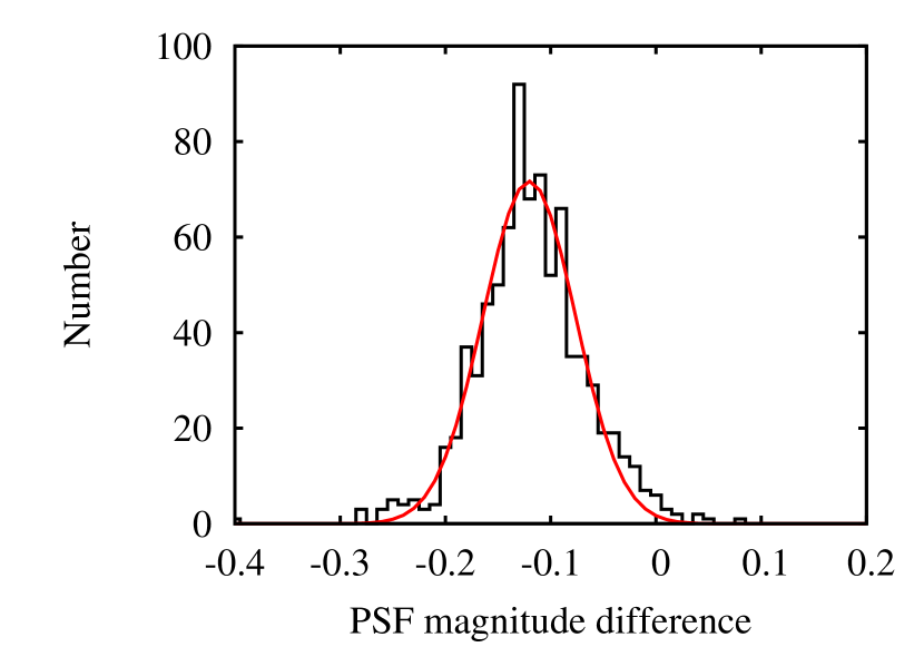
We chose two disjoint subsets of exposures, each spanning the available observing time, and stacked them using our stacking program, ppStack. This program generates a convolved stack using the above method, along with an unconvolved stack using the same pixel rejection list as for the convolved stack. In both cases, the pixels are stacked with weights for each image set to the mean variance in the convolved image. A convolved and unconvolved stack are displayed in Figure 5. We then used our photometry program, psphot, to perform PSF photometry on the two convolved and two unconvolved stacks. In Figure 6 we compare the magnitude difference as a function of magnitude between the convolved and unconvolved stacks, along with the distribution of magnitude differences. A Gaussian fit to the core of each distribution yields a width of 0.020 mag for the convolved stack and 0.044 mag for the unconvolved stack, demonstrating the need for PSF homogenisation for accurate stack photometry. Of course, the convolved stacks are not as deep as the unconvolved stacks, but one could easily imagine a hybrid photometry scheme where bright objects are measured from the convolved stack while faint objects are measured from the unconvolved stack, or detected on the unconvolved stack but measured on the convolved stack.

Figure 5: Comparison of stacked and unconvolved stacks. Left: Convolved stack. Middle: Unconvolved stack. Right: Exposure map for the convolved stack; note the fine structure due to coaddition of masked images.

Figure 6: Comparison of photometry between convolved and unconvolved stacks. Top: Difference in magnitude as a function of (instrumental) magnitude for convolved (left) and unconvolved (right) stacks. Bottom: Histogram of magnitude difference for sources with instrumental magnitude between -15 and -14 for convolved (left) and unconvolved (right) stacks. A Gaussian fit has been overplotted (red); the widths are 0.020 mag (convolved) and 0.044 mag (unconvolved).

6 Putting it all together

We are routinely running our image stacking and subtraction codes on images from the Pan-STARRS 1 telescope, from which SN discoveries are being made (e.g., see Botticella et al., 2010).

As a demonstration of the above techniques, we re-create the discovery of SN 2009kf (Botticella et al., 2010), showing each step along the way. Our input data consists of 8 $r$-band exposures of PS1 Medium-Deep field 08 (MD08) from before the discovery and 4 $r$-band exposures from the discovery epoch. The images were processed through the IPP in the standard manner and warped to skycells.

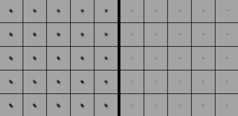
We stacked the exposures from before the discovery to use as our template. We subtracted this reference from each of the individual warps from the discovery epoch. Example PSF-matching kernels are shown in Figure 7. It is apparent that the kernels are strongly spatially variable. In this case, the second kernel ($K_{2}$) does not play a major part in the PSF-matching (because the reference stack PSF has been circularised as part of the PSF homogenisation process), but it does contain a small amount of power that helps produce a good subtraction.

Figure 7: Kernels for PSF-matching an individual exposure to the reference stack. Left: Kernel applied to the individual exposure ($K_{1}$). Right: Kernel applied to the reference stack ($K_{2}$). For each, the kernel is realised at a grid of points over the image, so that the spatial variation can be visualised.

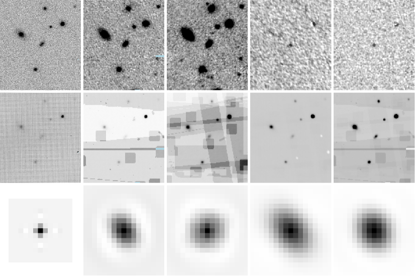
We also stacked the discovery epoch warps and subtracted from this stack the template. The SN is well-detected in all cases (Figure 8). The variance maps for the stacks are complicated due to chip gaps and the rejection of artifacts, and this structure is propagated to the subtracted images. Following subtraction, the covariance is extended by as much as FWHM $\sim$ 5 pixels, and in some cases, elongated. Because of these effects, photometry of variable sources such as SNe and asteroids that does not take into account the variance structure and covariance is likely to mis-estimate the photometric errors.

Figure 8: Recreation of the discovery of SN 2009kf (Botticella et al., 2010), demonstrating the techniques from this paper. Across a row, the images are an individual exposure, stack of the discovery epoch exposures, the reference stack, subtraction of the reference from the individual exposure, and subtraction of the reference from the discovery epoch stack. The rows are the flux (top), the variance map (middle) and the covariance pseudo-matrix (bottom). The orientation of the flux and variance maps is identical, but the color maps are not. The covariance maps are displayed at a common scale, but with different color maps. The SN is well-detected in both the individual and stack subtractions.

The algorithms presented here have been implemented within the PS1 IPP, which is freely available from our Subversion repository. The IPP has been running routinely on data collected by PS1 since February 2010, resulting in the discovery of hundreds of SNe and thousands of asteroids as PS1 surveys the heavens.

References

- Akerlof et al. (2000) Akerlof, C., Balsano, R., Barthelmy, S., Bloch, J., Butterworth, P., Casperson, D., Cline, T., Fletcher, S., Gisler, G., Hills, J., Kehoe, R., Lee, B., Marshall, S., McKay, T., Pawl, A., Priedhorsky, W., Seldomridge, N., Szymanski, J., & Wren, J. 2000, ApJ, 542, 251
- Alard (2000) Alard, C. 2000, A&AS, 144, 363
- Alard & Lupton (1998) Alard, C. & Lupton, R. H. 1998, ApJ, 503, 325
- Alcock et al. (1993) Alcock, C., Allsman, R. A., Axelrod, T. S., Bennett, D. P., Cook, K. H., Park, H. S., Marshall, S. L., Stubbs, C. W., Griest, K., Perlmutter, S., Sutherland, W., Freeman, K. C., Peterson, B. A., Quinn, P. J., & Rodgers, A. W. 1993, in Astronomical Society of the Pacific Conference Series, Vol. 43, Sky Surveys. Protostars to Protogalaxies, ed. B. T. Soifer, 291
- Bertin et al. (2002) Bertin, E., Mellier, Y., Radovich, M., Missonnier, G., Didelon, P., & Morin, B. 2002, in Astronomical Society of the Pacific Conference Series, Vol. 281, Astronomical Data Analysis Software and Systems XI, ed. D. A. Bohlender, D. Durand, & T. H. Handley, 228–+
- Botticella et al. (2010) Botticella, M. T., Trundle, C., Pastorello, A., Rodney, S., Rest, A., Gezari, S., Smartt, S. J., Narayan, G., Huber, M. E., Tonry, J. L., Young, D., Smith, K., Bresolin, F., Valenti, S., Kotak, R., Mattila, S., Kankare, E., Wood-Vasey, W. M., Riess, A., Neill, J. D., Forster, K., Martin, D. C., Stubbs, C. W., Burgett, W. S., Chambers, K. C., Dombeck, T., Flewelling, H., Grav, T., Heasley, J. N., Hodapp, K. W., Kaiser, N., Kudritzki, R., Luppino, G., Lupton, R. H., Magnier, E. A., Monet, D. G., Morgan, J. S., Onaka, P. M., Price, P. A., Rhoads, P. H., Siegmund, W. A., Sweeney, W. E., Wainscoat, R. J., Waters, C., Waterson, M. F., & Wynn-Williams, C. G. 2010, ApJ, 717, L52
- Bowell et al. (1995) Bowell, E., Koehn, B. W., Howell, S. B., Hoffman, M., & Muinonen, K. 1995, in Bulletin of the American Astronomical Society, Vol. 27, AAS/Division for Planetary Sciences Meeting Abstracts #27, 1057
- Bramich (2008) Bramich, D. M. 2008, MNRAS, 386, L77
- Chambers et al. (2017) Chambers, K. C., Magnier, E. A., Metcalfe, N., & et al. 2017, ArXiv e-prints
- Larson et al. (2003) Larson, S., Beshore, E., Hill, R., Christensen, E., McLean, D., Kolar, S., McNaught, R., & Garradd, G. 2003, in Bulletin of the American Astronomical Society, Vol. 35, AAS/Division for Planetary Sciences Meeting Abstracts #35, 982
- Law et al. (2009) Law, N. M., Kulkarni, S. R., Dekany, R. G., Ofek, E. O., Quimby, R. M., Nugent, P. E., Surace, J., Grillmair, C. C., Bloom, J. S., Kasliwal, M. M., Bildsten, L., Brown, T., Cenko, S. B., Ciardi, D., Croner, E., Djorgovski, S. G., van Eyken, J., Filippenko, A. V., Fox, D. B., Gal-Yam, A., Hale, D., Hamam, N., Helou, G., Henning, J., Howell, D. A., Jacobsen, J., Laher, R., Mattingly, S., McKenna, D., Pickles, A., Poznanski, D., Rahmer, G., Rau, A., Rosing, W., Shara, M., Smith, R., Starr, D., Sullivan, M., Velur, V., Walters, R., & Zolkower, J. 2009, PASP, 121, 1395
- Shappee et al. (2014) Shappee, B. J., Prieto, J. L., Grupe, D., Kochanek, C. S., Stanek, K. Z., De Rosa, G., Mathur, S., Zu, Y., Peterson, B. M., Pogge, R. W., Komossa, S., Im, M., Jencson, J., Holoien, T. W.-S., Basu, U., Beacom, J. F., Szczygieł, D. M., Brimacombe, J., Adams, S., Campillay, A., Choi, C., Contreras, C., Dietrich, M., Dubberley, M., Elphick, M., Foale, S., Giustini, M., Gonzalez, C., Hawkins, E., Howell, D. A., Hsiao, E. Y., Koss, M., Leighly, K. M., Morrell, N., Mudd, D., Mullins, D., Nugent, J. M., Parrent, J., Phillips, M. M., Pojmanski, G., Rosing, W., Ross, R., Sand, D., Terndrup, D. M., Valenti, S., Walker, Z., & Yoon, Y. 2014, ApJ, 788, 48
- Stokes et al. (2000) Stokes, G. H., Evans, J. B., Viggh, H. E. M., Shelly, F. C., & Pearce, E. C. 2000, Icarus, 148, 21
- Tonry et al. (2018) Tonry, J. L., Denneau, L., Heinze, A. N., Stalder, B., Smith, K. W., Smartt, S. J., Stubbs, C. W., Weiland, H. J., & Rest, A. 2018, PASP, 130, 064505
- Udalski et al. (1992) Udalski, A., Szymanski, M., Kaluzny, J., Kubiak, M., & Mateo, M. 1992, Acta Astron., 42, 253
- Yuan & Akerlof (2008) Yuan, F. & Akerlof, C. W. 2008, ApJ, 677, 808