CapsAttacks: Robust and Imperceptible Adversarial Attacks on Capsule Networks

Abstract

Capsule Networks preserve the hierarchical spatial relationships between objects, and thereby bears a potential to surpass the performance of traditional Convolutional Neural Networks (CNNs) in performing tasks like image classification. A large body of work has explored adversarial examples for CNNs, but their effectiveness on Capsule Networks has not yet been well studied. In our work, we perform an analysis to study the vulnerabilities in Capsule Networks to adversarial attacks. These perturbations, added to the test inputs, are small and imperceptible to humans, but can fool the network to mispredict. We propose a greedy algorithm to automatically generate targeted imperceptible adversarial examples in a black-box attack scenario. We show that this kind of attacks, when applied to the German Traffic Sign Recognition Benchmark (GTSRB), mislead Capsule Networks. Moreover, we apply the same kind of adversarial attacks to a 5-layer CNN and a 9-layer CNN, and analyze the outcome, compared to the Capsule Networks to study differences in their behavior.

1 Introduction

Convolutional Neural Networks (CNNs) showed a great improvement and success in many Machine Learning (ML) applications, e.g., object detection, face recognition, image classification (Bhandare et al., 2016). However, the spatial hierarchies between the objects, e.g., orientation, position and scaling, are not preserved by the convolutional layers. CNNs are specialized to identify and recognize the presence of an object as a feature, without taking into account the spatial relationships across multiple features. Recently, Sabour and Hinton et al. (2017) proposed the CapsuleNet, an advanced Neural Network architecture composed of so-called capsules, which is trained based on the Dynamic Routing algorithm between capsules. The key idea behind the CapsuleNet is called inverse graphics: when the eyes analyze an object, the spatial relationships between its parts are decoded and matched with the representation of the same object in our brain. Similarly, in CapsuleNets the feature representations are stored inside the capsules in a vector form, in contrast to the scalar form used by the neurons in traditional CNNs (Mukhometzianov and Carrillo, 2018). Despite the great success in the field of image classification, recent works (Yoon, 2017) have demonstrated that, in a similar way as CNNs, the CapsuleNet is also not immune to adversarial attacks. Adversarial examples are small perturbations added to the inputs, which are generated for the purpose to mislead the network. Since these examples can fool the network and reveal the corresponding security vulnerabilities, they can be dangerous in safety-critical applications, like Voice Controllable Systems (VCS) (Carlini et al, 2016; Zhang et al., 2017) and traffic signs recognition (Kukarin et al., 2017; Yuan et al., 2017). Many works (Hafahi et al., 2018; Kukarin et al., 2017) have analyzed the impact of adversarial examples in CNNs, and studied different methodologies to improve the defense solutions. Towards CapsuleNets, in this paper, we aim to addressing the following fundamental research questions:

1. Is a CapsuleNet vulnerable to adversarial examples?

2. How does the CapsuleNet’s vulnerability to adversarial attacks differ from that of the traditional CNNs?

To the best of our knowledge, we are the first to study of the vulnerability of the CapsuleNet to such adversarial attacks for the German Traffic Sign Recognition Benchmark - GTSRB (Houben et al., 2013), which is crucial for autonomous vehicle use cases. Moreover, we compare the CapsuleNet to CNNs with 5 and 9 layers, by applying affine transformations and adversarial attacks.

Our Novel Contributions:

1. We analyze the behavior of the CapsuleNet, compared to a 5-layer CNN and a 9-layer CNN, under affine transformations applied to the input images of the GTSRB dataset (see Section 2).

2. We develop a novel algorithm to automatically generate targeted imperceptible and robust adversarial examples (see Section 3).

3. We compare the robustness of the CapsuleNet with a 5-layer CNN and a 9-layer CNN, under the adversarial examples generated by our algorithm (see Section 4).

Before proceeding to the technical sections, we present an overview of the CapsuleNets (in Section 1.1) and of the adversarial attacks (in Section 1.2), to a level of detail necessary to understand the contributions of this paper.

1.1 Background: CapsuleNets

Figure 1: Architecture of the CapsuleNet for the
GTSRB dataset.

Figure 2: Taxonomy of Adversarial Examples.

Capsules were first introduced by Hinton et al. (2011). They are multi-dimensional entities that are able to learn hierarchical information of the features. Compared to traditional CNNs, a CapsuleNet has the capsule (i.e., a group of neurons) as the basic element, instead of the neuron. Recent works about CapsuleNet’s architecture and training algorithms (Hinton et al., 2018; Sabour et al., 2017) have shown competitive accuracy results for image classification task, compared to other state-of-the-art classifiers. Kumar et al. (2018) proposed a CapsuleNet architecture, composed of 3 layers, which achieves good performance for the GTSRB dataset (Houben et al., 2013). The architecture is shown in Figure 1. Note, between the two consecutive capsule layers (i.e., Caps1 and Caps2), the routing-by-agreement algorithm is performed. It is demanding from a computational point of view because it introduces a feedback loop during the inference.

1.2 Background: Adversarial Attacks

(a)

(b)

Figure 3: An adversarial attack under black-box assumption. (a) Classification for a clean image.
(b) Classification for an image perturbed by an adversarial intruder.

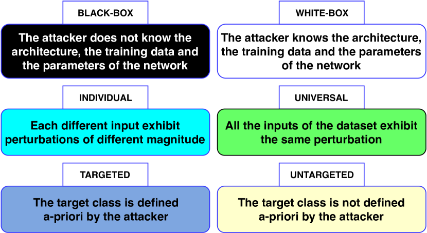
Szegedy et al. (2014) studied that several machine learning models are vulnerable to adversarial examples. Goodfellow et al. (2015) explained the problem observing that machine learning models misclassify examples that are only slightly different from correctly classified examples drawn from the data distribution. Considering an input example $x$, the adversarial example $x^{*}=x+\eta$ is equal to the original one, except for a small perturbation $\eta$. The goal of the perturbation is to maximize the prediction error, in order to make the predicted class $C(x)$ different from the target one $C(x^{*})$. In recent years, many methodologies to generate adversarial examples and their respective defense strategies have been proposed (Feinman et al., 2017; Bhagoji et al., 2017a; Bhagoji et al., 2017b). Adversarial attacks can be categorized according to different attributies, e.g., the choice of the class, the kind of the perturbation and the knowledge of the network under attack (Papernot et al., 2017; Yuan et al., 2017). We summarize these attributies in the Figure 2. A simple representation of the attack scenario that we consider throughout this paper is visible in Figure 3. An adversarial attack is very efficient if it is imperceptible and robust: this is the main concept of the analysis conducted by Luo et al. (2018). Their attack modified the pixels in high variance areas, since the human eyes do not perceive their modifications much. Moreover, an adversarial example is robust if the gap between the probabilities of the predicted and the target class is so large that, after an image transformation (e.g., compression or resizing), the misclassification still holds.

Recent works showed that a CapsuleNet is vulnerable to adversarial attacks. Jaesik Yoon (2017) analyzed the CapsuleNet’s accuracy applying Fast Gradient Sign Method (FGSM), Basic Iteration Method (BIM), Least-likely Class Method and Iterative Least-likely Class Method (Kukarin et al., 2017) to the MNIST dataset (LeCunn et al., 1998). Frosst et al. (2017) presented an efficient technique to detect the crafted images on MNIST, Fashion-MNIST (Xiao et al., 2017) and SVHN (Netzer et al., 2011) datasets.

2 Analysis: Affine Transforming the Images

Before studying the vulnerability of the CapsuleNet under adversarial examples, we apply some affine transformations to the test input images of the GTSRB dataset and observe their effects on our network predictions. We use three different types of transformations: rotation, shift and zoom. This analysis is important to understand how affine transformations, which are perceptible yet plausible in the real world, can or cannot mislead the networks under investigation.

2.1 Experimental Setup

We consider the architecture of the CapsuleNet, as shown in Figure 1. It is composed of a convolutional layer, with kernel $9\times 9$, a convolutional capsule layer, with kernel $5\times 5$, and a fully connected capsule layer. We implement it in TensorFlow, to perform classification on the GTSRB dataset (Kumar et al., 2018). This dataset has images of size $32\times 32$ and it is divided into 34799 training examples and 12630 testing examples. Each pixel intensity assumes a value from 0 to 1. The number of classes is 43. For evaluation purposes, we compare the CapsuleNet with a 5-layer CNN (LeNet) (Ameen, 2018), trained for 30 epochs, and a 9-layer CNN (VGGNet) (Ameen, 2018), trained for 120 epochs. They are both implemented in TensorFlow and their accuracy with clean test images are 91.3% and 97.7%, respectively.

2.2 Robustness under Affine Transformations

(a)

(b)

Figure 4: Affine transformations on the test images, with the corresponding classification predictions made by the CapsuleNet, the VGGNet and the LeNet. (a) Example of a “30 km/h speed limit” sign. (b) Example of a “Stop” sign.

Some examples of affine transformations applied to the input are shown in Figure 4. The analysis shows that both the CapsuleNet and the VGGNet can be fooled by some affine transformations, like zoom or shift. while the confidence of the CapsuleNet is lower. Moreover, the LeNet, since it has lower number of layers, compared to the VGGNet, is more vulnerable to this kind of transformations, as we expected. The CapsuleNet, with capsules and advanced algorithms, such has the so-called routing-by-agreement, is able to overcome the lower complexity, in terms of number of layers and parameters, compared to the VGGNet. Indeed, as we can notice in the example of the image rotated by 30^∘ of Figure 4b, the confidence is lower, but both the CapsuleNet and the VGGNet are able to classify correctly, while the LeNet is fooled.

3 Generation of Targeted Imperceptible and Robust Adversarial Examples

An efficient adversarial attack can generate imperceptible and robust examples to fool the network. Before describing the details of our algorithm, we discuss the importance of these two concepts.

3.1 Imperceptibility and Robustness

An adversarial example can be defined imperceptible if the modifications of the original sample are so small that humans cannot notice them. To create an imperceptible adversarial example, we need to add the perturbations in the pixels of the image with the highest standard deviation. In fact the perturbations added in high variance zones are less evident and more difficult to detect with respect to the ones applied in low variance pixels. Considering an area of $M\cdot N$ pixels x, the standard deviation ($SD$, Equation 1) of the pixel $x_{i,j}$ can be computed as the square root of the variance, where $\mu$ is the average of the $M\cdot N$ pixels:

$$SD(x_{i,j})=\sqrt{\frac{\sum\limits_{k=1}^{M}\sum\limits_{l=1}^{N}(x_{k,l}-\mu)^{2}-(x_{i,j}-\mu)^{2}}{M\cdot N}}$$ (1)

Hence, when the pixel is in a high variance region, its standard deviation is high and the probability to detect a modification of the pixel is low. To measure the imperceptibility, it is possible to define the distance ($D$, Equation 2) between the original sample X and the adversarial sample X*, where $\delta_{i,j}$ is the perturbation added to the pixel $x_{i,j}$:

$$D(X^{*},X)=\sum\limits_{i=1}^{M}\sum\limits_{j=1}^{N}\frac{\delta_{i,j}}{SD(x_{i,j})}$$ (2)

This value indicates the total perturbation added to all the pixels under consideration. We define also $D_{MAX}$ as the maximum total perturbation tolerated by the human eye.

An adversarial example can be defined robust if the gap function, i.e., the difference between the probability of the target class and the maximum class probability is maximized:

$$GAP=P(target\,class)-max\{P(other\,classes)\}$$ (3)

If the gap function increases, the adversarial example becomes more robust, because the modifications of the probabilities caused by some image transformations (e.g., compression or resizing) tend to be less effective. Indeed, if the gap function is high, a variation of the probabilities could not be sufficient to achieve a misclassification.

3.2 Generation of the Adversarial Examples

Figure 5: Our algorithm to generate adversarial examples. The blue-colored boxes are aimed to fool the network, while the green-colored boxes control the imperceptibility of the adversarial attack, whose images at the various stages are represented in the red boxes.

Algorithm 1 : Our Algorithm for Generating Adversarial Attacks

  Given: original sample X, maximum human perceptual distance $D_{MAX}$, noise magnitude $\delta$, $M\cdot N$ pixels, target class, P, V

  while $D(X^{*},X)<D_{MAX}$ do

     -Compute Standard Deviation SD for every pixel

     -Select a subset P of pixels included in the area of $M\cdot N$ pixels with the highest SD for every channel

     -Compute $GAP$, $GAP(-)$, $GAP(+)$

     if $GAP(-)>GAP(+)$ then

        $VariationPriority(x_{i,j})=[GAP(-)-GAP]\cdot SD(x_{i,j})$

     else

        $VariationPriority(x_{i,j})=[GAP(+)-GAP]\cdot SD(x_{i,j})$

     end if

     -Sort in descending order VariationPriority for every channel

     -Select V pixels with highest VariationPriority between the three channels

     if $GAP(-)>GAP(+)$ then

        Subtract noise with magnitude $\delta$ from the pixel in the respective channel

     else

        Add noise with magnitude $\delta$ to the pixel in the respective channel

     end if

     -Compute $D(X^{*},X)$ as the sum of the $D(X^{*},X)$ of every channel

     -Update the original example with the adversarial one

  end while

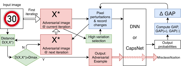
We propose an iterative algorithm that automatically generates targeted imperceptible and robust adversarial examples in a black-box scenario, i.e., we assume that the attacker has access to the input image and to the output probabilities vector, but not to the network model. Our algorithm is shown in Figure 5 and Algorithm 1. The goal of our iterative algorithm is to modify the input image to maximize the gap function (imperceptibility) until the distance between the original and the adversarial example is under $D_{MAX}$ (robustness). The algorithm takes in account the fact that every pixel is composed of three different values, since the images are based on three channels. Compared to the algorithm proposed by Luo et al. (2018), our attack is applied to a set of pixels with the highest standard deviation at every iteration in order to create imperceptible perturbations. Moreover, our algorithm automatically decides if it is more effective to add or subtract the noise, to maximize the gap function, according to the values of two parameters, $GAP(+)$ and $GAP(-)$. These modifications increase the imperceptibility and the robustness of the attack. For the sake of clarity, we also have expressed the formula used to compute the standard deviation in a more comprehensive form.

Our algorithm is composed of the following steps:

• Select a subset $P$ of pixels, included in the area of $M\cdot N$ pixels, with the highest SD for every channel, so that their possible modification is difficult to detect.

• Compute the gap function as the difference between the probability of the target class, chosen as the class with the second highest probability, and the maximum output probability.

• For each pixel of P, compute $GAP(+)$ and $GAP(-)$: these quantities correspond to the values of the gap function, estimated by adding and by subtracting, respectively, a perturbation unit to each pixel. These gaps are useful to decide if it is more effective to add or subtract the noise. For each pixel of P, we consider the greatest value between $GAP(+)$ and $GAP(-)$ to maximize the distance between the two probabilities.

• For each pixel of $P$, calculate the Variation Priority by multiplying the gap difference to the SD of the pixel. This quantity indicates the efficacy of the pixel perturbation.

• For every channel, the $P$ values of Variation Priority are ordered and the highest V values, between the three channels, are perturbed.

• Starting from $3\cdot P$ values of Variation Priority, only V values are perturbed. According to the highest value of the previous computed $GAP(+)$ and $GAP(-)$, the noise is added or subtracted.

• Once the original input image is replaced by the adversarial one, the next iteration starts. The iterations continue until the distance $D$ overcomes $D_{MAX}$.

4 Evaluating our Attack algorithm

4.1 Experimental Setup

We apply our algorithm, showed in Section 3.2, to the previously described CapsuleNet, LeNet and VGGNet. To verify how our algorithm works, we test it on two different examples. We consider M=N=32, because the GTRSB dataset is composed of 32$\cdot$32 images, P=100 and V=20. The value of $\delta$ is equal to the 10% of the maximum value between all the pixels. The parameter $D_{MAX}$ depends on the SD of the pixels of the input image: its value changes according to the different examples because $D(X^{*},X)$ does not increase in the same way for each example.

4.2 Our algorithm applied to the CapsuleNet

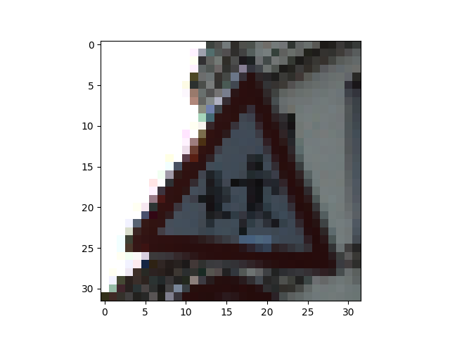
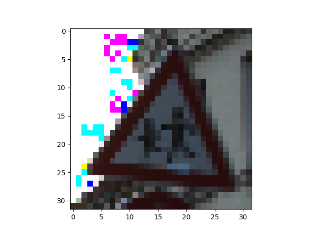
We test the CapsuleNet on two different examples, shown in Figures 6a (Example 1) and 6e (Example 2). For the first one, we distinguish two cases, in order to test whether our algorithm works independently from the target class, and if the final results are different:

• Case I: the target class is the class relative to the second highest probability between all the initial output probabilities.

• Case II: the target class is the class relative to the fifth highest probability between all the initial output probabilities.

(a)

(b)

(c)

(d)

(e)

(f)

(g)

Figure 6: Images for the attack applied to the CapsuleNet: (a) Original input image of Example 1. (b) Image misclassified by the CapsuleNet at the iteration 13 for Case I. (c) Image misclassified by the CapsuleNet at the iteration 16 for Case I. (d) Image at the iteration 12 for Case II. (e) Original input image for Example 2.
(f) Image at the iteration 5, applied to the CapsuleNet. (g) Image misclassified by the CapsuleNet at iteration 21.

(a)

(b)

(c)

Figure 7: CapsuleNet results: (a) Output probabilities of the Example 1 - Case I: blue bars represent the starting probabilities, orange bars the probabilities at the point of misclassification and yellow bars at the $D_{MAX}$.
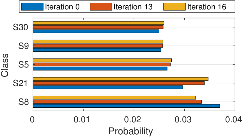
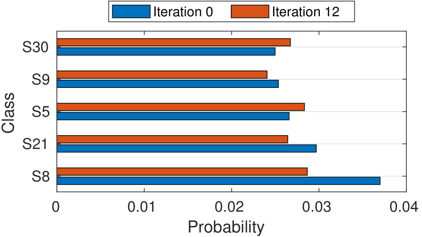
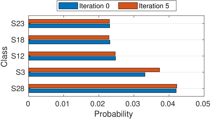
(b) Output probabilities of the Example 1 - Case II: blue bars represent the starting probabilities and orange bars the probabilities at the $D_{MAX}$. (c) Output probabilities of the Example 2: blue bars represent the starting probabilities, and orange bars the probabilities at the $D_{MAX}$.

By analyzing the examples in Case I and Case II, we can observe that:

1. The CapsuleNet classifies the input image shown in Figure 6a as “120 km/h speed limit” (S8) with a probability equal to 0.0370.

   For the Case I, the target class is “Double curve” (S21) with a probability equal to 0.0297. After 13 iterations of our algorithm, the image (in Figure 6b) is classified as “Double curve” with a probability equal to 0.0339. Hence, the probability of the target class has overcome the initial one, as shown in Figure 7a. At this step, the distance $D(X^{*},X)$ is equal to 434.20. Increasing the number of iterations, the robustness of the attack increases as well, because the gap between the two probabilities increases, but also the perceptibility of the noise becomes more evident. After the iteration 16, the distance grows above $D_{MAX}=520$: the sample is represented in Figure 6c.

   For the Case II, the probability relative to the target class “Beware of ice/snow” (S30) is equal to 0.0249, as shown in Figure 7b. The gap between the maximum probability and the probability of the target class is higher than the gap in Case I. After 12 iterations, the network has not misclassified the image yet (see Figure 6d). In Figure 7b we can observe that the gap between the two classes has decreased, but not enough for a misclassification. However, at this iteration, the value of the distance overcomes $D_{MAX}=520$. In this case, we show that our algorithm would need more iterations to misclassify, at the cost of more perceivable perturbations.

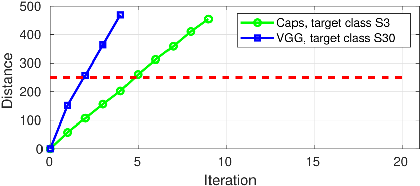
2. The CapsuleNet classifies the input image shown in Figure 6e as “Children crossing” (S28) with a probability equal to 0.042. The target class is “60 km/h speed limit” (S3) with a probability equal to 0.0331. After 5 iterations, the distance overcomes $D_{MAX}=250$, while the network has not misclassified the image yet (see Figure 6f), because the probability of the target class does not overcome the initial maximum probability, as shown in Figure 7c. The misclassification appears at the iteration 21, when the sample (see Figure 6g). However, the perturbation is very percievable.

4.3 Our algorithm applied to a 9-layer VGGNet and a 5-layer LeNet

(a)

(b)

(c)

(d)

(e)

(f)

(g)

Figure 8: Images for the attack applied to the CNNs: (a) Original input image for Example 1 (b) Image at the iteration 3, applied to the VGGNet. (c) Image at the iteration 9, misclassified by the VGGNet. (d) Original input image for Example 2. (e) Image at the iteration 2, applied to the VGGNet. (a) Image at the iteration 6, misclassified by the LeNet.. (b) Image at the iteration 13, misclassified by the LeNet.

(a)

(b)

(c)

Figure 9: CNNs results. (a) Output probabilities of the Example 1 on the VGGNet: blue bars represent the starting probabilities, orange bars the probabilities at the point of misclassification and yellow bars at the $D_{MAX}$. (b) Output probabilities of the Example 2 on the VGGNet: blue bars represent the starting probabilities and orange bars the probabilities at the $D_{MAX}$. (c) Output probabilities of the Example 1 on the LeNet: blue bars represent the starting probabilities, orange bars the probabilities at the point of misclassification and yellow bars at the $D_{MAX}$.

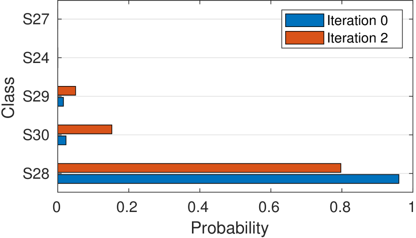
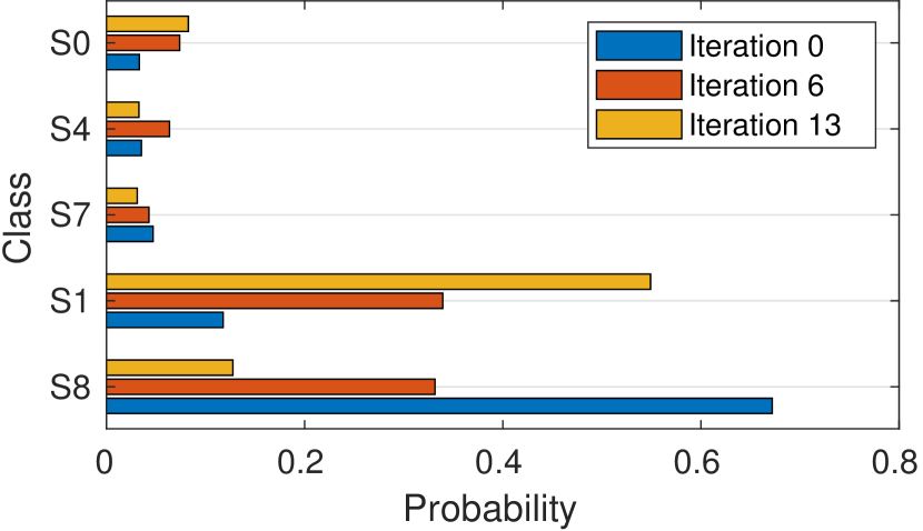
To compare the robustness of the CapsuleNet and the 9-layer VGGNet, we choose to evaluate the previous two examples, which have been applied to the CapsuleNet. For the Example 1, we consider only the Case I as benchmark. The VGGNet classifies the input images with different output probabilities, compared to the ones obtained by the CapsuleNet. Therefore, our metric to evaluate how much the VGGNet is resistant to our attack is based on the value of the gap at the same distance.

To compare the robustness of the CapsuleNet and the 5-layer LeNet, we only consider the Example 1, because the Example 2 is already classified incorrectly by the LeNet. Applying our algorithm to the LeNet, we observe that, as expected, it is more vulnerable than the CapsuleNet and the VGGNet.

We can make the following considerations on our examples:

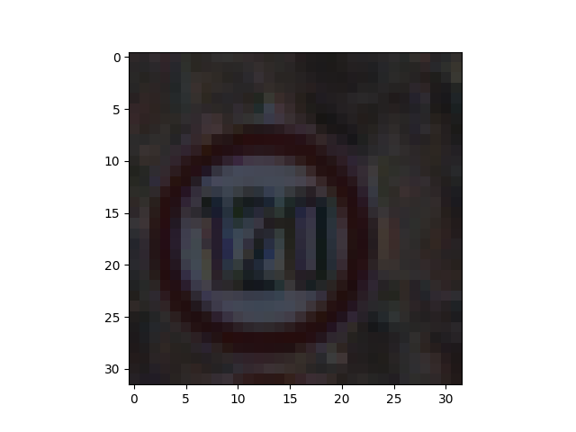
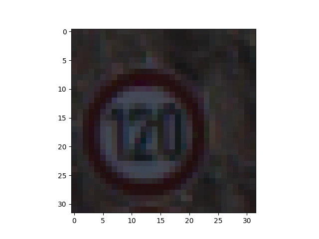
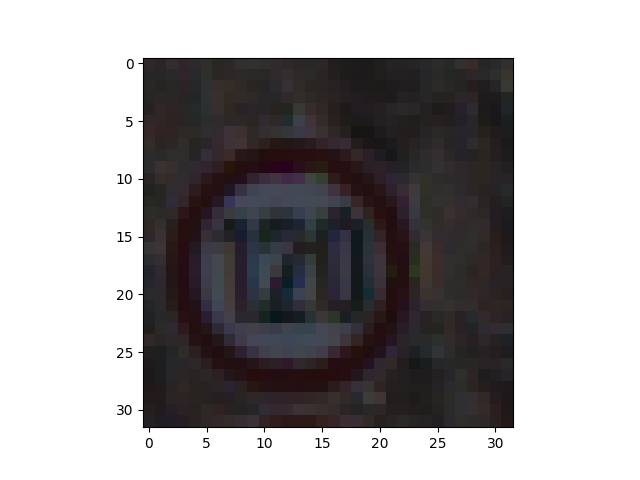
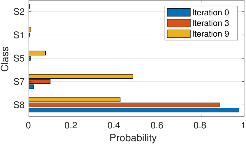
1. The VGGNet classifies the input image (in Figure 8a) as “120 km/h speed limit” (S8) with a probability equal to 0.976. The target class is “100 km/h speed limit” (S7) with a probability equal to 0.021. After 3 iterations, the distance overcomes $D_{MAX}=520$, while the VGGNet has not misclassified the image yet (see Figure 8b) yet: our algorithm would need to perform more iterations before fooling the VGGNet, since the two initial probabilities were very distant, as shown in Figure 9a. Such scenario appears after 9 iterations (in Figure 8c), where the probability of the target class is 0.483.

2. The VGGNet classifies the input image (in Figure 8d) as “Children crossing” (S28) with a probability equal to 0.96. The target class is “Beware of ice/snow” (S30) with a probability equal to 0.023. After 2 iterations, the distance overcomes $D_{MAX}=250$, while the VGGNet has not misclassified the image yet (see Figure 8e). As in the previous case, this scenario is due to the high distance between the initial probabilities, as shown in Figure 9b. We can also notice that the VGGNet reaches $D_{MAX}$ in a lower number of iterations, as compared to the CapsuleNet.

3. The LeNet classifies the input image (in Figure 8a) as “120 km/h speed limit” (S8) with a probability equal to 0.672. The target class is “30 km/h speed limit” (S1) with a probability equal to 0.178. After 6 iterations, the perturbations fool the LeNet, because the image (In Figure 8f), is classified as the target class with a probability equal to 0.339. The perturbations become perceptible after 13 iterations (Figure 8g), where the distance overcomes $D_{MAX}=520$.

(a)

(b)

Figure 10: (a) $D(X^{*},X)$ behavior for the Example 1. (b) $D(X^{*},X)$ behavior for the Example 2.

4.4 Comparison and results

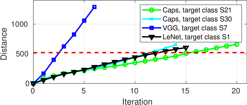
From our analyses, we can observe that the vulnerability of the 9-layer VGGNet to our adversarial attack is slightly lower than the vulnerability of the CapsuleNet, since the former one requires more perceivable perturbations to be fooled. Our observation is remarked by the graphs in Figure 10: the value of $D(X^{*},X)$ increases more sharply for the VGGNet than for the CapsuleNet. Hence, the perceivability of the noise in the image can be measured as the value of $D(X^{*},X)$ divided by the number of iterations: the noise in the VGGNet becomes perceivable after few iterations. Moreover, we can observe that the choice of the target class plays a key role for the success of the attack.

We notice that other features that evidence the differences between the VGGNet and the CapsuleNet are crucial. The VGGNet is deeper and contains a larger number of weights, while the CapsuleNet can achieve a similar accuracy with a smaller footprint. This effect causes a disparity in the prediction confidence between the two networks. It is clear that the CapsuleNet has a much higher learning capability, compared to the VGGNet, but this phenomena does not reflect to the prediction confidence. Indeed, comparing Figures 7 and 9, we can notice that the output probabilities predicted by the CapsuleNet are close to each other, even more than the LeNet. However, the perturbations does not affect the output probabilities of the CapsuleNet as much as for the cases of the CNNs. The LeNet, as expected, even though it has a similar depth and similar number of parameters, is more vulnerable than the CapsuleNet.

Moreover, recalling from Section 2, we observed that the VGGNet and the CapsuleNet are more resistant than the LeNet to the affine transformations: this behavior is consistent with the results obtained applying our adversarial attack algorithm.

5 Conclusions

In this paper, we proposed an algorithm to generate targeted adversarial attacks in a black box scenario. We applied our attack to the GTSRB dataset and we verified its impact on a CapsuleNet, a 5-layer LeNet and a 9-layer VGGNet. Our experiments show that the CapsuleNet appears more robust than the LeNet to the attack, but slightly less than the VGGNet, because the modifications of the pixels in the traffic signs are less perceivable when our algorithm is applied to the CapsuleNet, rather than to the VGGNet. A serious issue for the CapsuleNet is that the gap between the output probabilities is lower than the one computed on the VGGNet predictions. However, the change in absolute values of the probabilities at the output of the CapsuleNet is lower than their changes in the VGGNet. Hence, further modifications of the CapsuleNet algorithm, aiming to increase the prediction confidence, would be beneficial to improve its robustness.

References

- [1] G. E. Hinton, A. Krizhevsky, and S. D. Wang. Transforming auto-encoders. In ICANN, 2011.
- [2] G. E. Hinton, N. Frosst, and S. Sabour. Matrix capsules with em routing. In ICLR, 2018.
- [3] S. Houben, J. Stallkamp, J. Salmen, M. Schlipsing, and C. Igel. Detection of traffic signs in real-world images: The German Traffic Sign Detection Benchmark. In IJCNN, 2013.
- [4] A. D. Kumar, R. Karthika, and L. Parameswaran. Novel deep learning model for traffic sign detection using capsule networks. arXiv preprint arXiv:1805.04424, 2018.
- [5] S. Sabour, N. Frosst, and G. E. Hinton. Dynamic routing between capsules. In NIPS, 2017.
- [6] A. Shafahi, W. R. Huang, C. Studer, S. Feizi, and T. Goldstein. Are adversarial examples inevitable? arXiv preprint arXiv:1809.02104, 2018.
- [7] I. Goodfellow, J. Shlens and C. Szegedy. Explaining and harnessing adversarial examples. In ICLR, 2015.
- [8] A. Kukarin, I. Goodfellow and S. Bengio. Adversarial examples in the physical world. In ICLR, 2017.
- [9] N. Frosst, S. Sabour, G. Hinton. DARCCC: Detecting Adversaries by Reconstruction from Class Conditional Capsules, arXiv preprint arXiv:1811.06969, 2018.
- [10] N. Papernot, P. McDaniel, I. Goodfellow, S. Jha, Z. Celik, and A. Swami. Practical Black-Box Attacks against Machine Learning. In ACM Asia Conference on Computer and Communications Security, 2017.
- [11] Bo Luo, Yannan Liu, Lingxiao Wei, and Qiang Xu. Towards Imperceptible and Robust Adversarial Example Attacks against Neural Networks. arXiv preprint arXiv:1801.04693, 2018.
- [12] R. Feinman, R. Curtin, S. Shintre, and A. Gardner. Detecting adversarial examples from artifacts. arXiv preprint arXiv:1703.00410, 2017.
- [13] A. Bhagoji, D. Cullina, and P. Mittal. Dimensionality reduction as a Defense against Evasion Attacks on Machine Learning Classifiers. arXiv preprint arXiv:1704.02654, 2017a.
- [14] A. Bhagoji, D. Cullina, C. Sitawarin and P. Mittal. Enhancing Robustness of Machine Learning Systems via Data Transformations. arXiv preprint arXiv:1704.02654, 2017b.
- [15] C. Szegedy, W. Zaremba, and I. Sutskever. Intriguing properties of neural networks. In ICLR, 2014.
- [16] X. Yuan, P. He, Q. Zhu, R. R. Bhat, and X. Li. Adversarial examples: Attacks and defenses for deep learning. arXiv preprint arXiv:1712.07107, 2017.
- [17] R. Mukhometzianov, and J. Carrillo. CapsNet comparative performance evaluation for image classification. arXiv preprint arXiv 1805.11195, 2018.
- [18] Jaesik Yoon. Adversarial Attack to Capsule Networks project. Available online at: https://github.com/jaesik817/adv_attack_capsnet, 2017.
- [19] A. Bhandare, M. Bhide, P. Gokhale, and R. Chandavarka. Applications of Convolutional Neural Networks, In IJCSIT, 2016.
- [20] N. Carlini, P. Mishra, T. Vaidya, Y. Zhang, M.Sherr, C. Shields, D. Wagner, and W. Zhou. Hidden voice commands. In USENIX Security Symposium, 2016.
- [21] G. Zhang, C. Yan, X. Ji, T. Zhang, T. Zhang, and W. Xu. DolphinAttack: Inaudible voice commands. arXiv preprint arXiv:1708.09537, 2017.
- [22] H. Xiao, K. Rasul, and R. Vollgraf. Fashion-mnist: a novel image dataset for benchmarking machine learning algorithms. In CoRR abs/1708.07747, 2017.
- [23] Y. LeCun, L. Bottou, Y. Bengio, and P. Haffner. Gradient-based learning applied to document recognition. In Proceedings of the IEEE, 1998.
- [24] Y. Netzer, T. Wang, A. Coates, A. Bissacco, B. Wu, and A. Y. Ng. Reading digits in natural images with unsupervised feature learning. In NIPS Workshop on Deep Learning and Unsupervised Feature Learning, 2011.
-
[25]
M. Ameen, German-traffic-sign-classification-using-Tensorflow,
https://github.com/mohamedameen93/German-Traffic-Sign-Classification-Using-TensorFlow, 2018.