Parallelization and scalability analysis of inverse factorization using the Chunks and Tasks programming model††thanks: \fundingThis work was supported by the Swedish research council under grant 621-2012-3861 and the Swedish national strategic e-science research program (eSSENCE).
Abstract
We present three methods for distributed memory parallel inverse factorization of block-sparse Hermitian positive definite matrices. The three methods are a recursive variant of the AINV inverse Cholesky algorithm, iterative refinement, and localized inverse factorization, respectively. All three methods are implemented using the Chunks and Tasks programming model, building on the distributed sparse quad-tree matrix representation and parallel matrix-matrix multiplication in the publicly available Chunks and Tasks Matrix Library (CHTML). Although the algorithms are generally applicable, this work was mainly motivated by the need for efficient and scalable inverse factorization of the basis set overlap matrix in large scale electronic structure calculations. We perform various computational tests on overlap matrices for quasi-linear Glutamic Acid-Alanine molecules and three-dimensional water clusters discretized using the standard Gaussian basis set STO-3G with up to more than 10 million basis functions. We show that for such matrices the computational cost increases only linearly with system size for all the three methods. We show both theoretically and in numerical experiments that the methods based on iterative refinement and localized inverse factorization outperform previous parallel implementations in weak scaling tests where the system size is increased in direct proportion to the number of processes. We show also that compared to the method based on pure iterative refinement the localized inverse factorization requires much less communication.
1 Introduction
We focus in this work on the efficient and scalable computation of inverse factors of symmetric positive definite matrices. Although the methods considered are generally applicable, we are in particular interested in the factorization of basis set overlap matrices coming from discretizations using localized basis sets in large scale electronic structure calculations based on, for instance, Hartree–Fock [19] or Kohn–Sham density functional theory [17]. In this context, the inverse factor is used in a congruence transformation of the Roothaan–Hall/Kohn–Sham eigenvalue equations:
| (1) |
where is the Fock or Kohn–Sham matrix, is the overlap matrix, and is an inverse factorization thereof.
Electronic structure theory is of fundamental importance in a number of scientific disciplines, including biology, chemistry, and materials science. Unfortunately, the solution of the quantum mechanical eigenvalue problem outlined above using standard methods is extremely expensive and usually limited to rather small molecular systems. To be able to reach larger molecular systems and materials there are essentially two possibilities: reduce the computational workload or increase the computational power. The workload of standard electronic structure methods increases cubically with system size. This means that an increase of the computational power alone has a very limited effect on the system sizes that are within reach. Therefore, so-called linear scaling methods have been developed for which the workload increases only linearly with system size. A remarkable progress of such methods has occurred in the last 15-20 years, see [8] for an excellent overview of this development. With a linear scaling method at hand it makes sense to attempt to reach larger systems by increasing the computational power. Today this is possible only with a parallel implementation. Ideally, the runtime should stay constant as the workload is increased in direct proportion to the number of processors; this is sometimes referred to as linear weak scaling efficiency. With both linear scaling of the total workload with system size and linear weak scaling efficiency, the system sizes within reach should increase linearly with the computational power employed. Therefore, our primary criteria for assessment of the developed methods are scaling with system size and weak scaling efficiency. With the current trend that the cost of floating point operations relative to the cost of movement of data is becoming smaller we shall also consider the communication costs to be important.
Two approaches have dominated previous work on inverse factorization of the overlap matrix. The first one is computation of the inverse Cholesky factor using the AINV algorithm [6]. The inverse Cholesky factor has frequently been used in electronic structure calculations [20, 10, 30]. There are several variants of the AINV algorithm including a stabilized one [4], a blocked one [5] and a recursive one [26], where the latter is suitable for hierarchical matrix representations. The AINV algorithms are very fast but, as will be shown in the present work, the parallelism in those algorithms is limited. The second approach is computation of the inverse square root using an iterative refinement method [21] closely related to the Newton–Schulz iteration for the sign matrix function [15, 22]. This method is based on sparse matrix-matrix multiplication and has also been frequently used in electronic structure calculations, using a scaled identity matrix as starting guess [16, 29].
A third alternative is recursive inverse factorization which is a divide-and-conquer method that combines iterative refinement with a recursive decomposition of the matrix [23]. The matrix is partitioned using a binary principal submatrix decomposition, corresponding to a cut of the index set into two pieces. Inverse factors of the two principal submatrices are computed and iterative refinement is then used in a correction step to get an inverse factor of the whole matrix. This procedure is applied recursively giving the recursive inverse factorization algorithm. Recently a localized variant of this method was proposed which uses only localized computations for the correction step with cost proportional to the cut size [22]. We refer to this variant as localized inverse factorization. A key feature of both the regular and localized recursive inverse factorization is that the inverse factorizations at lower levels are completely disconnected and therefore embarrassingly parallel.
We consider in this work one variant in each of the three classes of methods outlined above: 1) the recursive variant of the AINV algorithm, hereinafter referred to as the recursive inverse Cholesky algorithm (RINCH), 2) iterative refinement using a scaled identity as starting guess (IRSI), and 3) localized inverse factorization (LIF). All three alternatives considered here make use of sparse matrix-matrix multiplication as a computational kernel.
Sparse matrix-matrix multiplication for general matrices with a priori unknown sparsity patterns is difficult to parallelize, especially with good weak scaling performance and taking advantage of data locality [3]. A common approach is to randomly permute rows and columns of the input matrices to destroy any structure. Then, some algorithm for dense matrices, such as Cannon’s algorithm or SUMMA, is applied, but with the dense submatrix products replaced by sparse submatrix products [9, 7]. In this way load balance is achieved. Linear weak scaling efficiency is possible if, instead of the two-dimensional process grid used in Cannon’s algorithm and SUMMA, a three-dimensional process grid is used as in [3, 2, 11]. However, because of the random permutation of matrix rows and columns, the possibility to exploit the nonzero structure to avoid movement of data or communication is lost.
In this article we build on our previous work on a sparse matrix library based on sparse quaternary tree (quad-tree) matrix representation implemented using the Chunks and Tasks programming model [24, 25]. The library is called the Chunks and Tasks Matrix Library (CHTML) and is publicly available at chunks-and-tasks.org under the modified BSD license. This implementation exploits data locality to achieve efficient representation of sparse matrices. For sparse matrix-matrix multiplication, this leads to much less movement of data compared to approaches that do not take advantage of data locality. In particular, for matrices with data locality, such as overlap matrices or other matrices coming from discretizations of physical systems using localized basis sets, the average amount of data received per process is constant in the weak scaling scenario outlined above where the number of processors is scaled up in direct proportion to the system size. The total execution time is instead usually dominated by the execution of tasks along the critical path. For the iterative refinement this scaling behavior should be directly inherited. For the localized inverse factorization the localization in the computation is even stronger with the bulk of the work lying in subproblems that are completely disconnected. In theory very little communication should therefore be needed in a parallel implementation of the localized inverse factorization algorithm. In practice, using a traditional message passing approach, it would be very difficult to achieve a parallel implementation of the localized inverse factorization algorithm with a balanced distribution of both work and data for sparse matrices with a priori unknown sparsity patterns. We show in this article, using instead a Chunks and Tasks implementation, that reduced communication costs compared to other scalable algorithms can be realized in practice.
We have implemented the recursive inverse Cholesky algorithm, the iterative refinement method, and localized inverse factorization in CHTML. In Section 2 we describe the three algorithms. In Section 3 we analyse the scalability of the algorithms by considering their critical paths. We are in particular interested in how the critical paths depend on system size, since this puts a limit on the weak scaling performance that can be achieved. In Section 4 we give some background to the choice of programming model and dicuss some restrictions in the model and their implications for expressiveness and performance. In Section 5 we present numerical experiments for overlap matrices coming from discretizations using standard Gaussian basis sets, for quasi-linear Glutamic Acid-Alanine molecules as well as three-dimensional water clusters. It is shown that all three methods achieve linear scaling with system size for the considered systems. Weak scaling and actual critical path lengths as reported by the Chunks and Tasks library are compared to the theoretical results. We end the article with a discussion and some concluding remarks in Section 6.
2 Algorithms
In this section we describe the inverse factorization algorithms considered in this work. All algorithms are written such as to operate on matrices represented using quad-trees.
2.1 The recursive inverse Cholesky algorithm
The recursive inverse Cholesky algorithm (RINCH) [26] is a variant of the AINV algorithm that is adapted to hierarchical matrix structures and uses recursive calls to go through the hierarchy. We use here the left-looking variant of RINCH given by Algorithm 1. This algorithm is equivalent to Algorithm 7 in [26] with blocks in every dimension. When reaching the leaf level of the hierarchy, instead of the recursive call, one may for instance use the regular non-recursive AINV or routines for Cholesky factorization and inversion of triangular matrices in the Basic Linear Algebra Subprograms (BLAS) to compute the inverse factor of the leaf matrix. The most common operation in the algorithm is matrix-matrix multiplication, which, besides the recursive RINCH calls, is also the most time-consuming operation.
2.2 Iterative refinement
The refinement procedure proposed in [21] can be used to improve the accuracy of an approximate inverse factor. The procedure works as follows: given as an approximation of the inverse factor of such that a sequence of matrices is constructed such that the factorization error as The regular iterative refinement is given by
| (2) |
If it is known that only a small part of the matrix needs to be updated, then one can use a localized method in order to reduce costs:
| (3) |
One possible choice for the starting guess is a scaled identity matrix
| (4) |
which with an appropriate scaling gives the inverse square root of the matrix as a result [14, 16]. The optimal scaling is given by
| (5) |
where and are the extremal eigenvalues of [23].
In our case the exact eigenvalues are not available and we will use an approximation for the scaling factor suggested in [16]:
| (6) |
where is an approximation of the spectral radius of computed with the Gershgorin circle theorem [13].
In order to minimize the number of parameters, we employ the automatic stopping criterion proposed in [18] and used in [22]. The iterative refinement is stopped as soon as . Using this stopping criterion, the iterative refinement process automatically terminates when rounding or other numerical errors start to dominate over the factorization error.
2.3 Recursive and localized inverse factorization
Recursive inverse factorization first described in [23] is based on the following result. Let the input matrix be partitioned as and let , where and are inverse factors of and , respectively. Then, , which implies convergence of iterative refinement with as starting guess [23]. This result was recently strengthened and it was shown that [22]. Those convergence results immediately suggest a recursive inverse factorization algorithm where iterative refinement is combined with a recursive binary principal submatrix decomposition of the matrix .
Recently we proposed a localized variant of the recursive inverse factorization algorithm that makes use of the localized iterative refinement in (3) and a local construction of the starting guess [22]. An advantage of this localized inverse factorization, given by Algorithm 2, is that under certain assumptions on and the recursive principal submatrix decomposition, the cost of combining and to get an inverse factor of becomes negligible compared to the overall cost for sufficiently large systems [22]. Another important feature of this algorithm is that and can be computed in parallel without any communication between the two computations.
When the lowest level is reached in the algorithm, leaf-level routines are called to compute the inverse factor. The leaf level inverse factorization may for example use BLAS routines or some standard AINV algorithm. Alternatively, one may switch to for example the RINCH algorithm before reaching the leaf level of the quad-tree.
3 Estimation of critical path lengths
For any given system, the computational time will be bounded from below by a value determined by the critical path length. Even if one assumes that the runtime is able to exploit all parallelism in the algorithm and that an infinite number of processes are available, the computational time cannot fall below this value. In this section we will derive critical path lengths as a function of system size for each of the three algorithms considered in this work. In this way we get the best possible weak scaling performance for each of the three algorithms.
First of all, let us define a task as a large enough computation, which may consist of child tasks or arithmetical operations, or both. For example, matrix addition is a task and, taking into account matrix representation as a quad-tree, it actually consists of 4 child tasks, which are also matrix additions. Each of those also consists of 4 tasks unless the leaf level of the hierarchy is reached where arithmetical routines are performed. We assume that a task can have multiple inputs and a single output.
Using the definition of a task, the whole computation can be viewed as the traversal of a directed graph, where each vertex is a task and the edges represent data dependencies between tasks. Then, the critical path can be defined as the longest path in the directed graph of the computation, which connects start and end vertices. The critical path is the longest series of operations which has to be executed serially due to data dependencies and its length is an important feature of any algorithm from a parallel programmer’s point of view.
In our derivations, we consider matrix-matrix multiplication, matrix-scalar multiplication, matrix addition, separate matrix transpose and factorization routines as tasks. Small computations like multiplication or addition of real numbers are not considered as tasks. If a matrix transpose is involved in a multiplication, we assume that it does not require a separate task.
Let us derive the critical path estimation for the algorithms described in Section 2. We will start from small examples, then derive recursive formulas and finally obtain estimations for the algorithms. Note that these derivations do not take into account the sparsity of the matrices but are done for dense ones. In practice, the matrices are sparse, and therefore the critical path may be shorter.
3.1 Critical path length for recursive inverse Cholesky
Here we consider the critical path length of the RINCH algorithm. In Algorithm 1, on every level of recursion, there are 3 matrix-matrix multiplication operations (lines 6,7 and 9) that cannot be performed in parallel and 3 matrix-scalar multiplication or matrix addition operations (lines 7 and 9). Finally, one has to do 2 recursive calls that also cannot be done in parallel because of data dependencies. The critical path will for large systems be dominated by the matrix-matrix multiplications and the recursive calls.
Let us denote the total critical path length by , where is the matrix size. We assume that the critical path length of a matrix-matrix multiplication task depends on the matrix size and we will denote it as . On the lowest level of recursion, where the leaf matrices are reached, instead of calling the task itself, one calls leaf-level routines. We will treat these routines as tasks with critical path length 1.
For simplicity we also assume that the leaf level matrices are of size and that the number of non-leaf levels in the hierarchy is equal to . Also, this leads to and , or, in other words, all leaf-level routines have a critical path of length 1. Operations like matrix addition or matrix-scalar multiplication, where each node in the matrix quad-tree is visited only once, have critical path length . For simplicity we will assume that the matrix dimension is equal to a power of .
For example, if we have a matrix, then the total length of the critical path can be written as
| (7) |
If one increases the matrix size by a factor 2, then
| (8) |
Let us denote by the critical path length of all non-RINCH tasks on the current level of hierarchy. In our case,
i.e. we have 3 matrix-matrix multiplications of matrices and 3 operations with critical path length . By we will denote the number of recursive RINCH calls on the current level. Note that none of them can be done in parallel and therefore the critical path length can then be written as
| (9) |
which gives
| (10) |
The critical path length of matrix-matrix multiplication with a quad-tree matrix representation scales as a second order polynomial in [25] and therefore for some constants independent of . Combining this with (10) gives the critical path length for the RINCH algorithm:
| (11) |
For full derivation see Appendix A. Clearly, the critical path length grows linearly with system size, i.e. in the sense of algorithm complexity analysis.
3.2 Critical path length for iterative refinement
Here we consider the critical path length of the IRSI algorithm. We have already mentioned that the critical path length of matrix-matrix multiplication with a quad-tree matrix representation scales as a second order polynomial in [25]. Since the iterative refinement procedure has matrix-matrix multiplication as dominating operation, and assuming that the number of iterations does not depend on , its critical path length scales the same way.
3.3 Critical path length for localized inverse factorization
Here we derive the critical path length of the LIF algorithm. Let us first consider a single iterative refinement iteration (lines 10 to 13 of Algorithm 2). Each construction of the correction matrix and update of the inverse factor (lines 10 and 11) requires matrix-matrix multiplications, matrix-scalar multiplications and matrix additions. Thus, this update has a critical path of length , where is the critical path length of the matrix-matrix multiplication and is the matrix size at the current level of the hierarchy. The update of the -matrix (line 12) has critical path length since only two matrix-matrix multiplications cannot be done in parallel. Since cannot be updated until has been updated, the total critical path length of a single iteration is
| (12) |
It was shown in [22] that the number of iterative refinement iterations needed to reach an accuracy is bounded by
| (13) |
at any level in the hierarchy. If the condition number of is bounded by a constant independent of then is also bounded by a constant independent of . For simplicity of exposition we will in the following assume that the number of iterative refinement iterations is exactly equal to at all levels and branches of the recursion. Then, the critical path length of the localized iterative refinement procedure is given by
| (14) |
Apart from refinement of the inverse factor, one has to prepare initial guesses for the refinement. The construction of (line 7 of Algorithm 2) requires 2 matrix-matrix multiplications of matrices of size , a separate transpose of size and a single multiplication by a scalar. Therefore its critical path length is Then, in order to be able to prepare initial guesses, one also needs to do 2 recursive calls, each with critical path length of
Similarly to the previous algorithm, let us denote by the critical path length of all non-LIF tasks on the current level of the hierarchy:
| (15) |
Then we arrive at the following recursive relation:
| (16) |
where, similarly to the case of RINCH, is the number of recursive calls which cannot be handled in parallel. This form is very similar to (9) and gives us the following non-recursive relation when expanding for arbitrary :
| (17) |
Taking into account the fact that recursive LIF calls do not depend on each other and thus can be performed in parallel, one can set and the expression becomes
| (18) |
Using again the fact that the critical path length of matrix-matrix multiplication with a quad-tree matrix representation scales as a second order polynomial in we have that for some constants independent of . Combining this with (18) gives the critical path length for the localized inverse factorization algorithm:
| (19) |
For full derivations see Appendix B. One can observe that the leading term is and in the sense of algorithm complexity analysis. The critical path length grows slower than linearly.
4 Chunks and Tasks implementation
We implemented the RINCH, IRSI and LIF algorithms using the Chunks and Tasks programming model [24]. Chunks and Tasks is a task-based model suitable for dynamic and hierarchical algorithms that allows a programmer to write parallel code without thinking about synchronization or message passing between different processes. When using this model, the programmer writes the code by defining objects of two classes. Objects of the first class represent pieces of data, while objects of the second class represent pieces of work which is to be done. They are referred to as chunks and tasks, respectively. Each task has one or more input chunks and a single output chunk. Once a chunk has been registered to a runtime library, it is read-only. Identifiers of chunks and tasks are provided by the library and the user cannot modify them. This makes the model free from deadlocks and race conditions. In the present work we use the Chunks and Tasks model as implemented in the proof-of-concept runtime library CHT-MPI, freely available for downloading at http://chunks-and-tasks.org/. The library is written in C++ and parallelized using MPI and Pthreads [24]. A work stealing approach is used to achieve load balancing.
The present work makes use of and extends CHTML [25] implemented using the Chunks and Tasks model. CHTML includes a locality-aware sparse matrix-matrix multiplication implementation that takes advantage of data locality to reduce communication costs. In CHTML, a matrix is represented as a quad-tree and all non-leaf nodes are chunks containing identifiers of child nodes. If a submatrix is zero, then the corresponding identifier is set to the null chunk identifier. Only on the leaf level, chunks contain matrix elements. This approach allows to exploit sparsity patterns dynamically by skipping operations on zero submatrices. We use a block-sparse leaf matrix library for the representation of submatrices at leaf level, as in [25]. This means that each leaf matrix is divided into small blocks and only non-zero blocks are stored in memory.
The Chunks and Tasks programming model enforces certain restrictions on how a program can be implemented. Those restrictions exist both to help the programmer in the development of his program and to make the implementation of efficient runtime libraries feasible. The Chunks and Tasks model is purely functional and does not support global variables. The only way a task can access data, besides compile time constants, is through the input chunks.
Another restriction regards the uninterrupted execution of tasks. A task cannot synchronize with child tasks during its execution. This means that the runtime library can rely on uninterrupted execution of tasks which is important for efficient allocation of resources. For the application programmer this means that while-loop constructs where the termination condition depends on results of child tasks registered in the while loop body cannot be implemented in the usual way. When the number of iterations is limited an alternative is to register a predetermined number of tasks in a for-loop including tasks that check the termination condition. When the termination condition has been reached, the superfluous remaining tasks immediately return from their task executions. Otherwise one may encapsulate the body of the while-loop into a task and use recursive registration of tasks. The updated variables are encapsulated in chunks and the chunk identifiers are provided as input to a task of the same type together with all necessary parameters for the recursive task registration. The next modification of the variables happens when a new task is executed. We used this approach for the iterative refinement procedure as applied in the localized inverse factorization, see Algorithm 4. Note that this restriction applies only to task execution. In the main program the execution of a task is a blocking call that waits until all descendant tasks have been executed. Thus, an algorithm like IRSI can be implemented in the standard way.
To illustrate how the Chunks and Tasks code looks and help the reader to understand the essence of the task-based parallel programming, we include pseudocodes, which are simplified versions of the real code but include some of its key characteristics. Algorithm 3 represents RINCH, Algorithm 4 represents IRSI and Algorithm 5 represents LIF correspondingly. The value realmax() in Algorithm 5 represents the largest real value available, it is assigned to the error as the starting value and the error is then gradually reduced. The simplification concerns evaluations of mathematical expressions. In practice, every operation with a matrix is a task which typically generates a whole hierarchy of tasks. We write ”evaluate(expr)” to indicate the registration of tasks needed to evaluate an expression expr. Note that the variables are actually the identifiers of the corresponding chunks. As one can see, the codes consist almost purely of registrations of tasks and, in the end of the day, all tasks will be turned into chunks. The pseudocodes also ignore the necessity to derive tasks from a base task class and implement certain obligatory member functions.
To gain more from modern C++ and make the code flexible when it comes to the choice of the algorithm version, we employed template specialization techniques for specifying the choice instead of making several similar codes. For example, the recursive inverse factorization algorithm can work with either local or non-local refinement.
5 Experimental results
To numerically investigate the scaling behaviour of the algorithms, we used basis set overlap matrices coming from discretizations using Gaussian basis sets for two kinds of molecules, quasi-linear Glutamic Acid-Alanine (Glu-Ala) helices and three-dimensional water clusters. The xyz coordinates, which were partially used in [27], can be downloaded from http://ergoscf.org. The overlap matrices were generated using the Ergo open-source program for linear-scaling electronic structure calculations [28], publicly available at http://ergoscf.org under the GNU Public License (GPL) v3. The computations were done using the standard Gaussian basis set STO-3G, with block-sparse leaf level matrix representation. The calculations were performed in double precision, with leaf matrix size and blocksize . The chunk cache size was set to 4 gigabytes. Moreover, in order to enforce sparsity, truncation of small elements was performed after every matrix-matrix multiplication with threshold and after all calls to leaf level routines. The truncation procedure performs truncation of leaf internal blocks so that the blocks with Frobenius norm smaller than the threshold value are removed. The basis overlap matrix was also truncated with the same threshold, and then factorized. We have already mentioned that in the localized inverse factorization, one may, instead of going down to the leaf level, employ RINCH somewhere higher up in the hierarchy. We did so when the current matrix size became smaller than or equal to 16384. For the iterative refinement we used . The local version of the refinement (3) was used in all calculations. When performing iterative refinement with scaled identity as starting guess (IRSI), we did not take the time needed to compute the Gershgorin bounds into account.
All the computations were performed on the Beskow cluster located at the PDC high performance computing center at the KTH Royal Institute of Technology in Stockholm. The test calculations were performed using a development version of CHT-MPI compiled with the GCC 7.3.0 g++ compiler, Cray MPICH 7.7.0 and OpenBLAS 0.2.20 [1] for leaf-level routines. The OpenBLAS was configured to use a single thread. The Beskow cluster consists of 2060 nodes, where each node has 2 Intel Xeon E5-2698v3 CPUs with 16 cores each running at 2.3 GHz frequency (3.6 GHz with Turbo-boost), with 64 GB of RAM. The nodes are connected with Cray Aries high speed network of Dragonfly topology. In the CHT-MPI library every process uses a set of threads of which some execute tasks and some do auxiliary work like work stealing. We used a single process per node, 31 worker threads per process thus leaving a single core for communication and other auxiliary work.
In some of the figures presented in the following subsections, some data points are missing for one or several methods. This indicates that the calculation was terminated due to insufficient memory. We noted that this happened more often for the RINCH and IRSI methods.
5.1 Scaling with system size
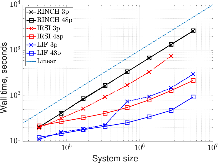
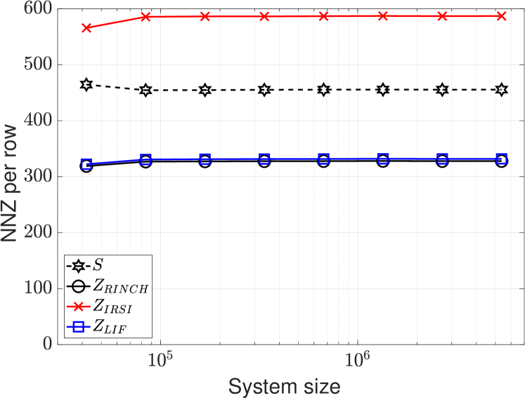
Figure 1 demonstrates how the algorithms behave with increasing system size in case of quasi-linear Glu-Ala helices. The curves represent scaling with 3 and 48 processes used. One can see that RINCH scales linearly, while LIF gives better time and scales better than linearly. IRSI shows similar scaling results, but works slower. One possible explanation of the scaling of LIF and IRSI is that before being saturated with work, processes have extra resources available. When saturated, they demonstrate a behaviour of the same type as RINCH shows. The number of non-zeros (NNZ) per row in stays almost constant, as well as in inverse factors computed with all three algorithms. IRSI provides the densest factors, while LIF and RINCH give approximately the same sparsity. Note that RINCH gains almost nothing from increasing the number of processes.
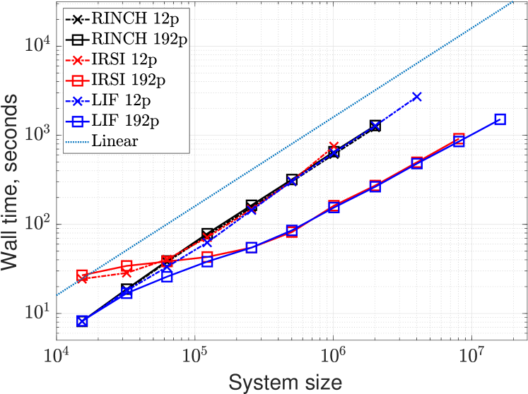
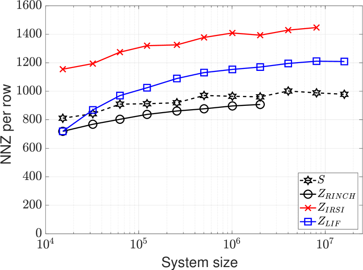
Figure 2 demonstrates how the algorithms behave with increasing system size in case of water clusters. Now the curves on the left plot represent scaling with 12 and 192 processes. One can observe linear scaling as the system size is increased. RINCH again shows no speedup when going from 12 to 192 processes. In case of 192 processes, LIF and IRSI scale slightly better than linearly, which indicates that the number of processes is too large and not all of them are saturated with work. Eventually the LIF and the IRSI algorithms arrive at very close timings. The number of nonzeros per row is no longer constant, it grows slowly with system size but flattens out for large systems [22]. Note that the RINCH algorithm was not able to handle the largest systems.
5.2 Strong scaling
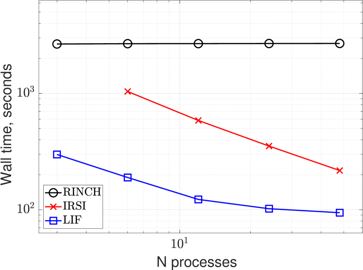
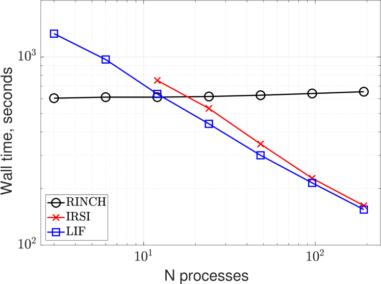
One can also fix the problem size and see how the execution time changes when the number of processes is increased. Figure 3 shows the scaling in the strong sense for the algorithms. As one can see, RINCH has an almost flat curve with no speedup. The other two algorithms exhibit strong scaling with similar behaviour, although the IRSI algorithm failed to handle small cases because of memory limitations.
5.3 Weak scaling, critical path length, and data movement
Due to the task-based nature of the Chunks and Tasks model and dynamic load balancing based on work stealing, it is very difficult to write down the exact formula for the speedup as a function of the number of processes involved. Therefore it is natural to use a different tool, like a critical path estimation, in order to predict the scaling in the weak sense. By weak scaling we mean how the parallel execution time changes when the workload increases in direct proportion to the number of processes.
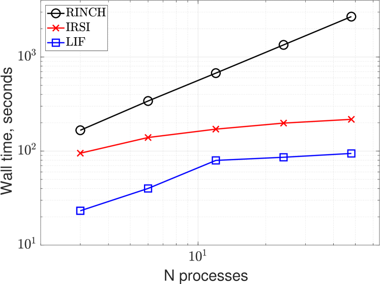
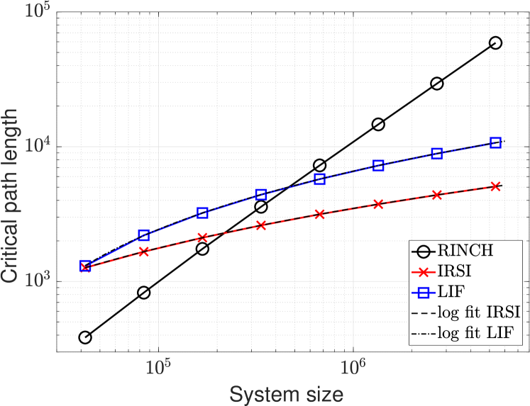
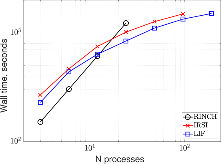
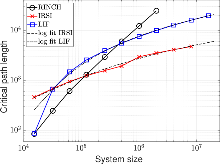
Figures 4 and 5 show how the algorithms scale in the weak sense and critical path lengths for Glu-Ala helices helices and water clusters, respectively. The figures show an approximate weak scaling since, strictly speaking, it is the number of basis functions per process and not the workload per process that is fixed as the number of processes is increased. Note however that the workload per process should approach a constant in the limit of large systems. The critical path length for the recursive inverse Cholesky algorithm increases linearly with system size as predicted in Section 3. The critical path lengths for iterative refinement with scaled identity and localized inverse factorization also agree with the theoretical results saying that the critical path lengths should increase as polynomials in . In all cases the wall times in these weak scaling tests are dominated by the execution of tasks, including associated communication, along the critical path. We noted that the coefficient in front of the term in the least squares fit was very small for both IRSI and LIF. For IRSI this is in perfect agreement with the theory, and for LIF it can be explained by matrix sparsity. Although the critical paths for the localized inverse factorization algorithm are typically longer than the critical paths for iterative refinement with scaled identity, the localized inverse factorization is faster. The reason is mainly that less communication is needed in the localized inverse factorization, as anticipated in the introduction.
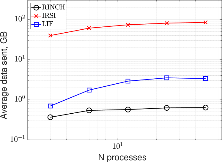
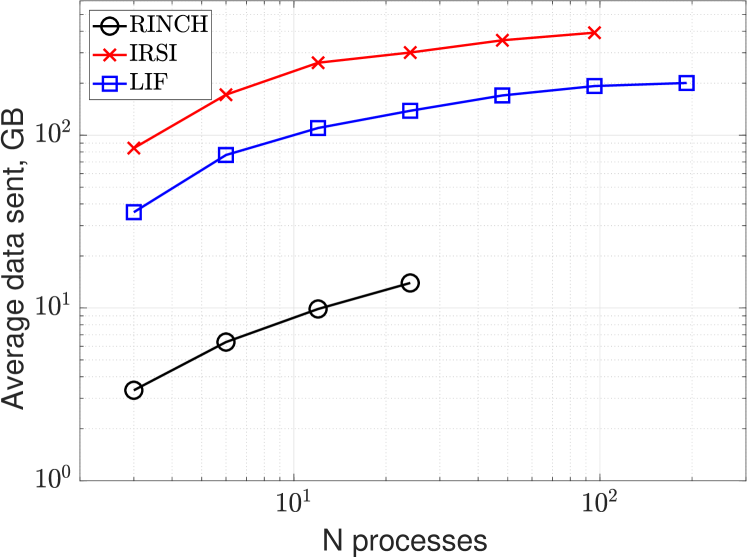
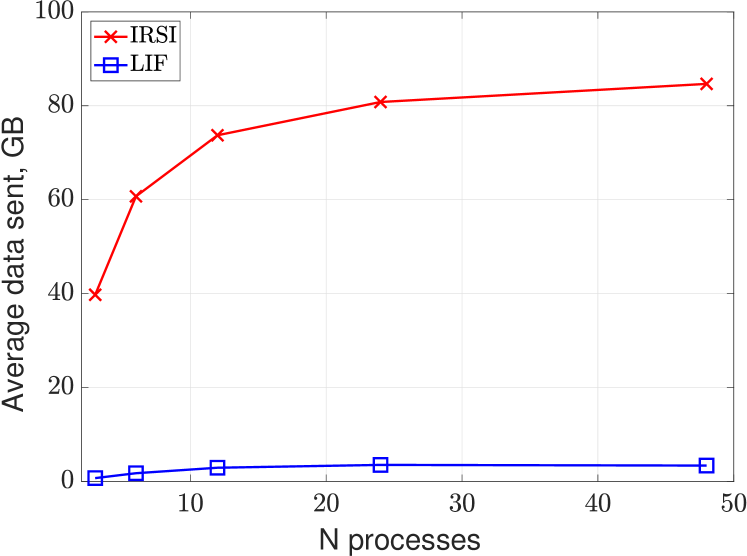
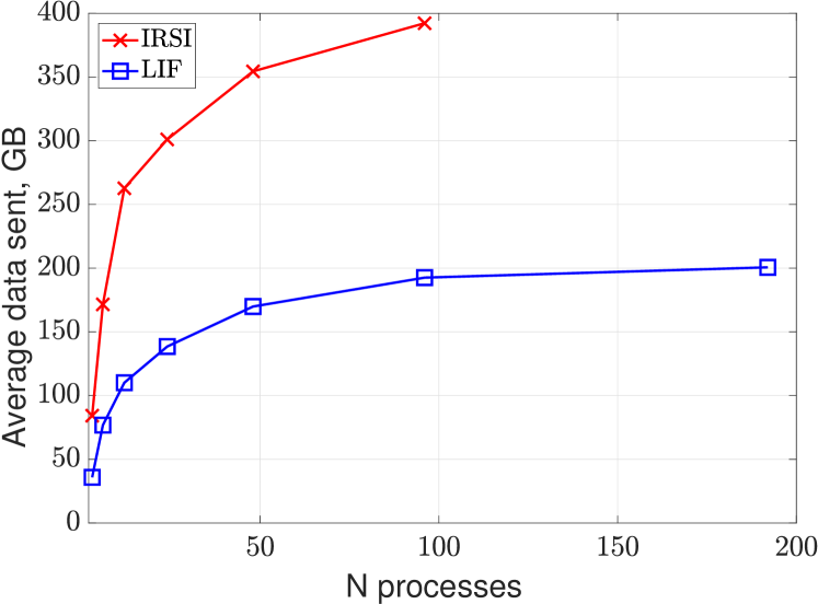
Figures 6 and 7 show the average amount of data sent per process for the weak scaling tests in Figures 4 and 5. The RINCH algorithm has the smallest average amount of data moved. This agrees with previous observations regarding the scaling in the weak and the strong sense and the critical path growth, since all the work is actually done by a single process only. So, there is not so much to move. In turn, the IRSI algorithm has the largest amount of data moved. Localized inverse factorization preforms better than IRSI. Although both IRSI and LIF are based on matrix-matrix multiplication, the localized computations used in LIF lead to a reduced amount of communication clearly visible in the plots.
Figure 7 shows the same dependency, but in linear-linear scale, and the advantage of LIF over IRSI is clearly visible in both cases. Note that for the LIF algorithm, the average amount of data moved becomes almost a constant for the system size increasing simultaneously with the number of processes at some point.
5.4 Factorization error
Table 1 demonstrates the difference between the algorithms in terms of factorization error We pick 2 particular cases, one for Glu-Ala helices and one for water clusters, b.f. stands for ”basis functions”, i.e. the system size. One can see that the RINCH algorithm provides the most accurate results in both cases. In turn, IRSI gives the least accurate results. Localized inverse factorization provides results of intermediate quality.
| RINCH | LIF | IRSI | |
|---|---|---|---|
| Glu-Ala, 5373954 b.f. | 0.00204 | 0.00259 | 0.02352 |
| Water clusters, 2006214 b.f. | 0.00603 | 0.00999 | 0.02628 |
6 Discussion and concluding remarks
The LIF algorithm can in principle be used by itself all the way down to single matrix elements. However, one may at any level in the hierarchy switch to some other algorithm to compute an inverse factor. In our numerical examples we switched to the recursive inverse Cholesky algorithm when the matrix size became smaller than or equal to 16384. In this way we combined the speed of the inverse Cholesky algorithm for small systems with the good parallel scaling and localization properties of the LIF algorithm. The advantage of LIF in this sense is clearly seen in Figure 2 where LIF is the most efficient algorithm for system sizes ranging over four orders of magnitude.
A drawback of IRSI is that it requires knowledge of at least some estimates to extremal eigenvalues to construct a starting guess. The convergence depends on the accuracy of those estimates. The extremal eigenvalues are not always cheap to calculate and in the present work we used the approximate scaling from [16] based on an estimate of the largest eigenvalue using the Gershgorin circle theorem. This approximate scaling resulted in convergence in all our numerical experiments, besides the calculations that were killed due to insufficient memory. However, one should be aware that the use of this scaling relies on an overestimation of the eigenvalue since an exact eigenvalue in (6) would lead to divergence.
An alternative not considered in this work is the family of multifrontal methods [12]. Similarly to the recursive and localized inverse factorization, multifrontal methods make use of a hierarchical decomposition of the matrix. In the multifrontal methods the matrix is seen as the adjacency matrix of a graph, which is split into two disconnected subgraphs using a vertex separator. This results in a 3 by 3 block division of the matrix. The 2 by 2 block division of the matrix in the localized inverse factorization can similarly be seen as the result of an edge separator of the graph. Since the two subgraphs in the multifrontal methods need to be disconnected, sparsity is needed to get parallelism. Without sparsity, there are no disconnected subgraphs. In LIF there is always parallelism, even if there is little or no sparsity. In the multifrontal methods explicit information about the sparsity pattern is needed to make the split. In LIF, any split leads to convergence, although good splits result in smaller initial factorization errors leading to faster convergence and/or more localized computations.
Finally we would like to stress that the present work is the first parallel implementation of the LIF algorithm and that previous implementations of IRSI made use of Cannon’s algorithm or SpSUMMA giving an unfavorable scaling in the weak sense. Therefore, to our best knowledge, our LIF and IRSI implementations using the Chunks and Tasks programming model are the first parallel inverse factorization implementations that achieve a weak scaling performance with the computational time increasing as a low order polynomial in .
7 Acknowledgements
Support from the Swedish national strategic e-science research program (eSSENCE) is gratefully acknowledged. Computational resources were provided by the Swedish National Infrastructure for Computing (SNIC) at the PDC Center for High Performance Computing at the KTH Royal Institute of Technology in Stockholm.
Appendix A Critical path length derivation for the RINCH algorithm
Let us first derive some useful expressions:
| (20) | ||||
| (21) | ||||
| (22) |
Since is a second order polynomial in , Then, (10) gives,
| (23) |
Appendix B Critical path length derivation for the RIF algorithm
Auxiliary formulas:
| (24) | ||||
| (25) |
Recall that is a second order polynomial in Then, (18) gives
| (26) |
References
- [1] An optimized BLAS library. http://www.openblas.net/. [Online; accessed December 12, 2018].
- [2] A. Azad, G. Ballard, A. Buluç, J. Demmel, L. Grigori, O. Schwartz, S. Toledo, and S. Williams, Exploiting multiple levels of parallelism in sparse matrix-matrix multiplication, SIAM J. Sci. Comput., 38 (2016), pp. C624–C651, https://doi.org/10.1137/15M104253X.
- [3] G. Ballard, A. Buluç, J. Demmel, L. Grigori, B. Lipshitz, O. Schwartz, and S. Toledo, Communication optimal parallel multiplication of sparse random matrices, in Proceedings of the Twenty-fifth Annual ACM Symposium on Parallelism in Algorithms and Architectures, SPAA ’13, New York, NY, USA, 2013, ACM, pp. 222–231.
- [4] M. Benzi, J. K. Cullum, and M. Tuma, Robust approximate inverse preconditioning for the conjugate gradient method, SIAM J. Sci. Comput., 22 (2000), pp. 1318–1332.
- [5] M. Benzi, R. Kouhia, and M. Tuma, Stabilized and block approximate inverse preconditioners for problems in solid and structural mechanics, Comput. Method. Appl. M., 190 (2001), pp. 6533–6554.
- [6] M. Benzi, C. D. Meyer, and M. Tuma, A sparse approximate inverse preconditioner for the conjugate gradient method, SIAM J. Sci. Comput., 17 (1996), pp. 1135–1149.
- [7] U. Borštnik, J. VandeVondele, V. Weber, and J. Hutter, Sparse matrix multiplication: The distributed block-compressed sparse row library, Parallel Comput., 40 (2014), pp. 47 – 58.
- [8] D. R. Bowler and T. Miyazaki, O(N) methods in electronic structure calculations, Rep. Prog. Phys., 75 (2012), p. 036503.
- [9] A. Buluç and J. R. Gilbert, Parallel sparse matrix-matrix multiplication and indexing: Implementation and experiments, SIAM J. Sci. Comput., 34 (2012), pp. C170–C191.
- [10] M. Challacombe, A simplified density matrix minimization for linear scaling self-consistent field theory, J. Chem. Phys., 110 (1999), pp. 2332–2342, https://doi.org/10.1063/1.477969.
- [11] W. Dawson and T. Nakajima, Massively parallel sparse matrix function calculations with NTPoly, Comput. Phys. Commun., 225 (2018), pp. 154 – 165.
- [12] I. S. Duff and J. K. Reid, The multifrontal solution of indefinite sparse symmetric linear equations, ACM T. Math. Software, 9 (1983), pp. 302–325.
- [13] S. A. Gershgorin, Über die Abgrenzung der Eigenwerte einer Matrix, Izv. Akad. Nauk S.S.S.R., 6 (1931), pp. 749–754.
- [14] N. J. Higham, Stable iterations for the matrix square root, Numer. Algorithms, 15 (1997), pp. 227–242.
- [15] N. J. Higham, Functions of matrices: theory and computation, SIAM, 2008.
- [16] B. Jansík, S. Høst, P. Jørgensen, J. Olsen, and T. Helgaker, Linear-scaling symmetric square-root decomposition of the overlap matrix, J. Chem. Phys., 126 (2007), p. 124104.
- [17] W. Kohn and L. J. Sham, Self-consistent equations including exchange and correlation effects, Phys. Rev., 140 (1965), p. A1133.
- [18] A. Kruchinina, E. Rudberg, and E. H. Rubensson, Parameterless stopping criteria for recursive density matrix expansions, J. Chem. Theory Comput., 12 (2016), pp. 5788–5802.
- [19] I. N. Levine, D. H. Busch, and H. Shull, Quantum chemistry, vol. 6, Pearson Prentice Hall Upper Saddle River, NJ, 2009.
- [20] J. M. Millam and G. E. Scuseria, Linear scaling conjugate gradient density matrix search as an alternative to diagonalization for first principles electronic structure calculations, J. Chem. Phys., 106 (1997), pp. 5569–5577, https://doi.org/10.1063/1.473579.
- [21] A. M. Niklasson, Iterative refinement method for the approximate factorization of a matrix inverse, Phys. Rev. B, 70 (2004), p. 193102.
- [22] E. H. Rubensson, A. G. Artemov, A. Kruchinina, and E. Rudberg, Localized inverse factorization, (2018), https://arxiv.org/abs/1812.04919.
- [23] E. H. Rubensson, N. Bock, E. Holmström, and A. M. Niklasson, Recursive inverse factorization, J. Chem. Phys., 128 (2008), p. 104105.
- [24] E. H. Rubensson and E. Rudberg, Chunks and Tasks: A programming model for parallelization of dynamic algorithms, Parallel Comput., 40 (2014), pp. 328–343, https://doi.org/10.1016/j.parco.2013.09.006.
- [25] E. H. Rubensson and E. Rudberg, Locality-aware parallel block-sparse matrix-matrix multiplication using the chunks and tasks programming model, Parallel Comput., 57 (2016), pp. 87–106.
- [26] E. H. Rubensson, E. Rudberg, and P. Sałek, A hierarchic sparse matrix data structure for large-scale Hartree-Fock/Kohn-Sham calculations, J. Comput. Chem., 28 (2007), pp. 2531–2537.
- [27] E. Rudberg, E. H. Rubensson, and P. Sałek, Kohn-Sham density functional theory electronic structure calculations with linearly scaling computational time and memory usage, J. Chem. Theory Comput., 7 (2011), pp. 340–350, https://doi.org/10.1021/ct100611z.
- [28] E. Rudberg, E. H. Rubensson, P. Sałek, and A. Kruchinina, Ergo: An open-source program for linear-scaling electronic structure calculations, SoftwareX, 7 (2018), pp. 107–111.
- [29] J. VandeVondele, U. Borštnik, and J. Hutter, Linear scaling self-consistent field calculations with millions of atoms in the condensed phase, J. Chem. Theory Comput., 8 (2012), pp. 3565–3573.
- [30] H. J. Xiang, J. Yang, J. G. Hou, and Q. Zhu, Linear scaling calculation of band edge states and doped semiconductors, J. Chem. Phys., 126 (2007), p. 244707, https://doi.org/10.1063/1.2746322.