A comparative study of estimation methods in quantum tomography
Abstract
As quantum tomography is becoming a key component of the quantum engineering toolbox, there is a need for a deeper understanding of the multitude of estimation methods available. Here we investigate and compare several such methods: maximum likelihood, least squares, generalised least squares, positive least squares, thresholded least squares and projected least squares. The common thread of the analysis is that each estimator projects the measurement data onto a parameter space with respect to a specific metric, thus allowing us to study the relationships between different estimators.
The asymptotic behaviour of the least squares and the projected least squares estimators is studied in detail for the case of the covariant measurement and a family of states of varying ranks. This gives insight into the rank-dependent risk reduction for the projected estimator, and uncovers an interesting non-monotonic behaviour of the Bures risk. These asymptotic results complement recent non-asymptotic concentration bounds of [36] which point to strong optimality properties, and high computational efficiency of the projected linear estimators.
To illustrate the theoretical methods we present results of an extensive simulation study. An app running the different estimators has been made available online.
1 Introduction
The problem of estimating unknown parameters of quantum systems has been at the forefront of early investigations into the statistical nature of quantum information [13, 43, 42, 79, 16]. Traditionally, key research topics have been the design of optimal measurements and estimation procedures [56, 77, 21, 31, 47, 8, 9, 41, 9], and theoretical aspects of quantum Fisher information and asymptotic estimation [11, 28, 57, 41, 6, 62, 45, 30], see also the monographs [59, 52, 40].
More recently, quantum tomography has become a crucial validation tool current quantum technology applications [38, 58, 29, 67]. The experimental challenges have stimulated research in new directions such as compressed sensing [35, 54, 27, 70, 20, 5, 3], estimation of permutationally invariant states [73], adaptive and selflearning tomography [55, 34, 60, 26, 39, 63], incomplete tomography [74], minimax bounds [25, 4], Bayesian estimation [15, 33], and confidence regions [7, 18, 71, 24, 53]. Since ‘full tomography’ becomes impossible for systems composed of even a moderate number of qubits, research has focused on the estimation of states which belong to smaller dimensional models which nevertheless capture relevant physical properties, such as low rank states [48, 17, 37, 49, 36] and matrix product states [20, 12, 50].
In this paper we analyse and compare several estimation methods for fixed (non-adaptive) measurement designs, with a focus on risks (mean errors) for different loss functions, asymptotic theory, relationships between estimators and low rank behaviour. The measurement scenarios include repeated measurements with respect to Pauli bases (as customary in multiple qubits experiments), random bases measurements, and the covariant measurement. The loss functions are given by the Frobenius, trace-norm, operator-norm, Bures and Hellinger distances. Each section deals with one class of estimators and the results of a comparative simulations study are presented at the end of the paper. While most estimators have been previously considered in the literature, our aim is to investigate them from a common perspective, as projections of data onto the parameter space. Another aim is to understand and quantify the reduction in statistical error between an unconstrained estimator such as least squares, and an estimator which take into account the physical properties of the parameter space, such as the projected least squares estimator. Among the original results, we derive the asymptotic error rates of these estimators on a class of low rank states in the covariant measurement scenario. Finally, we discuss the computational efficiency of different methods.
Below we summarise the paper using Figure 1 for illustration. A measurement on -dimensional system is a positive affine map from the convex set of states (constrained parameter space) onto the space of outcome probabilities , where is the number outcomes. The image of the set of trace-one selfadjoint matrices (unconstrained parameter space) is a hyperplane of , which contains . For informationally complete measurements the map is injective and we can identify all matrix estimators (whether positive or not) with their images in .

In section 3 we review the use of Fisher information in asymptotic normality theory and discuss to what extent it is applicable to the study of the maximum likelihood (ML) estimator in quantum tomography [10, 14, 66, 75]. We distinguish between two ML estimators: the unconstrained estimator , and the ‘physical’ estimator . The former is the maximiser of the likelihood, seen as a function over , and may not be a density matrix. The latter performs the same optimisation but restricted to the physical space of density matrices . For large sample size, the unconstrained estimator is asymptotically normal, while the constrained estimator is equal to its projection onto with respect to the metric defined by the classical Fisher information [66].
In section 4 we analyse the least squares (LS) estimator . This exploits the linear dependence between probabilities and states which translates into a linear regression problem
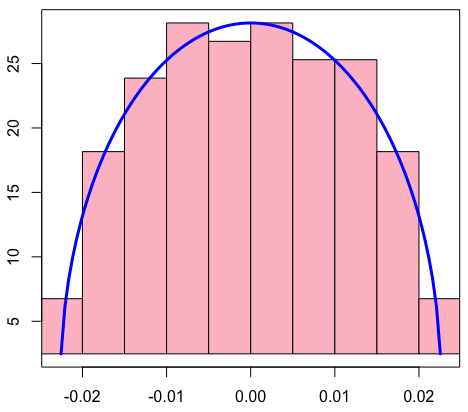
where denotes the vector of observed frequencies of measurement outcomes, is a fixed measurement design matrix, is a vectorisation of the unknown state , and is the statistical noise. The LS estimator minimises the prediction error over all vectors , and is the simplest and fastest estimator to compute. However, LS is significantly less accurate than ML, especially for low rank states and does not produce a physical state. Nevertheless, the LS has been the focus of recent investigations [17, 72, 36] as a first step towards more accurate estimators. Here we review some of the non-asymptotic concentration bounds for the operator-norm error of the LS estimator. We then study the asymptotic properties of the LS estimator in the context of covariant measurements, and rank states with equal non-zero eigenvalues. By exploiting the symmetry of the measurement we compute the explicit expression of the risk with respect to the Frobenius distance. Furthermore, we show that for large , the eigenvalues of the ‘error matrix’ are approximately distributed according to the Wigner semicircle law on the interval , cf. Figure 2. This provides the asymptotic estimates of the operator-norm, and the trace-norm errors of and respectively , which complement the non-asymptotic bounds of [36].
In section 5 we discuss the generalised least squares (GLS) estimator. Unlike the LS estimator which minimises the prediction error, the GLS aims to optimise the estimation error, e.g. and needs to take into account the covariance matrix of the multinomial noise . We show that for large samplesize , the GLS estimator is asymptotically normal and is equivalent to the uML estimator.
Section 6 reviews the thresholded least squares (TLS) estimator proposed in [17]. This is obtained by projecting the LS estimator onto the set of states whose non-zero eigenvalues are above a certain ‘noise level’ chosen in a data-driven fashion. The projection can be computed efficiently in terms of the eigenvalues of the LS estimator, and the truncation leads to significant error reduction for low rank states. In practice, an additional improvement is achieved by using the GLS estimator as starting point.
Section 7 discusses the positive least squares (posLS) estimator which optimises the prediction error over the physical space of density matrices, rather than over the selfadjoint matrices as is the case for the LS estimator [46]. This leads to higher accuracy, but its computational complexity is similar to that of ML. However, in the case of the covariant measurements we find that posLS is equivalent to the projected least squares estimator discussed below, which can be computed efficiently. By restricting the GLS optimisation over density matrices we obtain the positive generalised least squares estimator (posGLS), which is shown to be asymptotically equivalent to the ML estimator.
Section 8 deals with the projected least squares (PLS) estimator. This is obtained by projecting the LS estimator onto the space of density matrices with respect to the Frobenius distance [72, 36]. It is faster than TLS, and has similar statistical properties. In [36] is was shown that the PLS estimator satisfies rank-dependent concentration bounds and its trace-norm error scales as for a broad class of 2-design measurements including mutually unbiased bases, stabiliser states, and symmetric informationally complete measurements, and as for Pauli bases measurements. In this paper we focus on the asymptotic behaviour of the PLS estimator in the case of covariant measurements. Inspired by the techniques developed in [66] we show how the random matrix properties of the LS can be used to derive the asymptotic Frobenius and Bures risks of the PLS estimator for low rank states and large dimension and samplesize . In particular we uncover an interesting behaviour of the Bures risk which (unlike the Frobenius or the trace norm risks) increases steeply with rank for low rank states and then decreases towards full rank, cf. Figure 3.
Section 9 presents the results of a comparative simulations study of the proposed estimators. We simulated data for a range of states of 3 and 4 atoms of different ranks, with different samplesizes, and measurement setups. For each choice we produced 100 datasets in order to estimate risks of different estimators. The measurements are chosen to be either Pauli bases measurements (as standard in ion trap experiments) or random basis measurements. The different estimators and their risks corresponding to Frobenius, Bures, Hellinger, and trace-norm distances were computed and the results are illustrated and discussed, cf. Figures 4, 5, 6, 7, 8, 9, 10, and 11. A complete set of simulation results available online via an interactive Rshiny application at https://rudhacharya.shinyapps.io/plots/. We also created an online estimation app which computes the key estimators for a range of states of certain characteristics, or user uploaded states. This is available at https://shiny.maths.nottingham.ac.uk/shiny/qt_dashboard/.
2 Quantum tomography
In quantum tomography, the aim is to estimate an unknown state from outcomes of measurements performed on an ensemble of identical prepared systems. Although a large part of our theoretical considerations hold in a general setting, we choose to formulate the tomography problem in the specific context of a system consisting of multiple qubits and projective measurements with respect to several bases. This keeps the discussion closer to realistic experimental procedures, and facilitates the understanding of our simulation results.
We consider composite systems consisting of qubits, with associated Hilbert space , where . The state belongs to the space of density matrices . In our analysis we will distinguish between the constrained parameter space whose elements are trace-one positive matrices, and the unconstrained parameter space consisting of trace-one selfadjoint matrices. This will allow us to consider procedure which produce constrained, or unconstrained estimators.
The measurement strategies consist of performing standard, von Neumann projective measurements with respect to a number of orthonormal bases (ONB), which are chosen deterministically or randomly. In particular, we focus on two scenarios: Pauli basis measurements and measurements that are drawn randomly from the uniform measure over all ONBs. While the former setup is commonly employed in experiments [38], the latter is less restrictive, more amenable to theoretical analysis, and can serve as a benchmark for current experiments. We also consider covariant measurements in the context of the asymptotic theory of the least squares and respectively projected least squares estimators in sections 4.3 and 8.1, and refer to these for further details.
In the Pauli bases setup, one measures an arbitrary Pauli observable , or on each of the ions simultaneously. Therefore, each measurement is labelled by a sequence , and there are possible measurement bases. Such a measurement produces a outcome from each ion, and we let be the full record of outcomes from all the ions. The probability of obtaining a particular outcome is given by , where is the one-dimensional projection onto the tensor product of eigenvectors of Pauli matrices
More generally, the measurement design is defined by a collection of ONBs, which may be chosen deterministically or randomly. For each setting , independent measurements are performed on identical copies of the state, and the counts are recorded, where is the number of times the outcome is observed when measuring in setting . The total number of quantum samples is therefore . The resulting dataset is a table whose columns are independent and contain all the counts in a given setting. Its probability is given by the product of multinomials
| (1) |
Our goal is to statistically reconstruct the density matrix from the counts dataset . This can be seen as a statistical inverse problem of reversing the measurement map
in the sense that given a sample from , one would like to produce an estimator which is close to with respect to some meaningful distance measure. The next section lists several figures of merit considered here.
2.1 Error functions
| Error function | Definition |
|---|---|
| Frobenius norm squared | |
| Trace norm | |
| Operator norm | |
| Bures distance | |
| Hellinger distance |
Let us denote the risk or mean error of an estimator as , where represents a particular error function. In our theoretical analysis and simulations study we estimate the risk for several choices of the error function , which are tabulated in Table 1. Note that the Bures distance is defined only over the space of density matrices, and therefore applies only in the case where the estimators are density matrices. The classical analogue of the Bures distance is the Hellinger distance between two probability distributions. Here we consider the Hellinger distance between the eigenvalues of the true state and those of the estimator , seen as probability distributions. Later on we will show that the behaviour of the Bures distance error is strongly correlated with that of the squared Hellinger distance error.
3 Fisher information, asymptotic normality and maximum likelihood
The maximum likelihood (ML) estimator is one of the most commonly used and well understood statistical tools with a universal range of applicability. Before considering its use in quantum tomography, we briefly review some of the key concepts and results related to the ML estimator and its asymptotic behaviour [51, 78]. Consider the scenario in which we are given independent samples from a discrete probability distribution over a countable set ; the probability distribution is assumed to depend smoothly on an unknown parameter which belongs to an open subset of . The likelihood of the dataset is . The ML estimator is the point in where the likelihood of the observed data attains its maximum value
The likelihood can be expressed in terms of the empirical distribution of the data which collects the frequencies of different outcomes in . Indeed the log-likelihood can be written as (cf. (1))
where relative entropy (Kullback-Leibler divergence), and do not depend on . The ML estimator is thus the closest point to with respect to the relative entropy
Asymptotics. The appeal of the ML estimator lies in part in its asymptotic optimality properties. For large enough sample sizes , a central limit behaviour emerges and the ML estimator becomes normally distributed around the true parameter, with a variance shrinking at the rate
| (2) |
The convergence above holds in distribution as and the limit is a centred Gaussian distribution with covariance given by the inverse of the Fisher information matrix. The latter is a positive matrix
which encapsulates how informative a single sample from is about . The limiting covariance is equal to the lower bound appearing in the the Cramér-Rao inequality for unbiased estimators. Estimators which satisfy equation (2) are called efficient and statistical theory shows that one cannot improve on their asymptotic accuracy, except on a measure zero set of the parameter space [51]. In particular if is a locally quadratic (positive) loss function on ,
then the risk of the MLE satisfies
It is important to note that the asymptotic normality property (2) relies on the smoothness of the model and the fact that is an interior point of the parameter space . For large the ML estimator lies (with high probability) within in a small neighbourhood of of size , and the parameter space looks like for all practical purposes. However, when has a boundary, the ML estimator will not be asymptotically normal for parameters lying on the boundary, and one needs to analyse such models more carefully. This is the case in quantum tomography, when the unknown state is not full-rank and therefore lies on the boundary of , or is so close to the boundary that the asymptotic theory will kick in only for sample sizes that are much larger than those obtained in real experiments.
3.1 The maximum likelihood estimator in quantum tomography
We will now discuss in more detail the properties of the MLE in the specific case of quantum tomography. Given the measurement data encoded in the dataset , the MLE is defined as the maximum of over . By passing to log-likelihood and discarding the constant factorial terms in (1), we obtain the following form of the estimator
| (3) |
where are the empirical frequencies of the data. The MLE is commonly used in quantum tomography [10, 14, 44, 32], and several implementation methods have been proposed including Hradil’s iterative algorithm [64]. Our specific implementation uses the CVX package for disciplined convex programming on MATLAB [2]. The general asymptotic theory guarantees that the ML estimator is asymptotically normal for full rank states, i.e. the interior of . To get more insight into the general asymptotic behaviour for a given state , we will choose a local parametrisation defined in terms of the matrix elements of with respect to its eigenbasis. Let be the eigenvalues of a full-rank state . Then any neighbouring state can be written as
where is trace zero matrix which is completely parametrised by
| (4) | ||||
The ML estimator has parameter which is normally distributed around with covariance where the Fisher information is the average of the individual informations for different sets
| (5) |
In particular, for any locally quadratic loss function (e.g. Frobenius distance, or Bures distance) with weight matrix , the associated risk has the asymptotic behaviour
| (6) |
Now, let us assume that the unknown state is on the boundary of , and more precisely belongs to the space of rank states , for a fixed and known rank . In its own eigenbasis, is the diagonal matrix of eigenvalues , and any sufficiently close state is uniquely determined by its matrix elements in the first rows (or columns). Intuitively this can be understood by noting that any rank- state in the neighbourhood of can be obtained by perturbing the eigenvalues and performing a small rotation of the eigenbasis; in the first order of approximations these transformation leave the lower-right corner unchanged so
| (7) |
where . We therefore choose the (local) parametrisation where only the matrix elements of and enter the parameter . For this model, any rank- state corresponds to an interior point of the parameter space , and consequently the ML estimator obeys the asymptotic normality theory described above.
However, if the rank of is not known in advance, then the diagonal block of needs to be included in the model in order to describe neighbouring states of higher rank. As is a state, the block is a positive matrix, and therefore its matrix elements are constrained. This complicates the analysis of the likelihood function, and invalidates the asymptotic normality of the ML estimator.
What should be the theory replacing asymptotic normality ? At the moment there isn’t a complete answer to this question, but some important progress has been made in [66]. Following this work and [17], it is instructive to study an extended, ‘non-physical’ model in which the positivity requirement is dropped and (locally around ) the parameter space is taken to be that of selfadjoint matrices of trace-one . Therefore, the ‘unphysical’ parameter consists of the matrix elements of the blocks (except one diagonal element due to normalisation), with given by equation (7). We now make the ‘mild’ assumption that for all pairs ; indeed this condition is satisfied for ‘generic’ states but fails for states whose support is orthogonal to some of the measurement basis vectors. Under this assumption, we find that locally around , we can define a statistical model given by bona-fide probability distributions We can therefore define the unconstrained maximum likelihood (uML) estimator as in equation (3) where the optimisation is performed over the unconstrained local neighbourhood of , rather than over the space of states . Since is on the boundary of , the probability that falls outside the state space is significant and does not vanish in the asymptotic limit. In this case, does not coincide with the ‘constrained’ or regular ML estimator . In fact, each of them can be seen as the projection with respect to the relative entropy distance of the empirical distribution onto the sets of probabilities and respectively , where is the measurement map.
Asymptotics. Since corresponds to an interior point of the unconstrained parameter space, the general asymptotic normality theory applies again. In particular, the uML estimator is normally distributed around with variance , where is the Fisher information (5) computed with respect to the unconstrained parametrisation. Moreover by Taylor expanding the log-likelihood function around the , and using the fact the the first derivative vanishes at this point, we obtain the second order approximation
| (8) |
This implies tht for large , the ML estimator is the projection of onto with respect to the quadratic distance determined by the Fisher information
| (9) |
Moreover, the probability distribution of the MLE is obtained by projecting the Gaussian distribution corresponding to , onto . Although the projection can be computed efficiently using convex optimisation, finding a general characterisation of the resulting distribution seems to be a challenging problem [71]. Nevertheless, [66] shows that the problem is tractable in those cases where the metric is (approximately) isotropic, so that random matrix results such as the emergence of Wigner semicircle law can be used to treat the asymptotic theory. In section 8.1 we will use these ideas to study the asymptotic behaviour of the projected least squares estimator.
4 The least squares estimator
The least squares (LS) estimator [63, 17] is based on the observation that the outcome probabilities depend linearly on the state . Let
| (10) |
be the decomposition with respect to an orthonormal basis of consisting of selfadjoint matrices , and the corresponding vectorisation. Then the probabilities can be expressed as
where is a fixed matrix depending on the measurement and the chosen vectorisation. In an experimental setup we do not have access to the true probability vector. Instead from the dataset of counts, we can compute the empirical probabilities , whose expectations are . Replacing probabilities vector with empirical frequencies
| (11) |
where is a mean zero vector of statistical noise. The noise distribution is irrelevant for the definition of the LS estimator, but we will return to this when discussing its error, and the generalised least squares estimator.
The least squares solution to the above system of equations is defined as the minimiser of the following optimisation problem
| (12) |
and has the explicit form . The final estimate of the density matrix is then constructed from the estimated parameter vector using equation (10). We note that the least squares estimator produces a state estimate that is not necessarily a density matrix.
Least squares as a projection. Let be the map associated to the measurement, and let be the ‘probability distribution’ corresponding to the LS estimator. This belongs to the hyperplane which contains the convex set of probabilities . The LS estimator (12) can then be interpreted as the projection of the frequency vector onto with respect to the Euclidian distance in .
4.1 Least squares as inversion of a measure-and-prepare channel
The LS estimator was introduced above by choosing a particular vectorisation of the density matrix. While this is useful for numerical implementations, the disadvantage is that one loses the physical interpretation of the quantum state and the measurement map. Conceptually, it is useful to define the LS estimator in a “coordinate free” way which can be interpreted as the inversion of a certain measure-and-prepare map associated to the measurement [36]. Let be the quantum channel
which is the composition of the measurement with collection of bases , and the preparation map where the pure state is prepared for each outcome of the measurement in basis . If is represented in its vectorised form, then the map is given by the matrix . On the other hand, the preparation map has matrix , so that the LS estimator can be expressed as
| (13) |
From this expression we see immediately that as consequence of the fact that is a probability distribution and is trace preserving. Additionally, we note the the accuracy of the LS estimator is linked to the properties of the channel . In particular, in the case of Pauli measurements the channel is given by a tensor product of qubit depolarising channels [17, 36]
On the other hand, the measurements corresponding to the class of 2-designs (which includes covariant measurements, mutually unbiased bases, stabiliser states, symmetric informationally complete measurements) have associated channel given by [36]
4.2 Concentration bounds and asymptotic behaviour of the LS
For more insight into the structure of the LS estimator let us unpack equation (13) and note that can be written as an average of independent, identically distributed matrices with
| (14) |
where are the outcomes of the measurements with respect to setting .
In this form, the LS estimator is amenable to non-asymptotic matrix concentration techniques, as well as asymptotic normality theory. The following result [36] was obtained by applying matrix Bernstein inequalities [76] and provides a non-asymptotic confidence bound for LS with respect to the operator norm distance, see also [17].
Theorem 4.1:
Let be the LS estimator of for a dataset consisting of samples. Then
where for design measurements and for Pauli measurements.
The theorem provides upper bounds for risks with respect to commonly used loss functions such as the Frobenius distance (norm-two squared) and the trace-norm distance, see also [72] for related results. Indeed using the basic inequalities and we obtain the upper bounds
| (15) |
for the 2-design measurements and
| (16) |
for the Pauli basis measurement, where are a numerical constants. Moreover, in [36] it was shown that the log factor in (15) can be removed when we deal with covariant measurements. On the other hand, in section 3 we have shown that for the maximally mixed state, the optimal convergence rate for the Frobenius distance is of the order ; this means that the upper bound (15) cannot be improved, when seen as a uniform bound over all states. However, this leaves open the possibility that special classes of states can be estimated with higher accuracy that that provided by the LS estimator. Indeed, we will see that simple modifications of the LS estimator which take into account the positivity of the unknown state can significantly reduce the estimation errors for low rank states.
Asymptotics. Thanks to its simplicity, the LS estimator has a tractable asymptotic theory. As in the case of the concentration Theorem 4.1 the key point is that the error is a sum of independent, identically distributed matrices given by equation (14). In the limit of large each matrix element of has a Gaussian distribution; in terms of the vectorised form we have the Central Limit for
where is the (renormalised) covariance of the noise . Due to the independent structure of the measurement settings, the latter has a non-trivial block diagonal form with blocks corresponding to the different settings
| (17) |
This allows us in principle to compute the asymptotic risk of an arbitrary quadratic loss function with weight matrix (such as the Frobenius distance) as
Since is a vector of frequencies, it must satisfy normalisation constraints, which is reflected in the fact each block is singular, with zero eigenvector . Consequently, the covariance matrix is singular with the zero eigenvector corresponding to the trace which is a fixed parameter. We will come back to this when discussing the generalised least squares estimator.
4.3 Asymptotic theory of LS for covariant measurements
While asymptotic normality tells us that the estimator lies in an ellipsoid centred at , it treats the estimator as a vector rather that as a matrix. For instance, it does not immediately provide an asymptotic theory for the operator norm error . Random matrix theory provides us with other asymptotic results which take into account the matrix structure of the estimator. To explore this avenue we will make a simplifying assumption and place ourselves in the scenario of covariant measurements. The outcome of such a measurement is a one dimensional projection and the corresponding positive operator valued measure is
| (18) |
where is the uniform measure over the space of one dimensional projections; the latter is the measure induced by the Haar measure over the unitaries via the action . An alternative way of obtaining a measurement sample is to choose a random basis and perform a measurement with respect to the chosen basis.
In this setup, the channel is given by [36]
and the LS estimator given by equation (14) can be written as
where are the independent outcomes of measurements.
We will be particularly interested in the behaviour of the LS estimator for low rank states, as well as states close to the maximally mixed one. Due to covariance it suffices to choose states which are diagonal in the standard basis , and for simplicity we will restrict ourselves to rank-r states with equal eigenvalues . As in section 3.1 we write the LS estimator as
| (19) |
where are block matrices of mean zero, and is the identity block. We will deal with each block separately.
Block C. By covariance, the distribution of the block is invariant under unitary transformations in . As the LS estimator is unbiased, the matrix elements of are centred. The off-diagonal elements have real and imaginary parts with variances equal to
with
where we have written for and replaced the integration over projections with that over unitaries; the integral was then evaluated using Weingarten formulas [19]. Similarly, the variance and covariance of the diagonal elements are
and all off-diagonal elements (of all blocks ) have zero covariance with other matrix elements. By the Central Limit Theorem, in the limit of large , the off-diagonal elements of become normally distributed and independent of all other elements. On the other hand, as the covariance of diagonal elements is non-zero, they converge to correlated Gaussian variables. However, if we also take the limit of large we find that the covariance of the diagonal elements vanishes and the matrix is distributed approximately as the Gaussian unitary ensemble (GUE). Universality results for random matrices [65] imply that the empirical distribution of the eigenvalues of converges weakly to Wigner’s semicircle law on the interval , whose probability density is
| (20) |
Indeed, panel a) of Figure 2 shows a good match between the histogram of the eigenvalues of the error block for a rank-one state of atoms and samples, and the corresponding Wigner distribution.
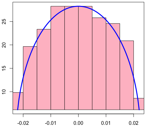
Block A. Let us consider now block of equation (19). For the same symmetry reasons, its off-diagonal elements (when ) have real and imaginary parts with variance
with
where all indices are different. The diagonal elements have variance
while the covariance of the diagonal elements is
We note that for small the diagonal elements do not become independent when and are large. However, if we also take to be large, the covariance vanishes, as in the case of the block. By the same argument, the distribution of the eigenvalues of converges to the Wigner semicircle law (20). This is illustrated in the right panel of Figure 2, for the case of the totally mixed state of atoms.
Block B. The elements of block B have variances equal to
with and
Eigenvalues distribution of the LS estimator. To better understand the LS estimator, it is instructive to study the distribution of its eigenvalues. This will also be used in the study of the projected least squares estimator furher on. Assuming is large, we note that can be written as
| (21) |
where
This means that in the leading order in the set of eigenvalues of is the union of those of and . In the case of large and small rank , the first group of eigenvalues are small fluctuations of size around ; in particular these eigenvalues are positive with high probability; the second group of eigenvalues are distributed according to the Wigner law, and have maximum absolute value approximately equal to , and roughly half of them will be negative.
We can now evaluate the asymptotic risk of the LS estimator with respect to the chosen loss functions.
Frobenius risk. For the Frobenius distance, the asymptotic mean square error is
In particular, the leading contribution to the Frobenius risk is , and the dependence with is weak. As illustrated in panels a) and b) of Figure 3 the theoretical prediction match the simulation results for 5 and 6 atom states.
Operator norm risk. The operator-norm error of the LS estimator is
Above we found that the entries of become independent in the limit of large , except for correlations between the diagonal elements which vanish if we additionally take the limit of large . Moreover, the variances of the elements in the block and the off-diagonal elements of differ from those of the off-diagonal elements of by factors and respectively . Therefore, the error block matrix as a whole is not distributed according to GUE ensemble. However, the universality of the Wigner semicircle law, the limit holds not only for highly symmetric ensembles like GUE but also for ‘small’ perturbations of this ensemble, e.g. random matrices with independent entries, whose variances do not deviate too much from a fixed value [23]. In particular for low rank , the total size of the blocks is of the order which is much smaller than than the size of . Therefore, the asymptotic behaviour of the error matrix is determined by that of and its spectrum converges to the Wigner law in the limit of large sample size and large dimension. In particular, the leading contribution to the norm error for low rank states is . A similar situation occurs for high rank states where the dominant variances are provided by the block .
Indeed simulations for a pure and the fully mixed state of atoms with samples gave norm errors and respectively , while the above theoretical prediction is . Further simulation results for and atoms states of different ranks show a good match with the above estimate.
Trace norm risk. As in the case of the operator norm, the trace norm error can be estimated thanks to the fact that the eigenvalues of error matrix follow an approximate Wigner semicircle distribution. Using
we find that for low rank, or close to full rank states, the leading contribution to is . This rate agrees with the upper bound in equation (15), but provides an exact asymptotic constant for this rate. Indeed simulations with a pure and maximally mixed states of atoms and samples gave norm-one errors of and respectively while the theoretical prediction is .
5 Generalised least squares estimator
Consider the generic linear regression problem
| (22) |
with and unknown vector, a vector of observations and the ‘noise’ term with fixed and known covariance matrix , which is assumed to be strictly positive. While the LS estimator is optimal in the sense of minimising the prediction error , this is not the case when considering an estimation error e.g. the mean square error , unless the covariance matrix is proportional to the identity. To recover the ‘equal noise’ situation we multiply equation (22) from the left by , to obtain
The LS estimator of the last regression equation has the smallest covariance matrix among linear unbiased estimators
This is called the generalised least squares (GLS) estimator. when the noise distribution is Gaussian, the GLS estimator coincides with the MLE. In the i.i.d. setting where samples are available, the GLS estimator is asymptotically normal and efficient
| (23) |
GLS as a projection. Similarly to the LS estimator we consider the image of the GLS estimator . Then is the projection of the data onto the subspace with respect to the covariance-dependent metric
GLS for tomography. Let us return now to the tomography regression problem of the form given by equation (11). While the LS estimator is optimal in the sense of equation (12), in general it is not optimal in the estimation sense for any locally quadratic distance function. To remedy this we would like to construct a corresponding generalised least square estimator to take into account the nontrivial form of the noise covariance matrix given by equation (17). However, there are two issues which prevent us from directly applying the GLS methodology to the tomography data. The first is that is unknown since it depends on the true probabilities, and therefore on the unknown state . We therefore propose to use an estimate of the covariance matrix instead. We describe the computation of this estimate in Appendix A.2. The second difficulty is that is a singular matrix due the constraint for each setting . This means that for each setting the vector is a zero eigenvector for and one should work within the orthogonal complement of . This can be achieved by choosing a block-diagonal isometry such that each block satisfies , and defining the new ‘frequencies’ vector with settings components . Similarly, we can also remove the trace-one constraint for states by choosing the vectorisation (10) such that the last basis element is . In this case the state is uniquely determined by the free parameters . If we denote by the isometric embedding with respect to the standard basis, then is the truncated vector of free parameters for .
The regression problem can now be written in terms of the ‘tilde’ vectors and matrices
where and has covariance matrix which is non-singular. We can now apply the GLS methodology and define the estimator as
where is the (non-singular) estimated covariance matrix. We denote as estimate of the density matrix constructed from its vectorised form . For future use, let us denote the map , so that .
5.1 Asymptotic theory of GLS
What are the asymptotic properties of ? For large , the noise distribution becomes Gaussian, and the covariance estimator converges to the actual covariance. The estimator becomes asymptotically normal as
| (24) |
which means that the corresponding asymptotic average Fisher information per sample is . In appendix A.1 we show that coincides with the Fisher information defined as in equation (5) for the parametrisation . This equality implies that the error rates of the GLS estimator have the same asymptotic behaviour as those of the uML estimator, and both estimators satisfy asymptotic normality. In fact one can make the stronger statement that the two estimators are asymptotically close to each other.
Equivalence of GLS and uML. As stated above, the GLS can be interpreted as the projection of the data onto the image of in with respect to the metric
On the other hand, in section 3.1 we showed that for large , we can define the uML estimator as the projection of onto the hyperplane , with respect to the relative entropy distance. Since in the first order of approximation the relative entropy is given by the quadratic form , the two projections become identical in the asymptotic limit.
6 Thresholded least squares estimator
The LS estimator (as well as GLS) suffers from the disadvantage that it does not necessarily produce a density matrix, i.e, a positive semi-definite estimate of trace one. While the significant eigenvalues can be estimated reasonably well with enough data, the LS estimator will typically have negative eigenvalues corresponding to small or zero eigenvalues of the true state. The thresholded least squares estimator (TLS) proposed in [17], improves the LS estimator by selecting the state which is the closest in Frobenius norm to and whose non-zero eigenvalues are above a certain threshold , i.e.
with the set of density matrices with spectrum in . The choice of the statistical noise threshold is informed by the accuracy of the LS estimate, and a theoretical and a ‘data-driven’ choices for this threshold are detailed in [17], see also [69, 22]. In practice it is found that estimator’s performance improves if the threshold is allowed to be ‘data-driven’, by using cross-validation to choose the optimal value of the threshold, see Appendix A.2.
It turns out that computing is very efficient and can be easily implemented. Let
be the spectral decomposition of where we assume that the eigenvalues are sorted in descending order . The thresholded estimator
has the same eigenvectors as , and its eigenvalues can be computed in terms of as summarised in Algorithm 1.
for do
In words, the algorithm checks if the smallest eigenvalue of is above the noise threshold, and if it is then ( note that by construction , so there is no need to renormalise the LS estimator). On the other hand if the smallest eigenvalue is below the threshold, it is set to zero and the remaining eigenvalues are suitably shifted accordingly so that their sum is equal to one. The final estimate is constructed by replacing the eigenvalues of with these thresholded eigenvalues . The theoretical properties of the TLS estimator are presented in [17] and are similar to those of the projected least squares estimator which is discussed in more detail below.
6.1 Thresholded Generalised Least Squares Estimator (TGLS)
This estimator is obtained by using the GLS estimate instead of the LS estimate as a starting point for the thresholding procedure. The constant for thresholding is chosen in the same way by using cross-validation. The advantage of TGLS is that it starts from a more accurate estimator than LS, which leads to smaller errors compared to TLS. The price to pay is that it is somewhat more involved computationally, although still faster than ML.
7 Positive least squares estimator
The positive least squares (posLS) estimator is obtained by restricting the minimisation in (12) to parameters that correspond to density matrices . Let be the measurement map defined as , Then, similarly to section 4.1 we can express the posLS estimator as
| (25) |
By comparing with (12) we see that is the projection of with respect to the distance on matrices induced by the euclidian distance on measurement probabilities . To our knowledge, with the exception of the results in [46], its theoretical properties have not been studied in detail. While its statistical performance greatly improves on that of the LS, the posLS estimator has the drawback that it cannot be expressed in a closed form, and its computational complexity is comparable to that of the ML estimator.
7.1 Positive least squares estimator for covariant measurements
Let us consider the special case of the covariant measurement defined in equation (18). This measurement maps states into probability distributions in an (almost) isometric way [36]
Indeed using Weingarten formulas [19] we get for any traceless
As a corollary, we find that the posLS estimator is the projection of the LS estimator with respect to the Frobenius distance. Therefore, for this specific measurement, the posLS estimator coincides with the projected least squares estimator which will be discussed in section 8.
7.2 Positive generalised least squares estimator
This estimator is defined in much the same way as the posLS estimator, by restricting the minimisation in (5) to parameters that correspond to density matrices. In keeping with the discussion in section 5, we consider the truncated frequency vector . By analogy with the GLS estimator, the positive generalised least squares (posGLS) estimator is defined as
| (26) |
We will show that is asymptotically equivalent to the ML estimator .
Asymptotic equivalence of posGLS and ML. As in the case of GLS and uML, it is easier to work with the images in of the different estimators through the (injective) map ; we denote by the probability vector corresponding to the posGLS estimator, and similarly for other estimators. Let us equip the the space of ‘frequencies’ with the distance
Therefore, is the projection with respect to of onto the convex set
On the other hand, the GLS estimator is the projection of onto the hyperplane which contains . Therefore, by properties of projections on convex subsets we find that is the projection of onto .
In section 5.1 we showed that the GLS estimator is asymptotically equivalent to the uML, as a consequence of the fact asymptotically with both projections are determined by the Fisher information metric. Since posGLS and ML are obtained by applying the same projections onto the smaller space , they are also asymptotically equivalent. Unfortunately, this equivalence does not provide us with general estimation method which is more efficient than ML; the projection involved in posGLS does not seem to have closed form expression and requires a similar optimisation process as ML.
8 Projected least squares
Recently, it has been shown that the theoretical properties are preserved even if the threshold is chosen to be zero [36]. The projected least squares (PLS) estimator is defined as
where the optimisation is performed over all states . As in the case of the TLS estimator, this optimisation can be performed efficiently, and it only involves computing the spectral decomposition of and applying Algorithm 1 with . The PLS estimator is therefore faster than the data-driven TLS and turns out to have quite similar behaviour to the latter. Note that in general PLS is different from posLS , as both can be seen as projections of the LS estimator with respect to different metrics. However, as noted before, the estimators coincide in the case of covariant measurements. In the next section we will study this scenario in more detail.
Using the LS concentration bound of Theorem 4.1, the following rank dependent norm-one bound for the PLS estimator was derived in [36], where the measurement is either a 2-design or the Pauli bases measurement.
Theorem 8.1:
Let be the PLS estimator of for a dataset consisting of samples. Then
where for design measurements and for Pauli measurements.
This gives a upper bound of on the convergence rate of norm-one for -design measurements and for Pauli measurements. In the first case the can be removed for covariant measurements and the resulting rate is optimal in the sense that it achives general lower bounds from [37].
8.1 The asymptotic behaviour of PLS for covariant measurements
In this section we look in more detail at the PLS estimator in the context of covariant measurements defined in equation (18). We have already seen that Theorem 8.1 provides a concentration bound on the norm-one risk of the PLS estimator. While such results are very valuable thanks to their non-asymptotic nature, it is instructive and useful to also understand the asymptotic behaviour for large sample size and dimension . Indeed, in section 4.3 we showed how central limit and random matrix theory can be used to obtain tighter bounds on estimation risks of the LS estimator.
We will be particularly interested in the behaviour of PLS for low rank states. Due to covariance it suffices to choose states which are diagonal in the standard basis , and for simplicity we will restrict ourselves to rank- states with equal eigenvalues . As in section 4.3 we write the PLS estimator as
| (27) |
for some error blocks whose dependence on the blocks of the LS estimator needs to be determined.
Our analysis draws on the asymptotic theory of the LS described in section 4.3, and the arguments developed in [66] for the analysis of the ML estimator. We know that has the same eigenbasis as , and its eigenvalues are obtained from those of by the truncation procedure which involves repeatedly setting to zero negative eigenvalues and shifting the remaining ones so that they add up to one. The following 3 step procedure aims to identify the leading contributions to PLS for low rank states, and .
1. Diagonalisation. Recall that for large the LS estimator can be block diagonalised by means of a ‘small’ unitary rotation , cf. equation (21)
Therefore the eigenvalues of can be grouped in two sets. The first is the set of eigenvalues of the block , which for large are distributed according to the Wigner semicircle law and lie between . The second set consists of the eigenvalues of the block , which are small fluctuations of order around .
2. Truncation. As long as and is small, the second set of eigenvalues is well separated from the first and it is very unlikely that any of these eigenvalues will be set to zero in the truncation process. Therefore, the cut-off point for the eigenvalues of depends only on the sum of the larger eigenvalues
Moreover, since , the eigenvalues of are (approximately) distributed according to the Wigner distribution (20) on the interval . Therefore, we can write the cut-off point as the solution of the following equation [66]
where the integral corresponds to the sum of the eigenvalues of the block above , after being shifted by . Writing with , we get the following equation for
| (28) |
As the left side is smaller than , the integral needs to be smaller than , which means that is close to for . This agrees with the intuition that a large part of the eigenvalues of the lower block will be set to zero by projecting the LS onto states. Further details on finding an (approximate) solution to (28) can be found in [66]. In particular, we will approximate by the deterministic solution of equation (28) in which is set to zero; indeed, for large this will have a negligible effect on but will allow us to compute it in terms of and deterministically.
3. Rotation to original basis. Once the cut-off point has been computed, the projection of the rotated LS estimator onto states can be written as
where
and denotes the positive part of . The PLS estimator is now obtained by performing the inverse rotation
| (31) | |||||
| (34) | |||||
| (37) |
We can now estimate the asymptotic risk of the PLS estimator with respect to the chosen loss functions.
Frobenius risk. The mean square error scales as and its rescaled version is
The contribution from is
where the variance of has been computed as in section 4.3; note that the term vanishes for . This error is of the order and can be seen as stemming from the uncertainty in estimating the eigenbasis of . For we write
Finally, the term is given by the sum of the squares of the remaining eigenvalues which can be approximated using the limit Wigner law as
Although the last term appears to be of order , a careful analysis of the integral [66] shows that it is of lower order than due to the fact that leading term in a Taylor expansion is proportional to . Therefore, by adding the three terms, we find that the Frobenius risk scales as . This agrees with the non-asymptotic results of [36], and provides the exact asymptotic constant of the Frobenius rate. By comparing with the lower bound to the asymptotic minimax rate of derived in [17] we find that PLS is optimal for such states, within a constant which is at most 3.
For the atoms state with the Frobenius error is , compared to the theoretical one . For rank state of 8 atoms with samples, the Frobenius error was , while the theoretical prediction is . The simulations results for all ranks of and atoms are presented in panels a) and respectively b) of Figure 3.
Operator norm risk. Unlike the case of the LS estimator, the error matrix of PLS does not approach a Wigner distribution. For this reason, obtaining the asymptotic operator-norm risk seems difficult. However, the following lower bound follows from equation (37)
Due to the truncation, the matrix is positive and the largest eigenvalue is approximtely . On the other hand, is dominated by the term whose norm is . Since for large , the lower bound is . This complements the non-asymptotic upper bound of [36] which has rate . Moreover, the lower bound seems to be a good approximation to the actual risk. A simulation with a rank state of atoms and samples gave an operator-norm error of while the lower bound is . For rank state of 8 atoms with samples, the operator-norm error was , while the lower bound is .
Trace-norm risk. As in the case of the norm-error, we could not derive the asymptotic expression of the trace-norm risk but we can formulate a lower bound based on the pinching inequality
Note that , and the variance of the elements of is of the order 1. Therefore, for the shift dominates the eigenvalues of and is a negative matrix. In first approximation its norm-one is then . On the other hand, is positive and its trace can be approximated as
where in last step we used equation (28) with . Therefore the lower bound to the trace-norm error is . For the atoms state with the trace-norm error was while the lower bound is . For rank state of 8 atoms with samples, the operator-norm error was , while the lower bound is .
Bures risk. The Bures distance error can be expressed in terms of the blocks as follows
| (38) | |||||
where we used the Taylor expansion in the last step. The leading term of the Bures risk is then
where we used the fact that the LS block has centred distribution. The second order term is
The simulation results for all ranks states of and atoms are presented panels c) and respectively d) of Figure 3.
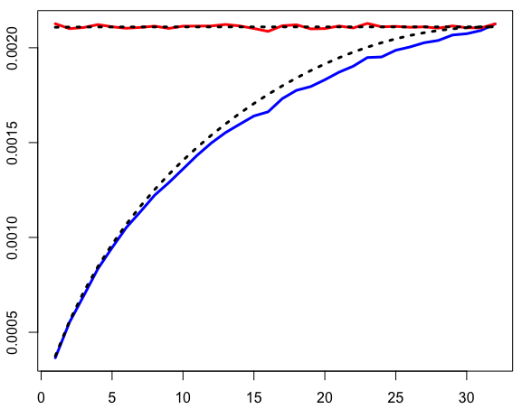
a) Frobenius risks for ,
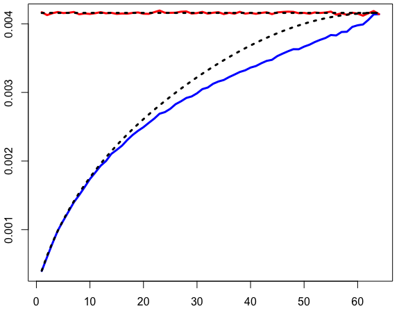
b) Frobenius risks for ,
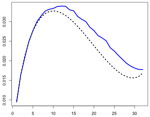
c) Bures risks for ,
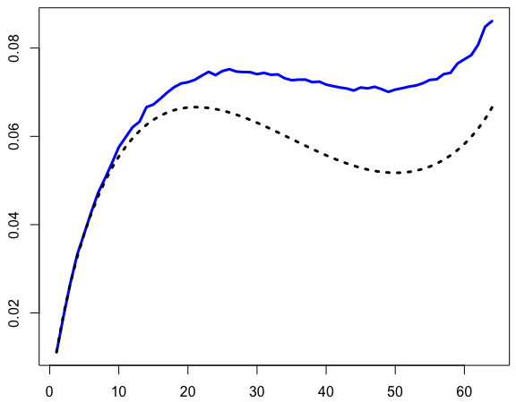
d) Bures risks for ,
9 Comparative numerical simulations
In this section we detail the methodology and results of a general simulation study which compares the performance of the estimators presented in the previous sections for a set of states and against several estimation criteria. The states we consider are rank- states with a fixed spectrum of equal eigenvalues of magnitude each, and have randomly generated eigenvectors. This choice is motivated by the fact that such states are arguably harder to estimate among rank-r states (in analogy to the fact that an unbiased coin is harder to estimate than a biased one. Additionally, having such a spectrum allows for a more consistent comparison of the estimators across several ranks.
We generate the above mentioned states for or qubits, and for a particular ‘true state’ we simulate a dataset of counts from which the state is to be reconstructed. The outcome statistics depend on a few variables that we may vary, namely the type of measurement design (random basis vs Pauli), the number of repetitions per settings , and in the case of the random basis measurements the total number of measured settings. This allows us to study the performance of the estimators across several different combinations of variables: types of states, ranks, measurement design, number of repetitions per setting , the total number of settings and the number of ions .
We will present plots of the estimated mean errors of the estimators for the equal eigenvalues states. For each given rank and number of qubits , we generate a state with equal eigenvalues and random eigenbasis. Then for each choice of measurement design and values of and , the several estimates of the true state are evaluated. The error of each resulting estimate is computed using all the error functions listed in Table 1, and the corresponding mean errors are estimated from 100 different runs of the experiment.
In order to make the results of the simulation study more accessible, we have made all plots for 3 and 4 atoms simulation available online via an interactive Rshiny application at this address: https://rudhacharya.shinyapps.io/plots/, while a selection is presented in the paper.
9.1 Squared Frobenius norm
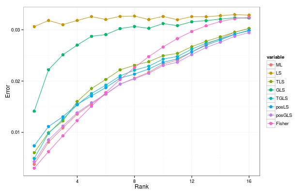
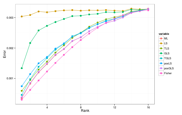
Figures 4 and 5 show the (estimated) Frobenius risk (mean square error) for states 4 qubits measured with the Pauli and the random basis design, respectively. The states are chosen randomly from the family of rank- states with equal non-zero eigenvalues. In both cases we note that the Frobenius risk of the LS estimator has no significant dependence on the rank of the true state, and its performance is poor for small rank states. In contrast, the remaining estimators all show a scaling of the Frobenius risk with the rank of the true state. We also note that the performance of several of the estimators matches well with the Fisher-predicted risk. This is remarkable as the latter (6) was defined for a rank- parameterisation of states, while none of the estimators have any prior knowledge of the rank.
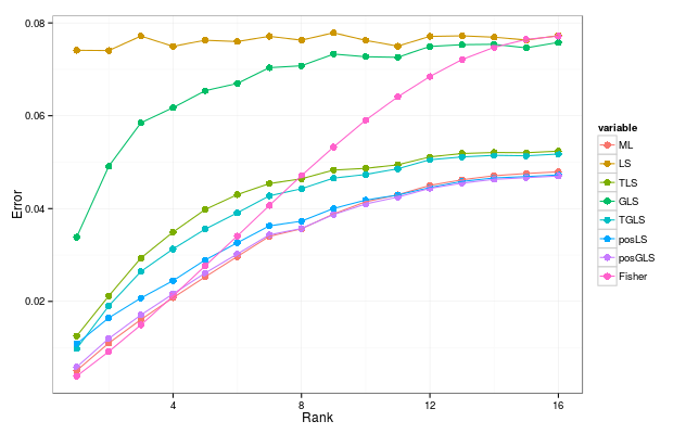
a) , and
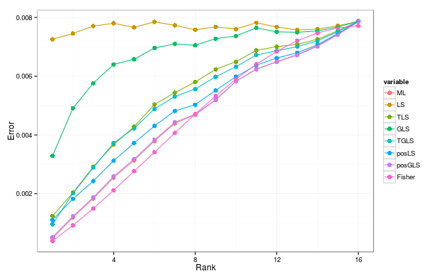
b) , and
a) , and
b) , and
We further note that for relatively small values of the TLS, TGLS, posLS, posGLS, ML estimators significantly better that LS and GLS at higher ranks, while the errors approach each other for larger , cf. Figures 4 a) and 5 a) versus 4 b) and 5 b). This reflects the fact that in the low case the asymptotic regime has not been reached and constrained estimators have an advantage even for full rank states which lie in the interior of the parameter space. Indeed for an eigenvalue of order and relatively small values of , the unconstrained estimates will have a standard deviation of order which may be comparable or larger than the magnitude of the eigenvalues themselves. Therefore without the constraint of positivity such estimators may produce estimates with . In contrast, for the constrained estimators the positivity constraint provides additional information when the eigenvalues are small. For large values of however, the uncertainty in the eigenvalues is very small and the Fisher risk acts as a lower bound for all of the estimators.
Across both the Pauli and the random measurement designs we note that the performance of the posGLS and the ML estimators is very similar, and for large almost identical. This confirms our asymptotic analysis which shows that the posGLS and the ML estimators are equivalent in the limit of large , cf. section 7.2.
9.2 Bures and Hellinger distance
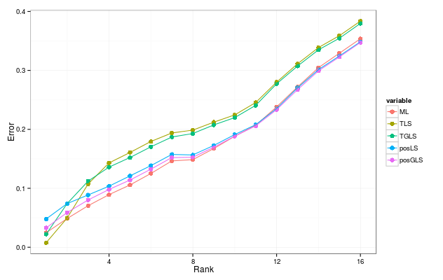
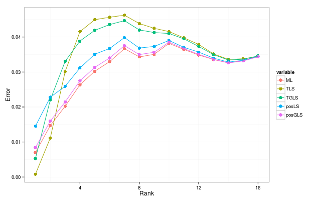
As the Bures distance is well defined only over density matrices, we plot the mean Bures errors only for the ML, TLS, TGLS, posLS , posGLS estimators. Figures 6 and 7 show the mean Bures errors for different sample sizes in the Pauli, and respectively random bases measurement design. For comparison, in Figures 8 and 9 we also plot the corresponding average Hellinger errors , cf. Table 1.
We note that the behaviour of the Hellinger errors is very similar to that of the Bures errors, with a better match for larger values of . To give some intuition about this, we look at what happens in the case of qubits. The Bures distance between neighbouring qubit states can be approximated by the sum of Hellinger distance and a quadratic form in the parameters of the unitary connecting the eigenbases of the two states [4]
| (39) |
where is the angle between the Bloch vectors of and . In a non-adaptive measurement scenario such as those considered here, the Bloch vector parameters can be estimated at rate which means that the second term on the right side of (39) is always of the order . However, for states which are very pure () the Hellinger component has the dominant contribution to the Bures distance, and is responsible for the “non-standard” scaling of in the minimax risk [4]. The simulation results indicate that a similar phenomenon may occur in higher dimensional systems. For full rank states, both the Bures and the Hellinger distance have a quadratic expansion, and in this sense a relation similar to (39) can be derived by splitting the Bures distance into quadratic contributions coming from changes in the eigenvalues and small basis rotations respectively, see also [61]. Alternatively, the block-matrix techniques used for analysing the Bures risk in section 8.1 can be extended to rank deficient states of arbitrary spectrum to show that the leading contribution comes from the Hellinger
Another noticeable feature across both the Pauli and the random bases measurement design is that for large the mean errors are seen to be larger for states of middling ranks than for the full rank states, see Figures 6b, 7b. This is however not true for smaller values of , as shown in Figures 6a, 7a. More precisely, for large we see a steep increase from pure states to low rank states, followed by an almost linear decrease down to the full rank state. A similar behaviour has been uncovered in the analysis of the PLS estimator for covariant measurements in section 8.1. There, we found that for large and low rank , the eigenvalues distribution of the error block of the LS estimator converges to the Wigner distribution, which allows us to compute the leading orders of the Bures risk of the PLS estimator. Since the covariant measurement arises in the large limit of the random basis measurement [3], it is therefore expected that the risks behave similarly in the two cases. Our simulations indicate that the mechanism governing the asymptotics of the Bures risk seems to be robust with respect to the details of the measurement; although the Pauli basis measurement is not expected to produce an LS estimator whose error matrix is Wigner distributed, the Bures and Hellinger risks have similar characteristics as those of the covariant measurement. These findings are in line with those of [66], and are worthy of further theoretical investigation.
a) , and
b) , and
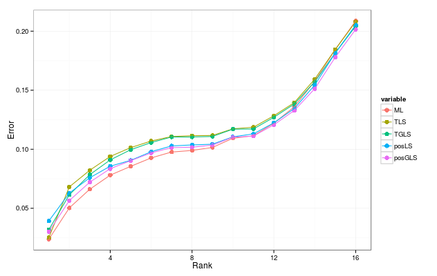
a) , and
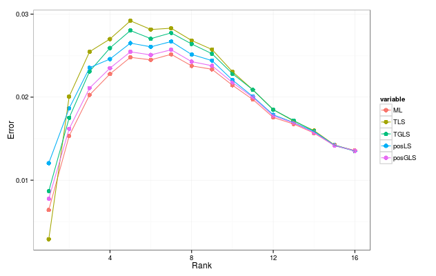
b) , and
While the Bures risk for rank deficient states scales as , for full rank states the Bures distance is locally quadratic, and standard asymptotic results imply that the convergence rate is in this case , cf. section 3.1. In general,
with weight matrix , where is the quantum Fisher information. For the maximally mixed state , and the parametrisation (4), the latter has 2 uncorrelated blocks [3] corresponding to off-diagonal parameters
and respectively diagonal parameters
On the other hand, the classical average Fisher information for random basis measurements is given by [17]. Since the ML estimator is asymptotically normal with variance , we have
For 3 qubits with samples, and 4 qubits with , the asymptotic predictions for Bures errors are and which match closely the simulations results [1].
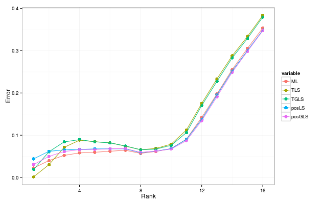
a) , and
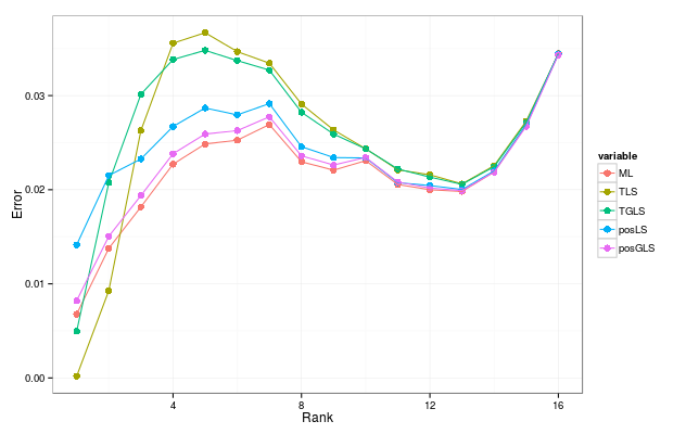
b) , and
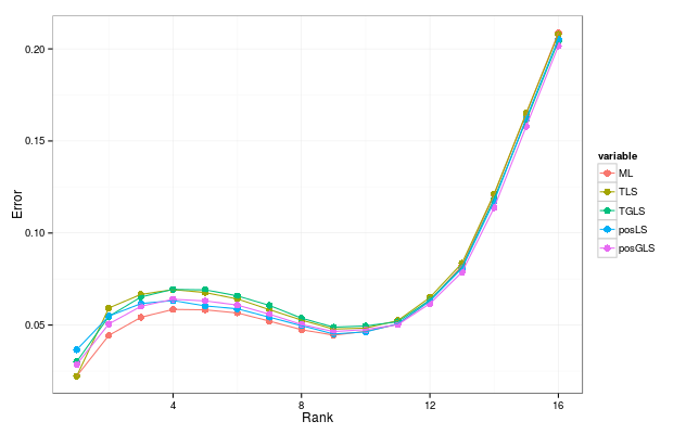
a) , and
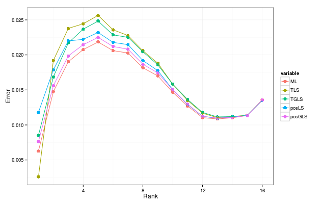
b) , and
9.3 Trace-norm distance
The risks for the trace-norm distance exhibit a similar behaviour to those of the Frobenius distance, as illustrated in Figures 10 and 11. A noticeable feature is that all constrained estimators have close risks for large sample sizes in both the Pauli and the random bases setting.
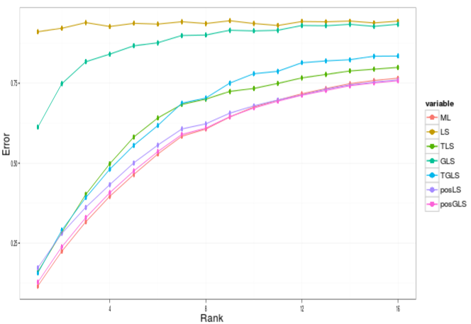
a) ,
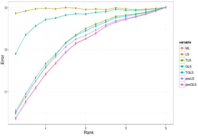
b) ,
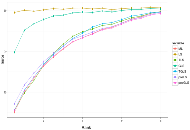
a) , and
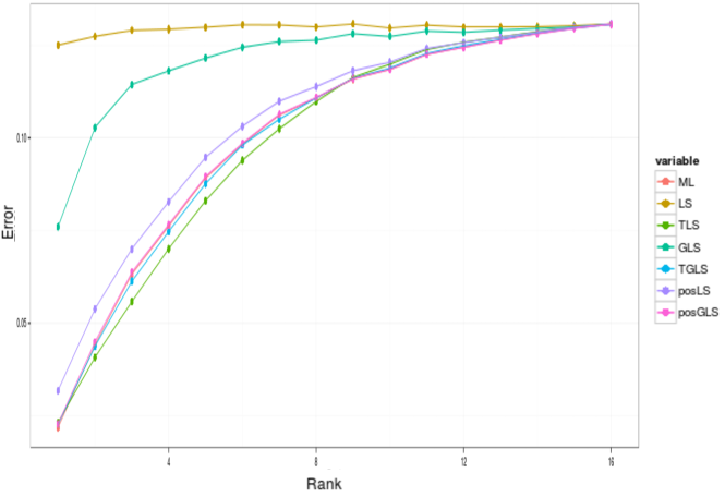
b) , and
10 Conclusions
In this paper we studied theoretical an practical aspects of quantum tomography methods. The unifying theme is that each estimator can be seen as a projection of the data onto a parameter space with respect to an appropriate metric. We considered estimators without positivity constraints (unconstrained maximum likelihood, least squares, generalised least squares) and with positivity constraints (maximum likelihood, positive least squares, thresholded least squares and projected least squares), and investigated the relationships between different estimators. While no estimator makes use of the state’s rank (which is assumed to be unknown) the constrained estimators have significantly lower errors than the unconstrained estimators, for low rank states. To better understand this behaviour we derived new asymptotic error rates for the least squares estimator and for the projected least squares estimators, for a class of given rank states and covariant measurements. These results capture the exact rate dependence on rank and dimension and complement non-asymptotic concentration bounds of [17, 72, 36], showing that PLS has strong optimality properties; for instance the leading contribution to the Frobenius risk is which is ‘almost optimal’, in that it is only 3 times larger than the minimax lower bound established in [17], which assumes that the rank is known. Our analysis has uncovered an interesting behaviour of the Bures error, which increases with respect to rank for small ranks and then decreases towards full rank states. The extensive simulations study shows that this behaviour (as well as the monotonic increase of other errors) is robust with respect to the measurement design.
Computationally, maximum likelihood and positive least squares involve an optimisation over states and are significantly slower than projected least squares which only requires the diagonalisation of the least squares matrix followed by a simple truncation procedure. Our results confirm and strengthen those of [36] and show that projected least squares is an attractive alternative to maximum likelihood, which is routinely used in practice. Additional improvements can be achieved by using generalised least squares as starting point, in a two steps procedure.
An interesting and practically relevant open question is whether any of the ‘fast’ estimators analysed here is statistically ‘optimal’ for more realistic measurements such as the Pauli bases. More generally, one can ask whether these methods can be adapted to non-informationally complete measurement scenarios, and other physically motivated lower dimensional statistical models.
Acknowledgements. We thank Jonas Kahn, Richard Kueng and Ian Dryden for fruitful discussions during the preparation of this manuscript.
Appendix A Appendix
A.1 Fisher information for GLS
Here we prove the equality stated in section 5.1. Note that by definition
and
| (40) |
We will show that
| (41) |
where are some constants and is the vector whose entries are the inverses of measurement probabilities. Indeed, since , equation (41) implies (40).
Now is the pseudo-inverse of and since , it satisfies
To compute the inverse on the right side we use the definition (17) of and apply the Sherman-Morrison formula [68]
This gives
| (42) |
where . By applying the Sherman-Morrison formula again we get
where . Moreover,
By plugging the last three expresssions into (42) we get
which concludes the proof of (41) and of .
A.2 Implementations of estimators
Here we list certain practical details about the implementation of the estimators described in the paper. In particular we discuss how we compute the covariance matrix estimator used in the GLS, TGLS, posGLS estimators, and we also describe the cross-validation procedure we use to select a constant for the thresholded in the TLS and TGLS estimators.
-
1.
The covariance matrix estimator for the generalised estimators (GLS, TGLS and posGLS) is computed as follows. Given a dataset , we first obtain the LS estimate and then construct the TLS estimate (see Algorithm 1) with threshold . From this we obtain an estimate of the probabilities . The matrix is then constructed from these estimated probabilities via (17). The generalised estimates (GLS/TGLS/posGLS) are then evaluated using and the same dataset .
-
2.
As mentioned briefly in section 6, the threshold for the TLS and TGLS estimators is selected using cross-validation. We describe this cross-validation method below [17].
-
•
For a particular number of repetitions per setting , we simulate data in 5 independent batches repetitions per setting in each batch. and we denote the corresponding datasets as . The total dataset of counts is the sum .
-
•
We choose a vector of constants forming a mesh over the interval . For each value of , and for each we compute the following estimators. We hold out the dataset , and compute the TLS/TGLS estimate for the dataset , with threshold , cf. [17]. For each the LS estimate is also evaluated.
-
•
For all values of , the empirical discrepancy is evaluated for a choice of error function
-
•
This function is then minimised over all values
this gives an estimate for the holding constant, which is then used to evaluate the TLS or the TGLS estimators with threshold .
Notice that the cross-validation procedure picks different constants for different choices of the error function. An important caveat here is that the Bures distance is not defined for the LS estimates , and therefore the procedure above cannot apply. Instead in the simulations we estimate the thresholding constant using the ML estimate as
-
•
References
- [1] Complete simulation results. https://rudhacharya.shinyapps.io/plots/.
- [2] Cvx: Matlab software for disciplined convex programming. http://cvxr.com/cvx/, 2017.
- [3] A. Acharya and M. Guta. Statistical analysis of compressive low rank tomography with random measurements. Journal of Physics A: Mathematical and Theoretical, 50(19):195301, 2017.
- [4] A. Acharya and M. Guta. Minimax estimation of qubit states with Bures risk. Journal of Physics A: Mathematical and Theoretical, 51:175307, 2018.
- [5] A. Acharya, T. Kypraios, and M. Guta. Statistically efficient tomography of low rank states with incomplete measurements. New Journal of Physics, 18(4):043018, 2016.
- [6] L. Artiles, R. D. Gill, and M. Guta. An invitation to quantum tomography. J. Royal Statist. Soc. B (Methodological), 67:109–134, 2005.
- [7] Koenraad M R Audenaert and Stefan Scheel. Quantum tomographic reconstruction with error bars: a kalman filter approach. New Journal of Physics, 11(2):023028, 2009.
- [8] E. Bagan, M. Baig, and R. Munoz-Tapia. Optimal scheme for estimating a pure qubit state via local measurements. Phys. Rev. Lett., 89:277904, 2002.
- [9] E. Bagan, M. A. Ballester, R. D. Gill, A. Monras, and R. Munoz-Tapia. Optimal full estimation of qubit mixed states. Phys. Rev. A, 73:032301, 2006.
- [10] K. Banaszek, G. M. D’Ariano, M. G. A. Paris, and M. F. Sacchi. Maximum-likelihood estimation of the density matrix. Physical Review A, 61, 1999.
- [11] O. E. Barndorff-Nielsen, Gill, R. D., and Jupp, P. E. On quantum statistical inference (with discussion). J. R. Statist. Soc. B, 65:775–816, 2003.
- [12] T. Baumgratz, A. Nüßeler, M. Cramer, and M. B. Plenio. A scalable maximum likelihood method for quantum state tomography. New Journal of Physics, 15(12):125004, 2013.
- [13] V. P. Belavkin. Generalized uncertainty relations and efficient measurements in quantum systems. Theoretical and Mathematical Physics, 26:213–222, 1976.
- [14] R. Blume-Kohout. Hedged maximum likelihood quantum state estimation. Phys. Rev. Lett., 105:200504, 2010.
- [15] R. Blume-Kohout. Optimal, reliable estimation of quantum states. New Journal of Physics, 12(4):043034, 2010.
- [16] S. L. Braunstein and C. M. Caves. Statistical distance and the geometry of quantum states. Phys. Rev. Lett., 72:3439–3443, May 1994.
- [17] C. Butucea, M. Guta, and T. Kypraios. Spectral thresholding quantum tomography for low rank states. New Journal of Physics, 17(11):113050, 2015.
- [18] M. Christandl and R. Renner. Reliable quantum state tomography. Phys. Rev. Lett., 109:120403, Sep 2012.
- [19] B. Collins and P. Śniady. Integration with respect to the haar measure on unitary, orthogonal and symplectic group. Communications in Mathematical Physics, 264:773–795, 2006.
- [20] M. Cramer, M. B. Plenio, S. T. Flammia, R. Somma, D. Gross, S. D. Bartlett, O. Landon-Cardinal, D. Poulin, and Y.-K. Liu. Efficient quantum state tomography. Nat Commun, 1:149, 12 2010.
- [21] G. M. D’Ariano, Macchiavello, C., and Paris, M. G. A. Detection of the density matrix through optical homodyne tomography without filtered back projection. Phys. Rev. A, 50:4298–4302, 1994.
- [22] I. L. Dryden, Le. H., S. P. Preston, and A. T. A. Wood. Mean shapes, projections and intrinsic limiting distributions. Journal of Statistical Planning and Inference, 145:25–32, 2014.
- [23] Laszlo Erdös. Universality of wigner random matrices: a survey of recent results. Russian Mathematical Surveys, 66(3):507, 2011.
- [24] P. Faist and R. Renner. Practical and reliable error bars in quantum tomography. Phys. Rev. Lett., 117:010404, Jul 2016.
- [25] C. Ferrie and R. Blume-Kohout. Minimax quantum tomography: Estimators and relative entropy bounds. Phys. Rev. Lett., 116:090407, 2016.
- [26] Christopher Ferrie. Self-guided quantum tomography. Phys. Rev. Lett., 113:190404, Nov 2014.
- [27] S. T. Flammia, D. Gross, Y.-K. Liu, and J. Eisert. Quantum tomography via compressed sensing: error bounds, sample complexity and efficient estimators. New Journal of Physics, 14:095022, 2012.
- [28] A. Fujiwara and H. Nagaoka. Quantum fisher metric and estimation for pure state models. Phys. Lett A, 201:119–124, 1995.
- [29] W.-B. Gao, C.-Y. Lu, X.-C. Yao, P. Xu, O. Guhne, A. Goebel, Y.-A. Chen, C.-Z. Peng, Z.-B. Chen, and J.-W. Pan. Experimental demonstration of a hyper-entangled ten-qubit schrodinger cat state. Nat Phys, pages 331–335, 2010.
- [30] R. D. Gill and M. Guta. On asymptotic quantum statistical inference. From Probability to Statistics and Back: High-Dimensional Models and Processes, 9(10.1214/12-IMSCOLL909):105–127, 2013.
- [31] R. D. Gill and S. Massar. State estimation for large ensembles. Phys. Rev. A, 61:042312, 2000.
- [32] D. S. Goncalves, M. A. Gomes-Ruggiero, C. Lavor, O. J. Farias, and P. H. S. Ribeiro. Local solutions of maximum likelihood estimation in quantum state tomography. arXiv:1103.3682v2, 2012.
- [33] C. Granade, J. Combes, and D. G. Corrie. Practical bayesian tomography. new Journal of Physics, 18:033024, 2016.
- [34] C. Granade, C. Ferrie, and S. T. Flammia. Practical adaptive quantum tomography. New Journal of Physics, 19(11):113017, 2017.
- [35] D. Gross, Y.-K. Liu, S. T. Flammia, S. Becker, and J. Eisert. Quantum state tomography via compressed sensing. Phys. Rev. Lett., 105:150401, 2010.
- [36] M. Guta, J. Kahn, R. Kueng, and J. A. Tropp. Fast state tomography with optimal error bounds. arXiv:1809.11162, 2018.
- [37] J Haah, A. W. Harrow, Z. Ji, X. Wu, and N. Yu. Sample-optimal tomography of quantum states. IEEE Transactions on Information Theory, 63:5628–5641, 2017.
- [38] H. Haffner, W. Hansel, C. F. Roos, J. Benhelm, D. Chek-al kar, M. Chwalla, T. Korber, U. D. Rapol, M. Riebe, P. O. Schmidt, C. Becher, O. Guhne, W. Dur, and R. Blatt. Scalable multiparticle entanglement of trapped ions. Nature, pages 643–646, 2005.
- [39] Th. Hannemann, D. Reiss, Ch. Balzer, W. Neuhauser, P. E. Toschek, and Ch. Wunderlich. Self-learning estimation of quantum states. Phys. Rev. A, 65:050303, May 2002.
- [40] M. Hayashi, editor. Asymptotic theory of quantum statistical inference: selected papers. World Scientific, 2005.
- [41] M. Hayashi and K. Matsumoto. Asymptotic performance of optimal state estimation in qubit system. J. Math. Phys., 49:102101–33, 2008.
- [42] C. W. Helstrom. Quantum detection and estimation theory. Journal of Statistical Physics, 1:231–252, 1969.
- [43] A. S. Holevo. Probabilistic and Statistical Aspects of Quantum Theory, volume 1. Edizioni della Normale, 1 edition, 2011.
- [44] D. F. V. James, P. G. Kwiat, W. J. Munro, and A. G. White. Measurement of qubits. Phys. Rev. A, 64:052312, 2001.
- [45] J. Kahn and M. Guta. Local asymptotic normality for finite dimensional quantum systems. Communications in Mathematical Physics, 289(2):597–652, Jul 2009.
- [46] A. Kalev and C. H. Baldwin. The power of being positive: Robust state estimation made possible by quantum mechanics. arXiv preprint arXiv:1511.01433, November 2015.
- [47] M. Keyl and R. F. Werner. Estimating the spectrum of a density operator. Phys. Rev. A, 64:052311, 2001.
- [48] V. Koltchinskii and D. Xia. Optimal estimation of low rank density matrices. Journal of Machine Learning Research, 16:1757–1792, 2015.
- [49] R. Kueng, H. Rauhut, and U. Terstiege. Low rank matrix recovery from rank one measurements. Appl. Comput. Harmon. Anal., 42(1):88 – 116, 2017.
- [50] B. P. Lanyon, C. Maier, M. Holzäpfel, T. Baumgratz, C. Hempel, P. Jurcevic, I. Dhand, A. S. Buyskikh, A. J. Daley, M. Cramer, M. B. Plenio, R. Blatt, and C. F. Roos. Efficient tomography of a quantum many-body system. Nature Physics, 13:1158–1162, 2017.
- [51] E. L. Lehmann and G. Casella. Theory of point estimation. Springer, 1998.
- [52] U. Leonhardt. Essential Quantum Optics From Quantum Measurements to Black Holes. Number 9780521869782. Cambridge University Press, 1 edition, March 2010.
- [53] X. Li, J. Shang, H. K. Ng, and B.-G. Englert. Optimal error intervals for properties of the quantum state. Phys. Rev. A, 94:062112, Dec 2016.
- [54] Y.-K. Liu. Universal low-rank matrix recovery from pauli measurements. In Advances in Neural Information Processing Systems 24: 25th Annual Conference on Neural Information Processing Systems 2011. Proceedings of a meeting held 12-14 December 2011, Granada, Spain., pages 1638–1646, 2011.
- [55] D. H. Mahler, L. A. Rozema, A. Darabi, C. Ferrie, R. Blume-Kohout, and A. M. Steinberg. Adaptive quantum state tomography improves accuracy quadratically. Phys. Rev. Lett., 111:183601, Oct 2013.
- [56] S. Massar and S Popescu. Optimal extraction of information from finite quantum ensembles. Phys. Rev. Lett., 74:1259–1263, 1995.
- [57] K. Matsumoto. A new approach to the cramer-rao type bound of the pure state model. J. Phys. A, 35(13):3111–3123, 2002.
- [58] T. Monz, P. Schindler, J. T. Barreiro, M. Chwalla, D. Nigg, W. A. Coish, M. Harlander, W. Hänsel, M. Hennrich, and R. Blatt. 14-qubit entanglement: Creation and coherence. Phys. Rev. Lett., 106:130506, 2011.
- [59] M. G. A. Paris and J. Rehacek, editors. Quantum state estimation. Number 649 in Lecture Notes in Physics. Springer, Berlin Heidelberg, 2004.
- [60] L. Pereira, L. Zambrano, J. Cortés-Vega, S. Niklitschek, and A. Delgado. Adaptive quantum tomography in high dimensions. Phys. Rev. A, 98:012339, 2018.
- [61] L. Pereira, L. Zambrano, J. Cortés-Vega, S. Niklitschek, and A. Delgado. Adaptive quantum tomography in high dimensions. Phys. Rev. A, 98:012339, 2018.
- [62] D. Petz and Jencova, A. Sufficiency in quantum statistical inference. Commun. Math. Phys., 263:259 – 276, 2006.
- [63] B. Qi, Z. Hou, L. Li, D. Dong, G. Xiang, and G. Guo. Quantum state tomography via linear regression estimation. Scientific Reports, 3:3496 EP –, 2013.
- [64] J. Rehacek, Z. Hradil, E. Knill, and A. I. Lvovsky. Diluted maximum-likelihood algorithm for quantum tomography. Phys. Rev. A, 75:042108, 2007.
- [65] J. H. Schenker and H. Schulz-Baldes. Semicircle law and freeness for random matrices with symmetries or correlations. Mathematical Research Letters, 12:531–542, 2005.
- [66] T. L. Scholten and R. Blume-Kohout. Behavior of the maximum likelihood in quantum state tomography. New Journal of Physics, 023050:20, 2018.
- [67] C. Schwemmer, G. Tóth, A. Niggebaum, T. Moroder, D Gross, O. Gühne, and H. Weinfurter. Experimental comparison of efficient tomography schemes for a six-qubit state. Phys. Rev. Lett., 113:040503, Jul 2014.
- [68] J. Sherman and W. J. Morrison. Adjustment of an inverse matrix corresponding to a change in one element of a given matrix. Ann. Math. Statist., 21:124–127, 1950.
- [69] John A. Smolin, Jay M. Gambetta, and Graeme Smith. Efficient method for computing the maximum-likelihood quantum state from measurements with additive gaussian noise. Phys. Rev. Lett., 108:070502, Feb 2012.
- [70] A. Steffens, C. A. Riofrío, W. McCutcheon, I Roth, B. A. Bell, A. McMillan, M. S. Tame, J. G. Rarity, and J. Eisert. Experimentally exploring compressed sensing quantum tomography. Quantum Science and Technology, 2(2):025005, 2017.
- [71] D. Suess, L. Rudnicki, T. O. Maciel, and D. Gross. Error regions in quantum state tomography: computational complexity caused by geometry of quantum states. New Journal of Physics, 19(9):093013, 2017.
- [72] T. Sugiyama, P. S. Turner, and M. Murao. Precision-guaranteed quantum tomography. Phys. Rev. Lett., 111:160406, 2013.
- [73] Moroder. T., P. Hyllus, G. Tóth, C. Schwemmer, A. Niggebaum, S. Gaile, O. Gühne, and H. Weinfurter. Permutationally invariant state reconstruction. New Journal of Physics, 14(10):105001, 2012.
- [74] Yong Siah Teo, Berthold-Georg Englert, Jaroslav Řeháček, Zdeněk Hradil, and Dmitry Mogilevtsev. Verification of state and entanglement with incomplete tomography. New Journal of Physics, 14:105020, 2012.
- [75] Yong Siah Teo, Huangjun Zhu, Berthold-Georg Englert, Jaroslav Řeháček, and Zden ěk Hradil. Quantum-state reconstruction by maximizing likelihood and entropy. Phys. Rev. Lett., 107:020404, 2011.
- [76] J. A. Tropp. User-friendly tail bounds for sums of random matrices. Found. Comput. Math., 12(4):389–434, 2012.
- [77] G. Vidal, J. I. Latorre, P. Pascual, and R. Tarrach. Optimal minimal measurements of mixed states. Phys. Rev. A, 60:126, 1999.
- [78] G. A. Young and R. L. Smith. Essentials of statistical inference. Cambridge University Press, 2005.
- [79] H. P. Yuen and M. Lax. Multiple-parameter quantum estimation and measurement of non-selfadjoint observables. IEEE Trans. Inform. Theory, 19:740, 1973.