Resource-aware IoT Control: Saving Communication through Predictive Triggering
Abstract
The Internet of Things (IoT) interconnects multiple physical devices in large-scale networks. When the ‘things’ coordinate decisions and act collectively on shared information, feedback is introduced between them. Multiple feedback loops are thus closed over a shared, general-purpose network. Traditional feedback control is unsuitable for design of IoT control because it relies on high-rate periodic communication and is ignorant of the shared network resource. Therefore, recent event-based estimation methods are applied herein for resource-aware IoT control allowing agents to decide online whether communication with other agents is needed, or not. While this can reduce network traffic significantly, a severe limitation of typical event-based approaches is the need for instantaneous triggering decisions that leave no time to reallocate freed resources (e.g., communication slots), which hence remain unused. To address this problem, novel predictive and self triggering protocols are proposed herein. From a unified Bayesian decision framework, two schemes are developed: self triggers that predict, at the current triggering instant, the next one; and predictive triggers that check at every time step, whether communication will be needed at a given prediction horizon. The suitability of these triggers for feedback control is demonstrated in hardware experiments on a cart-pole, and scalability is discussed with a multi-vehicle simulation.
Index Terms:
Internet of Things, feedback control, event-based state estimation, predictive triggering, self triggering, distributed control, resource-aware control.I Introduction
The Internet of Things (IoT) will connect large numbers of physical devices via local and global networks, [1, 2]. While early IoT research concentrated on problems of data collection, communication, and analysis [3], using the available data for actuation is vital for envisioned applications such as autonomous vehicles, building automation, or cooperative robotics. In these applications, the devices or ‘things’ are required to act intelligently based on data from local sensors and the network. For example, cars in a platoon need to react to other cars’ maneuvers to keep a desired distance; and climate control units must coordinate their action for optimal ambience in a large building. IoT control thus refers to systems where data about the physical processes, collected via sensors and communicated over networks, are used to decide on actions. These actions in turn affect the physical processes, which is the core principle of closed-loop control or feedback.
Figure 1 shows an abstraction of a general IoT control system. When the available information within the IoT is used for decision making and commanding actuators (red arrows), one introduces feedback between the cyber and the physical world, [3]. Feedback loops can be closed on the level of a local object, but, more interestingly, also across agents and networks. Coordination among agents is vital, for example, when agents seek to achieve a global objective. IoT control aims at enabling coordinated action among multiple things.
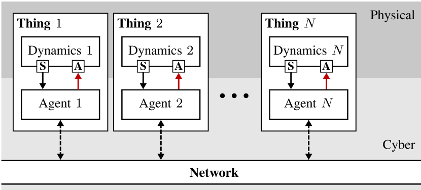
In contrast to traditional feedback control systems, where feedback loops are closed over dedicated communication lines (typically wires), feedback loops in IoT control are realized over a general purpose network such as the Internet or local networks. In typical IoT applications, these networks are wireless. While networked communication offers great advantages in terms of, inter alia, reduced installation costs, unprecedented flexibility, and availability of data, control over networks involves formidable challenges for system design and operation, for example, because of imperfect communication, variable network structure, and limited communication resources, [4, 5]. Because the network bandwidth is shared by multiple entities, each agent should use the communication resource only when necessary. Developing such resource-aware control for the IoT is the focus of this work. This is in contrast to traditional feedback control, where data transmission typically happens periodically at a priori fixed update rates.
Owing to the shortcomings of traditional control, event-based methods for state estimation and control have emerged since the pioneering work [6, 7]. The key idea of event-based approaches is to apply feedback only upon certain events indicating that transmission of new data is necessary (e.g., a control error passing a threshold level, or estimation uncertainty growing too large). Core research questions concerning the design of the event triggering laws, which decide when to transmit data, and the associated estimation and control algorithms with stability and performance guarantees have been solved in recent years (see [8, 9, 10, 11] for overviews).
This work builds on a framework for distributed event-based state estimation (DEBSE) developed in prior work [12, 13, 14, 15], which is applied herein to resource-aware IoT control as in Fig. 1. The key idea of DEBSE is to employ model-based predictions of other things to avoid the need for continuous data transmission between the agents. Only when the model-based predictions become too inaccurate (e.g., due to a disturbance or accumulated error), an update is sent. Figure 2 represents one agent of the IoT control system in Fig. 1 and depicts the key components of the DEBSE architecture:
-
•
Local control: Each agent makes local control decisions for its actuator; for coordinated action across the IoT, it also needs information from other agents in addition to its local sensors.
-
•
Prediction of other agents: State estimators and predictors (e.g., of Kalman filter type) are used to predict the states of all, or a subset of agents based on agents’ dynamics models; these predictions are reset (or updated) when new data is received from the other agents.
-
•
Event trigger: Decides when an update is sent to all agents in the IoT. For this purpose, the local agent implements a copy of the predictor of its own behavior (Prediction Thing ) to replicate locally the information the other agents have about itself. The event trigger compares the prediction with the local state estimate: the current state estimate is transmitted to other agents only if the prediction is not sufficiently accurate.
Key benefits of this architecture are: each agent has all relevant information available for coordinated decision making, but inter-agent communication is limited to the necessary instants (whenever model-based predictions are not good enough).

Experimental studies [12, 14] demonstrated that DEBSE can achieve significant communication savings, which is inline with many other studies in event-based estimation and control. The research community has had remarkable success in showing that the number of samples in feedback loops can be reduced significantly as compared to traditional time-triggered designs. This can be translated into increased battery life [16] in wireless sensor systems, for example. Despite these successes, better utilization of shared communication resources has typically not been demonstrated. A fundamental problem of most event-triggered designs (incl. DEBSE) is that they make decisions about whether a communication is needed instantaneously. This means that the resource must be held available at all times in case of a positive triggering decision. Conversely, if a triggering decision is negative, the reserved slot remains unused because it cannot be reallocated to other users immediately.
In order to translate the reduction in average sampling rates to better actual resource utilization, it is vital that the event-based system is able to predict resource usage ahead of time, rather than requesting resources instantaneously. This allows the processing or communication system to reconfigure and make unneeded resources available to other users or set to sleep for saving energy. Developing such predictive triggering laws for DEBSE and their use for resource-aware IoT control are the main objectives of this article.
Contributions
This article proposes a framework for resource-aware IoT control based on DEBSE. The main contributions are summarized as follows:
-
1.
Proposal of a Bayesian decision framework for deriving predictive triggering mechanisms, which provides a new perspective on the triggering problem in estimation;
-
2.
Derivation of two novel triggers from this framework: the self trigger, which predicts the next triggering instant based on information available at a current triggering instant; and the predictive trigger, which predicts triggering for a given future horizon of steps;
-
3.
Demonstration and comparison of the proposed triggers in experiments on an inverted pendulum testbed; and
-
4.
Simulation study of a multi-vehicle system.
The Bayesian decision framework extends previous work [17] on event trigger design to the novel concept of predicting trigger instants. The proposed self trigger is related to the concept of variance-based triggering [13], albeit this concept has not been used for self triggering before. To the best of the authors’ knowledge, predictive triggering is a completely new concept in both event-based estimation and control. Predictive triggering is shown to reside between the known concepts of event triggering and self triggering.
A preliminary version of some results herein was previously published in the conference paper [18]. This article targets IoT control and has been restructured and extended accordingly. New results beyond [18] include the treatment of control inputs in the theoretical analysis (Sec. V), the discussion of multiple agents (Sec. VIII), hardware experiments (Sec. VII), and a new multi-vehicle application example (Sec. IX).
II Related Work
Because of the promise to achieve high-performance control on resource-limited systems, the area of event-based control and estimation has seen substantial growth in the last decades. For general overviews, see [8, 9, 4, 10] for control and [8, 17, 19, 11] for state estimation. This work mainly falls in the category of event-based state estimation (albeit state predictions and estimates are also used for feedback, cf. Fig. 2).
Various design methods have been proposed in literature for event-based state estimation and, in particular, its core components, the prediction/estimation algorithms and event triggers. For the former, different types of Kalman filters [12, 13, 20], modified Luenberger-type observers [14, 15], and set-membership filters [21, 22] have been used, for example. Variants of event triggers include triggering based on the innovation [12, 23], estimation variance [13, 24], or entire probability density functions (PDFs) [25]. Most of these event triggers make transmit decisions instantaneously, while the focus of this work is on predicting triggers.
The concept of self triggering has been proposed [26] to address the problem of predicting future sampling instants. In contrast to event triggering, which requires the continuous monitoring of a triggering signal, self-triggered approaches predict the next triggering instant already at the previous trigger. While several approaches to self-triggered control have been proposed in literature (e.g., [9, 27, 28, 29]), self triggering for state estimation has received considerably less attention. Some exceptions are discussed next.
Self triggering is considered for set-valued state estimation in [30], and for high-gain continuous-discrete observers in [31]. In [30], a new measurement is triggered when the uncertainty set about some part of the state vector becomes too large. In [31], the triggering rule is designed so as to ensure convergence of the observer. The recent works [32] and [33] propose self triggering approaches, where transmission schedules for multiple sensors are optimized at a-priori fixed periodic time instants. While the re-computation of the schedule happens periodically, the transmission of sensor data does generally not. In [34], a discrete-time observer is used as a component of a self-triggered output feedback control system. Therein, triggering instants are determined by the controller to ensure closed-loop stability.
Alternatives to the Bayesian decision framework herein for developing triggering schedules include dynamic programming approaches such as in [35, 36, 37].
None of the mentioned references considers the approach taken herein, where triggering is formulated as a Bayesian decision problem under different information patterns. The concept of predictive triggering, which is derived from this, is novel. It is different from self triggering in that decisions are made continuously, but for a fixed prediction horizon.
III Fundamental Triggering Problem
In this section, we formulate the predictive triggering problem that each agent in Fig. 2 has to solve, namely predicting when local state estimates shall be transmitted to other agents of the IoT. We consider the setup in Fig. 3, which has been reduced to the core components required for the analysis in subsequent sections. Agent , called sensor agent, sporadically transmits data over the network to agent . Agent here stands representative for any of the agents in the IoT that require information from agent . Because agent can be at a different location, it is called remote agent. We next introduce the components of Fig. 3 and then make the predictive triggering problem precise.

III-A Process dynamics
We consider each agent to be governed by stochastic, linear dynamics with Gaussian noise,
| (1) | ||||
| (2) |
with the discrete time index, the state, the input, process noise (e.g., capturing model uncertainty), the sensor measurements, and sensor noise. The random variables , , and are mutually independent with PDFs , , and , where denotes the PDF of a Gaussian random variable with mean and variance .
Equations (1) and (2) represent decoupled agents’ dynamics, which we consider in this work (cf. Fig. 1). Agents will be coupled through their inputs (see Sec. III-C below). While the results are developed herein for the time-invariant dynamics (1), (2) to keep notation uncluttered, they readily extend to the linear time-variant case (i.e., , , , , and being functions of time ). Such a problem is discussed in Sec. IX.
The sets of all measurements and inputs up to time are denoted by and , respectively.
III-B State estimation
The local state estimator on agent has access to all measurements and inputs (cf. Fig. 3). The Kalman filter (KF) is the optimal Bayesian estimator in this setting, [38]; it recursively computes the exact posterior PDF . The KF recursion is
| (3) | ||||
| (4) | ||||
| (5) | ||||
| (6) | ||||
| (7) |
where , , and the short-hand notation and is used for the posterior variables. In (4), we introduced the short-hand notation for the open-loop variance update for later reference. We shall also need the -step ahead prediction of the state (), whose PDF is given by [38, p. 111]
| (8) |
with mean and variance obtained by the open-loop KF iterations (3), (4), i.e., and , where ‘’ denotes composition. Finally, the error of the KF is defined as
| (9) |
III-C Control
Because we are considering coordination of multiple things, the ’s control input may depend on the prediction of the other things in the IoT (cf. Fig. 2). We thus consider a control policy
| (10) |
where the local KF estimate is combined with predictions of the other agents (to be made precise below), and denotes the set of all integers . For coordination schemes where not all agents need to be coupled, some may be zero. Then, these states do not need to be predicted.
It will be convenient to introduce the auxiliary variable ; (10) thus becomes
| (11) |
III-D Communication network
Communication between agents occurs over a bus network that connects all things with each other. In particular, we assume that data (if transmitted) can be received by all agents that care about state information from the sending agent:
Assumption 1.
Data transmitted by one agent can be received by all other agents in the IoT.
Such bus-like networks are common, for example, in automation industry in form of wired fieldbus systems [39], but have recently also been proposed for low-power multi-hop wireless networks [40, 41]. For the purpose of developing the triggers, we further abstract communication to be ideal:
Assumption 2.
Communication between agents is without delay and packet loss.
This assumption is dropped later in the multi-vehicle simulation.
III-E State prediction
The sensor agent in Fig. 3 sporadically communicates its local estimate to the remote estimator, which, at every step , computes its own state estimate from the available data via state prediction. We denote by the decision taken by the sensor about whether an update is sent () or not (). For later reference, we denote the set of all triggering decisions until by .
The state predictor on the remote agent (cf. Fig. 3) uses the following recursion to compute , its remote estimate of :
| (12) |
that is, at times when no update is received from the sensor, the estimator predicts its previous estimate according to the process model (1) and prediction of the input (11) by
| (13) |
Implementing (13) thus requires the remote agent to run predictions of the form (12) for all other things that are relevant for computing . This is feasible as an agent can broadcast state updates (for ) to all other things via the bus network. We emphasize that , the part of the input that corresponds to all other agents, is known exactly on the remote estimator, since updates are sent to all agents connected to the network synchronously. Hence, the difference between the actual input (11) and predicted input (13) stems from a difference in and .
With (13), the prediction (12) then becomes
| (14) |
where denotes the closed-loop state transition matrix of agent . The estimation error at the remote agent, we denote by
| (15) |
A copy of the state predictor (14) is also implemented on the sensor agent to be used for the triggering decision (cf. Fig. 3).
Finally, we comment how local estimation quality can possibly be further improved in certain applications.
Remark 1.
In (14), agent makes a pure state prediction about agent ’s state in case of no communication from agent (). If agent has additional local sensor information about agent ’s state, it may employ this by combining the prediction step with a corresponding measurement update. This may help to improve estimation quality (e.g., obtain a lower error variance). In such a setting, the triggers developed herein can be interpreted as ‘conservative’ triggers that take only prediction into account.
Remark 2.
Under the assumption of perfect communication, the event of not receiving an update () may also contain information useful for state estimation (also known as negative information [21]). Here, we disregard this information in the interest of a straightforward estimator implementation (see [17] for a more detailed discussion).
III-F Problem formulation
The main objective of this article is the development of principled ways for predicting future triggering decisions. In particular, we shall develop two concepts:
-
1.
predictive triggering: at every step and for a fixed horizon , is predicted, i.e., whether or not communication is needed at steps in future; and
-
2.
self triggering: the next trigger is predicted at the time of the last trigger.
In the next sections, we develop these triggers for agent shown in Fig. 3, which is representative for any one agent in Fig. 1. Because we will thus discuss estimation, triggering, and prediction solely for agent (cf. Fig. 3), we drop the index ‘’ to simplify notation. Agent indices are re-introduced in Sec. VIII, when again multiple agents are considered.
For ease of reference, key variables from this and later sections are summarized in Table I.
| Dynamic system parameters | |
| Control gain corresponding to agent ’s state | |
| State of agent , eq. (1) | |
| Kalman filter (KF) estimate (6) | |
| Remote state estimate (14) | |
| KF estimation error (9) | |
| Remote estimation error (15) | |
| Communication decision (1=communicate, 0=not) | |
| Set of communication decisions | |
| , | Expression evaluated for resp. , |
| Set of all measurements on agent until time | |
| Set of all inputs on agent until time | |
| , , etc. | Collection of corresponding variables for all agents |
| Communication cost (‘’ dropped) | |
| Estimation cost (‘’ dropped) | |
| Prediction horizon (‘’ dropped) | |
| Last triggering time (‘’ dropped) | |
| Time of last nonzero elem. in (‘’ dropped) | |
| Number of steps from to (cf. Lem. 2) | |
| Set of integers | |
| Expected value of conditioned on | |
| Probability density fcn (PDF) of cond. on |
IV Triggering Framework
To develop a framework for making predictive triggering decisions, we extend the approach from [17], where triggering is formulated as a one-step optimal decision problem trading off estimation and communication cost. While this framework was used in [17] to re-derive existing event triggers (summarized in Sec. IV-A), we extend the framework herein to yield predictive and self triggering (Sec. IV-B and IV-C).
IV-A Decision framework for event triggering
The sensor agent (cf. Fig. 3) makes a decision between using the communication channel (and thus paying a communication cost ) to improve the remote estimate, or to save communication, but pay a price in terms of a deteriorated estimation performance (captured by a suitable estimation cost ). The communication cost is application specific and may be associated with the use of bandwidth or energy, for example. We assume is known for all times . The estimation cost is used to measure the discrepancy between the remote estimation error without update (), which we write as , and with update, . Here, we choose
| (16) |
comparing the difference in quadratic errors.
Formally, the triggering decision can then be written as
| (17) |
Ideally, one would like to know and exactly when computing the estimation cost in order to determine whether it is worth paying the cost for communication. However, cannot be computed since the true state is generally unknown (otherwise we would not have to bother with state estimation in the first place). As is proposed in [17], we consider instead the expectation of conditioned on the data that is available by the decision making agent. Formally,
| (18) |
which directly yields the triggering law
| (19) |
In [17], this framework was used to re-derive common event-triggering mechanisms such as innovation-based triggers [12, 23], or variance-based triggers [13, 24], depending on whether the current measurement is included in , or not.
Remark 3.
The choice of quadratic errors in (16) is only one possibility for measuring the discrepancy between and and quantifying estimation cost. It is motivated from the objective of keeping the squared estimation error small, a common objective in estimation. The estimation cost in (16) is positive if the squared error (i.e., without communication) is larger than (with communication), which is to be expected on average. Moreover, the quadratic error is convenient for the following mathematical analysis. Finally, the scalar version of (16) was shown in [17] to yield common known event triggers. However, other choices than (16) are clearly conceivable, and the subsequent framework can be applied analogously.
IV-B Predictive triggers
This framework can directly be extended to derive a predictive trigger as formulated in Sec. III-F, which makes a communication decision steps in advance, where is fixed by the designer. Hence, we consider the future decision on and condition the future estimation cost on , the data available at the current time . Introducing , the optimization problem (17) then becomes
| (20) |
which yields the predictive trigger (PT):
| (21) |
In Sec. V, we solve for the choice of error (16) to obtain an expression for the trigger (21) in terms of the problem parameters.
IV-C Self triggers
A self trigger computes the next triggering instant at the time when an update is sent. A self triggering law is thus obtained by solving (21) at time for the smallest such that . Here, denotes the last triggering time; in the following, we drop ‘’ when clear from context and simply write . Formally, the self trigger (ST) is then given by:
| at time : | ||||
| (22) |
While both the PT and the ST compute the next trigger ahead of time, they represent two different triggering concepts. The PT (21) is evaluated at every time step with a given prediction horizon , whereas the ST (22) needs to be evaluated at only and yields (potentially varying) . That is, is a fixed design parameter for the PT, and computed with the ST. Which of the two should be used depends on the application (e.g., whether continuous monitoring of the error signal is desirable). The two types of triggers will be compared in simulations and experiments in subsequent sections.
V Predictive Trigger and Self Trigger
Using the triggering framework of the previous section, we derive concrete instances of the self and predictive trigger for the squared estimation cost (16). To this end, we first determine the PDF of the estimation errors.
V-A Error distributions
In this section, we compute the conditional error PDF for the cases and , which characterize the distribution of the estimation cost in (16). These results are used in the next section to solve for the triggers (21) and (22).
Both triggers (21) and (22) predict the communication decisions steps ahead of the current time . Hence, in both cases, the set of triggering decisions can be computed from the data , . In the following, it will be convenient to denote the time index of the last nonzero element in (i.e., the last planned triggering instant) by ; for example, for , , and , we have . It follows that , with equality if no trigger is planned for the next steps.
The following two lemmas state the sought error PDFs.
Lemma 1.
For , the predicted error conditioned on , is normally distributed with111The superscripts ‘c’ and ‘nc’ denote the cases ‘communication’ () and ‘no communication’ ().
| (23) |
Proof.
See Appendix A. ∎
Lemma 2.
For , the predicted error conditioned on , is normally distributed11footnotemark: 1
| (24) |
with mean and variance given as follows.
Case (i): (i.e., no trigger planned within prediction horizon)
| (25) | ||||
| (26) |
where
| (27) | ||||
| (28) | ||||
| (29) |
is the KF gain (5), and is the KF prediction variance in (8).
Case (ii): (i.e., trigger planned within horizon)
| (30) | ||||
| (31) |
where is used as shorthand for , and .
Proof.
See Appendix B. ∎
Proof.
Taking yields and and thus the result. ∎
We thus conclude that the extra term in the variance (26) stems from additional uncertainty about not exactly knowing future inputs.
V-B Self trigger
The ST law (22) is stated for a general estimation error . With the preceding lemmas, we can now solve for and obtain the concrete self triggering rule for the quadratic error (16).
Proposition 1.
Proof.
The self triggering rule is intuitive: a communication is triggered when the uncertainty of the open-loop estimator (prediction variance ) exceeds the closed-loop uncertainty (KF variance ) by more than the cost of communication. The estimation mean does not play a role here, since it is zero in both cases for .
V-C Predictive trigger
Proposition 2.
Proof.
For (i.e., the last scheduled trigger occurred in the past), we obtain from lemmas 1 and 2
| (40) |
where we used , which follows from the definition of the remote estimator (14) with for .
Similarly, for , we obtain . ∎
Similar to the ST (36), the second term in the PT (38) relates the -step open-loop prediction variance to the closed-loop variance . However, now the reference time is the current time , rather than the last transmission , because the PT exploits data until . In contrast to the ST, the PT also includes a mean term (first term in (38)). When conditioning on new measurements (), the remote estimator (which uses only data until ) is biased; that is, the mean (25) is non-zero. The bias term captures the difference in the mean estimates of the remote estimator () and the KF (), both predicted forward by steps. This bias contributes to the estimation cost (38).
The rule (39) corresponds to the case where a trigger is already scheduled to happen at time in future (within the horizon ). Hence, it is clear that the estimation error will be reset at , and from that point onward, variance predictions are used in analogy to the ST (36) ( replaced with , and the horizon with ). This trigger is independent of the data , because the error at the future reset time is fully determined by the distribution (23), independent of , .
V-D Discussion
To obtain insight into the derived PT and ST, we next analyze and compare their structure. To focus on the essential triggering behavior and simplify the discussion, we consider the case without inputs ( in (1)). We also compare to an event trigger (ET), which is obtained from the PT (38) by setting :
| (41) |
The trigger directly compares the two options at the remote estimator, and . To implement the ET, communication must be available instantaneously if needed.
The derived rules for ST, PT, and ET have the same threshold structure
| (42) |
where the communication cost corresponds to the triggering threshold. The triggers differ in the expected estimation cost . To shed light on this difference, we introduce
| (43) | ||||
| (44) |
With this, the triggers ST (36), PT (38), (39), and ET (41) are given by (42) with
| (ET) | (45) | ||||
| (PT), | (46) | ||||
| (PT), | (47) | ||||
| (48) |
Hence, the trigger signals are generally a combination of the ‘mean’ signal (43) and the ‘variance’ signal (44). Noting that the mean signal (43) depends on real-time measurement data (through ), while the variance signal (44) does not, we can characterize ET and PT as online triggers, while ST is an offline trigger. This reflects the intended design of the different triggers. ST is designed to predict the next trigger at the time of the last triggering, without seeing any data beyond . This allows the sensor to go to sleep in-between triggers, for example. ET and PT, on the other hand, continuously monitor the sensor data to make more informed transmit decisions (as shall be seen in the following comparisons).
While ET requires instantaneous communication, which is limiting for online allocation of communication resources, PT makes the transmit decision steps ahead of time. ET compares the mean estimates only (cf. (45)), while PT results in a combination of mean and variance signal (cf. (46)). If a transmission is already scheduled for , PT resorts to the ST mechanism for predicting beyond ; that is, it relies on the variance signal only (cf. (47)).
While ST can be understood as an open-loop trigger ((48) can be computed without any measurement data), ET clearly is a closed-loop trigger requiring real-time data for the decision on . PT can be regarded as an intermediate scheme exploiting real-time data and variance-based predictions. Accordingly, the novel predictive triggering concept lies between the known concepts of event and self triggering.
The ST is similar to the variance-based triggers proposed in [13]. Therein, it was shown for a slightly different scenario (transmission of measurements instead of estimates) that event triggering decisions based on the variance are independent of any measurement data and can hence be computed off-line. Similarly, when assuming that all problem parameters , , , in (1), (2) are known a priori, (36) can be pre-computed for all times. However, if some parameters only become available during operation (e.g., the sensor accuracy ), the ST also becomes an online trigger.
For the case with inputs ( in (1)), the triggering behavior is qualitatively similar. The mean signal (43) will include the closed-loop dynamics and the input corresponding to other agents, and the variance signal (44) will include the additional term accounting for the additional uncertainty of not knowing the true input.
VI Illustrative Example
To illustrate the behavior of the obtained PT and ST, we present a numerical example. We study simulations of the stable, scalar, linear time-invariant (LTI) system (1), (2) with:
Example 1.
, (no inputs), , , , and .
VI-A Self trigger
We first consider the self trigger (ST). Results of the numerical simulation of the event-based estimation system (cf. Fig. 3) consisting of the local state estimator (3)–(7), the remote state estimator (14), and the ST (36) with constant cost are shown in Fig. 4.
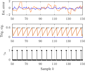
The estimation errors of the local and remote estimator are compared in the first graph. As expected, the remote estimation error (orange) is larger than the local estimation error (blue). Yet, the remote estimator only needs 14% of the samples.
The triggering behavior is illustrated in the second graph showing the triggering signals (43), (44), and , and the bottom graph depicting the triggering decision . Obviously, the ST entirely depends on the variance signal (orange, identical with in black), while (blue). This reflects the previous discussion about the ST being independent of online measurement data. The triggering behavior (the signal and the decisions ) is actually periodic, which can be deduced as follows: the variance of the KF (3)–(7) converges exponentially to a steady-state solution , [38]; hence, the triggering law (36) asymptotically becomes with , and (36) thus has a unique solution corresponding to the period seen in Fig. 4.
VI-B Predictive trigger
The results of simulating Example 1, now with the PT (38), (39), and prediction horizon , are presented in Fig. 5 for the cost , and in Fig. 6 for . Albeit using the same trigger, the two simulations show fundamentally different triggering behavior: while the triggering signal and the decisions in Fig. 5 are irregular, they are periodic in Fig. 6.
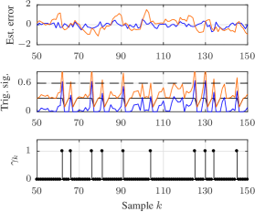
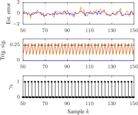
Apparently, the choice of the cost determines the different behavior of the PT. For , the triggering decision depends on both, the mean signal and the variance signal , as can be seen from Fig. 5 (middle graph). Because is based on real-time measurements, which are themselves random variables (2), the triggering decision is a random variable. We also observe in Fig. 5 that the variance signal is alone not sufficient to trigger a communication. However, when lowering the cost of communication enough, the variance signal alone becomes sufficient to cause triggers. Essentially, triggering then happens according to (39) only, and (38) becomes irrelevant. Hence, the PT resorts to self triggering behavior for small enough communication cost . That is, the PT undergoes a phase transition for some value of from stochastic/online triggering to deterministic/offline triggering behavior.
VI-C Estimation versus communication trade-off
Following the approach from [17], we evaluate the effectiveness of different triggers by comparing their trade-off curves of average estimation error versus average communication obtained from Monte Carlo simulations. In addition to the ST (36) and the PT (38), (39), , we also compare against the ET (41). The latter is expected to yield the best trade-off because it makes the triggering decision at the latest possible time (ET decides at time about communication at time ).
The estimation error is measured as the squared error averaged over the simulation horizon (200 samples) and simulation runs. The average communication is normalized such that means for all , and means no communication (except for one enforced trigger at ). By varying the constant communication cost in a suitable range, an -vs- curve is obtained, which represents the estimation/communication trade-off for a particular trigger. The results for Example 1 are shown in Fig. 7.
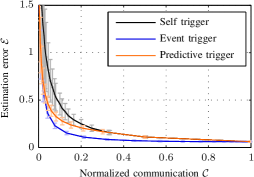
Comparing the three different triggering schemes, we see that the ET is superior, as expected, because its curve is uniformly below the others. Also expected, the ST is the least effective since no real-time information is available and triggers are purely based on variance predictions. The novel concept of predictive triggering can be understood as an intermediate solution between these two extremes. For small communication cost (and thus relatively large communication ), the PT behaves like the ST, as was discussed in the previous section and is confirmed in Fig. 7 (orange and black curves essentially identical for large ). When the triggering threshold is relaxed (i.e., the cost increased), the PT also exploits real-time data for the triggering decision (through (43)), similar to the ET. Yet, the PT must predict the decision steps in advance making its -vs- trade-off generally less effective than the ET. In Fig. 7, the curve for PT is thus between ET and ST and approaches either one of them for small and large communication .
VII Hardware Experiments: Remote Estimation & Feedback Control
Experimental results of applying the proposed PT and ST on an inverted pendulum platform are presented in this section. We show that trade-off curves in practice are similar to those in simulation (cf. Fig. 7), and that the triggers are suitable for feedback control (i.e., stabilizing the pendulum).
VII-A Experimental setup
The experimental platform used for the experiments of this section is the inverted pendulum system shown in Fig. 8. Through appropriate horizontal motion, the cart can stabilize the pendulum in its upright position (). The system state is given by the position and velocity of the cart, and angle and angular velocity of the pole, i.e., . The cart-pole system is widely used as a benchmark in control [42] because it has nonlinear, fast, and unstable dynamics.
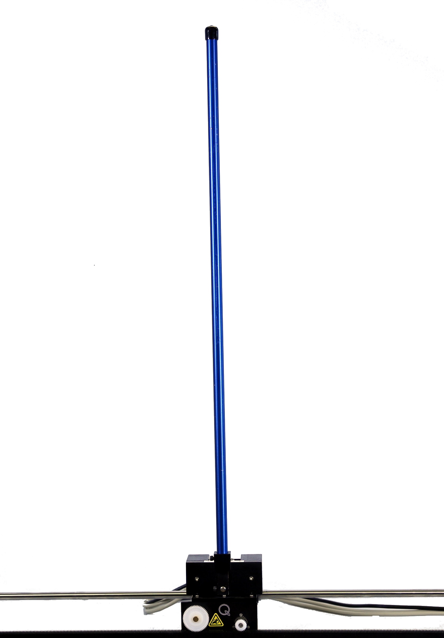

The sensors and actuator of the pendulum hardware are connected through data acquisition devices to a standard laptop running Matlab/Simulink. Two encoders measure the angle and cart position every ; and voltage is commanded to the motor with the same update interval. The full state can be constructed from the sensor measurements through finite differences. The triggers, estimators, and controllers are implemented in Simulink. The pendulum system thus represents one ‘Thing ’ of Fig. 1.
As the upright equilibrium is unstable, a stabilizing feedback controller is needed. We employ a linear-quadratic regulator (LQR), which is a standard design for multivariate feedback control, [43]. Assuming linear dynamics (with a model as given in [44]) and perfect state measurements, a linear state-feedback controller, , is obtained as the optimal feedback controller that minimizes a quadratic cost function
| (49) |
The positive definite matrices and are design parameters, which represent the designer’s trade-off in achieving a fast response (large ) or low control energy (large ). Here, we chose and with the identity matrix, which leads to stable balancing with slight motion of the cart. Despite the true system being nonlinear and state measurements not perfect, LQR leads to good balancing performance, which has also been shown in previous work on this platform [45].
Characteristics of the communication network to be investigated are implemented in the Simulink model. The round time of the network is assumed to be . For the PT, the prediction horizon is . Thus, the communication network has to reconfigure, which is expected to be sufficient for fast protocols such as [40].
VII-B Remote estimation
The first set of experiments investigates the remote estimation scenario as in Fig. 3. For this purpose, the pendulum is stabilized locally via the above LQR, which runs at and directly acts on the encoder measurements and their derivatives obtained from finite differences. The closed-loop system thus serves as the dynamic process in Fig. 3 (described by equation (1)), whose state is to be estimated and communicated via ET, PT, and ST to a remote location, which could represent another agent from Fig. 1.
The local State Estimator in Fig. 3 is implemented as the KF (3)–(7) with properly tuned matrices and updated every (at every sensor update). Triggering decisions are made at the round time of the network (). Accordingly, state predictions (14) are made every (in Prediction Thing in Fig. 3).
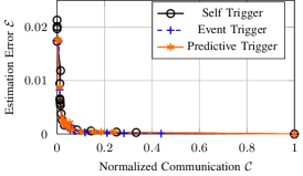
Analogously to the numerical examples in Sec. VI, we investigate the estimation-versus-communication trade-off achieved by ET, PT, and ST. As can be seen in Fig. 9, all three triggers lead to approximately the same curves. These results are qualitatively different from those of the numerical example in Fig. 7, which showed notable differences between the triggers. Presumably, the reason for this lies in the low-noise environment of this experiment. The main source of disturbances is the encoder quantization, which is negligible. Therefore, the system is almost deterministic, and predictions are very accurate. Hence, in this setting, predicting future communication needs (PT, ST) does not involve any significant disadvantage compared to instantaneous decisions (ET).
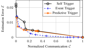
To confirm these results, we added zero-mean Gaussian noise with variance to the position and angle measurements. This emulates analog angle sensors instead of digital encoders and is representative for many sensors in practice that involve stochastic noise. The results of this experiment are shown in Fig. 10, which shows the same qualitative difference between the triggers as was observed in the numerical example in Fig. 7.
VII-C Feedback control
The estimation errors obtained in Fig. 9 are fairly small even with low communication. Thus, we expect the estimates obtained with PT and ST also to be suitable for feedback control, which we investigate here. In contrast to the setting in Sec. VII-B, the LQR controller does not use the local state measurements at the fast update interval of , but the state predictions (14) instead. This corresponds to the controller being implemented on a remote agent, which is relevant for IoT control as in Fig. 1, where feedback loops are closed over a resource-limited network.
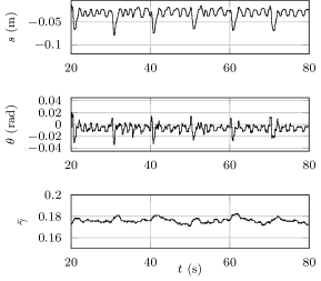
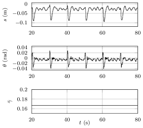
Figures 11 and 12 show experimental results of using PT and ST for feedback control. For these experiments, the weights of the LQR approach were chosen as those suggested by the manufacturer in [44], which leads to a slightly more robust controller. Both triggers are able to stabilize the pendulum well and save around of communication.
In addition to disturbances inherent in the system, the experiments also include impulsive disturbances on the input (impulse of amplitude and duration every ), which we added to study the triggers’ behavior under deterministic disturbances. In addition to stochastic noise, such disturbances are relevant in many practical IoT scenarios (e.g., a car braking, a wind gust on a drone). Under these disturbances, a particular advantage of PT over ST becomes apparent. The ST is an offline trigger, which yields periodic communication (in this setting) and does not react to the external disturbances. The PT, on the other hand, takes the current error into account and is thus able to issue additional communication in case of disturbances. As a result, the maximum angle of the pendulum stays around in magnitude for the PT, while it comes close to for the ST.
VIII IoT Control with Multiple Agents
In the preceding sections, we addressed the problem posed in Sec. III-F for the case of two agents. In this section, we discuss how these results can be used for the IoT scenario with multiple agents in Fig. 1. Moreover, we sketch how the resulting closed-loop dynamics can be analyzed when remote estimates are used for feedback control.
Because we discuss multiple agents, we reintroduce the index ‘’ to refer to an individual agent from here onward.
VIII-A Multiple agents
The developments for a pair of agents as in Fig. 2 in the previous sections equally apply to the IoT scenario in Fig. 1. Each agent implements the blocks from Fig. 2: State Estimation is given by the KF (3)–(7), Prediction by (14), Control by (10), and the Event Trigger is replaced by either the ST (36) or the PT (38), (39). In particular, each agent makes predictions for those other agents whose state it requires for coordination. Whenever one agent transmits its local state estimate, it is broadcast over the network and received by all agents that care about this information, e.g., via many-to-all communication. In the considered scenario, the dynamics of the things are decoupled according to (1), (2) (cf. Fig. 1), but their action is coupled through the cooperative control (10).
In Sec. IX, a simulation study of an IoT control problem with multiple agents is discussed.
VIII-B Closed-loop analysis
While the main object of study in this article are predictive and self triggering for state estimation (cf. Fig. 3), an important use of the algorithms is for feedback control as in Fig. 1 and 2. The general suitability of the algorithms for feedback control has already been demonstrated in Sec. VII-C. As for feedback control, analyzing the closed-loop dynamics (e.g., for stability) is often of importance, we briefly outline here how this can be approached.
The closed-loop state dynamics of agent are obtained from (1) and (10), and can be rewritten as
| (50) |
where is the KF estimation error (9) and the remote estimation error (15). The combined closed-loop dynamics of things with concatenated state can then be written as
| (51) |
where
denotes block-diagonal matrix, and , , and are the combined vectors of all , , and (), respectively. The ‘tilde’ notation indicates variables that refer to the ensemble of all agents.
Equation (51) describes the closed-loop dynamics of things of Fig. 1 that implement the control architecture in Fig. 2; it can therefore be used to deduce closed-loop system properties. The evolution of the complete state is governed by the transition matrix and driven by three input terms: the KF error , the remote error , and process noise . Under mild assumptions, the feedback matrix can be designed such that a stable transition matrix results (i.e., all eigenvalues with magnitude less than 1), which implies that is exponentially stable. Stability analysis then amounts to showing that the input terms are well behaved and bounded in a stochastic sense (e.g., bounded moments).222For example, if, in , the input is uncorrelated and Gaussian with bounded variance, then stability of implies bounded state variance (see, e.g., [38, Sec. 4.3]). While is Gaussian by assumption (cf. Sec. III-A), being Gaussian follows from standard KF analysis [38] (cf. Sec. III-B). Lemmas 1 and 2 can be instrumental to analyze the distribution of . However, the distribution of depends on the chosen trigger, and its properties (e.g., bounded second moment) would have to be formally shown, which is beyond the goals of this article.
IX Simulation Study: Vehicle Platooning
To illustrate the scalability of the proposed triggers for IoT control, we present a simulation study of vehicle platooning. Connected vehicles are seen as a building block of the Internet of Vehicles [46]. Platooning of autonomous vehicles has been extensively studied in literature, e.g., for heavy-duty freight transport [47, 48]. It has been shown that platooning leads to remarkable improvements in terms of fuel consumption.
IX-A Model
We consider a chain of vehicles (see Fig. 13), which are modeled as unit point masses (cf. [49, 15]). The state of each vehicle is its absolute position and velocity , and its acceleration is the control input. The control objectives are to maintain a desired distance between the vehicles and track a desired velocity for the platoon. For this study, we assume that every vehicle measures its absolute position.

The architecture of the vehicle platoon is as in Fig. 1. To control the inter-vehicle distances, communication between the vehicles is required. We thus implement the IoT control architecture given by Fig. 2 with PT and ST to save communication. We assume as the sample time for the inter-vehicle communication. Here, we consider the case where each vehicle transmits its local state information to all other vehicles. Alternative architectures, where communication is only possible with a subset of vehicles, are also conceivable in the considered scenario (see [48]), and the PT and ST can be used for only the required communication links appropriately.
For our chosen setup, where each vehicle is only able to measure its own absolute position, it is obvious that communication between vehicles is necessary to control the inter-vehicle distance. However, even if local sensor measurements are available, e.g., if every vehicle can measure the distance to the preceding vehicle via a radar sensor, communication is required to guarantee string stability. String stability indicates whether oscillations are amplified upstream the traffic flow. In [50], it has been proven that if only local sensor measurements are used, string stability can only be guaranteed for velocity dependent spacing policies, i.e., the faster the cars drive the larger distances are required, and thus, the less fuel can be saved. Therefore, even in the presence of local measurements, communication between vehicles is crucial for fuel saving. In such a case, where additional local sensor measurements are available, predictive and self triggering can similarly be used, as also stated in Remark 1.
To address the control objectives, we design an LQR for the linear state-space model that includes the vehicle velocities and their relative distances, i.e., . The complete state is given by except for no relative position for the last vehicle (cf. Fig. 13). For this system, an LQR is designed with and . The even-numbered diagonal entries of the matrix specify the inter-vehicle distance tracking, while the odd ones weight the desired velocity. To achieve tracking of desired velocity and inter-vehicle distance, the desired state is introduced, and the LQR law implemented.
We emphasize that the feedback gain matrix is dense; that is, information about all states in the platoon are used to compute the optimal control input. Such controller can only be implemented in a distributed way, if complete state information is available on each agent via the architecture presented in Sec. III-D with all-to-all communication.
In the simulations333The Python source code for the simulations is available under https://github.com/baumanndominik/predictive_and_self_triggering. below, position measurements are corrupted by independent noise, uniformly distributed in . Likewise, the inputs are corrupted by uniform noise in . Additionally, we assume Bernoulli packet drops.
IX-B Platooning on changing surfaces
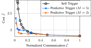
We investigate the performance versus communication trade-off achieved with PT and ST for platooning of vehicles. Here, we are interested in the closed-loop performance that is achieved with the proposed architecture; hence, instead of the estimation error, we use the sum of the absolute value of the error between and , normalized by the state dimension and number of time steps, as performance metric .444LQR cost as one alternative performance metric leads to similar insights, but may have higher variance. The platoon drives for , while keeping desired inter-vehicle distances of and velocity of . After , the dynamics change due to different road conditions (e.g., continue driving on a wet road after leaving a tunnel), which is modeled by altering the vehicle dynamics accordingly (vehicles moving faster, and the effect of braking/accelerating is reduced by ). Fig. 14 shows the results from Monte Carlo simulations.
Both triggers achieve significant communication savings at only a mild decrease of control performance. Similar to studies in previous sections, the PT performs better than the ST for low communication rates, because it can react to changing conditions. For high communication rates, PT and ST are identical. If the prediction horizon is extended, the performance of the PT gets closer to that of the ST, as can be obtained from the blue curve in Fig. 14.
IX-C Braking
If vehicles drive in close proximity, the ability to react to sudden changes, such as a braking maneuver of the preceding car, is critical. This is investigated here for three vehicles (simulation with more vehicles leads to the same insight).
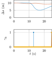
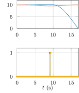
Figure 15 shows simulation results, where all cars start with a velocity of , but after , the first car brakes. The results in Fig. 15 (left) show that even with very little communication, the PT is able to deal with this situation. The PT detects the need for more communication and is able to control inter-vehicle distances within safety bounds. As previously pointed out, the ST (Fig. 15 right) cannot react online, which causes a crash in this example ().
X Conclusion
In IoT control, feedback loops are closed between multiple things over a general-purpose network. Since the network is shared by many entities, communication is a limited resource that must be taken into account for optimal system-level operation when making control decisions. This work sets a foundation for such resource-aware IoT control. Distributed event-based state estimation (DEBSE) provides a powerful architecture for sharing information between multiple things and their cooperative control. The developed self trigger and predictive trigger allow one to anticipate future communication needs, which is fundamental for efficiently (re-)allocating network resources.
In order to leverage the potential of this work and realize actual resource savings on concrete IoT systems, the integration of ST and PT herein with a suitable communication system is essential. While DEBSE has successfully been implemented on wired CAN bus networks in prior works [12, 14], we target the integration with modern wireless network protocols such as the Low-power Wireless Bus (LWB) [40] in ongoing work. LWB essentially abstracts a multi-hop wireless network as a common bus enabling fast [51] and reliable [52] many-to-all communication. Hence, it is ideally suited for scenarios such as in Figures 1 and 2, where multiple things require information about each other for coordination. In particular, all-to-all communication allows for the effective realization of the predictors (14) on any agent that needs the corresponding state information. LWB typically runs a network manager on one of its nodes, which can use the communication requirements signaled by ST and PT to schedule next communication rounds. The concrete development and integration of such schemes is subject of ongoing research. While the focus of this article is on saving communication bandwidth, the proposed triggers can also be instrumental for saving other resources in IoT (e.g., computation or energy).
The predictive and self triggers are suitable for different application scenarios. The simulation and experimental studies herein clearly highlight the advantage of the predictive trigger: by continuously monitoring the triggering condition, it can react to unforeseeable events such as disturbances. The self trigger, on the other hand, is an offline trigger, which allows for setting devices to sleep. In contrast to commonly used event triggers, both proposed triggers can predict resource needs rather than making instantaneous decisions. Predictive triggering is a novel concept in-between the previously proposed concepts of self triggering and event triggering.
Concrete instances of the predictive and self trigger were derived herein for estimation of linear Gaussian systems. While the general idea of predicting triggers also extends to nonlinear estimation, properly formalizing this and deriving triggering laws for nonlinear problems is an interesting task for future work. Likewise, considering alternative optimization problems for different error choices in (16), as well as dynamic programming formulations in place of the one-step optimization in (17), may lead to interesting insights and alternative triggers. While the predictive and self triggers herein were shown to stabilize the inverted pendulum in the reported experiments, formally analyzing stability of the closed-loop system (e.g., along the lines outlined in Sec. VIII-B) is another relevant open research question.
Appendix A Proof of Lemma 1
Because for from (14), the remote error is identical to the KF error . From KF theory [38, p. 41], it is known that the conditional and unconditional error distributions are identical, namely
| (52) |
That is, the error distribution is independent of any measurement data. Therefore, we also have (see [18, Proof of Lem. 2] for a formal argument), from which the claim follows with (52).
Appendix B Proof of Lemma 2
We first establish, for any ,
| (53) | ||||
| (54) |
with the KF innovation, the KF gain, and as in (29), through proof by induction. For , (53) and (54) hold trivially with and , respectively. Induction assumption (IA): assume (53) and (54) hold for . Show they are then also true for . We have from the KF iterations:
and
Hence, (53) and (54) are true for , which completes the induction.
Next, we analyze the error for the case (no communication). To ease the presentation, we introduce the auxiliary variable .
Case (i): First, we note that implies because , the last nonzero element of , is in the past, and the identity thus follows from the definition of . It follows further that all triggering decisions following are 0 until (otherwise would not be the last element in ). Hence, we have the communication pattern and .
Let . From
it follows that the conditional distribution (24) is Gaussian. It thus suffices to consider mean and variance in the following.
For the conditional mean, we have
| (55) |
and
| (56) |
where we used the tower property of conditional expectation, (8), and (54) with the fact that the KF innovation sequence is zero-mean and uncorrelated. Using (56) with (55), we obtain
| (57) | |||
| (58) |
which proves (25). The first and third sum in (57) can be seen to be identical by substituting with .
Employing the tower property for the conditional variance, we get
Furthermore, follows from (54), being uncorrelated, and
as defined in (28). This completes the proof for Case (i).
Case (ii): We use to simplify notation. By definition of , we have , and hence . That is, a triggering will happen now or before the end of the horizon . At the triggering instant , we have from (14), . Hence, the distribution of the error at time is known irrespective of past and future data. Following the same arguments as in the proof of Lemma 1, we have .
Acknowledgment
The authors thank their colleagues Felix Grimminger and Alonso Marco for their support with the experimental setup and Friedrich Solowjow for insightful discussions.
References
- [1] L. Atzori, A. Iera, and G. Morabito, “The Internet of Things: A survey,” Computer Networks, vol. 54, no. 15, pp. 2787–2805, 2010.
- [2] J. Gubbi, R. Buyya, S. Marusic, and M. Palaniswami, “Internet of Things (IoT): A vision, architectural elements, and future directions,” Future Generation Computer Systems, vol. 29, no. 7, pp. 1645–1660, 2013.
- [3] T. Samad, “Control systems and the internet of things [technical activities],” IEEE Control Systems, vol. 36, no. 1, pp. 13–16, Feb 2016.
- [4] J. Lunze, Control theory of digitally networked dynamic systems. Springer, 2014.
- [5] J. P. Hespanha, P. Naghshtabrizi, and Y. Xu, “A survey of recent results in networked control systems,” Proceedings of the IEEE, vol. 95, no. 1, pp. 138–162, Jan. 2007.
- [6] K. J. Åström and B. Bernhardsson, “Comparison of periodic and event based sampling for first-order stochastic systems,” in Proc. of the 14th IFAC World Congress, 1999, pp. 301–306.
- [7] K. Årzén, “A simple event-based PID controller,” in Proc. of the 14th IFAC World Congress, 1999, pp. 423–428.
- [8] M. Lemmon, “Event-triggered feedback in control, estimation, and optimization,” in Networked Control Systems, ser. Lecture Notes in Control and Information Sciences, A. Bemporad, M. Heemels, and M. Johansson, Eds. Springer, 2010, vol. 406, pp. 293–358.
- [9] W. P. M. H. Heemels, K. H. Johansson, and P. Tabuada, “An introduction to event-triggered and self-triggered control,” in 51st IEEE Conference on Decision and Control, 2012, pp. 3270–3285.
- [10] M. Miskowicz, Event-Based Control and Signal Processing. CRC Press, 2016.
- [11] D. Shi, L. Shi, and T. Chen, Event-Based State Estimation. Springer, 2016.
- [12] S. Trimpe and R. D’Andrea, “An experimental demonstration of a distributed and event-based state estimation algorithm,” in 18th IFAC World Congress, 2011, pp. 8811–8818.
- [13] ——, “Event-based state estimation with variance-based triggering,” IEEE Transaction on Automatic Control, vol. 59, no. 12, pp. 3266–3281, 2014.
- [14] S. Trimpe, “Event-based state estimation: an emulation-based approach,” IET Control Theory & Applications, vol. 11, pp. 1684–1693, July 2017.
- [15] M. Muehlebach and S. Trimpe, “Distributed event-based state estimation for networked systems: An LMI-approach,” IEEE Transactions on Automatic Control, vol. 63, no. 1, pp. 269–276, Jan. 2018.
- [16] J. Araújo, M. Mazo Jr, A. Anta, P. Tabuada, and K. H. Johansson, “System architectures, protocols and algorithms for aperiodic wireless control systems,” IEEE Transactions on Industrial Informatics, vol. 10, no. 1, pp. 175–184, Feb 2014.
- [17] S. Trimpe and M. Campi, “On the choice of the event trigger in event-based estimation,” in International Conference on Event-based Control, Communication, and Signal Processing, 2015, pp. 1–8.
- [18] S. Trimpe, “Predictive and self triggering for event-based state estimation,” in 55th IEEE Conference on Decision and Control, Dec. 2016, pp. 3098–3105.
- [19] J. Sijs, B. Noack, M. Lazar, and U. D. Hanebeck, “Time-periodic state estimation with event-based measurement updates,” in Event-Based Control and Signal Processing. CRC Press, 2016.
- [20] M. Martínez-Rey, F. Espinosa, A. Gardel, and C. Santos, “On-board event-based state estimation for trajectory approaching and tracking of a vehicle,” Sensors, vol. 15, no. 6, pp. 14 569–14 590, 2015.
- [21] J. Sijs, B. Noack, and U. Hanebeck, “Event-based state estimation with negative information,” in 16th International Conference on Information Fusion, 2013, pp. 2192–2199.
- [22] D. Shi, T. Chen, and L. Shi, “An event-triggered approach to state estimation with multiple point- and set-valued measurements,” Automatica, vol. 50, no. 6, pp. 1641–1648, 2014.
- [23] J. Wu, Q.-S. Jia, K. Johansson, and L. Shi, “Event-based sensor data scheduling: Trade-off between communication rate and estimation quality,” IEEE Transactions on Automatic Control, vol. 58, no. 4, pp. 1041–1046, 2013.
- [24] A. S. Leong, S. Dey, and D. E. Quevedo, “Sensor scheduling in variance based event triggered estimation with packet drops,” IEEE Transactions on Automatic Control, vol. 62, no. 4, pp. 1880–1895, 2017.
- [25] J. Marck and J. Sijs, “Relevant sampling applied to event-based state-estimation,” in Int. Conf. on Sensor Technologies and Applications, Jul. 2010, pp. 618–624.
- [26] M. Velasco, J. Fuertes, and P. Marti, “The self triggered task model for real-time control systems,” in Work-in-Progress Session of the 24th IEEE Real-Time Systems Symposium, 2003.
- [27] X. Wang and M. Lemmon, “Self-triggered feedback control systems with finite-gain stability,” IEEE Transactions on Automatic Control, vol. 54, no. 3, pp. 452–467, 2009.
- [28] M. Mazo, A. Anta, and P. Tabuada, “An ISS self-triggered implementation of linear controllers,” Automatica, vol. 46, no. 8, pp. 1310–1314, 2010.
- [29] A. Anta and P. Tabuada, “To sample or not to sample: Self-triggered control for nonlinear systems,” IEEE Transactions on Automatic Control, vol. 55, no. 9, pp. 2030–2042, 2010.
- [30] N. Meslem and C. Prieur, “State estimation based on self-triggered measurements,” in 19th IFAC World Congress, 2014, pp. 86–91.
- [31] V. Andrieu, M. Nadri, U. Serres, and J.-C. Vivalda, “Self-triggered continuous-discrete observer with updated sampling period,” Automatica, vol. 62, pp. 106–113, 2015.
- [32] F. D. Brunner, T. M. P. Gommans, W. P. M. H. Heemels, and F. Allgöwer, “Resource-aware set-valued estimation for discrete-time linear systems,” in IEEE Conference on Decision and Control, 2015, pp. 5480–5486.
- [33] M. Kögel and R. Findeisen, “Robust output feedback predictive control with self-triggered measurements,” in IEEE Conference on Decision and Control, 2015, pp. 5487–5493.
- [34] J. Almeida, C. Silvestre, and A. M. Pascoal, “Observer based self-triggered control of linear plants with unknown disturbances,” in American Control Conference, 2012, pp. 5688–5693.
- [35] W. Wu and A. Arapostathis, “Optimal sensor querying: General markovian and LQG models with controlled observations,” IEEE Transactions on Automatic Control, vol. 53, no. 6, pp. 1392–1405, July 2008.
- [36] Y. Xu and J. P. Hespanha, “Optimal communication logics in networked control systems,” in IEEE Conference on Decision and Control, vol. 4, Dec 2004, pp. 3527–3532 Vol.4.
- [37] G. M. Lipsa and N. C. Martins, “Remote state estimation with communication costs for first-order lti systems,” IEEE Transactions on Automatic Control, vol. 56, no. 9, pp. 2013–2025, 2011.
- [38] B. D. O. Anderson and J. B. Moore, Optimal Filtering. Mineola, New York: Dover Publications, 2005.
- [39] J.-P. Thomesse, “Fieldbus technology in industrial automation,” Proceedings of the IEEE, vol. 93, no. 6, pp. 1073–1101, June 2005.
- [40] F. Ferrari, M. Zimmerling, L. Mottola, and L. Thiele, “Low-power wireless bus,” in ACM Conference on Embedded Network Sensor Systems, Toronto, Ontario, Canada, Nov. 2012, pp. 1–14.
- [41] F. Mager, D. Baumann, R. Jacob, L. Thiele, S. Trimpe, and M. Zimmerling, “Feedback control goes wireless: Guaranteed stability over low-power multi-hop networks,” in ACM/IEEE International Conference on Cyber-Physical Systems, 2019, accepted, preprint: arXiv:1804.08986.
- [42] O. Boubaker, “The inverted pendulum benchmark in nonlinear control theory: A survey,” International Journal of Advanced Robotic Systems, vol. 10, no. 5, p. 233, 2013.
- [43] B. Anderson and J. Moore, Optimal Control: Linear Quadratic Methods, ser. Dover Books on Engineering. Dover Publications, 2007.
- [44] Quanser Inc., “IP02 - self-erecting single inverted pendulum (SESIP) - linear experiment #6: PV and LQR control - instructor manual.”
- [45] A. Marco et al., “Virtual vs. real: Trading off simulations and physical experiments in reinforcement learning with bayesian optimization,” in IEEE International Conference on Robotics and Automation, May 2017.
- [46] N. Lu, N. Cheng, N. Zhang, X. Shen, and J. W. Mark, “Connected vehicles: Solutions and challenges,” IEEE Internet of Things Journal, vol. 1, no. 4, pp. 289–299, May 2014.
- [47] B. Besselink, V. Turri, S. H. van de Hoef, K. Y. Liang, A. Alam, J. Mårtensson, and K. H. Johansson, “Cyber-physical control of road freight transport,” Proceedings of the IEEE, vol. 104, no. 5, pp. 1128–1141, May 2016.
- [48] A. Alam, J. Mårtensson, and K. H. Johansson, “Experimental evaluation of decentralized cooperative cruise control for heavy-duty vehicle platooning,” Control Engineering Practice, vol. 38, pp. 11 – 25, 2015.
- [49] W. Levine and M. Athans, “On the optimal error regulation of a string of moving vehicles,” IEEE Transactions on Automatic Control, vol. 11, no. 3, pp. 355–361, Jul 1966.
- [50] G. J. Naus, R. P. Vugts, J. Ploeg, M. J. van de Molengraft, and M. Steinbuch, “String-stable cacc design and experimental validation: A frequency-domain approach,” IEEE Transactions on vehicular technology, vol. 59, no. 9, pp. 4268–4279, 2010.
- [51] M. Zimmerling, L. Mottola, P. Kumar, F. Ferrari, and L. Thiele, “Adaptive real-time communication for wireless cyber-physical systems,” ACM Transaction on Cyber-Physical Systems, vol. 1, no. 2, 2017.
- [52] F. Ferrari, M. Zimmerling, L. Thiele, and O. Saukh, “Efficient network flooding and time synchronization with Glossy,” in ACM/IEEE Int. Conf. on Information Processing in Sensor Networks, 2011.
![[Uncaptioned image]](/html/1901.07531/assets/x17.png) |
Sebastian Trimpe (M’12) received the B.Sc. degree in general engineering science and the M.Sc. degree (Dipl.-Ing.) in electrical engineering from Hamburg University of Technology, Hamburg, Germany, in 2005 and 2007, respectively, and the Ph.D. degree (Dr. sc.) in mechanical engineering from ETH Zurich, Zurich, Switzerland, in 2013. He is currently a Research Group Leader at the Max Planck Institute for Intelligent Systems, Stuttgart, Germany, where he leads the independent Max Planck Research Group on Intelligent Control Systems. His main research interests are in systems and control theory, machine learning, networked and autonomous systems. Dr. Trimpe is a recipient of the General Engineering Award for the best undergraduate degree (2005), a scholarship from the German National Academic Foundation (2002 to 2007), the triennial IFAC World Congress Interactive Paper Prize (2011), and the Klaus Tschira Award for public understanding of science (2014). |
![[Uncaptioned image]](/html/1901.07531/assets/Figures_Dominik/Dominik_Baumann_BW.png) |
Dominik Baumann received the Dipl.-Ing. degree in electrical engineering from TU Dresden, Germany, in 2016. He is currently a PhD student in the Intelligent Control Systems Group at the Max Planck Institute for Intelligent Systems, Tübingen, Germany. His research interests include control theory, robotics, distributed and cooperative control, learning and networked control systems. |