Lattice QCD determination of neutron-antineutron matrix elements with physical quark masses

Enrico Rinaldi erinaldi@bnl.gov RIKEN BNL Research Center, Brookhaven National Laboratory, Upton, NY 11973, USA Nuclear Science Division, Lawrence Berkeley National Laboratory, Berkeley, CA 94720, USA    Sergey Syritsyn sergey.syritsyn@stonybrook.edu RIKEN BNL Research Center, Brookhaven National Laboratory, Upton, NY 11973, USA Department of Physics and Astronomy, Stony Brook University, Stony Brook, NY 11794, USA    Michael L. Wagman mlwagman@mit.edu Center for Theoretical Physics, Massachusetts Institute of Technology, Cambridge, MA 02139, USA    Michael I. Buchoff Lawrence Livermore National Laboratory, Livermore, California 94550, USA    Chris Schroeder Lawrence Livermore National Laboratory, Livermore, California 94550, USA    Joseph Wasem Lawrence Livermore National Laboratory, Livermore, California 94550, USA
Abstract

Matrix elements of six-quark operators are needed to extract new physics constraints from experimental searches for neutron-antineutron oscillations. This work presents in detail the first lattice quantum chromodynamics calculations of the necessary neutron-antineutron transition matrix elements including calculation methods and discussions of systematic uncertainties. Implications of isospin and chiral symmetry on the matrix elements, power counting in the isospin limit, and renormalization of a chiral basis of six-quark operators are discussed. Calculations are performed with a chiral-symmetric discretization of the quark action and physical light quark masses in order to avoid the need for chiral extrapolation. Non-perturbative renormalization is performed, including a study of lattice cutoff effects. Excited-state effects are studied using two nucleon operators and multiple values of source-sink separation. Results for the dominant matrix elements are found to be significantly larger compared to previous results from the MIT bag model. Future calculations are needed to fully account for systematic uncertainties associated with discretization and finite-volume effects but are not expected to significantly affect this conclusion.

pacs:
preprint: MIT-CTP/5099, LLNL-JRNL-766337, RBRC-1305

I Introduction

In the contemporary theory of particles and fields, there is no fundamental reason for baryon number B𝐵B to be conserved. Quantum effects in the Standard Model (SM) can lead to B𝐵B violation, and at temperatures above the electroweak phase transition sphaleron processes can efficiently convert baryons into antileptons while preserving (BL)𝐵𝐿(B-L), where L𝐿L is lepton number. Low-temperature B𝐵B-violating effects have not been observed experimentally, and their existence would have significant implications for the stability of nuclear matter. However, the observed baryon-antibaryon asymmetry of the universe cannot be explained within the SM, which fulfills Sakharov’s conditions for baryogenesis Sakharov (1967) but does not contain enough baryon number and CP violation to reproduce the observed baryon asymmetry of the universe Cohen et al. (1993); Rubakov and Shaposhnikov (1996); Dine and Kusenko (2003); Canetti et al. (2012). Moreover, while (BL)𝐵𝐿(B-L) symmetry is preserved in the SM, it likely has to be violated in its extensions (BSM theories) aimed at explaining baryogenesis, since electroweak sphaleron transitions would otherwise “wash out” any net baryon number generated by (BL)𝐵𝐿(B-L)-conserving interactions in the early universe.

Baryon number violation might be experimentally observed in proton decays Miura (2016) or neutron-antineutron oscillations Baldo-Ceolin et al. (1994); Chung et al. (2002); Abe et al. (2015); Bergevin (2011). The implications of these two hypothetical processes are fundamentally different: proton decay changes baryon number by |ΔB|=1Δ𝐵1|\Delta B|=1 unit and involves (anti)leptons, while neutron-antineutron oscillations change baryon number by |ΔB|=2Δ𝐵2|\Delta B|=2 units and do not involve leptons. Proton decay, even if observed, does not necessarily violate (BL)𝐵𝐿(B-L) and may be insufficient to explain baryogenesis.

Despite decades of searches, neither process has been observed, constraining the strength of B𝐵B-violating interactions. In particular models of baryogenesis, this may require higher level of CP𝐶𝑃CP violation, which is in turn constrained by searches for the electric dipole moments of neutrons, nuclei, and atoms. However, excluding theories of baryogenesis using results from these experiments requires knowledge of nucleon matrix elements of B𝐵B- and CP𝐶𝑃CP-violating effective interactions expressed in terms of fundamental fields, quarks and gluons. For neutron-antineutron transitions, these calculations have previously been performed using nucleon models Rao and Shrock (1982). Modern lattice QCD methods permit model-independent calculation of these matrix elements. This paper reports the first completely nonperturbative calculation of the neutron-antineutron transition matrix elements computed in lattice QCD with physical quark masses and chiral symmetry. In particular, we find that lattice QCD calculations result in substantially larger n-n¯𝑛-¯𝑛n\text{-}\overline{n} matrix elements compared to nucleon model calculations. Our findings imply that n-n¯𝑛-¯𝑛n\text{-}\overline{n} oscillation experiments should observe 1-2 orders of magnitude more oscillation events than was previously expected for the same BSM physics parameters.

This paper describes in detail our methodology for computing neutron-antineutron matrix elements of operators changing baryon number by |ΔB|=2Δ𝐵2|\Delta B|=2 units, which have already been reported in a short publication Rinaldi et al. (2019). In particular, the operator definitions, symmetry properties of their matrix elements, and their impact on phenomenology within SU(2)L×U(1)𝑆𝑈subscript2𝐿𝑈1SU(2)_{L}\times U(1)-symmetric extensions are discussed in Sec. II. The setup for our calculation of these matrix elements on a lattice is described in Sec. III. Extraction of ground-state matrix elements from lattice correlation functions and analysis of potential excited state contaminations are performed in Sec. IV. Nonperturbative renormalization and matching to the MS¯¯MS\overline{\text{MS}} scheme are described in Sec. V. The final results for n-n¯𝑛-¯𝑛n\text{-}\overline{n} matrix elements and their uncertainties are provided in Sec. VI. In Section VII, we discuss briefly the impact of our results in light of other potential sources of systematic uncertainties that are not controlled in our present calculation.

II Effective n-n¯𝑛-¯𝑛n\text{-}\overline{n} interactions

II.1 Chiral basis of n-n¯𝑛-¯𝑛n\text{-}\overline{n} operators

A complete basis of color-singlet, electrically-neutral six-quark operators with uudddd𝑢𝑢𝑑𝑑𝑑𝑑uudddd flavor structure can be constructed from operators of the form Chang and Chang (1980); Kuo and Love (1980); Rao and Shrock (1982, 1984); Caswell et al. (1983)

𝒪χ1χ2χ31=(uiTCPχ1uj)(dkTCPχ2dl)(dmTCPχ3dn)T{ij}{kl}{mn}(symm),𝒪χ1χ2χ32=(uiTCPχ1dj)(ukTCPχ2dl)(dmTCPχ3dn)T{ij}{kl}{mn}(symm),𝒪χ1χ2χ33=(uiTCPχ1dj)(ukTCPχ2dl)(dmTCPχ3dn)T[ij][kl]{mn}(asym)formulae-sequencesubscriptsuperscript𝒪1subscript𝜒1subscript𝜒2subscript𝜒3superscriptsubscript𝑢𝑖𝑇𝐶subscript𝑃subscript𝜒1subscript𝑢𝑗superscriptsubscript𝑑𝑘𝑇𝐶subscript𝑃subscript𝜒2subscript𝑑𝑙superscriptsubscript𝑑𝑚𝑇𝐶subscript𝑃subscript𝜒3subscript𝑑𝑛superscriptsubscript𝑇𝑖𝑗𝑘𝑙𝑚𝑛(symm)formulae-sequencesubscriptsuperscript𝒪2subscript𝜒1subscript𝜒2subscript𝜒3superscriptsubscript𝑢𝑖𝑇𝐶subscript𝑃subscript𝜒1subscript𝑑𝑗superscriptsubscript𝑢𝑘𝑇𝐶subscript𝑃subscript𝜒2subscript𝑑𝑙superscriptsubscript𝑑𝑚𝑇𝐶subscript𝑃subscript𝜒3subscript𝑑𝑛superscriptsubscript𝑇𝑖𝑗𝑘𝑙𝑚𝑛(symm)subscriptsuperscript𝒪3subscript𝜒1subscript𝜒2subscript𝜒3superscriptsubscript𝑢𝑖𝑇𝐶subscript𝑃subscript𝜒1subscript𝑑𝑗superscriptsubscript𝑢𝑘𝑇𝐶subscript𝑃subscript𝜒2subscript𝑑𝑙superscriptsubscript𝑑𝑚𝑇𝐶subscript𝑃subscript𝜒3subscript𝑑𝑛superscriptsubscript𝑇delimited-[]𝑖𝑗delimited-[]𝑘𝑙𝑚𝑛(asym)\begin{split}{\mathcal{O}}^{1}_{\chi_{1}\chi_{2}\chi_{3}}&=(u_{i}^{T}CP_{\chi_{1}}u_{j})(d_{k}^{T}CP_{\chi_{2}}d_{l})(d_{m}^{T}CP_{\chi_{3}}d_{n})T_{\{ij\}\{kl\}\{mn\}}^{\text{(symm)}}\,,\\ {\mathcal{O}}^{2}_{\chi_{1}\chi_{2}\chi_{3}}&=(u_{i}^{T}CP_{\chi_{1}}d_{j})(u_{k}^{T}CP_{\chi_{2}}d_{l})(d_{m}^{T}CP_{\chi_{3}}d_{n})T_{\{ij\}\{kl\}\{mn\}}^{\text{(symm)}}\,,\\ {\mathcal{O}}^{3}_{\chi_{1}\chi_{2}\chi_{3}}&=(u_{i}^{T}CP_{\chi_{1}}d_{j})(u_{k}^{T}CP_{\chi_{2}}d_{l})(d_{m}^{T}CP_{\chi_{3}}d_{n})T_{[ij][kl]\{mn\}}^{\text{(asym)}}\,\end{split} (1)

where quark spinor indices are implicitly contracted in the parentheses, the PL,R=12(1γ5)subscript𝑃𝐿𝑅12minus-or-plus1subscript𝛾5P_{L,R}=\frac{1}{2}(1\mp\gamma_{5}) are chiral projectors, and the quark color tensors T𝑇T are

T{ij}{kl}{mn}(symm)subscriptsuperscript𝑇(symm)𝑖𝑗𝑘𝑙𝑚𝑛\displaystyle T^{\text{(symm)}}_{\{ij\}\{kl\}\{mn\}} =εikmεjln+εjkmεiln+εilmεjkn+εjlmεikn=TS1S2S3,absentsubscript𝜀𝑖𝑘𝑚subscript𝜀𝑗𝑙𝑛subscript𝜀𝑗𝑘𝑚subscript𝜀𝑖𝑙𝑛subscript𝜀𝑖𝑙𝑚subscript𝜀𝑗𝑘𝑛subscript𝜀𝑗𝑙𝑚subscript𝜀𝑖𝑘𝑛superscript𝑇subscript𝑆1subscript𝑆2subscript𝑆3\displaystyle=\varepsilon_{ikm}\varepsilon_{jln}+\varepsilon_{jkm}\varepsilon_{iln}+\varepsilon_{ilm}\varepsilon_{jkn}+\varepsilon_{jlm}\varepsilon_{ikn}=T^{S_{1}S_{2}S_{3}}\,, (2)
T[ij][kl]{mn}(asym)subscriptsuperscript𝑇(asym)delimited-[]𝑖𝑗delimited-[]𝑘𝑙𝑚𝑛\displaystyle T^{\text{(asym)}}_{[ij][kl]\{mn\}} =εijmεkln+εijnεklm=TA1A2S3,absentsubscript𝜀𝑖𝑗𝑚subscript𝜀𝑘𝑙𝑛subscript𝜀𝑖𝑗𝑛subscript𝜀𝑘𝑙𝑚superscript𝑇subscript𝐴1subscript𝐴2subscript𝑆3\displaystyle=\varepsilon_{ijm}\varepsilon_{kln}+\varepsilon_{ijn}\varepsilon_{klm}=T^{A_{1}A_{2}S_{3}}\,, (3)

with Sisubscript𝑆𝑖S_{i}, Aisubscript𝐴𝑖A_{i} standing for the symmetrized and antisymmetrized pairs of color indices, respectively. These operators are identical in Euclidean and Minkowski spaces with the charge-conjugation spin matrix C𝐶C,111 To avoid confusion, throughout the paper we use Euclidean γ𝛾\gamma-matrices (γ,γ4)uc=(γ,γ4)uc=(iγ,γ0)subscript𝛾subscript𝛾4𝑢𝑐superscriptsubscript𝛾subscript𝛾4𝑢𝑐subscript𝑖𝛾subscript𝛾0(\vec{\gamma},\gamma_{4})_{\mathcal{E}uc}=(\vec{\gamma},\gamma_{4})_{\mathcal{E}uc}^{\dagger}=(-i\vec{\gamma},\gamma_{0})_{{\mathcal{M}}} satisfying γμ=γμsuperscriptsubscript𝛾𝜇subscript𝛾𝜇\gamma_{\mu}^{\dagger}=\gamma_{\mu}.

C=γ2γ4=C=CT=C,𝐶subscript𝛾2subscript𝛾4superscript𝐶superscript𝐶𝑇superscript𝐶C=\gamma_{2}\gamma_{4}=C^{*}=-C^{T}=-C^{\dagger}\,, (4)

that satisfies the usual condition CγμC=γμT𝐶subscript𝛾𝜇superscript𝐶superscriptsubscript𝛾𝜇𝑇C\gamma_{\mu}C^{\dagger}=-\gamma_{\mu}^{T}. Operators involving vector diquarks (qTCPχγμq)superscript𝑞𝑇𝐶subscript𝑃𝜒subscript𝛾𝜇𝑞(q^{T}CP_{\chi}\gamma_{\mu}q) or tensor diquarks (qCPχσμνq)𝑞𝐶subscript𝑃𝜒subscript𝜎𝜇𝜈𝑞(qCP_{\chi}\sigma_{\mu\nu}q) are redundant and can be related to linear combinations of the operators in Eq. (1) by spin Fierz relations. The two choices of chirality for each (qCPχq)𝑞𝐶subscript𝑃𝜒𝑞(qCP_{\chi}q) diquark above in 𝒪1,2,3superscript𝒪123{\mathcal{O}}^{1,2,3} provide an overcomplete basis of 18 operators. Fierz relations 𝒪χχχ2𝒪χχχ1=3𝒪χχχ3subscriptsuperscript𝒪2𝜒𝜒superscript𝜒subscriptsuperscript𝒪1𝜒𝜒superscript𝜒3subscriptsuperscript𝒪3𝜒𝜒superscript𝜒{\mathcal{O}}^{2}_{\chi\chi\chi^{\prime}}-{\mathcal{O}}^{1}_{\chi\chi\chi^{\prime}}=3{\mathcal{O}}^{3}_{\chi\chi\chi^{\prime}} reduce the number of independent operators to 14.222 These Fierz relations are valid in four spacetime dimensions but are violated in dimensional regularization at two-loop order Buchoff and Wagman (2016). The MS¯¯MS\overline{\text{MS}} scheme defined in Ref. Buchoff and Wagman (2016) includes evanescent operator counterterms that ensure that renormalized matrix elements obey these Fierz relations. Provided that matching between BSM theory and SM effective operators is consistently performed in this MS¯¯MS\overline{\text{MS}} scheme or is performed at a high enough scale that one-loop QCD corrections are negligible, these Fierz relations can be assumed for MS¯¯MS\overline{\text{MS}} renormalized matrix elements.

All 14 independent effective six-quarks operators are electrically neutral and change the baryon number by ΔB=2Δ𝐵2\Delta B=-2 units. However, they are not independent under isospin symmetry transformations. The electroweak (EW) symmetry SU(2)L×U(1)Y𝑆𝑈subscript2𝐿𝑈subscript1𝑌SU(2)_{L}\times U(1)_{Y} requires that all interactions are SU(2)L𝑆𝑈subscript2𝐿SU(2)_{L}-singlet, which may be achieved with with additional factors of the Higgs field (see Sec.II.5). Furthermore, since the chiral symmetry SU(2)LSU(2)Rtensor-product𝑆𝑈subscript2𝐿𝑆𝑈subscript2𝑅SU(2)_{L}\otimes SU(2)_{R} is preserved exactly in the massless perturbation theory, and preserved with good precision on a lattice with chiral fermions, it is more convenient to use a basis made of operators having definite values of chiral L,R𝐿𝑅L,R-isospin.

The operators in Eq. (1) are built from color-symmetric (𝟔csubscript6𝑐\mathbf{6}_{c}) and antisymmetric (𝟑¯csubscript¯3𝑐\mathbf{\bar{3}}_{c}) chiral diquarks, which can be denoted as

(q1TCq2)χS,A=(q1TCPχq2)S,A=±(q2TCPχq1)S,Asubscriptsuperscriptsuperscriptsubscript𝑞1𝑇𝐶subscript𝑞2𝑆𝐴𝜒superscriptsuperscriptsubscript𝑞1𝑇𝐶subscript𝑃𝜒subscript𝑞2𝑆𝐴plus-or-minussuperscriptsuperscriptsubscript𝑞2𝑇𝐶subscript𝑃𝜒subscript𝑞1𝑆𝐴(q_{1}^{T}Cq_{2})^{S,A}_{\chi}=(q_{1}^{T}CP_{\chi}q_{2})^{S,A}=\pm(q_{2}^{T}CP_{\chi}q_{1})^{S,A} (5)

where q1,2=usubscript𝑞12𝑢q_{1,2}=u or d𝑑d and the relative signs upon quark permutation come from their anticommutation, CT=Csuperscript𝐶𝑇𝐶C^{T}=-C, and color (anti)symmetry. Using the isospin doublet ψ=(u,d)𝜓𝑢𝑑\psi=(u,d) and its conjugate ψ~=(ψTCiτ2)~𝜓superscript𝜓𝑇𝐶𝑖superscript𝜏2\tilde{\psi}=(\psi^{T}C\,i\tau^{2}), the chiral isoscalar and isovector diquarks can be written as

(ψ~ψ)χA,(ψ~τaψ)χS,subscriptsuperscript~𝜓𝜓𝐴𝜒subscriptsuperscript~𝜓superscript𝜏𝑎𝜓𝑆𝜒(\tilde{\psi}\psi)^{A}_{\chi}\,,\quad(\tilde{\psi}\tau^{a}\psi)^{S}_{\chi}\,, (6)

where τasuperscript𝜏𝑎\tau^{a} are the Pauli matrices, [τa,τb]=2iϵabcτcsuperscript𝜏𝑎superscript𝜏𝑏2𝑖superscriptitalic-ϵ𝑎𝑏𝑐superscript𝜏𝑐[\tau^{a},\tau^{b}]=2i\epsilon^{abc}\tau^{c}. The details of isospin classification were given in Ref. Buchoff and Wagman (2016), and here we list only the chiral-basis operators and their relation to the conventional basis (1). All the SU(2)L𝑆𝑈subscript2𝐿SU(2)_{L}-singlet operators can be constructed from some R𝑅R-diquarks and L𝐿L-isoscalar diquarks, resulting in three operators belonging to the (𝟏L,𝟑R)subscript1𝐿subscript3𝑅(\mathbf{1}_{L},\mathbf{3}_{R}) irreducible representation of the chiral isospin,

Q1=(ψ~ψ)RA1(ψ~ψ)RA2(ψ~τ+ψ)RS3TA1A2S3=4𝒪RRR3,Q2=(ψ~ψ)LA1(ψ~ψ)RA2(ψ~τ+ψ)RS3TA1A2S3=4𝒪LRR3,Q3=(ψ~ψ)LA1(ψ~ψ)LA2(ψ~τ+ψ)RS3TA1A2S3=4𝒪LLR3,formulae-sequencesubscript𝑄1subscriptsuperscript~𝜓𝜓subscript𝐴1𝑅subscriptsuperscript~𝜓𝜓subscript𝐴2𝑅subscriptsuperscript~𝜓superscript𝜏𝜓subscript𝑆3𝑅superscript𝑇subscript𝐴1subscript𝐴2subscript𝑆34subscriptsuperscript𝒪3𝑅𝑅𝑅subscript𝑄2subscriptsuperscript~𝜓𝜓subscript𝐴1𝐿subscriptsuperscript~𝜓𝜓subscript𝐴2𝑅subscriptsuperscript~𝜓superscript𝜏𝜓subscript𝑆3𝑅superscript𝑇subscript𝐴1subscript𝐴2subscript𝑆34subscriptsuperscript𝒪3𝐿𝑅𝑅subscript𝑄3subscriptsuperscript~𝜓𝜓subscript𝐴1𝐿subscriptsuperscript~𝜓𝜓subscript𝐴2𝐿subscriptsuperscript~𝜓superscript𝜏𝜓subscript𝑆3𝑅superscript𝑇subscript𝐴1subscript𝐴2subscript𝑆34subscriptsuperscript𝒪3𝐿𝐿𝑅\begin{split}Q_{1}&=(\tilde{\psi}\psi)^{A_{1}}_{R}\,(\tilde{\psi}\psi)^{A_{2}}_{R}\,(\tilde{\psi}\tau^{+}\psi)^{S_{3}}_{R}\,T^{A_{1}A_{2}S_{3}}=-4{\mathcal{O}}^{3}_{RRR}\,,\\ Q_{2}&=(\tilde{\psi}\psi)^{A_{1}}_{L}\,(\tilde{\psi}\psi)^{A_{2}}_{R}\,(\tilde{\psi}\tau^{+}\psi)^{S_{3}}_{R}\,T^{A_{1}A_{2}S_{3}}=-4{\mathcal{O}}^{3}_{LRR}\,,\\ Q_{3}&=(\tilde{\psi}\psi)^{A_{1}}_{L}\,(\tilde{\psi}\psi)^{A_{2}}_{L}\,(\tilde{\psi}\tau^{+}\psi)^{S_{3}}_{R}\,T^{A_{1}A_{2}S_{3}}=-4{\mathcal{O}}^{3}_{LLR}\,,\\ \end{split} (7)

and one (𝟏L,𝟕R)subscript1𝐿subscript7𝑅(\mathbf{1}_{L},\mathbf{7}_{R}) operator

Q4=[(ψ~τ3ψ)RS1(ψ~τ3ψ)RS215(ψ~τaψ)RS1(ψ~τaψ)RS2](ψ~τ+ψ)RS3TS1S2S3=45𝒪RRR1165𝒪RRR2,subscript𝑄4delimited-[]subscriptsuperscript~𝜓superscript𝜏3𝜓subscript𝑆1𝑅subscriptsuperscript~𝜓superscript𝜏3𝜓subscript𝑆2𝑅15subscriptsuperscript~𝜓superscript𝜏𝑎𝜓subscript𝑆1𝑅subscriptsuperscript~𝜓superscript𝜏𝑎𝜓subscript𝑆2𝑅subscriptsuperscript~𝜓superscript𝜏𝜓subscript𝑆3𝑅superscript𝑇subscript𝑆1subscript𝑆2subscript𝑆345subscriptsuperscript𝒪1𝑅𝑅𝑅165subscriptsuperscript𝒪2𝑅𝑅𝑅\begin{split}Q_{4}&=\Big{[}(\tilde{\psi}\tau^{3}\psi)^{S_{1}}_{R}\,(\tilde{\psi}\tau^{3}\psi)^{S_{2}}_{R}-\frac{1}{5}(\tilde{\psi}\tau^{a}\psi)^{S_{1}}_{R}\,(\tilde{\psi}\tau^{a}\psi)^{S_{2}}_{R}\Big{]}\,(\tilde{\psi}\tau^{+}\psi)^{S_{3}}_{R}\,T^{S_{1}S_{2}S_{3}}=-\frac{4}{5}{\mathcal{O}}^{1}_{RRR}-\frac{16}{5}{\mathcal{O}}^{2}_{RRR}\,,\end{split} (8)

where τ±=12(τ1±iτ2)superscript𝜏plus-or-minus12plus-or-minussuperscript𝜏1𝑖superscript𝜏2\tau^{\pm}=\frac{1}{2}(\tau^{1}\pm i\tau^{2}). The remaining 10 independent n-n¯𝑛-¯𝑛n\text{-}\overline{n} transition operators are not SU(2)L𝑆𝑈subscript2𝐿SU(2)_{L} singlets. Of these additional operators, three belong to the (𝟓L,𝟑R)subscript5𝐿subscript3𝑅(\mathbf{5}_{L},\mathbf{3}_{R}) irreducible representation,

Q5=(ψ~τψ)RS1(ψ~τ+ψ)LS2(ψ~τ+ψ)LS3TS1S2S3=𝒪RLL1,Q6=(ψ~τ3ψ)RS1(ψ~τ3ψ)LS2(ψ~τ+ψ)LS3TS1S2S3=4𝒪RLL2,Q7=[(ψ~τ3ψ)LS1(ψ~τ3ψ)LS213(ψ~τaψ)LS1(ψ~τaψ)LS2](ψ~τ+ψ)RS3TS1S2S3=43𝒪LLR183𝒪LLR2.formulae-sequencesubscript𝑄5subscriptsuperscript~𝜓superscript𝜏𝜓subscript𝑆1𝑅subscriptsuperscript~𝜓superscript𝜏𝜓subscript𝑆2𝐿subscriptsuperscript~𝜓superscript𝜏𝜓subscript𝑆3𝐿superscript𝑇subscript𝑆1subscript𝑆2subscript𝑆3subscriptsuperscript𝒪1𝑅𝐿𝐿subscript𝑄6subscriptsuperscript~𝜓superscript𝜏3𝜓subscript𝑆1𝑅subscriptsuperscript~𝜓superscript𝜏3𝜓subscript𝑆2𝐿subscriptsuperscript~𝜓superscript𝜏𝜓subscript𝑆3𝐿superscript𝑇subscript𝑆1subscript𝑆2subscript𝑆34subscriptsuperscript𝒪2𝑅𝐿𝐿subscript𝑄7delimited-[]subscriptsuperscript~𝜓superscript𝜏3𝜓subscript𝑆1𝐿subscriptsuperscript~𝜓superscript𝜏3𝜓subscript𝑆2𝐿13subscriptsuperscript~𝜓superscript𝜏𝑎𝜓subscript𝑆1𝐿subscriptsuperscript~𝜓superscript𝜏𝑎𝜓subscript𝑆2𝐿subscriptsuperscript~𝜓superscript𝜏𝜓subscript𝑆3𝑅superscript𝑇subscript𝑆1subscript𝑆2subscript𝑆343subscriptsuperscript𝒪1𝐿𝐿𝑅83subscriptsuperscript𝒪2𝐿𝐿𝑅\begin{split}Q_{5}&=(\tilde{\psi}\tau^{-}\psi)^{S_{1}}_{R}\,(\tilde{\psi}\tau^{+}\psi)^{S_{2}}_{L}\,(\tilde{\psi}\tau^{+}\psi)^{S_{3}}_{L}\,T^{S_{1}S_{2}S_{3}}={\mathcal{O}}^{1}_{RLL}\,,\\ Q_{6}&=(\tilde{\psi}\tau^{3}\psi)^{S_{1}}_{R}\,(\tilde{\psi}\tau^{3}\psi)^{S_{2}}_{L}\,(\tilde{\psi}\tau^{+}\psi)^{S_{3}}_{L}\,T^{S_{1}S_{2}S_{3}}=-4{\mathcal{O}}^{2}_{RLL}\,,\\ Q_{7}&=\Big{[}(\tilde{\psi}\tau^{3}\psi)^{S_{1}}_{L}\,(\tilde{\psi}\tau^{3}\psi)^{S_{2}}_{L}-\frac{1}{3}(\tilde{\psi}\tau^{a}\psi)^{S_{1}}_{L}\,(\tilde{\psi}\tau^{a}\psi)^{S_{2}}_{L}\Big{]}\,(\tilde{\psi}\tau^{+}\psi)^{S_{3}}_{R}\,T^{S_{1}S_{2}S_{3}}=-\frac{4}{3}{\mathcal{O}}^{1}_{LLR}-\frac{8}{3}{\mathcal{O}}^{2}_{LLR}\,.\end{split} (9)

The remaining seven independent operators Q1𝒫,,Q7𝒫superscriptsubscript𝑄1𝒫superscriptsubscript𝑄7𝒫Q_{1}^{\mathcal{P}},\cdots,Q_{7}^{\mathcal{P}} are obtained from Q1,,Q7subscript𝑄1subscript𝑄7Q_{1},\cdots,Q_{7} by parity transformation discussed below (35) and belong to the (𝟑L,𝟏R)subscript3𝐿subscript1𝑅(\mathbf{3}_{L},\mathbf{1}_{R}), (𝟕L,𝟏R)subscript7𝐿subscript1𝑅(\mathbf{7}_{L},\mathbf{1}_{R}), and (𝟑L,𝟓R)subscript3𝐿subscript5𝑅(\mathbf{3}_{L},\mathbf{5}_{R}) irreducible representations. The operators Q1,,Q7,Q1P,,Q7Psubscript𝑄1subscript𝑄7superscriptsubscript𝑄1𝑃superscriptsubscript𝑄7𝑃Q_{1},\cdots,Q_{7},Q_{1}^{P},\cdots,Q_{7}^{P} form a complete basis of 14 linearly independent SU(3)C×U(1)EM𝑆𝑈subscript3𝐶𝑈subscript1𝐸𝑀SU(3)_{C}\times U(1)_{EM}-invariant dimension-9 operators with baryon number ΔB=2Δ𝐵2\Delta B=-2 and isospin ΔI3=1Δsubscript𝐼31\Delta I_{3}=-1333 The isospin of operators ΔIQΔsubscript𝐼𝑄\Delta I_{Q} is defined here as [Q,I]=ΔIQQ𝑄𝐼Δsubscript𝐼𝑄𝑄[Q,\vec{I}]=\Delta\vec{I}_{Q}Q, leading to the selection rule IiIf=ΔIQsubscript𝐼𝑖subscript𝐼𝑓Δsubscript𝐼𝑄I_{i}-I_{f}=\Delta I_{Q} for the isospins of initial and final states. .

Table 1: Summary of operator properties and relations to notations used in other papers. The last column shows 1-loop QCD anomalous dimensions of the operators (see Sec. V).
QIsubscript𝑄𝐼Q_{I} Ref. Syritsyn et al. (2016) Ref. Rao and Shrock (1982) Ref. Grojean et al. (2018) (I,I3)R(I,I3)Ltensor-productsubscript𝐼subscript𝐼3𝑅subscript𝐼subscript𝐼3𝐿(I,I_{3})_{R}\otimes(I,I_{3})_{L} γ𝒪(0)superscriptsubscript𝛾𝒪0\gamma_{\mathcal{O}}^{(0)}
34Q134subscript𝑄1-\frac{3}{4}Q_{1} [(RRR)𝟏]delimited-[]subscript𝑅𝑅𝑅1\left[(RRR)_{\mathbf{1}}\right] 3𝒪{RR}R3=𝒪{RR}R2𝒪{RR}R13subscriptsuperscript𝒪3𝑅𝑅𝑅subscriptsuperscript𝒪2𝑅𝑅𝑅subscriptsuperscript𝒪1𝑅𝑅𝑅3{\mathcal{O}}^{3}_{\{RR\}R}={\mathcal{O}}^{2}_{\{RR\}R}-{\mathcal{O}}^{1}_{\{RR\}R} 12𝒪112subscript𝒪112{\mathcal{O}}_{1} (1,1)R(0,0)Ltensor-productsubscript11𝑅subscript00𝐿(1,-1)_{R}\otimes(0,0)_{L} 444
34Q234subscript𝑄2-\frac{3}{4}Q_{2} [(RR)𝟏L𝟎]delimited-[]subscript𝑅𝑅1subscript𝐿0\left[(RR)_{\mathbf{1}}L_{\mathbf{0}}\right] 3𝒪{LR}R3=𝒪{LR}R2𝒪{LR}R13subscriptsuperscript𝒪3𝐿𝑅𝑅subscriptsuperscript𝒪2𝐿𝑅𝑅subscriptsuperscript𝒪1𝐿𝑅𝑅3{\mathcal{O}}^{3}_{\{LR\}R}={\mathcal{O}}^{2}_{\{LR\}R}-{\mathcal{O}}^{1}_{\{LR\}R} 6𝒪26subscript𝒪26{\mathcal{O}}_{2} (1,1)R(0,0)Ltensor-productsubscript11𝑅subscript00𝐿(1,-1)_{R}\otimes(0,0)_{L} 44-4
34Q334subscript𝑄3-\frac{3}{4}Q_{3} [R𝟏(LL)𝟎]delimited-[]subscript𝑅1subscript𝐿𝐿0\left[R_{\mathbf{1}}(LL)_{\mathbf{0}}\right] 3𝒪{LL}R3=𝒪{LL}R2𝒪{LL}R13subscriptsuperscript𝒪3𝐿𝐿𝑅subscriptsuperscript𝒪2𝐿𝐿𝑅subscriptsuperscript𝒪1𝐿𝐿𝑅3{\mathcal{O}}^{3}_{\{LL\}R}={\mathcal{O}}^{2}_{\{LL\}R}-{\mathcal{O}}^{1}_{\{LL\}R} 12𝒪312subscript𝒪312{\mathcal{O}}_{3} (1,1)R(0,0)Ltensor-productsubscript11𝑅subscript00𝐿(1,-1)_{R}\otimes(0,0)_{L} 00
54Q454subscript𝑄4-\frac{5}{4}Q_{4} [(RRR)𝟑]delimited-[]subscript𝑅𝑅𝑅3[(RRR)_{\mathbf{3}}] 𝒪R{RR}1+4𝒪{RR}R2subscriptsuperscript𝒪1𝑅𝑅𝑅4subscriptsuperscript𝒪2𝑅𝑅𝑅{\mathcal{O}}^{1}_{R\{RR\}}+4{\mathcal{O}}^{2}_{\{RR\}R} (3,1)R(0,0)Ltensor-productsubscript31𝑅subscript00𝐿(3,-1)_{R}\otimes(0,0)_{L} +2424+24
Q5𝒫superscriptsubscript𝑄5𝒫-Q_{5}^{\mathcal{P}} [(RR)𝟐L𝟏](1)subscriptdelimited-[]subscript𝑅𝑅2subscript𝐿11\left[(RR)_{\mathbf{2}}L_{\mathbf{1}}\right]_{(1)} 𝒪L{RR}1subscriptsuperscript𝒪1𝐿𝑅𝑅{\mathcal{O}}^{1}_{L\{RR\}} 4𝒪4𝒫4superscriptsubscript𝒪4𝒫-4{\mathcal{O}}_{4}^{{\mathcal{P}}} (2,2)R(1,1)Ltensor-productsubscript22𝑅subscript11𝐿(2,-2)_{R}\otimes(1,1)_{L} +1212+12
14Q6𝒫14superscriptsubscript𝑄6𝒫\frac{1}{4}Q_{6}^{\mathcal{P}} [(RR)𝟐L𝟏](2)subscriptdelimited-[]subscript𝑅𝑅2subscript𝐿12\left[(RR)_{\mathbf{2}}L_{\mathbf{1}}\right]_{(2)} 𝒪{LR}R2subscriptsuperscript𝒪2𝐿𝑅𝑅{\mathcal{O}}^{2}_{\{LR\}R} 2𝒪5𝒫2superscriptsubscript𝒪5𝒫-2{\mathcal{O}}_{5}^{{\mathcal{P}}} (2,1)R(1,0)Ltensor-productsubscript21𝑅subscript10𝐿(2,-1)_{R}\otimes(1,0)_{L} +1212+12
34Q7𝒫34superscriptsubscript𝑄7𝒫\frac{3}{4}Q_{7}^{\mathcal{P}} [(RR)𝟐L𝟏](3)subscriptdelimited-[]subscript𝑅𝑅2subscript𝐿13\left[(RR)_{\mathbf{2}}L_{\mathbf{1}}\right]_{(3)} 𝒪R{RL}1+2𝒪{RR}L2subscriptsuperscript𝒪1𝑅𝑅𝐿2subscriptsuperscript𝒪2𝑅𝑅𝐿{\mathcal{O}}^{1}_{R\{RL\}}+2{\mathcal{O}}^{2}_{\{RR\}L} 4𝒪6𝒫4superscriptsubscript𝒪6𝒫-4{\mathcal{O}}_{6}^{{\mathcal{P}}} (2,0)R(1,1)Ltensor-productsubscript20𝑅subscript11𝐿(2,0)_{R}\otimes(1,-1)_{L} +1212+12

Isospin properties of the n-n¯𝑛-¯𝑛n\text{-}\overline{n} operators are summarized in Tab. 1, together with relations to notations used in other papers. In the following sections, we will discuss nucleon matrix elements only of the operators Q1,2,3,5subscript𝑄1235Q_{1,2,3,5}, and the other matrix elements can be easily obtained using symmetries discussed below.

II.2 Operator mixing

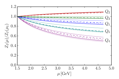
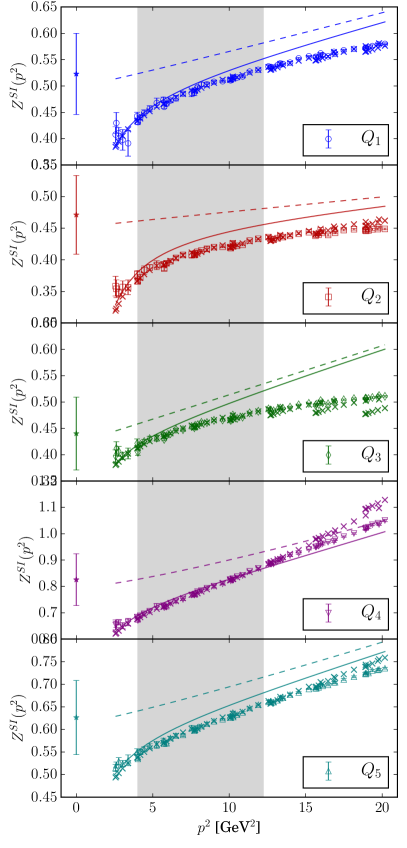
In this work, we study lattice regularized operators that have to be nonperturbatively renormalized and then perturbatively converted to the MS¯¯MS\overline{\text{MS}} scheme using the one-loop matching results of Ref. Buchoff and Wagman (2016), as described in Sec. V,

QIR(μ)=ZIJR(μ)QIlat.superscriptsubscript𝑄𝐼𝑅𝜇superscriptsubscript𝑍𝐼𝐽𝑅𝜇superscriptsubscript𝑄𝐼lat\begin{split}Q_{I}^{R}(\mu)=Z_{IJ}^{R}(\mu)Q_{I}^{\text{lat}}.\end{split} (10)

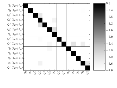
The renormalization matrix ZIJRsuperscriptsubscript𝑍𝐼𝐽𝑅Z_{IJ}^{R} takes especially simple form in the “chiral basis” consisting of elements QI=17(𝒫)superscriptsubscript𝑄𝐼17𝒫Q_{I=1\ldots 7}^{({\mathcal{P}})}, because they belong to different chiral multiplets and cannot mix with each other due to chiral SU(2)L×SU(2)R𝑆𝑈subscript2𝐿𝑆𝑈subscript2𝑅SU(2)_{L}\times SU(2)_{R} symmetry of massless QCD. Although some chiral representations appear in Tab. 1 more than once, they are actually also prevented from mixing. Specifically, operators Q5,6,7(𝒫)subscriptsuperscript𝑄𝒫567Q^{({\mathcal{P}})}_{5,6,7} consist of different components (“rows”) of chiral 𝟑3\mathbf{3}- and 𝟓5\mathbf{5}-multiplets, and transform differently under SU(2)L×SU(2)R𝑆𝑈subscript2𝐿𝑆𝑈subscript2𝑅SU(2)_{L}\times SU(2)_{R}. Operators Q1,2,3(𝒫)subscriptsuperscript𝑄𝒫123Q^{({\mathcal{P}})}_{1,2,3} cannot mix with each other for a more subtle reason. Even though they belong to the same chiral representation, they contain different numbers of left- and right-handed diquarks. While the U(1)A𝑈subscript1𝐴U(1)_{A} symmetry is violated in QCD by the ABJ anomaly, operators Q1,2,3subscript𝑄123Q_{1,2,3} do not mix in perturbative QCD because perturbative gluon exchanges preserve the U(1)A𝑈subscript1𝐴U(1)_{A} transformation properties of external quark fields in their respective Green’s functions. At the diagram level, there are only quark (and no antiquark) external fields, which cannot be contracted into closed loops, and thus penguin-like diagrams do not appear. This point is discussed and illustrated by an explicit two-loop perturbative calculation in Ref. Buchoff and Wagman (2016).

In order to avoid mixing of renormalized operators, one has to define renormalization matrix ZIJRsuperscriptsubscript𝑍𝐼𝐽𝑅Z_{IJ}^{R} in a scheme respecting chiral symmetry, such as MS¯¯MS\overline{\text{MS}}, and perform perturbative matching calculations in massless QCD. Likewise, to avoid mixing of bare lattice operators QIlatsuperscriptsubscript𝑄𝐼latQ_{I}^{\text{lat}}, chiral symmetry must be preserved in lattice QCD regularization, which requires [Möbius] domain wall ([M]DWF) or overlap fermion discretization. The MDWF action that we use in this work has been shown to have good chiral properties Blum et al. (2016) (see Sec. III), and our lattice results may be safely matched to perturbative QCD in the UV regime. Finally, nonperturbative effects such as spontaneous chiral symmetry breaking and U(1)A𝑈subscript1𝐴U(1)_{A}-violating topological fluctuations (instantons) in the QCD vacuum could lead to operator mixing in nonperturbative renormalization (NPR). Mixing can be also induced by the light quark masses and residual chiral symmetry violation. However, as we study NPR numerically in Sec. V, we find that this mixing is negligible (O(103)absent𝑂superscript103\approx O(10^{-3})) and can be safely neglected at our level of precision.

II.3 Isospin relations between matrix elements

Since the chiral symmetry of QCD is spontaneously broken SU(2)LSU(2)RSU(2)L+Rtensor-product𝑆𝑈subscript2𝐿𝑆𝑈subscript2𝑅𝑆𝑈subscript2𝐿𝑅SU(2)_{L}\otimes SU(2)_{R}\to SU(2)_{L+R}, the isospin selection rules for n-n¯𝑛-¯𝑛n\text{-}\overline{n} matrix elements constrain only the total isospin IL+Rsubscript𝐼𝐿𝑅I_{L+R} of the effective operators Q1,,7(𝒫)subscriptsuperscript𝑄𝒫17Q^{({\mathcal{P}})}_{1,\dotsm,7}. The n-n¯𝑛-¯𝑛n\text{-}\overline{n} transition changes the isospin by ΔI3=1Δsubscript𝐼31\Delta I_{3}=-1, therefore the L,R𝐿𝑅L,R isospins must add as

(I,I3)L(I,I3)R(I,I3)L+R=(1,1).tensor-productsubscript𝐼subscript𝐼3𝐿subscript𝐼subscript𝐼3𝑅subscript𝐼subscript𝐼3𝐿𝑅11(I,I_{3})_{L}\otimes(I,I_{3})_{R}\to(I,I_{3})_{L+R}=(1,-1)\,. (11)

The operator in the (𝟏L,𝟕R)subscript1𝐿subscript7𝑅(\mathbf{1}_{L},\mathbf{7}_{R}) representation (8) with the total isospin IL+R=3subscript𝐼𝐿𝑅3I_{L+R}=3 cannot couple a neutron to an antineutron (IL+R=±12subscript𝐼𝐿𝑅plus-or-minus12I_{L+R}=\pm\frac{1}{2}) in our calculation that is performed with SU(2)f𝑆𝑈subscript2𝑓SU(2)_{f}-symmetric QCD with mu=mdsubscript𝑚𝑢subscript𝑚𝑑m_{u}=m_{d}, therefore

n¯|Q4|n|mu=md=0.evaluated-atquantum-operator-product¯𝑛subscript𝑄4𝑛subscript𝑚𝑢subscript𝑚𝑑0\langle\bar{n}|Q_{4}|n\rangle|_{m_{u}=m_{d}}=0\,. (12)

Even if the isospin-breaking effects (mumd)0similar-toabsentsubscript𝑚𝑢subscript𝑚𝑑0\sim(m_{u}-m_{d})\neq 0 are included, such SU(2)f𝑆𝑈subscript2𝑓SU(2)_{f}-violating matrix elements will be suppressed with powers of (mumd)/ΛQCDsubscript𝑚𝑢subscript𝑚𝑑subscriptΛQCD(m_{u}-m_{d})/\Lambda_{\text{QCD}} relative to those of other operators.

Similarly, while the Q5,6,7subscript𝑄567Q_{5,6,7} operators introduced in Eqs. (9) are linearly independent, isospin symmetry leads to additional relations between their n-n¯𝑛-¯𝑛n\text{-}\overline{n} matrix elements that make two of them redundant. The relations between them are determined by the (I,I3)L+R=(1,1)subscript𝐼subscript𝐼3𝐿𝑅11(I,I_{3})_{L+R}=(1,-1) component in the product of their chiral factors,

Q5(2,2)L(1,1)R,Q6(2,1)L(1,0)R,Q7(2,0)L(1,1)R,formulae-sequencesimilar-tosubscript𝑄5tensor-productsubscript22𝐿subscript11𝑅formulae-sequencesimilar-tosubscript𝑄6tensor-productsubscript21𝐿subscript10𝑅similar-tosubscript𝑄7tensor-productsubscript20𝐿subscript11𝑅\displaystyle Q_{5}\sim(2,-2)_{L}\otimes(1,1)_{R}\,,\quad Q_{6}\sim(2,-1)_{L}\otimes(1,0)_{R}\,,\quad Q_{7}\sim(2,0)_{L}\otimes(1,-1)_{R}\,, (13)

as well as their normalization. To find the latter, one can use SU(2)𝑆𝑈2SU(2) ladder operators

I,I3|I^+|I,I31=(I+I3)(II3+1)=I,I31|I^|I,I3quantum-operator-product𝐼subscript𝐼3subscript^𝐼𝐼subscript𝐼31𝐼subscript𝐼3𝐼subscript𝐼31quantum-operator-product𝐼subscript𝐼31subscript^𝐼𝐼subscript𝐼3\langle I,I_{3}|\hat{I}_{+}|I,I_{3}-1\rangle=\sqrt{(I+I_{3})(I-I_{3}+1)}=\langle I,I_{3}-1|\hat{I}_{-}|I,I_{3}\rangle (14)

to construct the full 𝟑Rsubscript3𝑅\mathbf{3}_{R} and 𝟓Lsubscript5𝐿\mathbf{5}_{L} isospin multiplets starting from (uTCu)RS(1,+1)Rsimilar-tosubscriptsuperscriptsuperscript𝑢𝑇𝐶𝑢𝑆𝑅subscript11𝑅(u^{T}Cu)^{S}_{R}\sim(1,+1)_{R} and (uTCu)L{S1(uTCu)LS2}(2,+2)L(u^{T}Cu)^{\{S_{1}}_{L}(u^{T}Cu)^{S_{2}\}}_{L}\sim(2,+2)_{L}, respectively:

𝟑R:((uTCu)RS2(uTCd)RS(dTCd)RS)(1,+11,01,1)R,:subscript3𝑅similar-tosubscriptsuperscriptsuperscript𝑢𝑇𝐶𝑢𝑆𝑅2subscriptsuperscriptsuperscript𝑢𝑇𝐶𝑑𝑆𝑅subscriptsuperscriptsuperscript𝑑𝑇𝐶𝑑𝑆𝑅subscript111011𝑅\displaystyle\mathbf{3}_{R}:\;\left(\begin{array}[]{r}(u^{T}Cu)^{S}_{R}\\ \sqrt{2}(u^{T}Cd)^{S}_{R}\\ (d^{T}Cd)^{S}_{R}\end{array}\right)\sim\left(\begin{array}[]{rr}1,&+1\\ 1,&0\\ 1,&-1\end{array}\right)_{R}\,, (21)
𝟓L:((uTCu)LS(uTCu)LS2(uTCu)LS(uTCd)LS23[(uTCu)LS(dTCd)LS+2(uTCd)LS(uTCd)LS]2(uTCd)LS(dTCd)LS(dTCd)LS(dTCd)LS)(2,+22,+12,02,12,2)L.:subscript5𝐿similar-tosubscriptsuperscriptsuperscript𝑢𝑇𝐶𝑢𝑆𝐿subscriptsuperscriptsuperscript𝑢𝑇𝐶𝑢𝑆𝐿2subscriptsuperscriptsuperscript𝑢𝑇𝐶𝑢𝑆𝐿subscriptsuperscriptsuperscript𝑢𝑇𝐶𝑑𝑆𝐿23delimited-[]subscriptsuperscriptsuperscript𝑢𝑇𝐶𝑢𝑆𝐿subscriptsuperscriptsuperscript𝑑𝑇𝐶𝑑𝑆𝐿2subscriptsuperscriptsuperscript𝑢𝑇𝐶𝑑𝑆𝐿subscriptsuperscriptsuperscript𝑢𝑇𝐶𝑑𝑆𝐿2subscriptsuperscriptsuperscript𝑢𝑇𝐶𝑑𝑆𝐿subscriptsuperscriptsuperscript𝑑𝑇𝐶𝑑𝑆𝐿subscriptsuperscriptsuperscript𝑑𝑇𝐶𝑑𝑆𝐿subscriptsuperscriptsuperscript𝑑𝑇𝐶𝑑𝑆𝐿subscript2221202122𝐿\displaystyle\mathbf{5}_{L}:\;\left(\begin{array}[]{c}(u^{T}Cu)^{S}_{L}(u^{T}Cu)^{S}_{L}\\ 2(u^{T}Cu)^{S}_{L}(u^{T}Cd)^{S}_{L}\\ \sqrt{\frac{2}{3}}\big{[}(u^{T}Cu)^{S}_{L}(d^{T}Cd)^{S}_{L}+2(u^{T}Cd)^{S}_{L}(u^{T}Cd)^{S}_{L}\big{]}\\ 2(u^{T}Cd)^{S}_{L}(d^{T}Cd)^{S}_{L}\\ (d^{T}Cd)^{S}_{L}(d^{T}Cd)^{S}_{L}\end{array}\right)\sim\left(\begin{array}[]{rr}2,&+2\\ 2,&+1\\ 2,&0\\ 2,&-1\\ 2,&-2\end{array}\right)_{L}\,. (32)

Combining these components to construct Q5,6,7subscript𝑄567Q_{5,6,7} according to Eq. (13) yields their relative normalizations. Taking into account the Clebsch-Gordan coefficients for the projection (11), one obtains the relations between matrix elements

n¯|Q5|n=n¯|Q6|n=32n¯|Q7|n,quantum-operator-product¯𝑛subscript𝑄5𝑛quantum-operator-product¯𝑛subscript𝑄6𝑛32quantum-operator-product¯𝑛subscript𝑄7𝑛\langle\bar{n}|Q_{5}|n\rangle=\langle\bar{n}|Q_{6}|n\rangle=-\frac{3}{2}\langle\bar{n}|Q_{7}|n\rangle\,, (33)

which are also fulfilled in lattice contractions up to the machine precision. Additionally, one can check that these relations hold, e.g., for the results of the Bag-model calculation Rao and Shrock (1982) in the form

n¯|𝒪RLL1|n=(4)n¯|𝒪RLL2|n=(+2)n¯|(𝒪LLR1+2𝒪LLR2)|n.quantum-operator-product¯𝑛subscriptsuperscript𝒪1𝑅𝐿𝐿𝑛4quantum-operator-product¯𝑛subscriptsuperscript𝒪2𝑅𝐿𝐿𝑛2quantum-operator-product¯𝑛subscriptsuperscript𝒪1𝐿𝐿𝑅2subscriptsuperscript𝒪2𝐿𝐿𝑅𝑛\langle\bar{n}|{\mathcal{O}}^{1}_{RLL}|n\rangle=(-4)\langle\bar{n}|{\mathcal{O}}^{2}_{RLL}|n\rangle=(+2)\langle\bar{n}|\big{(}{\mathcal{O}}^{1}_{LLR}+2{\mathcal{O}}^{2}_{LLR}\big{)}|n\rangle\,. (34)

II.4 𝒞𝒞{\mathcal{C}}, 𝒫𝒫{\mathcal{P}}, and 𝒯𝒯{\mathcal{T}} relations

The discrete symmetries 𝒞𝒞{\mathcal{C}}, 𝒫𝒫{\mathcal{P}}, and 𝒯𝒯{\mathcal{T}}, which are conserved in QCD, imply further relations for n-n¯𝑛-¯𝑛n\text{-}\overline{n} transition matrix elements. Since the form of n-n¯𝑛-¯𝑛n\text{-}\overline{n} operators is identical in Minkowski and Euclidean space, we study the relations between their matrix elements in Minkowski space but using Euclidean γ𝛾\gamma-matrix conventions. From the usual transformations for the fermion fields, we obtain 𝒞𝒞{\mathcal{C}},𝒫𝒫{\mathcal{P}},𝒯𝒯{\mathcal{T}}-transformation properties for quark bilinears and the 6-quark operators, which are summarized in Appendix A,

QI𝒫superscriptsubscript𝑄𝐼𝒫\displaystyle Q_{I}^{\mathcal{P}} =𝒫QI𝒫1=ηP6[QI]LR,absent𝒫subscript𝑄𝐼superscript𝒫1superscriptsubscript𝜂𝑃6subscriptdelimited-[]subscript𝑄𝐼𝐿𝑅\displaystyle={\mathcal{P}}Q_{I}{\mathcal{P}}^{-1}=-\eta_{P}^{6}\big{[}Q_{I}\big{]}_{L\leftrightarrow R}\,, (35)
QI𝒞superscriptsubscript𝑄𝐼𝒞\displaystyle Q_{I}^{\mathcal{C}} =ηC6Q¯I=ηC6[QI]ψψ¯=ηC6ηP6QI𝒫,absentsuperscriptsubscript𝜂𝐶6subscript¯𝑄𝐼superscriptsubscript𝜂𝐶6subscriptdelimited-[]subscript𝑄𝐼𝜓¯𝜓superscriptsubscript𝜂𝐶6superscriptsubscript𝜂𝑃6superscriptsubscript𝑄𝐼𝒫\displaystyle=\eta_{C}^{6}\overline{Q}_{I}=\eta_{C}^{6}\big{[}Q_{I}\big{]}_{\psi\to\bar{\psi}}=-\eta_{C}^{6}\eta_{P}^{6}Q_{I}^{{\mathcal{P}}{\dagger}}\,, (36)
QI𝒯superscriptsubscript𝑄𝐼𝒯\displaystyle Q_{I}^{\mathcal{T}} =ηT6QI,absentsuperscriptsubscript𝜂𝑇6subscript𝑄𝐼\displaystyle=\eta_{T}^{6}Q_{I}\,, (37)

where η𝒞,𝒫,𝒯subscript𝜂𝒞𝒫𝒯\eta_{{\mathcal{C}},{\mathcal{P}},{\mathcal{T}}} are arbitrary complex phases accompanying the 𝒞,𝒫,𝒯𝒞𝒫𝒯{\mathcal{C}},{\mathcal{P}},{\mathcal{T}} transformations of fermion fields. These factors and the relevance of Eq. (37) for CP𝐶𝑃CP-violating processes are discussed further in Refs. McKeen and Nelson (2016); Berezhiani and Vainshtein (2015); Gardner and Yan (2016). The conjugated operators QIsuperscriptsubscript𝑄𝐼Q_{I}^{\dagger} are related to QIsubscript𝑄𝐼Q_{I} by the 𝒞𝒫𝒞𝒫{\mathcal{C}}{\mathcal{P}} transformation,

QI=[QI]ψψ¯,LR=ηC6ηP6(𝒞𝒫)QI(𝒞𝒫)1.superscriptsubscript𝑄𝐼subscriptdelimited-[]subscript𝑄𝐼𝜓¯𝜓𝐿𝑅superscriptsubscript𝜂𝐶absent6superscriptsubscript𝜂𝑃absent6𝒞𝒫subscript𝑄𝐼superscript𝒞𝒫1Q_{I}^{\dagger}=[Q_{I}]_{\psi\leftrightarrow\bar{\psi},\,L\leftrightarrow R}=-\eta_{C}^{*6}\eta_{P}^{*6}\big{(}{\mathcal{C}}{\mathcal{P}}\big{)}\,Q_{I}\,\big{(}{\mathcal{C}}{\mathcal{P}})^{-1}\,. (38)

The 𝒞𝒫𝒞𝒫{\mathcal{C}}{\mathcal{P}} transformation also relates the transition matrix elements n¯n¯𝑛𝑛\bar{n}\to n and nn¯𝑛¯𝑛n\to\bar{n} , which can be shown to be real. For that, one has to use the transformation properties of the neutron and antineutron states (see Appendix A for the details):

(n¯+1/2()|QI|n+1/2(+))=n+1/2(+)|QI|n¯+1/2()superscriptquantum-operator-productsubscriptsuperscript¯𝑛12subscript𝑄𝐼subscriptsuperscript𝑛12quantum-operator-productsubscriptsuperscript𝑛12superscriptsubscript𝑄𝐼subscriptsuperscript¯𝑛12\displaystyle\left(\left<{\bar{n}^{(-)}_{+1/2}}\right|Q_{I}\left|{n^{(+)}_{+1/2}}\right>\right)^{*}=\left<{n^{(+)}_{+1/2}}\right|Q_{I}^{\dagger}\left|{\bar{n}^{(-)}_{+1/2}}\right> (39)
=ηC6ηP6n+1/2(+)|(𝒞𝒫)QI(𝒞𝒫)1|n¯+1/2()=n¯+1/2()|QI|n+1/2(+).absentsuperscriptsubscript𝜂𝐶absent6superscriptsubscript𝜂𝑃absent6quantum-operator-productsubscriptsuperscript𝑛12𝒞𝒫subscript𝑄𝐼superscript𝒞𝒫1subscriptsuperscript¯𝑛12quantum-operator-productsubscriptsuperscript¯𝑛12subscript𝑄𝐼subscriptsuperscript𝑛12\displaystyle\quad=-\eta_{C}^{*6}\eta_{P}^{*6}\left<{n^{(+)}_{+1/2}}\right|\big{(}{\mathcal{C}}{\mathcal{P}}\big{)}\,Q_{I}\,\big{(}{\mathcal{C}}{\mathcal{P}})^{-1}\left|{\bar{n}^{(-)}_{+1/2}}\right>=\left<{\bar{n}^{(-)}_{+1/2}}\right|Q_{I}\left|{n^{(+)}_{+1/2}}\right>\,.

Parity relates nn¯𝑛¯𝑛n\bar{n} transition matrix elements of QIPsuperscriptsubscript𝑄𝐼𝑃Q_{I}^{P} and QIsubscript𝑄𝐼Q_{I},

n¯+1/2()|QI|n+1/2(+)=n¯+1/2()|𝒫1QI𝒫𝒫|n+1/2(+)=η6n¯+1/2()|QI𝒫|n+1/2(+),quantum-operator-productsubscriptsuperscript¯𝑛12subscript𝑄𝐼subscriptsuperscript𝑛12quantum-operator-productsubscriptsuperscript¯𝑛12superscript𝒫1superscriptsubscript𝑄𝐼𝒫𝒫subscriptsuperscript𝑛12superscript𝜂absent6quantum-operator-productsubscriptsuperscript¯𝑛12superscriptsubscript𝑄𝐼𝒫subscriptsuperscript𝑛12\begin{split}\left<{\bar{n}^{(-)}_{+1/2}}\vphantom{Q_{I}{n^{(+)}_{+1/2}}}\right|Q_{I}\left|{n^{(+)}_{+1/2}}\vphantom{{\bar{n}^{(-)}_{+1/2}}Q_{I}}\right>&=\left<{\bar{n}^{(-)}_{+1/2}}\vphantom{{\mathcal{P}}^{-1}Q_{I}^{\mathcal{P}}{\mathcal{P}}{n^{(+)}_{+1/2}}}\right|{\mathcal{P}}^{-1}Q_{I}^{\mathcal{P}}{\mathcal{P}}\left|{n^{(+)}_{+1/2}}\vphantom{{\bar{n}^{(-)}_{+1/2}}{\mathcal{P}}^{-1}Q_{I}^{\mathcal{P}}{\mathcal{P}}}\right>\\ &=-\eta^{*6}\left<{\bar{n}^{(-)}_{+1/2}}\vphantom{Q_{I}^{\mathcal{P}}{n^{(+)}_{+1/2}}}\right|Q_{I}^{\mathcal{P}}\left|{n^{(+)}_{+1/2}}\vphantom{{\bar{n}^{(-)}_{+1/2}}Q_{I}^{\mathcal{P}}}\right>,\end{split} (40)

where the phase factor is complementary to that in Eq. (35). For the conventional choice ηP=1subscript𝜂𝑃1\eta_{P}=1, it is clear that only the pseudoscalar combination (QIQI𝒫)subscript𝑄𝐼superscriptsubscript𝑄𝐼𝒫(Q_{I}-Q_{I}^{\mathcal{P}}) has nonzero matrix elements, since nn¯𝑛¯𝑛n\to\bar{n} transition changes parity. Note that in all the cases, the arbitrary phase factors ηC,P,Tsubscript𝜂𝐶𝑃𝑇\eta_{C,P,T} arising from the transformations of QIsubscript𝑄𝐼Q_{I} cancel with the phase factors arising from the transformations of the states.

Finally, with the help of the 𝒯𝒯{\mathcal{T}}-reflection, one can also show that the matrix elements do not depend on the direction of the (anti)neutron spin. Using the transformation properties of the neutron and antineutron states,

n¯±1/2()|QI|n±1/2(+)=n¯±1/2()|𝒯1QI𝒯𝒯|n±1/2(+)quantum-operator-productsubscriptsuperscript¯𝑛plus-or-minus12subscript𝑄𝐼subscriptsuperscript𝑛plus-or-minus12quantum-operator-productsubscriptsuperscript¯𝑛plus-or-minus12superscript𝒯1superscriptsubscript𝑄𝐼𝒯𝒯subscriptsuperscript𝑛plus-or-minus12\displaystyle\left<{\bar{n}^{(-)}_{\pm 1/2}}\vphantom{Q_{I}{n^{(+)}_{\pm 1/2}}}\right|Q_{I}\left|{n^{(+)}_{\pm 1/2}}\vphantom{{\bar{n}^{(-)}_{\pm 1/2}}Q_{I}}\right>=\left<{\bar{n}^{(-)}_{\pm 1/2}}\vphantom{{\mathcal{T}}^{-1}Q_{I}^{\mathcal{T}}{\mathcal{T}}{n^{(+)}_{\pm 1/2}}}\right|{\mathcal{T}}^{-1}Q_{I}^{\mathcal{T}}{\mathcal{T}}\left|{n^{(+)}_{\pm 1/2}}\vphantom{{\bar{n}^{(-)}_{\pm 1/2}}{\mathcal{T}}^{-1}Q_{I}^{\mathcal{T}}{\mathcal{T}}}\right> (41)
=(ηT3)n¯1/2()|QI𝒯|n1/2(+)(ηT3)=n¯1/2()|QI|n1/2(+).absentminus-or-plussuperscriptsubscript𝜂𝑇absent3quantum-operator-productsubscriptsuperscript¯𝑛minus-or-plus12superscriptsubscript𝑄𝐼𝒯subscriptsuperscript𝑛minus-or-plus12minus-or-plussuperscriptsubscript𝜂𝑇absent3quantum-operator-productsubscriptsuperscript¯𝑛minus-or-plus12subscript𝑄𝐼subscriptsuperscript𝑛minus-or-plus12\displaystyle\quad=(\mp\eta_{T}^{*3})\left<{\bar{n}^{(-)}_{\mp 1/2}}\vphantom{Q_{I}^{\mathcal{T}}{n^{(+)}_{\mp 1/2}}}\right|Q_{I}^{\mathcal{T}}\left|{n^{(+)}_{\mp 1/2}}\vphantom{{\bar{n}^{(-)}_{\mp 1/2}}Q_{I}^{\mathcal{T}}}\right>(\mp\eta_{T}^{*3})=\left<{\bar{n}^{(-)}_{\mp 1/2}}\vphantom{Q_{I}{n^{(+)}_{\mp 1/2}}}\right|Q_{I}\left|{n^{(+)}_{\mp 1/2}}\vphantom{{\bar{n}^{(-)}_{\mp 1/2}}Q_{I}}\right>\,.

All spin-flip matrix elements of QIsubscript𝑄𝐼Q_{I} are trivially zero because QIsubscript𝑄𝐼Q_{I} are (pseudo)scalars.

Denoting the ground-state nn¯𝑛¯𝑛n\bar{n} transition matrix elements for each QIsubscript𝑄𝐼Q_{I} by

I=n¯+1/2()|QI|n+1/2(+)=n¯1/2()|QI|n1/2(+),subscript𝐼quantum-operator-productsubscriptsuperscript¯𝑛12subscript𝑄𝐼subscriptsuperscript𝑛12quantum-operator-productsubscriptsuperscript¯𝑛12subscript𝑄𝐼subscriptsuperscript𝑛12{\mathcal{M}}_{I}=\left<{\bar{n}^{(-)}_{+1/2}}\vphantom{Q_{I}{n^{(+)}_{+1/2}}}\right|Q_{I}\left|{n^{(+)}_{+1/2}}\vphantom{{\bar{n}^{(-)}_{+1/2}}Q_{I}}\right>=\left<{\bar{n}^{(-)}_{-1/2}}\vphantom{Q_{I}{n^{(+)}_{-1/2}}}\right|Q_{I}\left|{n^{(+)}_{-1/2}}\vphantom{{\bar{n}^{(-)}_{-1/2}}Q_{I}}\right>, (42)

the matrix element results derived above can be summarized as

I=I,IP=I.formulae-sequencesuperscriptsubscript𝐼subscript𝐼superscriptsubscript𝐼𝑃subscript𝐼{\mathcal{M}}_{I}^{*}={\mathcal{M}}_{I},\quad{\mathcal{M}}_{I}^{P}=-{\mathcal{M}}_{I}. (43)

In conjunction with the results from Sec. II.3,

4=0,5=6=327,formulae-sequencesubscript40subscript5subscript632subscript7{\mathcal{M}}_{4}=0,\quad{\mathcal{M}}_{5}={\mathcal{M}}_{6}=-\frac{3}{2}{\mathcal{M}}_{7}, (44)

this implies that in the isospin limit where Eq. (44) is valid, nn¯𝑛¯𝑛n\bar{n} transition rates involving the 14 operators QI(𝒫)superscriptsubscript𝑄𝐼𝒫Q_{I}^{({\mathcal{P}})} are given in terms of 4 real nn¯𝑛¯𝑛n\bar{n} transition matrix elements 1,2,3,5subscript1235{\mathcal{M}}_{1,2,3,5}.

II.5 nn¯𝑛¯𝑛n\bar{n} Effective Field Theory

The |ΔB|=2Δ𝐵2|\Delta B|=2 effective interactions discussed above must be generated by some extension of the Standard model at yet unknown scale ΛBSMsubscriptΛBSM\Lambda_{\text{BSM}}. It is generally assumed that such extensions have higher symmetry, which is broken at scales below ΛBSMsubscriptΛBSM\Lambda_{\text{BSM}} to the electroweak symmetry SU(2)L×U(1)Y𝑆𝑈subscript2𝐿𝑈subscript1𝑌SU(2)_{L}\times U(1)_{Y}, and thus the effective interactions must be EW-symmetric. From the discussion above it follows that only Q1,2,3subscript𝑄123Q_{1,2,3} are SU(2)L×U(1)Y𝑆𝑈subscript2𝐿𝑈subscript1𝑌SU(2)_{L}\times U(1)_{Y}-singlets, while Q4subscript𝑄4Q_{4}, Q5(67)subscript𝑄567Q_{5(67)}, and all QI𝒫superscriptsubscript𝑄𝐼𝒫Q_{I}^{{\mathcal{P}}} operators are not. These latter operators require additional EW-charged factors to make them EW-symmetric, which affect the power counting and result in higher suppression by the ΛBSMsubscriptΛBSM\Lambda_{\text{BSM}} scale.

Such factors can be easily constructed from the Higgs field doublet ϕitalic-ϕ\phi and its conjugate iτ2ϕ𝑖subscript𝜏2superscriptitalic-ϕi\tau_{2}\phi^{*} to compensate for the SU(2)L𝑆𝑈subscript2𝐿SU(2)_{L}- and hypercharge of the operators QI(𝒫)superscriptsubscript𝑄𝐼𝒫Q_{I}^{({\mathcal{P}})}. The Higgs v.e.v. v𝑣v in unitary gauge leads to nonzero effective n-n¯𝑛-¯𝑛n\text{-}\overline{n} interaction in the form

n-n¯=I(𝒫)C~I(𝒫)(μ)ΛBSM5(v2ΛBSM2)IL[QI(𝒫)]QI(𝒫)(μ)+h.c.,subscript𝑛-¯𝑛subscript𝐼𝒫superscriptsubscript~𝐶𝐼𝒫𝜇superscriptsubscriptΛBSM5superscriptsuperscript𝑣2superscriptsubscriptΛBSM2subscript𝐼𝐿delimited-[]superscriptsubscript𝑄𝐼𝒫superscriptsubscript𝑄𝐼𝒫𝜇h.c.{\mathcal{L}}_{n\text{-}\overline{n}}=\sum_{I({\mathcal{P}})}\frac{\widetilde{C}_{I}^{({\mathcal{P}})}(\mu)}{\Lambda_{\text{BSM}}^{5}}\,\left(\frac{v^{2}}{\Lambda_{\text{BSM}}^{2}}\right)^{I_{L}[Q_{I}^{({\mathcal{P}})}]}\,Q_{I}^{({\mathcal{P}})}(\mu)\,+\,\text{h.c.}\,, (45)

where C~I(μ)subscript~𝐶𝐼𝜇\widetilde{C}_{I}(\mu) are dimensionless Wilson coefficients and IL[QI(𝒫)]subscript𝐼𝐿delimited-[]superscriptsubscript𝑄𝐼𝒫I_{L}[Q_{I}^{({\mathcal{P}})}] is the left-handed isospin of the operator QI(𝒫)superscriptsubscript𝑄𝐼𝒫Q_{I}^{({\mathcal{P}})}. In addition to Eq. (45), the full |ΔB|=2Δ𝐵2|\Delta B|=2 Lagrangian must also include combinations of electrically charged |ΔB|=2Δ𝐵2|\Delta B|=2 operators with oppositely charged Higgs fields to assure the EW symmetry above the EW scale. Such interactions can lead to np¯𝑛¯𝑝n\leftrightarrow\bar{p} and pn¯,p¯𝑝¯𝑛¯𝑝p\leftrightarrow\bar{n},\bar{p} transitions, and the emitted charged Higgs bosons (e.g., decaying into leptons) would compensate for the change in the electric charge. These transitions are suppressed by at least one factor of (v2/ΛBSM2)superscript𝑣2superscriptsubscriptΛBSM2(v^{2}/\Lambda_{\text{BSM}}^{2})444 Isospin breaking effects in QCD may result in suppression in powers of (mumd)/ΛQCDsubscript𝑚𝑢subscript𝑚𝑑subscriptΛQCD(m_{u}-m_{d})/\Lambda_{\text{QCD}} instead of v/ΛBSM𝑣subscriptΛBSMv/\Lambda_{\text{BSM}}, which is beyond the scope of the present paper. Also, while additional higher-dimensional operators suppressed at the same level may be constructed using field derivatives, they are less relevant and not considered here.

Using the effective Lagrangian (45) and the relations derived in the previous sections, the full n-n¯𝑛-¯𝑛n\text{-}\overline{n} matrix element can be written as

n-n¯=1ΛBSM5[I=1,2,3C~II+v2ΛBSM2I=1,2,3,5C~I𝒫I𝒫+v4ΛBSM4C~55],subscript𝑛-¯𝑛1superscriptsubscriptΛBSM5delimited-[]subscript𝐼123subscript~𝐶𝐼subscript𝐼superscript𝑣2superscriptsubscriptΛBSM2subscript𝐼1235superscriptsubscript~𝐶𝐼𝒫superscriptsubscript𝐼𝒫superscript𝑣4superscriptsubscriptΛBSM4subscript~𝐶5subscript5{\mathcal{M}}_{n\text{-}\overline{n}}=\frac{1}{\Lambda_{\text{BSM}}^{5}}\Big{[}\sum_{I=1,2,3}\widetilde{C}_{I}{\mathcal{M}}_{I}+\frac{v^{2}}{\Lambda_{\text{BSM}}^{2}}\sum_{I=1,2,3,5}\widetilde{C}_{I}^{\mathcal{P}}{\mathcal{M}}_{I}^{\mathcal{P}}+\frac{v^{4}}{\Lambda_{\text{BSM}}^{4}}\widetilde{C}_{5}{\mathcal{M}}_{5}\Big{]}\,, (46)

where I(𝒫)subscriptsuperscript𝒫𝐼{\mathcal{M}}^{({\mathcal{P}})}_{I} are the nucleon matrix elements of operators QI(𝒫)subscriptsuperscript𝑄𝒫𝐼Q^{({\mathcal{P}})}_{I}. The dimensionless low-energy constants C~I(𝒫)(μ)subscriptsuperscript~𝐶𝒫𝐼𝜇\widetilde{C}^{({\mathcal{P}})}_{I}(\mu) depend on the scale μ𝜇\mu only logarithmically and can be computed perturbatively by using CI(ΛBSM)O(1)similar-tosubscript𝐶𝐼subscriptΛBSM𝑂1C_{I}(\Lambda_{\text{BSM}})\sim O(1) given by a particular BSM scenario as an initial condition for renormalization group evolution. A nonperturbative calculation of the matrix elements Isubscript𝐼{\mathcal{M}}_{I} is presented in the following sections.

III Lattice setup

In this section, we fist recount the details of the lattice QCD gauge configurations and propagators used in this study, and then describe the construction of (anti)neutron correlation functions with the n-n¯𝑛-¯𝑛n\text{-}\overline{n} operators. The QCD gauge field configurations were generated with the Iwasaki gauge action on a 483×96superscript4839648^{3}\times 96 lattice and Nf=2+1subscript𝑁𝑓21N_{f}=2+1 flavors of dynamical Möbius Domain Wall fermions. The fermion masses are tuned to be almost exactly at the physical point Blum et al. (2016), such that the pion mass is approximately mπ=139.2(4)MeVsubscript𝑚𝜋139.24MeVm_{\pi}=139.2(4)\text{MeV} and the scale (the lattice spacing) is a=0.1141(3) fm𝑎0.11413 fma=0.1141(3)\text{ fm}. The residual mass mressubscript𝑚𝑟𝑒𝑠m_{res}, which encapsulates the residual violation of chiral symmetry, is smaller than 50% of the input quark mass. The physical lattice size L5.45 fm𝐿5.45 fmL\approx 5.45\text{ fm} and mπL=3.86subscript𝑚𝜋𝐿3.86m_{\pi}L=3.86 should be sufficient to suppress finite volume effects of the n-n¯𝑛-¯𝑛n\text{-}\overline{n} matrix elements to a level below our target precision. In particular, according to chiral perturbation theory, these finite size effects are expected to be 1%less-than-or-similar-toabsentpercent1\lesssim 1\% Bijnens and Kofoed (2017).

The three-point functions needed to evaluate the matrix elements of the operators QI(𝒫)subscriptsuperscript𝑄𝒫𝐼Q^{({\mathcal{P}})}_{I} require six quark propagators for the u𝑢u and d𝑑d quarks flavors; they result from Wick contractions of the six-quark operators with the (anti)neutron interpolating fields. There are no disconnected quark-loop diagrams because the operators QIsubscript𝑄𝐼Q_{I}(QIsuperscriptsubscript𝑄𝐼Q_{I}^{\dagger}) contain only quarks (antiquarks). For both two- and three-point lattice correlation functions we compute propagators on 30 independent gauge field configurations separated by 40 molecular dynamics time steps. All the quark propagators required for a single sample are computed from a point source located at the operator insertion point, which is identified in the analysis with the origin x0=(0,0,0,0)subscript𝑥00000x_{0}=(0,0,0,0) using translational invariance. To reduce stochastic uncertainty, sampling of the neutron correlation functions is enhanced by all-mode-averaging Shintani et al. (2015), in which we compute 1 exact and 81 low-precision samples evenly distributed over the 4D volume on each gauge configuration. The low-precision quark propagators are computed with low-mode deflation and the conjugate gradient algorithm truncated at 250 iterations.

The propagators are contracted at the sink into intermediate baryon blocks Doi and Endres (2013); Detmold and Orginos (2013) with polarized nucleon and antinucleon quantum numbers to minimize the time spent in the contraction step of the calculation. (Anti)neutron source and sink interpolating operators are constructed with either point or Gaussian-smeared (anti)quarks and are denoted with nJ=P,Ssuperscript𝑛𝐽𝑃𝑆n^{J=P,S}, respectively. Final contraction at the propagator source yields an (anti)neutron two-point correlation function sample with a point source at x0subscript𝑥0x_{0}. Thus, the polarized neutron two-point correlation function with zero spatial momentum for positive time t>0𝑡0t>0 is

Gnn(σ)JJ(t>0)=𝐱vac|nσ(+)J(𝐱,t)nσ(+)J(0)|vac=Γαασ(+)𝐱nαJ(𝐱,t)n¯αJ(0),superscriptsubscript𝐺𝑛𝑛𝜎𝐽superscript𝐽𝑡0subscript𝐱quantum-operator-productvacsubscriptsuperscript𝑛superscript𝐽𝜎𝐱𝑡subscriptsuperscript𝑛𝐽𝜎0vacsubscriptsuperscriptΓ𝜎𝛼superscript𝛼subscript𝐱delimited-⟨⟩subscriptsuperscript𝑛superscript𝐽superscript𝛼𝐱𝑡subscriptsuperscript¯𝑛𝐽𝛼0\begin{split}G_{nn(\sigma)}^{JJ^{\prime}}(t>0)&=\sum_{\mathbf{x}}\left<\text{vac}\right|n^{(+)J^{\prime}}_{\sigma}(\mathbf{x},t)\,{n}^{(+)J{\dagger}}_{\sigma}(0)\left|\text{vac}\right>=\Gamma^{\sigma(+)}_{\alpha\alpha^{\prime}}\sum_{\mathbf{x}}\langle n^{J^{\prime}}_{\alpha^{\prime}}(\mathbf{x},t)\,\bar{n}^{J}_{\alpha}(0)\rangle\\ \end{split}\,, (47)

and, similarly, for the polarized antineutron

Gn¯n¯(σ)JJ(t>0)=𝐱vac|nσ()J(𝐱,t)nσ()J(0)|vac=Γαασ()𝐱nαJ(0)n¯αJ(𝐱,t),superscriptsubscript𝐺¯𝑛¯𝑛𝜎𝐽superscript𝐽𝑡0subscript𝐱quantum-operator-productvacsubscriptsuperscript𝑛superscript𝐽𝜎𝐱𝑡subscriptsuperscript𝑛𝐽𝜎0vacsubscriptsuperscriptΓ𝜎𝛼superscript𝛼subscript𝐱delimited-⟨⟩subscriptsuperscript𝑛𝐽𝛼0subscriptsuperscript¯𝑛superscript𝐽superscript𝛼𝐱𝑡\begin{split}G_{\bar{n}\bar{n}(\sigma)}^{JJ^{\prime}}(t>0)&=\sum_{\mathbf{x}}\left<\text{vac}\right|n^{(-)J^{\prime}{\dagger}}_{\sigma}(\mathbf{x},t)\,{n}^{(-)J}_{\sigma}(0)\left|\text{vac}\right>=\Gamma^{\sigma(-)}_{\alpha\alpha^{\prime}}\sum_{\mathbf{x}}\langle n^{J}_{\alpha}(0)\,\bar{n}^{J^{\prime}}_{\alpha^{\prime}}(\mathbf{x},t)\rangle\\ \end{split}\,, (48)

where the polarization matrix Γσ(±)=1±γ421+σγ3γ52superscriptΓ𝜎plus-or-minusplus-or-minus1subscript𝛾421𝜎subscript𝛾3subscript𝛾52\Gamma^{\sigma(\pm)}=\frac{1\pm\gamma_{4}}{2}\frac{1+\sigma\gamma_{3}\gamma_{5}}{2} projects on the selected parity (±plus-or-minus\pm) and spin σ=±12𝜎plus-or-minus12\sigma=\pm\frac{1}{2}, and the interpolating operator at the source is J=P𝐽𝑃J=P and the one at the sink can be either J=Psuperscript𝐽𝑃J^{\prime}=P or J=Ssuperscript𝐽𝑆J^{\prime}=S. Neutron/antineutron two-point functions have the spectral representation

Gnn(σ)JJ(t)=Gn¯n¯(σ)JJ(t)=mZmJZmJeEmt,superscriptsubscript𝐺𝑛𝑛𝜎𝐽superscript𝐽𝑡superscriptsubscript𝐺¯𝑛¯𝑛𝜎𝐽superscript𝐽𝑡subscript𝑚superscriptsubscript𝑍𝑚𝐽superscriptsubscript𝑍𝑚superscript𝐽superscript𝑒subscript𝐸𝑚𝑡\begin{split}G_{nn(\sigma)}^{JJ^{\prime}}(t)=G_{\bar{n}\bar{n}(\sigma)}^{JJ^{\prime}}(-t)&=\sum_{m}\sqrt{Z_{m}^{J}Z_{m}^{J^{\prime}}}\ e^{-E_{m}t},\end{split} (49)

where the overlap factors ZmJsuperscriptsubscript𝑍𝑚𝐽Z_{m}^{J} are identical for neutrons and antineutrons in either spin orientations.
Refer to caption
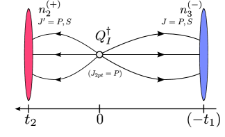
Figure 1: Contractions for the three-point correlation function of the (anti)neutrons with a n¯n¯𝑛𝑛\bar{n}\leftarrow n transition operator. The indices of the neutron interpolating operators refer to the standard Dirac-Pauli representation (see Appendix A).

The three-point functions involve two neutron or two antineutron fields to create and annihilate states with opposite baryon numbers. Using the (anti)neutron states defined in Eq. (98), one can express the three-point correlation function containing, for example, the nn¯𝑛¯𝑛n\leftarrow\bar{n} transition matrix element (see Fig. 1):

GnQIn¯(σ)JJ(t1,t2)=𝐱,𝐲vac|nσ(+)J(𝐱,t2)QI(0)nσ()J(𝐲,t1)|vac=(CΓσ(+))αα𝐱,𝐲nαJ(𝐱,t2)QI(0)nαJ(𝐲,t1).superscriptsubscript𝐺𝑛superscriptsubscript𝑄𝐼¯𝑛𝜎𝐽superscript𝐽subscript𝑡1subscript𝑡2subscript𝐱𝐲quantum-operator-productvacsuperscriptsubscript𝑛𝜎superscript𝐽𝐱subscript𝑡2superscriptsubscript𝑄𝐼0superscriptsubscript𝑛𝜎𝐽𝐲subscript𝑡1vacsubscript𝐶superscriptΓ𝜎𝛼superscript𝛼subscript𝐱𝐲delimited-⟨⟩superscriptsubscript𝑛superscript𝛼superscript𝐽𝐱subscript𝑡2superscriptsubscript𝑄𝐼0superscriptsubscript𝑛𝛼𝐽𝐲subscript𝑡1\begin{split}G_{nQ_{I}^{\dagger}\bar{n}(\sigma)}^{JJ^{\prime}}(t_{1},t_{2})&=\sum_{\mathbf{x},\mathbf{y}}\left<\text{vac}\right|n_{\sigma}^{(+)J^{\prime}}(\mathbf{x},t_{2})Q_{I}^{\dagger}(0)n_{-\sigma}^{(-)J}(\mathbf{y},-t_{1})\left|\text{vac}\right>\\ &=\big{(}C\Gamma^{\sigma(+)}\big{)}_{\alpha\alpha^{\prime}}\sum_{\mathbf{x},\mathbf{y}}\left<n_{\alpha^{\prime}}^{J^{\prime}}(\mathbf{x},t_{2})Q_{I}^{\dagger}(0)n_{\alpha}^{J}(\mathbf{y},-t_{1})\right>.\end{split} (50)

where nσ()subscriptsuperscript𝑛𝜎n^{(-)}_{-\sigma} is nucleon interpolating field that creates an antineutron with spin σ𝜎\sigma555 Note that spin-flip of a spinor incorporates nontrivial signs in order to satisfy n(σ)=nσsubscript𝑛𝜎subscript𝑛𝜎n_{-(-\sigma)}=-n_{\sigma} similar to 𝒯𝒯{\mathcal{T}} transformation, which is responsible for the relative signs of the neutron and antineutron states. , both the (anti)neutron operators are summed over the spatial coordinate to project on zero momentum. By calculating quark propagators with point sources located at the operator insertion point and momentum-projected P𝑃P and S𝑆S sinks located on all time slices, the correlation functions GnQIn¯JJsuperscriptsubscript𝐺𝑛superscriptsubscript𝑄𝐼¯𝑛𝐽superscript𝐽G_{nQ_{I}^{\dagger}\bar{n}}^{JJ^{\prime}} can be accessed for all smearing combinations PP𝑃𝑃PP, PS𝑃𝑆PS, SP𝑆𝑃SP, and SS𝑆𝑆SS, any temporal separation between the source and the sink tsep=t1+t2subscript𝑡sepsubscript𝑡1subscript𝑡2t_{\text{sep}}=t_{1}+t_{2}, and any operator separation from the source τ=t1𝜏subscript𝑡1\tau=t_{1}. The same propagators are used to calculate PP𝑃𝑃PP and PS𝑃𝑆PS two-point correlation functions. The spectral representation for Eq. (50) analogous to Eq. (49) is given by

GnQIn¯(σ)JJ(t1,t2)=m,mZmJZmJeEmt2Emt1(I)mm,superscriptsubscript𝐺𝑛superscriptsubscript𝑄𝐼¯𝑛𝜎𝐽superscript𝐽subscript𝑡1subscript𝑡2subscript𝑚superscript𝑚superscriptsubscript𝑍𝑚𝐽superscriptsubscript𝑍superscript𝑚superscript𝐽superscript𝑒subscript𝐸superscript𝑚subscript𝑡2subscript𝐸𝑚subscript𝑡1subscriptsubscript𝐼𝑚superscript𝑚\begin{split}G_{nQ_{I}^{\dagger}\bar{n}(\sigma)}^{JJ^{\prime}}(t_{1},t_{2})&=\sum_{m,m^{\prime}}\sqrt{Z_{m}^{J}Z_{m^{\prime}}^{J^{\prime}}}e^{-E_{m^{\prime}}t_{2}-E_{m}t_{1}}(\mathcal{M}_{I})_{mm^{\prime}},\end{split} (51)

where (I)mm=m|QI|msubscriptsubscript𝐼superscript𝑚𝑚quantum-operator-productsuperscript𝑚subscript𝑄𝐼𝑚(\mathcal{M}_{I})_{m^{\prime}m}=\left<m^{\prime}\vphantom{Q_{I}m}\right|Q_{I}\left|m\vphantom{m^{\prime}Q_{I}}\right>, the ground-state matrix element of interest is I=(I)00subscript𝐼subscriptsubscript𝐼00\mathcal{M}_{I}=(\mathcal{M}_{I})_{00}, and the overlap factors ZmJsuperscriptsubscript𝑍𝑚𝐽Z_{m}^{J}, ZmJsuperscriptsubscript𝑍superscript𝑚superscript𝐽Z_{m^{\prime}}^{J^{\prime}} are the same as in Eq. 49. We perform contractions for all combinations of point and smeared sources and sinks in the three-point functions to enhance the analysis of the ground and excited state matrix elements in the next section. To reduce stochastic uncertainties, we also average lattice matrix elements over the spins of the neutron and antineutron states. The specific combinations of (anti)neutron 4-spinor components in the three-point functions that give matrix elements Isubscript𝐼{\mathcal{M}}_{I} are

n¯+1/2()|QI|n+1/2(+)quantum-operator-productsubscriptsuperscript¯𝑛12subscript𝑄𝐼subscriptsuperscript𝑛12\displaystyle\left<{\bar{n}^{(-)}_{+1/2}}\vphantom{Q_{I}{n^{(+)}_{+1/2}}}\right|Q_{I}\left|{n^{(+)}_{+1/2}}\vphantom{{\bar{n}^{(-)}_{+1/2}}Q_{I}}\right> n4(t2)QI(0)n1(t1)similar-toabsentdelimited-⟨⟩superscriptsubscript𝑛4subscript𝑡2subscript𝑄𝐼0superscriptsubscript𝑛1subscript𝑡1\displaystyle\sim-\langle n_{4}^{\dagger}(t_{2})Q_{I}(0)n_{1}^{\dagger}(-t_{1})\rangle (52)
n¯1/2()|QI|n1/2(+)quantum-operator-productsubscriptsuperscript¯𝑛12subscript𝑄𝐼subscriptsuperscript𝑛12\displaystyle\left<{\bar{n}^{(-)}_{-1/2}}\vphantom{Q_{I}{n^{(+)}_{-1/2}}}\right|Q_{I}\left|{n^{(+)}_{-1/2}}\vphantom{{\bar{n}^{(-)}_{-1/2}}Q_{I}}\right> n3(t2)QI(0)n2(t1)similar-toabsentdelimited-⟨⟩superscriptsubscript𝑛3subscript𝑡2subscript𝑄𝐼0superscriptsubscript𝑛2subscript𝑡1\displaystyle\sim\phantom{+}\langle n_{3}^{\dagger}(t_{2})Q_{I}(0)n_{2}^{\dagger}(-t_{1})\rangle
n+1/2(+)|QI|n¯+1/2()quantum-operator-productsubscriptsuperscript𝑛12superscriptsubscript𝑄𝐼subscriptsuperscript¯𝑛12\displaystyle\left<{n^{(+)}_{+1/2}}\vphantom{Q_{I}^{\dagger}{\bar{n}^{(-)}_{+1/2}}}\right|Q_{I}^{\dagger}\left|{\bar{n}^{(-)}_{+1/2}}\vphantom{{n^{(+)}_{+1/2}}Q_{I}^{\dagger}}\right> n1(t2)QI(0)n4(t1)similar-toabsentdelimited-⟨⟩subscript𝑛1subscript𝑡2superscriptsubscript𝑄𝐼0subscript𝑛4subscript𝑡1\displaystyle\sim-\langle n_{1}(t_{2})Q_{I}^{\dagger}(0)n_{4}(-t_{1})\rangle
n1/2(+)|QI|n¯1/2()quantum-operator-productsubscriptsuperscript𝑛12superscriptsubscript𝑄𝐼subscriptsuperscript¯𝑛12\displaystyle\left<{n^{(+)}_{-1/2}}\vphantom{Q_{I}^{\dagger}{\bar{n}^{(-)}_{-1/2}}}\right|Q_{I}^{\dagger}\left|{\bar{n}^{(-)}_{-1/2}}\vphantom{{n^{(+)}_{-1/2}}Q_{I}^{\dagger}}\right> n2(t2)QI(0)n3(t1)similar-toabsentdelimited-⟨⟩subscript𝑛2subscript𝑡2superscriptsubscript𝑄𝐼0subscript𝑛3subscript𝑡1\displaystyle\sim\phantom{+}\langle n_{2}(t_{2})Q_{I}^{\dagger}(0)n_{3}(-t_{1})\rangle

where the signs correspond to the conventions listed in Appendix A. As shown in Sec. II.4, these matrix elements are real, and combining them with the conjugated ones is also used to enhance statistics following Eq. (43).

IV Analysis of matrix elements
Refer to caption
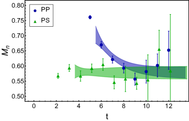
Figure 2: Combined correlated χ2superscript𝜒2\chi^{2} fits of PP𝑃𝑃PP, PS𝑃𝑆PS two-point to Eq. (54) in the time range shown in the first row of Tab. 2. The covariance matrix is estimated with optimal shrinkage λsuperscript𝜆\lambda^{*} as described in the main text. Corresponding data points show the effective masses Mn(t)=lnGnn(t)lnGnn(t+1)subscript𝑀𝑛𝑡subscript𝐺𝑛𝑛𝑡subscript𝐺𝑛𝑛𝑡1M_{n}(t)=\ln G_{nn}(t)-\ln G_{nn}(t+1) with their statistical uncertainties. Note that tmaxsuperscript𝑡𝑚𝑎𝑥t^{max} in Tab. 2 indicates the largest separation for Gnnsubscript𝐺𝑛𝑛G_{nn} considered and that the effective mass is consequently shown for 0ttmax10𝑡superscript𝑡𝑚𝑎𝑥10\leq t\leq t^{max}-1.
tPPminsubscriptsuperscript𝑡𝑚𝑖𝑛𝑃𝑃t^{min}_{PP} tPSminsubscriptsuperscript𝑡𝑚𝑖𝑛𝑃𝑆t^{min}_{PS} tmaxsuperscript𝑡𝑚𝑎𝑥t^{max} Ndofsubscript𝑁dofN_{\text{dof}} E0subscript𝐸0E_{0} E1subscript𝐸1E_{1} χ2/Ndofsuperscript𝜒2subscript𝑁dof\chi^{2}/N_{\text{dof}} λsuperscript𝜆\lambda^{*}
6 4 13 12 0.578(23) 1.23(27) 0.50 0.14
6 6 13 10 0.556(22) 1.11(15) 0.42 0.15
6 5 13 11 0.560(24) 1.13(21) 0.40 0.14
5 5 13 12 0.566(20) 1.26(9) 0.40 0.13
7 5 13 13 0.554(69) 0.98(43) 0.42 0.15
Weighted Ave 0.565(24)(8) 1.21(15)(65)
Table 2: Results of two-point function fits from different time ranges: ground- and excited-state energies, reduced χ2/Ndofsuperscript𝜒2subscript𝑁dof\chi^{2}/N_{\text{dof}}, and optimal shrinkage parameters λsuperscript𝜆\lambda^{*}. The uncertainties in individual fits are statistical. The last line shows “fit averages” with statistical and systematic uncertainties computed as described in Appendix B.3.

To account for excited-state contributions, we perform two-state fits to a truncation of Eq. (50),

GnQIn¯JJ(tsep,τ)=Z0JZ0JeE0tsepI+eE0τE1(tsepτ)𝒜IJJ+eE1τE0(tsepτ)𝒜IJJ+eE1tsepIJJ,superscriptsubscript𝐺𝑛superscriptsubscript𝑄𝐼¯𝑛𝐽superscript𝐽subscript𝑡sep𝜏superscriptsubscript𝑍0𝐽superscriptsubscript𝑍0superscript𝐽superscript𝑒subscript𝐸0subscript𝑡sepsubscript𝐼superscript𝑒subscript𝐸0𝜏subscript𝐸1subscript𝑡sep𝜏superscriptsubscript𝒜𝐼𝐽superscript𝐽superscript𝑒subscript𝐸1𝜏subscript𝐸0subscript𝑡sep𝜏superscriptsubscript𝒜𝐼superscript𝐽𝐽superscript𝑒subscript𝐸1subscript𝑡sepsuperscriptsubscript𝐼𝐽superscript𝐽G_{nQ_{I}^{\dagger}\bar{n}}^{JJ^{\prime}}(t_{\text{sep}},\tau)=\sqrt{Z_{0}^{J}Z_{0}^{J^{\prime}}}e^{-E_{0}t_{\text{sep}}}{\mathcal{M}}_{I}+e^{-E_{0}\tau-E_{1}(t_{\text{sep}}-\tau)}\mathcal{A}_{I}^{JJ^{\prime}}+e^{-E_{1}\tau-E_{0}(t_{\text{sep}}-\tau)}\mathcal{A}_{I}^{J^{\prime}J}+e^{-E_{1}t_{\text{sep}}}\mathcal{B}_{I}^{JJ^{\prime}}\,, (53)

where 𝒜IJJsuperscriptsubscript𝒜𝐼𝐽superscript𝐽\mathcal{A}_{I}^{JJ^{\prime}} and IJJsuperscriptsubscript𝐼𝐽superscript𝐽\mathcal{B}_{I}^{JJ^{\prime}} are products of overlap factors and matrix elements involving only excited states, which are discarded in our calculation. The ground-state overlap factors Z0Psuperscriptsubscript𝑍0𝑃Z_{0}^{P} and Z0Ssuperscriptsubscript𝑍0𝑆Z_{0}^{S} required to extract matrix elements of GnQIn¯JJsuperscriptsubscript𝐺𝑛superscriptsubscript𝑄𝐼¯𝑛𝐽superscript𝐽G_{nQ_{I}^{\dagger}\bar{n}}^{JJ^{\prime}} can be obtained independently from fits of two-point functions GnnPPsuperscriptsubscript𝐺𝑛𝑛𝑃𝑃G_{nn}^{PP} and GnnPSsuperscriptsubscript𝐺𝑛𝑛𝑃𝑆G_{nn}^{PS} to an analogous two-state model

Gnn(σ)JJ(t)=Z0JZ0JeE0t+Z1JZ1JeE1t,superscriptsubscript𝐺𝑛𝑛𝜎𝐽superscript𝐽𝑡superscriptsubscript𝑍0𝐽superscriptsubscript𝑍0superscript𝐽superscript𝑒subscript𝐸0𝑡superscriptsubscript𝑍1𝐽superscriptsubscript𝑍1superscript𝐽superscript𝑒subscript𝐸1𝑡\begin{split}G_{nn(\sigma)}^{JJ^{\prime}}(t)&=\sqrt{Z_{0}^{J}Z_{0}^{J^{\prime}}}e^{-E_{0}t}+\sqrt{Z_{1}^{J}Z_{1}^{J^{\prime}}}e^{-E_{1}t},\end{split} (54)

The energies E0subscript𝐸0E_{0} and E1subscript𝐸1E_{1} appear in both Eq. (53) and Eq. (54), therefore fits of GnQIn¯subscript𝐺𝑛superscriptsubscript𝑄𝐼¯𝑛G_{nQ_{I}^{\dagger}\bar{n}} may be simplified by fixing the state energies E0subscript𝐸0E_{0}, E1subscript𝐸1E_{1} to values determined from fits of two-point functions GnnJJsuperscriptsubscript𝐺𝑛𝑛𝐽superscript𝐽G_{nn}^{JJ^{\prime}}. In principle, the overlaps with excited neutron states Z1Jsuperscriptsubscript𝑍1𝐽Z_{1}^{J} are also determined from two-point function fits, thus the number of parameters in Eq. (53) can be reduced by factoring 𝒜IJJsuperscriptsubscript𝒜𝐼𝐽superscript𝐽\mathcal{A}_{I}^{JJ^{\prime}}, IJJsuperscriptsubscript𝐼𝐽superscript𝐽\mathcal{B}_{I}^{JJ^{\prime}} into excited-state matrix elements and overlap factors Z0,1Jsuperscriptsubscript𝑍01𝐽Z_{0,1}^{J}, of which only the latter would depend on the neutron interpolating operators. It would be possible if the two- and three-point functions were saturated by contributions only from the ground and the first excited states, or their contributions could be reliably distinguished from higher-energy states omitted from Eqs. (53,54). However, as our two-point function fits in Fig. 2 show, there are higher excited-state contributions to Gnnsubscript𝐺𝑛𝑛G_{nn}; in particular, there is large systematic uncertainty on E1subscript𝐸1E_{1} in (see Tab. 2).

These considerations lead us to adopt the following fit strategy: first, a combined fit of GnnPPsuperscriptsubscript𝐺𝑛𝑛𝑃𝑃G_{nn}^{PP} and GnnPSsuperscriptsubscript𝐺𝑛𝑛𝑃𝑆G_{nn}^{PS} to Eq. (54) is used to determine the four parameters E0,1subscript𝐸01E_{0,1} and Z0P,Ssuperscriptsubscript𝑍0𝑃𝑆Z_{0}^{P,S} as summarized in Fig. 2 and Tab. 2; then, a combined fit of GnQIn¯PSsuperscriptsubscript𝐺𝑛superscriptsubscript𝑄𝐼¯𝑛𝑃𝑆G_{nQ_{I}^{\dagger}\bar{n}}^{PS}, GnQIn¯SPsuperscriptsubscript𝐺𝑛superscriptsubscript𝑄𝐼¯𝑛𝑆𝑃G_{nQ_{I}^{\dagger}\bar{n}}^{SP}, and GnQIn¯SSsuperscriptsubscript𝐺𝑛superscriptsubscript𝑄𝐼¯𝑛𝑆𝑆G_{nQ_{I}^{\dagger}\bar{n}}^{SS} to Eq. (53) is used to determine the six parameters Isubscript𝐼{\mathcal{M}}_{I}, 𝒜IPSsuperscriptsubscript𝒜𝐼𝑃𝑆\mathcal{A}_{I}^{PS}, 𝒜ISPsuperscriptsubscript𝒜𝐼𝑆𝑃\mathcal{A}_{I}^{SP}, 𝒜ISSsuperscriptsubscript𝒜𝐼𝑆𝑆\mathcal{A}_{I}^{SS}, IPS=ISPsuperscriptsubscript𝐼𝑃𝑆superscriptsubscript𝐼𝑆𝑃\mathcal{B}_{I}^{PS}=\mathcal{B}_{I}^{SP}, and ISSsuperscriptsubscript𝐼𝑆𝑆\mathcal{B}_{I}^{SS}. Also, since PP𝑃𝑃PP three-point functions would have even large excited-state contamination and PP𝑃𝑃PP three-point/two-point ratios are not close to their plateau region for the tsepsubscript𝑡sept_{\text{sep}} used here (not shown), we do not include GnQIn¯PPsuperscriptsubscript𝐺𝑛superscriptsubscript𝑄𝐼¯𝑛𝑃𝑃G_{nQ_{I}^{\dagger}\bar{n}}^{PP} in our analysis.

Refer to caption
Refer to caption
Refer to caption
Refer to caption
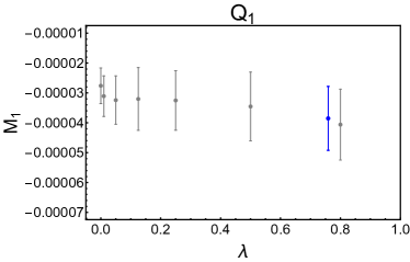
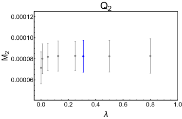
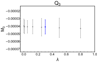
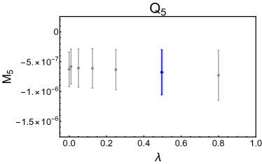
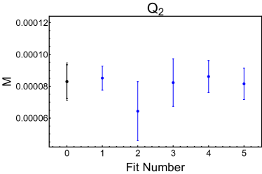
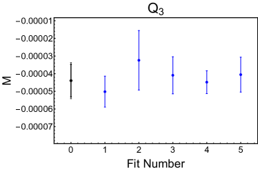
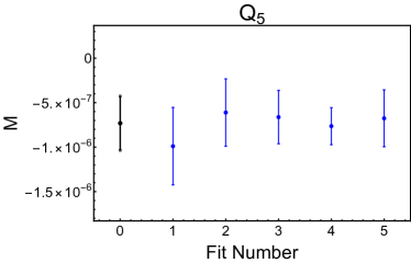
Figure 3: Sensitivity of resulting (bare) matrix elements Isubscript𝐼{\mathcal{M}}_{I} obtained from three-point function fits (Eq. (53)) to the shrinkage parameter λ𝜆\lambda that is used to estimate the covariance matrix as described in the main text (black points). The dark blue points indicate the values obtained with optimal shrinkage parameters λsuperscript𝜆\lambda^{*} (see Eq. (55) and Appendix B.1). The fit ranges are shown in the fourth row of Tab. 3.

With all-mode-averaging described in Sec. III, we obtain one unbiased sample of the two- and three-point functions per gauge field configuration. The number of gauge field configurations used in this calculation Nconf=30subscript𝑁conf30N_{\text{conf}}=30 is not large enough to obtain nondegenerate determination of a covariance matrix for the required number of data points 31K7631𝐾7631\leq K\leq 76 included in the three-point correlator fits. Therefore, spin and parity symmetries are used to increase the effective number of unbiased samples of correlation functions. Thus, GnQn¯subscript𝐺𝑛superscript𝑄¯𝑛G_{nQ^{\dagger}\bar{n}} and Gn(QI𝒫)n¯subscript𝐺𝑛superscriptsuperscriptsubscript𝑄𝐼𝒫¯𝑛G_{n(Q_{I}^{\mathcal{P}})^{\dagger}\bar{n}} with two polarizations are treated as four samples per gauge-field configuration, resulting in N=120𝑁120N=120 samples for each data point after all-mode-averaging bias correction. Polarized two-point functions Gnn(±1/2)subscript𝐺𝑛𝑛plus-or-minus12G_{nn(\pm 1/2)}, Gn¯n¯(±1/2)subscript𝐺¯𝑛¯𝑛plus-or-minus12G_{\bar{n}\bar{n}(\pm 1/2)} are similarly combined to obtain a statistical ensemble of N=120𝑁120N=120 two-point functions. Although this yields an “ensemble” with N>K𝑁𝐾N>K samples, it is still not sufficient for reliable determination of covariance matrix, which typically requires NK2greater-than-or-equivalent-to𝑁superscript𝐾2N\gtrsim K^{2}.

Refer to caption
Refer to caption
Refer to caption
Refer to caption
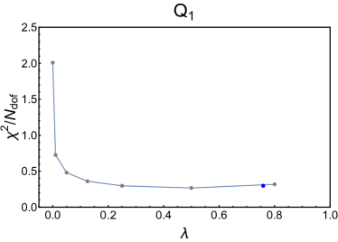
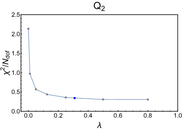
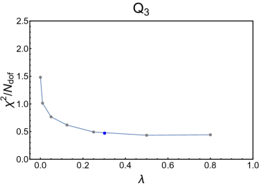
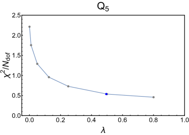
Figure 4: Dependence of correlated χ2/Ndofsuperscript𝜒2subscript𝑁dof\chi^{2}/N_{\text{dof}} values of three-point function fits (Eq. (53)) on the shrinkage parameter λ𝜆\lambda that is used to estimate the covariance matrix as described in the main text (black points). The dark blue points indicate the values obtained with optimal shrinkage parameters λsuperscript𝜆\lambda^{*} (see Eq. (55) and Appendix B.1). The fit ranges are shown in the fourth row of Tab. 3.

For both two-point and three-point functions, finite sample-size fluctuations may make the sample covariance matrix ill-determined and lead to a numerically unstable inverse covariance matrix required for least-squares fitting. Shrinkage Stein (1956); Ledoit and Wolf (2004) has been proposed as a method of improving the condition number of covariance matrix estimates. Denoting the sample covariance matrix by S𝑆S, the corresponding covariance matrix estimate with shrinkage is given by

Σ(λ)=λdiag(S)+(1λ)S,Σ𝜆𝜆diag𝑆1𝜆𝑆\begin{split}\Sigma(\lambda)=\lambda\,\text{diag}(S)+(1-\lambda)S,\end{split} (55)

where 0λ10𝜆10\leq\lambda\leq 1 is the shrinkage parameter, and diag(S)diag𝑆\text{diag}(S) is a particular “shrinkage target”. Taking any λ>0𝜆0\lambda>0 “shrinks” the spectrum of the covariance matrix by reducing the relative size of off-diagonal correlations compared to the diagonal covariance matrix elements. This leads to a better-conditioned covariance matrix and a more robust estimate of the inverse covariance matrix used for χ2superscript𝜒2\chi^{2}-minimization. Trivial λ=0𝜆0\lambda=0 corresponds to no shrinkage, while λ=1𝜆1\lambda=1 removes off-diagonal correlations completely, which is equivalent to an uncorrelated fit. Therefore, varying the parameter 0λ10𝜆10\leq\lambda\leq 1 interpolates continuously between correlated (albeit with potentially poorly-determined covariance matrix) and uncorrelated fits. A standard prescription for choosing the optimal shrinkage parameter is to minimize the rms difference between Σ(λ)Σ𝜆\Sigma(\lambda) and the true covariance matrix. A sample estimator for the optimal shrinkage parameter λsuperscript𝜆\lambda^{*} is suggested in Ref. Ledoit and Wolf (2004) and summarized in Appendix B.1. Bootstrap covariance matrices with optimal shrinkage666 λsuperscript𝜆\lambda^{*} are chosen to provide optimal shrinkage for the normalized sample correlation matrix as described in Appendix B.1 rather than the bootstrap covariance matrix. It is possible that finite-sample-size bias will lead to differences between the optimal shrinkage parameters for the two matrices. Since λsuperscript𝜆\lambda^{*} defined by this prescription vanishes in the infinite-statistics limit, the bootstrap covariance matrix obtained with this choice of shrinkage parameter will provide an unbiased (but not necessarily optimal) estimate of the true covariance matrix in the infinite-statistics limit. Σ=Σ(λ)superscriptΣΣsuperscript𝜆\Sigma^{*}=\Sigma(\lambda^{*}) are obtained by inserting λsuperscript𝜆\lambda^{*} from Eq. (105) into Eq. (55) with S𝑆S the bootstrap covariance matrix obtained from Nboot=10,000subscript𝑁𝑏𝑜𝑜𝑡10000N_{boot}=10,000 samples of two-point and three-point correlation functions. The effects of shrinkage on the central values, uncertainties, and goodness-of-fit of the matrix element fits described below are explored by varying λ𝜆\lambda, and the results for one choice of fit range are shown in Figs. 3-4. For all operators, the central values and the statistical uncertainties are relatively insensitive to the value of the shrinkage parameter once λ>0𝜆0\lambda>0. The χ2/Ndofsuperscript𝜒2subscript𝑁dof\chi^{2}/N_{\text{dof}} values decrease sharply in a small region around λ=0𝜆0\lambda=0, however they are much less sensitive for larger λ𝜆\lambda values. In all cases, the optimal values λsuperscript𝜆\lambda^{*} for the shrinkage parameter are found outside of the region of strong dependence of χ2superscript𝜒2\chi^{2} on λ𝜆\lambda.

Refer to caption
Refer to caption
Refer to caption
Refer to caption
Refer to caption
Refer to caption
Refer to caption
Refer to caption
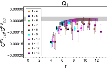
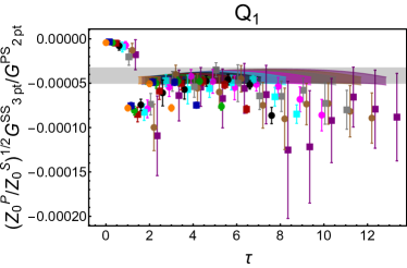
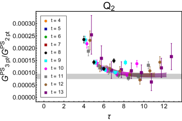
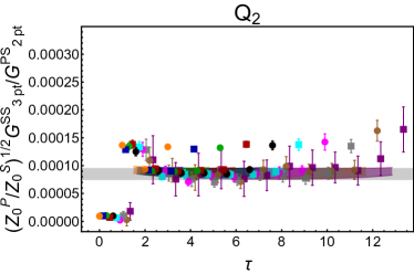
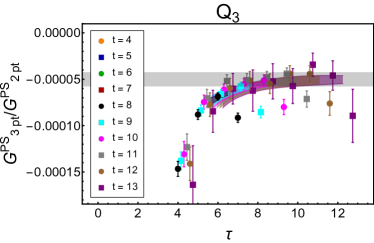
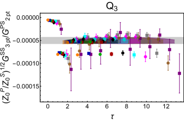
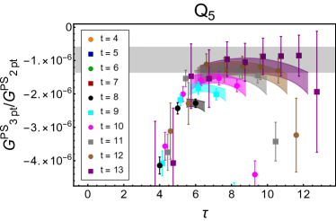
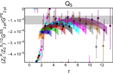
Figure 5: Combined correlated χ2superscript𝜒2\chi^{2} fits of PS𝑃𝑆PS, SS𝑆𝑆SS three-point functions to Eq. (53) for operators Q1subscript𝑄1Q_{1}, Q2subscript𝑄2Q_{2}, Q3subscript𝑄3Q_{3}, and Q5subscript𝑄5Q_{5} for the time range shown in the first row of Tab. 3 (shaded bands). The state energies are determined from fits to two-point functions as shown in Fig. 2. Covariance matrix is estimated with optimal shrinkage λsuperscript𝜆\lambda^{*} as described in the main text. Corresponding data points for ratios of three- to two-point correlation functions for all used source/sink separations tsepsubscript𝑡sept_{\text{sep}} are shown with intermittent square and circle data points. The central values of matrix elements Isubscript𝐼{\mathcal{M}}_{I} and their statistical uncertainties are shown with gray shaded bands. All the displayed uncertainties are statistical and estimated using bootstrap.

The average two-point function and the corresponding bootstrap covariance matrix with optimal shrinkage are used for nonlinear χ2superscript𝜒2\chi^{2}-minimization to determine E0subscript𝐸0E_{0}, E1subscript𝐸1E_{1}, Z0Psuperscriptsubscript𝑍0𝑃\sqrt{Z_{0}^{P}}, and Z0Ssuperscriptsubscript𝑍0𝑆\sqrt{Z_{0}^{S}}. χ2superscript𝜒2\chi^{2}-minimization is reduced to a two-parameter optimization problem by variable projection(VarPro) technique Golub and Pereyra (2003); Dianne P. O’Leary (2013) detailed in Appendix B.2. In VarPro, the products of overlap factors in Eq. (54) are found from a linear χ2superscript𝜒2\chi^{2}-fit for particular values of E0,1subscript𝐸01E_{0,1} and the solution is substituted back into χ2superscript𝜒2\chi^{2} in order to obtain a two-parameter function χVP2(E0,E1)subscriptsuperscript𝜒2𝑉𝑃subscript𝐸0subscript𝐸1\chi^{2}_{VP}(E_{0},E_{1}), which is then minimized using nonlinear numerical methods. With these four parameters held fixed, the remaining six free parameters in the three-point function fit (53) can also be found from a linear χ2superscript𝜒2\chi^{2} fit. The parameter covariance matrix for all 10 parameters is subsequently estimated using an additional correlated bootstrap resampling and fitting of two- and three-point function data. The original bootstrap covariance matrices are used in all these fits in order to avoid the possibility of ill-conditioned covariance matrices. The bootstrap parameter covariance matrix is obtained from Nboot=200superscriptsubscript𝑁𝑏𝑜𝑜𝑡200N_{boot}^{\prime}=200 correlated resampling draws. The parameter covariance matrix is diagonalized, the eigenvalues are resampled Nboot′′=200superscriptsubscript𝑁𝑏𝑜𝑜𝑡′′200N_{boot}^{\prime\prime}=200 times, and the resampled eigenvalues are transformed back to the original parameter basis. Finally, the standard deviation of the resulting resampled values of Isubscript𝐼{\mathcal{M}}_{I} is used to define the marginalized uncertainty of Isubscript𝐼{\mathcal{M}}_{I} for each fit range shown in Tab. 3. An analogous procedure is used to obtain the uncertainties of E0subscript𝐸0E_{0} and E1subscript𝐸1E_{1} shown in Tab. 2. Results for the matrix elements from the fits that include our smallest tsepsubscript𝑡sept_{\text{sep}} value are compared to the ratios of three-point to two-point functions (adjusting for proper overlap factors) in Figs. 5. In addition, the two-point function fits are compared to the corresponding effective masses in Fig. 2.
Refer to caption
Refer to caption
Refer to caption
Refer to caption
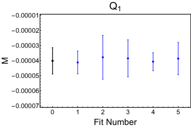
Figure 6: Comparison of ground state matrix elements (lattice units) extracted in fits with different fit ranges that are listed in Tab. 3. The black point at zero indicates the result of the weighted averaging procedure described in Appendix B.3, and the small and large error bars indicate statistical and statistical-plus-systematic uncertainties, respectively.

Systematic uncertainties of our analysis procedure are studied by varying the time ranges of data included in the two-state fits. Results of fits of two-point function data Gnn(n¯n¯)PP(tPPminttsepmax)subscriptsuperscript𝐺𝑃𝑃𝑛𝑛¯𝑛¯𝑛subscriptsuperscript𝑡𝑚𝑖𝑛𝑃𝑃𝑡superscriptsubscript𝑡sep𝑚𝑎𝑥G^{PP}_{nn(\bar{n}\bar{n})}(t^{min}_{PP}\leq t\leq t_{\text{sep}}^{max}) and Gnn(n¯n¯)PS(tPSminttsepmax)subscriptsuperscript𝐺𝑃𝑆𝑛𝑛¯𝑛¯𝑛subscriptsuperscript𝑡𝑚𝑖𝑛𝑃𝑆𝑡superscriptsubscript𝑡sep𝑚𝑎𝑥G^{PS}_{nn(\bar{n}\bar{n})}(t^{min}_{PS}\leq t\leq t_{\text{sep}}^{max}) for a variety of tPPminsubscriptsuperscript𝑡𝑚𝑖𝑛𝑃𝑃t^{min}_{PP} and tPSminsubscriptsuperscript𝑡𝑚𝑖𝑛𝑃𝑆t^{min}_{PS} are shown in Tab. 2. Results of corresponding fits of three-point function data GnQIn¯SS(τminP+τminStseptsepmax,τminSτtsepτminS)G_{nQ_{I}^{\dagger}\bar{n}}^{SS}(\tau_{min}^{P}+\tau_{min}^{S}\leq t_{\text{sep}}\leq t_{\text{sep}}^{max},\tau_{min}^{S}\leq\tau\leq t_{\text{sep}}-\tau_{min}^{S}) and GnQIn¯PS(2τminStseptsepmax,τminPτtsepτminS)G_{nQ_{I}^{\dagger}\bar{n}}^{PS}(2\tau_{min}^{S}\leq t_{\text{sep}}\leq t_{\text{sep}}^{max},\tau_{min}^{P}\leq\tau\leq t_{\text{sep}}-\tau_{min}^{S}) for a variety of τminSsuperscriptsubscript𝜏𝑚𝑖𝑛𝑆\tau_{min}^{S} and τminPsuperscriptsubscript𝜏𝑚𝑖𝑛𝑃\tau_{min}^{P} are shown in Tab. 3. The data for SP𝑆𝑃SP and PS𝑃𝑆PS three-point correlation functions are averaged using relation GnQIn¯SP(tsep,τ)=GnQIn¯PS(tsep,tsepτ)superscriptsubscript𝐺𝑛superscriptsubscript𝑄𝐼¯𝑛𝑆𝑃subscript𝑡sep𝜏superscriptsubscript𝐺𝑛superscriptsubscript𝑄𝐼¯𝑛𝑃𝑆subscript𝑡sepsubscript𝑡sep𝜏G_{nQ_{I}^{\dagger}\bar{n}}^{SP}(t_{\text{sep}},\tau)=G_{nQ_{I}^{\dagger}\bar{n}}^{PS}(t_{\text{sep}},t_{\text{sep}}-\tau) to reduce the number of data points in the fits. Results for bare ground-state matrix elements from different fits are in very good agreement with each other, as shown in Fig.6.

The five fit range choices shown in Tabs. 2-3 result in acceptable correlated χ2/Ndofsuperscript𝜒2subscript𝑁dof\chi^{2}/N_{\text{dof}} values in fits of two- and three-point function data. These results are combined into final estimates of Isubscript𝐼{\mathcal{M}}_{I} and estimates of their statistical and systematic uncertainties. Since the various fits have different Ndofsubscript𝑁dofN_{\text{dof}}, we use a weighted-averaging procedure defined in Appendix B.3. For a particular fit, the weight is a combination of the likelihood that the fit describes the data (we use its p𝑝p-value as the likelihood proxy) and its statistical precision, to penalize both fits that fail to describe data and fits that do not constrain the relevant parameters. The same weights are used to determine the average statistical uncertainty, which ensures that including multiple similar fits will not lead to a spurious reduction in the final statistical uncertainty. The weighted mean-square difference between each fit result and the weighted average is used to define the systematic uncertainty due to arbitrariness of choice of a fit window. Applying this weighted averaging procedure to the ground-state energy E0subscript𝐸0E_{0} of the two-point function yields the result for the nucleon mass that agrees well with the physical value,

E0=0.565(24)(8)a1=977(42)(13) MeV,subscript𝐸00.565248superscript𝑎19774213 MeV\begin{split}E_{0}=0.565(24)(8)a^{-1}=977(42)(13)\text{ MeV},\end{split} (56)

where we have used the scale-setting result a=0.1141(3)fm𝑎0.11413fma=0.1141(3)\,\text{fm} from Ref. Blum et al. (2016), which has negligible uncertainty for our purposes as it is much smaller compared to other uncertainties in our calculation. Applying the same procedure to the fit results in Tab. 3 provides our final estimate of the bare matrix elements including statistical and fitting systematic uncertainties,

1lat=3.99(1.08)(0.13)×105a6=107(29)(3)×105 GeV62lat=8.28(1.29)(0.54)×105a6=221(35)(14)×105 GeV63lat=4.37(0.86)(0.52)×105a6=117(23)(14)×105 GeV65lat=0.075(32)(10)×105a6=2.01(86)(22)×105 GeV6.superscriptsubscript1lat3.991.080.13superscript105superscript𝑎6107293superscript105superscript GeV6superscriptsubscript2lat8.281.290.54superscript105superscript𝑎62213514superscript105superscript GeV6superscriptsubscript3lat4.370.860.52superscript105superscript𝑎61172314superscript105superscript GeV6superscriptsubscript5lat0.0753210superscript105superscript𝑎62.018622superscript105superscript GeV6\begin{split}{\mathcal{M}}_{1}^{\text{lat}}&=-3.99(1.08)(0.13)\times 10^{-5}a^{-6}=-107(29)(3)\times 10^{-5}\text{ GeV}^{6}\\ {\mathcal{M}}_{2}^{\text{lat}}&=8.28(1.29)(0.54)\times 10^{-5}a^{-6}=221(35)(14)\times 10^{-5}\text{ GeV}^{6}\\ {\mathcal{M}}_{3}^{\text{lat}}&=-4.37(0.86)(0.52)\times 10^{-5}a^{-6}=-117(23)(14)\times 10^{-5}\text{ GeV}^{6}\\ {\mathcal{M}}_{5}^{\text{lat}}&=-0.075(32)(10)\times 10^{-5}a^{-6}=-2.01(86)(22)\times 10^{-5}\text{ GeV}^{6}.\end{split} (57)

These lattice regularized matrix elements can be related to renormalized matrix elements through NPR as described in the next section.

τPminsubscriptsuperscript𝜏𝑚𝑖𝑛𝑃\tau^{min}_{P} τSminsubscriptsuperscript𝜏𝑚𝑖𝑛𝑆\tau^{min}_{S} tsepmaxsuperscriptsubscript𝑡sep𝑚𝑎𝑥t_{\text{sep}}^{max} Ndofsubscript𝑁dofN_{\text{dof}} 1lat×105superscriptsubscript1latsuperscript105{\mathcal{M}}_{1}^{\text{lat}}\times 10^{5} χ2/Ndofsuperscript𝜒2subscript𝑁dof\chi^{2}/N_{\text{dof}} λsuperscript𝜆\lambda^{*} 2lat×105superscriptsubscript2latsuperscript105{\mathcal{M}}_{2}^{\text{lat}}\times 10^{5} χ2/Ndofsuperscript𝜒2subscript𝑁dof\chi^{2}/N_{\text{dof}} λsuperscript𝜆\lambda^{*} 3lat×105superscriptsubscript3latsuperscript105{\mathcal{M}}_{3}^{\text{lat}}\times 10^{5} χ2/Ndofsuperscript𝜒2subscript𝑁dof\chi^{2}/N_{\text{dof}} λsuperscript𝜆\lambda^{*} 5lat×105superscriptsubscript5latsuperscript105{\mathcal{M}}_{5}^{\text{lat}}\times 10^{5} χ2/Ndofsuperscript𝜒2subscript𝑁dof\chi^{2}/N_{\text{dof}} λsuperscript𝜆\lambda^{*}
6 2 13 70 -4.13(0.92) 0.25 0.77 8.50(1.07) 0.40 0.35 -5.01(0.76) 0.44 0.32 -0.098(39) 0.62 0.53
6 4 13 25 -3.81(1.78) 0.44 0.72 6.46(2.15) 0.31 0.31 -3.21(1.25) 0.40 0.29 -0.063(45) 0.53 0.41
6 3 13 45 -3.85(1.07) 0.30 0.76 8.24(1.52) 0.34 0.31 -4.09(0.95) 0.47 0.30 -0.068(38) 0.54 0.50
5 3 13 51 -4.09(0.92) 0.28 0.75 8.61(1.06) 0.34 0.29 -4.50(0.67) 0.44 0.29 -0.077(22) 0.54 0.47
7 3 13 40 -3.87(1.13) 0.34 0.76 8.13(1.32) 0.37 0.32 -4.05(1.00) 0.50 0.31 -0.069(32) 0.55 0.53
Weighted Ave -3.99(1.08)(0.13) 8.28(1.29)(0.54) -4.37(0.86)(0.52) -0.075(32)(10)
Table 3: Fit ranges, bare matrix element results and uncertainties in lattice units, reduced χ2superscript𝜒2\chi^{2} showing goodness-of-fit, and optimal shrinkage parameters used for each three-point function fit for the electroweak-singlet operators Q1subscript𝑄1Q_{1}, Q2subscript𝑄2Q_{2}, Q3subscript𝑄3Q_{3}, and Q5subscript𝑄5Q_{5}.

V Renormalization of lattice operators

Since the matrix elements of the 6-quark operators are computed on a lattice, they have to be converted to some perturbative scheme, e.g., MS¯¯MS\overline{\text{MS}}, before they can be used in BSM phenomenology. We calculate conversion factors between lattice-regularized operators and their perturbative definitions nonperturbatively, by computing their Green’s functions on a lattice and matching them to perturbative calculations. The operators QI(𝒫)subscriptsuperscript𝑄𝒫𝐼Q^{({\mathcal{P}})}_{I} are the lowest-dimension operators with ΔB=2Δ𝐵2\Delta B=-2, therefore they can only either mix with each other, or get discretization corrections from higher-dimensional operators that vanish in the continuum limit. In the chiral basis, all the 14 operators transform differently under U(2)LU(2)Rtensor-product𝑈subscript2𝐿𝑈subscript2𝑅U(2)_{L}\otimes U(2)_{R} flavor symmetry, so they can mix only due to the spontaneous chiral symmetry breaking (Sχ𝜒\chiSB) in QCD, non-perturbative U(1)A𝑈subscript1𝐴U(1)_{A} violation, or chiral symmetry violations by quark masses and discretization of the fermion action. Mixing due to quark masses and non-perturbative effects should be small if renormalization is carried out in the UV region |p|μ{ΛQCD,mq}𝑝𝜇much-greater-thansubscriptΛ𝑄𝐶𝐷subscript𝑚𝑞|p|\approx\mu\gg\{\Lambda_{QCD},m_{q}\} where perturbative matching is applicable. Furthermore, effects of the explicit chiral symmetry violation by the (M)DWF fermion action on a lattice are suppressed as the “residual mass” mresmqless-than-or-similar-tosubscript𝑚𝑟𝑒𝑠subscript𝑚𝑞m_{res}\lesssim m_{q} Blum et al. (2016), and thus are also negligible. Therefore, we don’t expect that renormalization of our results will be affected by mixing between the chiral-basis operators 777 This holds even without taking the continuum limit, since the continuum and the chiral limits can be taken separately in calculations with the (M)DWF lattice fermions, see Ref. Blum et al. (2016) and references within. .

V.1 RI-MOM amplitudes on a lattice

The lattice renormalization constants for the 6-quark operators are defined as

QIR(μ)=ZIJlat(μ,a)QJlat(a)superscriptsubscript𝑄𝐼𝑅𝜇superscriptsubscript𝑍𝐼𝐽lat𝜇𝑎superscriptsubscript𝑄𝐽lat𝑎Q_{I}^{R}(\mu)=Z_{IJ}^{\text{lat}}(\mu,a)Q_{J}^{\text{lat}}(a) (58)

but, as will be shown below, in the chiral-diagonal basis |ZIJ|ZIIZImuch-less-thansubscript𝑍𝐼𝐽subscript𝑍𝐼𝐼subscript𝑍𝐼|Z_{I\neq J}|\ll Z_{II}\equiv Z_{I}, so QIR(μ)=ZIQIlatsuperscriptsubscript𝑄𝐼𝑅𝜇subscript𝑍𝐼superscriptsubscript𝑄𝐼latQ_{I}^{R}(\mu)=Z_{I}Q_{I}^{\text{lat}} both on a lattice and in continuum perturbation theory. The nonperturbative renormalization and mixing of the six-quark operators is computed using a variant of the RI-MOM scheme Martinelli et al. (1995) with a specific choice of momenta of the external quark states. Since the external states are not color-singlets, the gauge is fixed to the Landau gauge using the Fourier-accelerated conjugate gradient algorithm Hudspith (2015). All the operators of interest with ΔB=2Δ𝐵2\Delta B=2 and ΔI=1Δ𝐼1\Delta I=1 888 Instead of the 6-quark, we study renormalization of the 6-antiquark operators, which is equivalent but is more natural on a lattice since it does not require conjugating quark propagators. can be represented in the generic form

Q¯Isubscript¯𝑄𝐼\displaystyle\overline{Q}_{I} =(ΓI)α1α2α3α4α5α6a1a2a3a4a5a6d¯α6a6d¯α5a5d¯α4a4d¯α3a3u¯α2a2u¯α1a1absentsubscriptsuperscriptsubscriptΓ𝐼subscript𝑎1subscript𝑎2subscript𝑎3subscript𝑎4subscript𝑎5subscript𝑎6subscript𝛼1subscript𝛼2subscript𝛼3subscript𝛼4subscript𝛼5subscript𝛼6subscriptsuperscript¯𝑑subscript𝑎6subscript𝛼6subscriptsuperscript¯𝑑subscript𝑎5subscript𝛼5subscriptsuperscript¯𝑑subscript𝑎4subscript𝛼4subscriptsuperscript¯𝑑subscript𝑎3subscript𝛼3subscriptsuperscript¯𝑢subscript𝑎2subscript𝛼2subscriptsuperscript¯𝑢subscript𝑎1subscript𝛼1\displaystyle=(\Gamma_{I})^{a_{1}a_{2}a_{3}a_{4}a_{5}a_{6}}_{\alpha_{1}\alpha_{2}\alpha_{3}\alpha_{4}\alpha_{5}\alpha_{6}}\bar{d}^{a_{6}}_{\alpha_{6}}\bar{d}^{a_{5}}_{\alpha_{5}}\bar{d}^{a_{4}}_{\alpha_{4}}\bar{d}^{a_{3}}_{\alpha_{3}}\bar{u}^{a_{2}}_{\alpha_{2}}\bar{u}^{a_{1}}_{\alpha_{1}} (59)
=(ΓI)[A1A2][A3A6]d¯[A6d¯A5d¯A4d¯A3]u¯[A2u¯A1],\displaystyle=(\Gamma_{I})^{[A_{1}A_{2}][A_{3}\ldots A_{6}]}\bar{d}^{[A_{6}}\bar{d}^{A_{5}}\bar{d}^{A_{4}}\bar{d}^{A_{3}]}\bar{u}^{[A_{2}}\bar{u}^{A_{1}]}\,,

where Ai=(αi,ai)subscript𝐴𝑖subscript𝛼𝑖subscript𝑎𝑖A_{i}=(\alpha_{i},a_{i}) are the spin×\timescolor indices. Then their Green’s functions with external plane-wave quark states,

GIB1B6({pi})=xieiipixiQ¯I(0)uB1(x1)dB6(x6).superscriptsubscript𝐺𝐼subscript𝐵1subscript𝐵6subscript𝑝𝑖subscriptsubscript𝑥𝑖superscript𝑒𝑖subscript𝑖subscript𝑝𝑖subscript𝑥𝑖delimited-⟨⟩subscript¯𝑄𝐼0superscript𝑢subscript𝐵1subscript𝑥1superscript𝑑subscript𝐵6subscript𝑥6G_{I}^{B_{1}\ldots B_{6}}(\{p_{i}\})=\sum_{x_{i}}\,e^{i\sum_{i}p_{i}x_{i}}\,\langle\overline{Q}_{I}(0)u^{B_{1}}(x_{1})\dotsb d^{B_{6}}(x_{6})\rangle\,. (60)

are computed on a lattice contracting six quark propagators computed with a point source at the operator location. The same propagators are used as for the n-n¯𝑛-¯𝑛n\text{-}\overline{n} three-point correlators (see Sec. III), with the only difference that prior to the contraction the propagators are Fourier-transformed at the sink. The six-quark vertex functions are obtained by “amputating” the Green’s functions (60)

ΛIA1A6({pi})superscriptsubscriptΛ𝐼subscript𝐴1subscript𝐴6subscript𝑝𝑖\displaystyle\Lambda_{I}^{A_{1}\ldots A_{6}}(\{p_{i}\}) =Q¯I(0)uA1(p1)dA6(p6)ampabsentsubscriptdelimited-⟨⟩subscript¯𝑄𝐼0superscript𝑢subscript𝐴1subscript𝑝1superscript𝑑subscript𝐴6subscript𝑝6amp\displaystyle=\langle\overline{Q}_{I}(0)u^{A_{1}}(p_{1})\dotsb d^{A_{6}}(p_{6})\rangle_{\text{amp}} (61)
=GIB1B6({pi})[S1(p1)]B1A1[S1(p6)]B6A6,absentsuperscriptsubscript𝐺𝐼subscript𝐵1subscript𝐵6subscript𝑝𝑖superscriptdelimited-[]superscript𝑆1subscript𝑝1subscript𝐵1subscript𝐴1superscriptdelimited-[]superscript𝑆1subscript𝑝6subscript𝐵6subscript𝐴6\displaystyle=G_{I}^{B_{1}\ldots B_{6}}(\{p_{i}\})\cdot[S^{-1}(p_{1})]^{B_{1}A_{1}}\dotsm[S^{-1}(p_{6})]^{B_{6}A_{6}}\,,

where contraction in {Bi}subscript𝐵𝑖\{B_{i}\} is implied, and the momentum-projected quark propagators are

SAB(p)=xeipxqA(x)q¯B(0)superscript𝑆𝐴𝐵𝑝subscript𝑥superscript𝑒𝑖𝑝𝑥delimited-⟨⟩superscript𝑞𝐴𝑥superscript¯𝑞𝐵0S^{AB}(p)=\sum_{x}\,e^{ipx}\,\langle q^{A}(x)\bar{q}^{B}(0)\rangle (62)

Note that the amputated Green’s functions (61) are not symmetric with respect to permutation of the spin×\timescolor indices Aisubscript𝐴𝑖A_{i}, unlike the tree-level vertex function Γi[A1A2][A3A6]superscriptsubscriptΓ𝑖delimited-[]subscript𝐴1subscript𝐴2delimited-[]subscript𝐴3subscript𝐴6\Gamma_{i}^{[A_{1}A_{2}][A_{3}\ldots A_{6}]} in Eq. (59). This is due to the fact that GI({pi})subscript𝐺𝐼subscript𝑝𝑖G_{I}(\{p_{i}\}) and ΛI({pi})subscriptΛ𝐼subscript𝑝𝑖\Lambda_{I}(\{p_{i}\}) depend on the non-equal momenta pisubscript𝑝𝑖p_{i} of the external fields. Such dependency would break the isospin symmetry and thus may mix operators from different chiral representations.

Refer to caption
Figure 7: Momentum configuration for nonperturbative renormalization of 6-quark operators using RI-MOM scheme (only one permutation).

One must choose specific momenta for external quark fields in order to preserve the chiral isospin symmetry. The simplest choice pi=psubscript𝑝𝑖𝑝p_{i}=p would result in a large momentum p𝒪=6psubscript𝑝𝒪6𝑝p_{\mathcal{O}}=6p at the operator insertion leading to large perturbative corrections in conversion to the MS¯¯MS\overline{\text{MS}} scheme. To avoid that, the external quark momenta are arranged so that ipi=0subscript𝑖subscript𝑝𝑖0\sum_{i}p_{i}=0 and, specifically, pi=±psubscript𝑝𝑖plus-or-minus𝑝p_{i}=\pm p (see Fig. 7), where p2=μ2superscript𝑝2superscript𝜇2p^{2}=\mu^{2} determines the scale for perturbative RI-MOM MS¯absent¯MS\to\,\overline{\text{MS}} matching. In addition, the amputated amplitudes (61) must be averaged over permutations of the ±pplus-or-minus𝑝\pm p momenta to enforce the symmetry with respect to the external quark states Syritsyn et al. (2016),

ΛI[A1A2][A3A6](p)=[\displaystyle\Lambda_{I}^{[A_{1}A_{2}][A_{3}\ldots A_{6}]}(p)=\Big{[} 15Q¯Iu(+p)u(+p)d(+p)d(p)d(p)d(p)amp15subscriptdelimited-⟨⟩subscript¯𝑄𝐼𝑢𝑝𝑢𝑝𝑑𝑝𝑑𝑝𝑑𝑝𝑑𝑝amp\displaystyle\frac{1}{5}\langle\overline{Q}_{I}\,u(+p)u(+p)d(+p)d(-p)d(-p)d(-p)\rangle_{\text{amp}} (63)
+\displaystyle+ 35Q¯Iu(+p)u(p)d(+p)d(+p)d(p)d(p)amp35subscriptdelimited-⟨⟩subscript¯𝑄𝐼𝑢𝑝𝑢𝑝𝑑𝑝𝑑𝑝𝑑𝑝𝑑𝑝amp\displaystyle\frac{3}{5}\langle\overline{Q}_{I}\,u(+p)u(-p)d(+p)d(+p)d(-p)d(-p)\rangle_{\text{amp}}
+\displaystyle+ 15Q¯Iu(p)u(p)d(+p)d(+p)d(+p)d(p)amp][A1A2][A3A6],\displaystyle\frac{1}{5}\langle\overline{Q}_{I}\,u(-p)u(-p)d(+p)d(+p)d(+p)d(-p)\rangle_{\text{amp}}\Big{]}^{[A_{1}A_{2}][A_{3}\ldots A_{6}]}\,,

where the factors are determined by combinatorics. All possible permutations of momenta are implicitly included by Wick contractions, and the symmetries of the color×\timesspin indices are restored automatically. Perturbative matching at the one-loop level for this particular scheme has been computed in Ref. Buchoff and Wagman (2016).

The lattice renormalization factors Zlat(p2)superscript𝑍latsuperscript𝑝2Z^{\text{lat}}(p^{2}) (58) can be computed by imposing the condition

Zq3(p)ZIJlat(p)ΛJ{Ai}(p)=ΓI{Ai},superscriptsubscript𝑍𝑞3𝑝subscriptsuperscript𝑍lat𝐼𝐽𝑝superscriptsubscriptΛ𝐽subscript𝐴𝑖𝑝superscriptsubscriptΓ𝐼subscript𝐴𝑖Z_{q}^{-3}(p)Z^{\text{lat}}_{IJ}(p)\,\Lambda_{J}^{\{A_{i}\}}(p)=\Gamma_{I}^{\{A_{i}\}}\,, (64)

where Zqsubscript𝑍𝑞Z_{q} is the lattice quark field renormalization factor

qR(μ)=Zq1/2(μ,a)qlat.superscript𝑞𝑅𝜇superscriptsubscript𝑍𝑞12𝜇𝑎superscript𝑞latq^{R}(\mu)=Z_{q}^{1/2}(\mu,a)q^{\text{lat}}\,. (65)

The renormalization factors ZIJlatsuperscriptsubscript𝑍𝐼𝐽latZ_{IJ}^{\text{lat}} can be expressed in terms of the amputated and symmetrized vertex functions ΛI{Ai}(p)superscriptsubscriptΛ𝐼subscript𝐴𝑖𝑝\Lambda_{I}^{\{A_{i}\}}(p) that are projected onto the original tree-level structures ΓJ{Ai}superscriptsubscriptΓ𝐽subscript𝐴𝑖\Gamma_{J}^{\{A_{i}\}},

ZIJlat(p)subscriptsuperscript𝑍lat𝐼𝐽𝑝\displaystyle Z^{\text{lat}}_{IJ}(p) =Zq3(p)[Λ1(p)]IJ,absentsuperscriptsubscript𝑍𝑞3𝑝subscriptdelimited-[]superscriptΛ1𝑝𝐼𝐽\displaystyle=Z_{q}^{3}(p)\big{[}\Lambda^{-1}(p)]_{IJ}\,, (66)
ΛIJ(p)subscriptΛ𝐼𝐽𝑝\displaystyle\Lambda_{IJ}(p) =[AiΛI{Ai}ΓK{Ai}](g1)KJ,absentdelimited-[]subscriptsubscript𝐴𝑖superscriptsubscriptΛ𝐼subscript𝐴𝑖superscriptsubscriptΓ𝐾absentsubscript𝐴𝑖subscriptsuperscript𝑔1𝐾𝐽\displaystyle=\big{[}\sum_{A_{i}}\Lambda_{I}^{\{A_{i}\}}\Gamma_{K}^{*\{A_{i}\}}\big{]}(g^{-1})_{KJ}\,, (67)
gJKsubscript𝑔𝐽𝐾\displaystyle g_{JK} =AiΓJ{Ai}ΓK{Ai},absentsubscriptsubscript𝐴𝑖superscriptsubscriptΓ𝐽subscript𝐴𝑖superscriptsubscriptΓ𝐾absentsubscript𝐴𝑖\displaystyle=\sum_{A_{i}}\Gamma_{J}^{\{A_{i}\}}\Gamma_{K}^{*\{A_{i}\}}\,, (68)

where the “metric tensor” gJKsubscript𝑔𝐽𝐾g_{JK} is diagonal in the chiral basis Q¯I(𝒫)superscriptsubscript¯𝑄𝐼𝒫\overline{Q}_{I}^{({\mathcal{P}})}. (Approximate) chiral symmetry on a lattice is important for ensuring that ZIJsuperscript𝑍𝐼𝐽Z^{IJ} and ΛIJsubscriptΛ𝐼𝐽\Lambda_{IJ} are also (predominantly) diagonal in this basis. Deviations from the diagonal form are due to the nonzero quark mass and residual chiral symmetry breaking of the DWF discretization. The effect of symmetrization (63) is evident from the magnitude of the off-diagonal components, which is shown in the log scale as the matrix

XIJ=log(|ΛIJ|ΛIIΛJJ)subscript𝑋𝐼𝐽subscriptΛ𝐼𝐽subscriptΛ𝐼𝐼subscriptΛ𝐽𝐽X_{IJ}=\log\Big{(}\frac{|\Lambda_{IJ}|}{\sqrt{\Lambda_{II}\Lambda_{JJ}}}\Big{)} (69)

in Fig. 8 comparing the momentum permutation-averaged amplitude (63) to the one with a specific choice of momentum p1=p3=p4=p2=p4=p6=psubscript𝑝1subscript𝑝3subscript𝑝4subscript𝑝2subscript𝑝4subscript𝑝6𝑝p_{1}=p_{3}=p_{4}=-p_{2}=-p_{4}=-p_{6}=p as in Fig. 7. These data are shown for the momentum p=2πa(1148,1148,1148,22.596)𝑝2𝜋𝑎11481148114822.596p=\frac{2\pi}{a}\big{(}\frac{11}{48},\frac{11}{48},\frac{11}{48},\frac{22.5}{96}\big{)}, which is close to a 4d diagonal direction (up to (π/L)𝜋𝐿(\pi/L) along the time axis due to the antiperiodic boundary conditions) and p2(5GeV)2superscript𝑝2superscript5GeV2p^{2}\approx(5\,\text{GeV})^{2}. Therefore, we conclude that in the chiral basis the renormalization matrix ZIJsubscript𝑍𝐼𝐽Z_{IJ} is diagonal, |ZIJ|/ZIIZIJO(103)less-than-or-similar-tosubscript𝑍𝐼𝐽subscript𝑍𝐼𝐼subscript𝑍𝐼𝐽𝑂superscript103|Z_{IJ}|/\sqrt{Z_{II}Z_{IJ}}\lesssim O(10^{-3}), which is definitely within our target precision, and the operators QI(P)subscriptsuperscript𝑄𝑃𝐼Q^{(P)}_{I} may be renormalized multiplicatively in our lattice calculation. Additionally, we observe that the mixing between 6-quark operators containing different numbers of L,R𝐿𝑅L,R-diquarks is negligible, indicating that nonperturbative chirality-changing effects due to fluctuations of topology of the QCD vacuum do not lead to mixing in excess of the 103superscript10310^{-3} level.

Refer to caption
Refer to caption
Figure 8: Magnitude of the off-diagonal components of the lattice mixing matrix  (69) for (approximately) 4d-diagonal momentum p2=(5GeV)2superscript𝑝2superscript5GeV2p^{2}=(5\,\text{GeV})^{2}: (left) with quark external momenta shown in Fig. 7 and (right) averaged over their permutation (63). Only the values |XIJ|104subscript𝑋𝐼𝐽superscript104|X_{IJ}|\geq 10^{-4} are shown. The operator labels show their chiral isospin structure (see Tab. 1). The solid lines delineate operators that contain RRR𝑅𝑅𝑅RRR, RRL𝑅𝑅𝐿RRL, LLL𝐿𝐿𝐿LLL, and LLR𝐿𝐿𝑅LLR diquarks.

We define lattice renormalization factors in the RI-MOM scheme for the n-n¯𝑛-¯𝑛n\text{-}\overline{n} operators in the chiral basis as

ZIlat(p)ZIIlat(p)Zq3(p)ΛII(p).approaches-limitsubscriptsuperscript𝑍𝑙𝑎𝑡𝐼𝑝subscriptsuperscript𝑍lat𝐼𝐼𝑝superscriptsubscript𝑍𝑞3𝑝subscriptΛ𝐼𝐼𝑝Z^{lat}_{I}(p)\doteq Z^{\text{lat}}_{II}(p)\approx\frac{Z_{q}^{3}(p)}{\Lambda_{II}(p)}\,. (70)

Finally, to get rid of the quark field renormalization, we use the renormalization constant ZAsubscript𝑍𝐴Z_{A} for the local axial-vector current Aμ=q¯γμγ5qsubscript𝐴𝜇¯𝑞subscript𝛾𝜇subscript𝛾5𝑞A_{\mu}=\bar{q}\gamma_{\mu}\gamma_{5}q. Using the value of ZAsubscript𝑍𝐴Z_{A} computed in Ref. Blum et al. (2016), we can compute Zq(p)subscript𝑍𝑞𝑝Z_{q}(p) in the RI-MOM scheme from the condition

Zq1(p)ZA(p)Aμ(0)q(p)q¯(p)amplat=γμγ5,superscriptsubscript𝑍𝑞1𝑝subscript𝑍𝐴𝑝superscriptsubscriptdelimited-⟨⟩subscript𝐴𝜇0𝑞𝑝¯𝑞𝑝amplatsubscript𝛾𝜇subscript𝛾5Z_{q}^{-1}(p)Z_{A}(p)\langle A_{\mu}(0)q(p)\bar{q}(p)\rangle_{\text{amp}}^{\text{lat}}=\gamma_{\mu}\gamma_{5}\,, (71)

where Aμqq¯delimited-⟨⟩subscript𝐴𝜇𝑞¯𝑞\langle A_{\mu}q\bar{q}\rangle is the amputated Green’s function for the axial current computed analogously to Eq. (61). “Scale-independent” lattice renormalization factors ZΓSI=ZΓlat(p)/ZRI,pert(p)superscriptsubscript𝑍Γ𝑆𝐼subscriptsuperscript𝑍latΓ𝑝superscript𝑍𝑅𝐼pert𝑝Z_{\Gamma}^{SI}=Z^{\text{lat}}_{\Gamma}(p)/Z^{RI,\text{pert}}(p) for the vector, tensor, and scalar vertices are shown in Fig. 9.
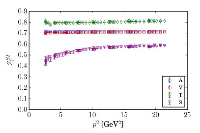
Refer to caption
Figure 9: Scale-independent renormalization factors for vector, scalar, and tensor currents. The axial current renormalization ZAsubscript𝑍𝐴Z_{A} is trivially constant because its vertex is used to eliminate the quark field renormalization Zqsubscript𝑍𝑞Z_{q}. The close values of the vector and axial-vector renormalization constants indicate that chiral symmetry-breaking effects are negligible.

The value of the lattice renormalization constants ZI(p)subscript𝑍𝐼𝑝Z_{I}(p) may depend on the orientation of the momentum p𝑝p with respect to the lattice axes due to discretization effects. We compute the lattice vertex functions (67) for various orientations of lattice momenta interpolating between 3d-diagonal and 4d-diagonal orientations to study these effects in the following sections.

V.2 Perturbative running

In order to convert operator normalization from the RI-MOM scheme discussed above to MS¯¯MS\overline{\text{MS}}, perturbative matching calculations are required. To extract lattice renormalization factors independent from the momentum subtraction point p𝑝p, the lattice factors (70) are compared to the perturbative predictions for the RI-MOM scheme in some window pmin|p|pmaxsubscript𝑝min𝑝subscript𝑝maxp_{\text{min}}\leq|p|\leq p_{\text{max}} where lattice artifacts are believed to be under control. In this section, details of relevant perturbative results are summarized.

The one-loop anomalous dimensions of the operators (7-9) were computed in Ref. Caswell et al. (1983), and the MS¯¯MS\overline{\text{MS}} anomalous dimensions to the O(αS2)𝑂superscriptsubscript𝛼𝑆2O(\alpha_{S}^{2}) precision together with O(αS)𝑂subscript𝛼𝑆O(\alpha_{S}) conversion factors were computed in Ref. Buchoff and Wagman (2016). In the chiral basis, the perturbative renormalization of the operators is diagonal (no mixing), and their independent anomalous dimensions are

1ZIddlnμZI=γI(αS)=γI(0)(αS(μ)4π)γI(1)(αS(μ)4π)2,1subscript𝑍𝐼𝑑𝑑𝜇subscript𝑍𝐼subscript𝛾𝐼subscript𝛼𝑆superscriptsubscript𝛾𝐼0subscript𝛼𝑆𝜇4𝜋superscriptsubscript𝛾𝐼1superscriptsubscript𝛼𝑆𝜇4𝜋2\frac{1}{Z_{I}}\,\frac{d}{d\,\ln\mu}Z_{I}=-\gamma_{I}(\alpha_{S})=-\gamma_{I}^{(0)}\left(\frac{\alpha_{S}(\mu)}{4\pi}\right)-\gamma_{I}^{(1)}\left(\frac{\alpha_{S}(\mu)}{4\pi}\right)^{2}\,, (72)

with the coefficients γI(0)superscriptsubscript𝛾𝐼0\gamma_{I}^{(0)} given in Tab. 1. These anomalous dimensions are substantially different, which would complicate operator renormalization if chiral symmetry was violated by a lattice fermion action and mixing was allowed. We integrate the equations (72) together with an RG equation for the coupling constant αS(μ)subscript𝛼𝑆𝜇\alpha_{S}(\mu) using the 4-loop β(αS)𝛽subscript𝛼𝑆\beta(\alpha_{S})-function. Since our lattice QCD action has Nf=2+1subscript𝑁𝑓21N_{f}=2+1 dynamical flavors, the lattice factors (70) are matched to ZRI(μ)superscript𝑍𝑅𝐼𝜇Z^{RI}(\mu) factors computed in Nf=3subscript𝑁𝑓3N_{f}=3 perturbative QCD and the coupling constant αSNf=3superscriptsubscript𝛼𝑆subscript𝑁𝑓3\alpha_{S}^{N_{f}=3} is matched to its physical value at μmc𝜇subscript𝑚𝑐\mu\leq m_{c}. The latter is obtained from a global fit Bethke (2009) and matched at the mb,csubscript𝑚𝑏𝑐m_{b,c} quark mass thresholds. For the reference point μ0=2GeVsubscript𝜇02GeV\mu_{0}=2\,\text{GeV}, its values999 The coupling constant in the RI-MOM scheme is conveniently defined to be equal to the MS¯¯MS\overline{\text{MS}} coupling constant. are αSNf=3=0.2827superscriptsubscript𝛼𝑆subscript𝑁𝑓30.2827\alpha_{S}^{N_{f}=3}=0.2827 and αSNf=4=0.2948superscriptsubscript𝛼𝑆subscript𝑁𝑓40.2948\alpha_{S}^{N_{f}=4}=0.2948.

Refer to caption
Figure 10: Perturbative running of the operators QIsubscript𝑄𝐼Q_{I} at the 2-loop level Buchoff and Wagman (2016) in the RI-MOM scheme with Nf=3subscript𝑁𝑓3N_{f}=3 (solid) and Nf=4subscript𝑁𝑓4N_{f}=4 (dotted) and in the MS¯¯MS\overline{\text{MS}} scheme with Nf=3subscript𝑁𝑓3N_{f}=3 (dashed) and Nf=4subscript𝑁𝑓4N_{f}=4 (dash-dotted). The 1-loop results are shown with thin solid lines. The reference point is μ1=1.5GeVmcsubscript𝜇11.5GeVsubscript𝑚𝑐\mu_{1}=1.5\,\text{GeV}\approx m_{c}.

The final results are converted to Nf=4subscript𝑁𝑓4N_{f}=4 QCD at μ0=2GeVsubscript𝜇02GeV\mu_{0}=2\,\text{GeV}, again matching at the mcsubscript𝑚𝑐m_{c} threshold. The final conversion factors from lattice to the MS¯¯MS\overline{\text{MS}} scheme at scale μ0subscript𝜇0\mu_{0} are

CIMS¯(Nf=4)lat(μ0)=[ZIMS¯(Nf=4)(μ0)ZIMS¯(Nf=4)(mc)]pert[ZIMS¯(Nf=3)(μ0)ZIMS¯(Nf=3)(mc)]pert1CIMS¯RI(Nf=3)(μ0)ZISI(μ0,a),superscriptsubscript𝐶𝐼¯MSsubscript𝑁𝑓4latsubscript𝜇0subscriptdelimited-[]superscriptsubscript𝑍𝐼¯MSsubscript𝑁𝑓4subscript𝜇0superscriptsubscript𝑍𝐼¯MSsubscript𝑁𝑓4subscript𝑚𝑐pertsuperscriptsubscriptdelimited-[]superscriptsubscript𝑍𝐼¯MSsubscript𝑁𝑓3subscript𝜇0superscriptsubscript𝑍𝐼¯MSsubscript𝑁𝑓3subscript𝑚𝑐pert1superscriptsubscript𝐶𝐼¯MS𝑅𝐼subscript𝑁𝑓3subscript𝜇0subscriptsuperscript𝑍𝑆𝐼𝐼subscript𝜇0𝑎C_{I}^{\overline{\text{MS}}(N_{f}=4)\leftarrow\text{lat}}(\mu_{0})=\left[\frac{Z_{I}^{\overline{\text{MS}}(N_{f}=4)}(\mu_{0})}{Z_{I}^{\overline{\text{MS}}(N_{f}=4)}(m_{c})}\right]_{\text{pert}}\left[\frac{Z_{I}^{\overline{\text{MS}}(N_{f}=3)}(\mu_{0})}{Z_{I}^{\overline{\text{MS}}(N_{f}=3)}(m_{c})}\right]_{\text{pert}}^{-1}C_{I}^{\overline{\text{MS}}\leftarrow RI(N_{f}=3)}(\mu_{0})Z^{SI}_{I}(\mu_{0},a)\,, (73)

where ZISIsubscriptsuperscript𝑍𝑆𝐼𝐼Z^{SI}_{I} is a “scale-independent” lattice renormalization factor with a reference point μ0subscript𝜇0\mu_{0} defined in the next section. The perturbative scale dependence in both the MS¯¯MS\overline{\text{MS}} and RI-MOM schemes with Nf=3subscript𝑁𝑓3N_{f}=3 and 4 flavors is shown in Fig. 10.

V.3 Fits of nonperturbative and discretization effects

With known perturbative running, we can separate scale-independent renormalization from lattice artifacts and nonperturbative effects. Correlation functions computed on a lattice are subject to discretization effects that may break rotational symmetry at short distances, which are relevant for the large momenta used in the nonperturbative renormalization. In addition, they may have nonperturbative contributions that complicate matching with perturbative calculations. Below we follow closely the analysis performed in Ref. Blossier et al. (2015) and extract the scale-invariant renormalization constants ZISIsuperscriptsubscript𝑍𝐼SIZ_{I}^{\text{SI}} from a fit

Zlat=ZISI(μ0,a)[ZIRI(|p|)ZIRI(μ0)]pert+ΔZIdisc(akp[k])+ΔZINP(p2),superscript𝑍latsubscriptsuperscript𝑍SI𝐼subscript𝜇0𝑎superscriptdelimited-[]superscriptsubscript𝑍𝐼RI𝑝superscriptsubscript𝑍𝐼RIsubscript𝜇0pertΔsuperscriptsubscript𝑍𝐼discsuperscript𝑎𝑘superscript𝑝delimited-[]𝑘Δsuperscriptsubscript𝑍𝐼𝑁𝑃superscript𝑝2Z^{\text{lat}}=Z^{\text{SI}}_{I}\big{(}\mu_{0},a\big{)}\,\left[\frac{Z_{I}^{\text{RI}}(|p|)}{Z_{I}^{\text{RI}}(\mu_{0})}\right]^{\text{pert}}+\Delta Z_{I}^{\text{disc}}\big{(}a^{k}p^{[k]}\big{)}+\Delta Z_{I}^{NP}\big{(}p^{2}\big{)}\,, (74)

where ZSI(μ0,a)superscript𝑍𝑆𝐼subscript𝜇0𝑎Z^{SI}(\mu_{0},a) is the momentum-independent lattice renormalization constant, ZIRI,pert(μ)superscriptsubscript𝑍𝐼𝑅𝐼𝑝𝑒𝑟𝑡𝜇Z_{I}^{RI,pert}(\mu) is the perturbative running of QIsubscript𝑄𝐼Q_{I} in the RI-MOM scheme and ΔZIdisc,NPΔsuperscriptsubscript𝑍𝐼disc,NP\Delta Z_{I}^{\text{disc,NP}} encapsulates discretization and nonperturbative corrections. In our calculation with O(a)𝑂𝑎O(a)-improved action, the discretization effects must scale as O((ap)2)𝑂superscript𝑎𝑝2O\big{(}(ap)^{2}\big{)},

ΔZIdisc(akpi[k])=A(ap)2+[B1(ap)2+B2(ap)4]a4p[4](ap)4Δsuperscriptsubscript𝑍𝐼discsuperscript𝑎𝑘superscript𝑝𝑖delimited-[]𝑘𝐴superscript𝑎𝑝2delimited-[]subscript𝐵1superscript𝑎𝑝2subscript𝐵2superscript𝑎𝑝4superscript𝑎4superscript𝑝delimited-[]4superscript𝑎𝑝4\displaystyle\Delta Z_{I}^{\text{disc}}(a^{k}p^{i}{[k]})=A(ap)^{2}+\big{[}B_{1}(ap)^{2}+B_{2}(ap)^{4}\big{]}\frac{a^{4}p^{[4]}}{(ap)^{4}} (75)

where we also include the hypercubic invariant p[4]proportional-toabsentsuperscript𝑝delimited-[]4\propto p^{[4]} (see Fig. 11)

p[2k]=μpμ2ksuperscript𝑝delimited-[]2𝑘subscript𝜇superscriptsubscript𝑝𝜇2𝑘p^{[2k]}=\sum_{\mu}p_{\mu}^{2k} (76)

that breaks the rotational symmetry O(4)H(4)𝑂4𝐻4O(4)\to H(4) for k0,1𝑘01k\neq 0,1.

Although the vertex functions (61) are computed with “exceptional” kinematics p𝒪=0subscript𝑝𝒪0p_{\mathcal{O}}=0 (see Fig. 7), they do not have “pole” contributions 1/p2proportional-toabsent1superscript𝑝2\propto 1/p^{2} because, unlike the pseudoscalar density operator that can couple to pions, the 6-quark operators QIsubscript𝑄𝐼Q_{I} can couple only to 2-baryon (B=2𝐵2B=2) states with masses M2mN𝑀2subscript𝑚𝑁M\geq 2m_{N}. However, the nonperturbative contributions are added to Eq. (74)

ΔZNP(p2)=Cp2,Δsuperscript𝑍𝑁𝑃superscript𝑝2𝐶superscript𝑝2\Delta Z^{NP}(p^{2})=\frac{C}{p^{2}}\,, (77)

to account for effects of the dimension-2 gluon condensate Boucaud et al. (2000, 2001); Dudal et al. (2003); Ruiz Arriola et al. (2004); Megias et al. (2006); Dudal et al. (2010); Kondo (2001) that may be present in the quark propagators used to amputate the Green’s functions. Contributions of condensates to correlation functions are scale-dependent and should be evaluated using OPE as in, e.g., Ref. Blossier et al. (2011). Such analysis has not been performed yet, and the correction in Eq. (77) should be regarded as a phenomenological assumption. Another potential source of 1/p2proportional-toabsent1superscript𝑝2\propto 1/p^{2} effects are nonperturbative infrared contributions due to potential low-momentum subdiagrams, which may appear due to the same arguments as in Ref. Aoki et al. (2008).
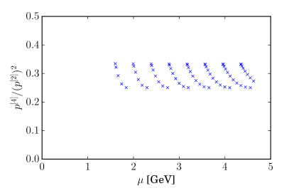
Refer to caption
Figure 11: Normalized H(4) invariant p[4]/(p2)2superscript𝑝delimited-[]4superscriptsuperscript𝑝22p^{[4]}/(p^{2})^{2} (see Eq. 76) for the lattice momenta included in the analysis.

We perform uncorrelated fit (74) with five parameters (ZISIsuperscriptsubscript𝑍𝐼SIZ_{I}^{\text{SI}}, and A,B1,2,C𝐴subscript𝐵12𝐶A,B_{1,2},C) to the lattice data ZIlat(p)superscriptsubscript𝑍𝐼lat𝑝Z_{I}^{\text{lat}}(p) for varying sets of momenta p𝑝p, and two examples are shown in Fig. 12. To keep discretization errors omitted from Eq. (75) as small as possible, we include only momenta p𝑝p that interpolate between the 3d- and 4d-diagonals,

pμsubscript𝑝𝜇\displaystyle p_{\mu} =(±k1,±k2,±k2,k2),k1k2,formulae-sequenceabsentplus-or-minussubscript𝑘1plus-or-minussubscript𝑘2plus-or-minussubscript𝑘2subscript𝑘2subscript𝑘1subscript𝑘2\displaystyle=\big{(}\pm k_{1},\pm k_{2},\pm k_{2},k_{2}\big{)}\,,\quad k_{1}\leq k_{2}\,, (78)
k1subscript𝑘1\displaystyle k_{1} =a1(0π2)=(02.7)GeV,absentsuperscript𝑎10𝜋202.7GeV\displaystyle=a^{-1}\big{(}0\ldots\frac{\pi}{2}\big{)}=\big{(}0\ldots 2.7\big{)}\text{GeV}\,,
k2subscript𝑘2\displaystyle k_{2} =a1(π6π2)=(0.92.7)GeV,absentsuperscript𝑎1𝜋6𝜋20.92.7GeV\displaystyle=a^{-1}\big{(}\frac{\pi}{6}\ldots\frac{\pi}{2}\big{)}=\big{(}0.9\ldots 2.7\big{)}\text{GeV}\,,

The lowest rotational symmetry-breaking contribution p[4]/p4proportional-toabsentsuperscript𝑝delimited-[]4superscript𝑝4\propto p^{[4]}/p^{4} to Eq. (75) is shown in Fig. 11. Values ZIlat(p)superscriptsubscript𝑍𝐼lat𝑝Z_{I}^{\text{lat}}(p) at H(4)𝐻4H(4)-equivalent momenta p𝑝p are averaged. The fit range pmin2p2pmax2superscriptsubscript𝑝min2superscript𝑝2superscriptsubscript𝑝max2p_{\text{min}}^{2}\leq p^{2}\leq p_{\text{max}}^{2} is varied with pmin=1.6, 2.0GeVsubscript𝑝min1.62.0GeVp_{\text{min}}=1.6,\,2.0\,\text{GeV} and pmax=3.5, 4.0, 4.5GeVsubscript𝑝max3.54.04.5GeVp_{\text{max}}=3.5,\,4.0,\,4.5\,\text{GeV}, resulting in 27nmom6127subscript𝑛mom6127\leq n_{\text{mom}}\leq 61 lattice momentum data points that are distinct with respect to H(4)𝐻4H(4) transformations. We use uncorrelated χ2superscript𝜒2\chi^{2} values to evaluate goodness-of-fit and estimate systematic uncertainties from variation of the results with the fit range and the order of the perturbation theory. Although correlated fits would be preferred, we resort to uncorrelated fits, because with a small number of independent configurations Ncfg=30subscript𝑁cfg30N_{\text{cfg}}=30, it is difficult to ensure that covariance matrices of sizes nmomNcfgsimilar-tosubscript𝑛momsubscript𝑁cfgn_{\text{mom}}\sim N_{\text{cfg}} are estimated with uniform reliability.
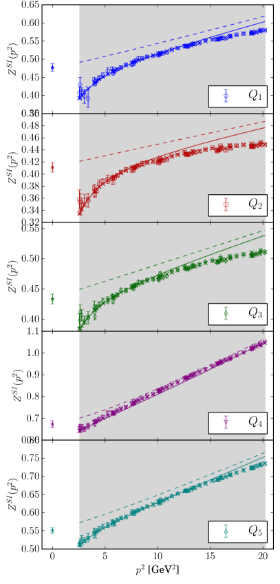
Refer to caption
Refer to caption
Figure 12: Fits of lattice renormalization constants Zlat(p)superscript𝑍lat𝑝Z^{\text{lat}}(p) to the form (74), for 1.6p4.5GeV1.6𝑝4.5GeV1.6\leq p\leq 4.5\,\text{GeV} (left) and 2.0p3.5GeV2.0𝑝3.5GeV2.0\leq p\leq 3.5\,\text{GeV} (right). For each operator, the figures show the ZSIsuperscript𝑍𝑆𝐼Z^{SI} contribution together with the (ap)2proportional-toabsentsuperscript𝑎𝑝2\propto(ap)^{2} discretization correction (dashed lines), plus the nonperturbative correction (77) (solid lines), plus the discretization corrections (75) (crosses) vs. lattice values Zlatsuperscript𝑍latZ^{\text{lat}} (open symbols). The gray bands indicate the fit regions. The star symbols on the left of each panel show the final ZSIsuperscript𝑍𝑆𝐼Z^{SI} values and their statistical uncertainties.

The results of the fits for all fit windows using ZRI,pertsuperscript𝑍𝑅𝐼𝑝𝑒𝑟𝑡Z^{RI,pert} from 1- and 2-loop perturbative calculations ZRI,pertsuperscript𝑍𝑅𝐼𝑝𝑒𝑟𝑡Z^{RI,pert} are collected in Tab. 4, together with the resulting uncorrelated χ2superscript𝜒2\chi^{2} values. In order to obtain the final value, we average the central values over all the fitting methods as described in Sec. B.3. In the last row of Table 4, we show the final conversion coefficients between the lattice bare and MS¯¯MS\overline{\text{MS}}-renormalized operators QIsubscript𝑄𝐼Q_{I} that take into account the difference between Nf=3subscript𝑁𝑓3N_{f}=3 and Nf=4subscript𝑁𝑓4N_{f}=4 QCD perturbative running (see Sec. V.2 and Eq. (73)).

Table 4: Summary of renormalization constants from fits in different q𝑞q ranges and with 1- and 2-loop QCD running, with statistical uncertainties and uncorrelated χ2superscript𝜒2\chi^{2}-values. The first two columns show the fit ranges and the perturbative orders of QCD matching. The last two rows show the wmsubscript𝑤𝑚w_{m}-weighed (112) final values with statistical and systematic uncertainties for ZISIsubscriptsuperscript𝑍𝑆𝐼𝐼Z^{SI}_{I} (74) and the conversion coefficients between the lattice bare values and the MS¯(2GeV)¯MS2GeV\overline{\text{MS}}(2\,\text{GeV}) scheme.
p[GeVp\,[\text{GeV} Zpertsuperscript𝑍pertZ^{\text{pert}} ndof Q1subscript𝑄1Q_{1} χ2superscript𝜒2\chi^{2} Q2subscript𝑄2Q_{2} χ2superscript𝜒2\chi^{2} Q3subscript𝑄3Q_{3} χ2superscript𝜒2\chi^{2} Q4subscript𝑄4Q_{4} χ2superscript𝜒2\chi^{2} Q5subscript𝑄5Q_{5} χ2superscript𝜒2\chi^{2}
1.6:3.5 1L 28 0.425(30) 31.7 0.378(36) 25.6 0.369(39) 33.8 0.615(55) 22.3 0.509(47) 27.4
2L 28 0.432(31) 32.0 0.380(37) 25.5 0.372(39) 33.9 0.646(58) 23.0 0.519(48) 27.7
1.6:4.0 1L 42 0.458(11) 37.8 0.403(14) 33.3 0.421(11) 47.1 0.605(14) 28.2 0.526(11) 35.6
2L 42 0.471(11) 38.4 0.405(14) 33.2 0.426(11) 47.9 0.650(15) 29.6 0.544(11) 37.4
1.6:4.5 1L 56 0.462(10) 69.3 0.409(08) 68.4 0.427(08) 83.8 0.622(14) 50.2 0.530(07) 62.9
2L 56 0.477(10) 72.1 0.411(08) 68.3 0.433(08) 86.1 0.673(15) 55.0 0.551(08) 68.5
2.0:3.5 1L 22 0.508(75) 24.6 0.469(61) 19.0 0.434(68) 28.9 0.763(91) 17.1 0.602(79) 21.9
2L 22 0.523(76) 24.6 0.471(62) 19.0 0.440(69) 28.9 0.826(98) 17.1 0.626(82) 21.7
2.0:4.0 1L 36 0.476(15) 30.7 0.433(17) 25.3 0.452(14) 38.0 0.638(32) 24.6 0.559(24) 29.2
2L 36 0.494(16) 30.7 0.435(17) 25.3 0.460(14) 38.4 0.698(35) 24.7 0.586(25) 29.6
2.0:4.5 1L 50 0.477(12) 60.4 0.433(10) 55.7 0.451(10) 70.4 0.656(21) 43.5 0.556(13) 53.1
2L 50 0.495(13) 62.1 0.435(10) 55.6 0.459(11) 71.7 0.720(23) 45.6 0.585(14) 55.9
ZISI(μ0)subscriptsuperscript𝑍𝑆𝐼𝐼subscript𝜇0Z^{SI}_{I}(\mu_{0}) (δstat)(δsys)superscript𝛿statsuperscript𝛿sys(\delta^{\text{stat}})(\delta^{\text{sys}}) 0.471(15)(15) 0.420(17)(17) 0.437(16)(20) 0.644(22)(35) 0.543(16)(19)
CIMS¯latsubscriptsuperscript𝐶¯MSlat𝐼C^{\overline{\text{MS}}\leftarrow\text{lat}}_{I} (δstat)(δsys)superscript𝛿statsuperscript𝛿sys(\delta^{\text{stat}})(\delta^{\text{sys}}) 0.433(14)(14) 0.429(17)(17) 0.425(15)(20) 0.520(18)(28) 0.527(15)(19)

Our lattice vertex functions (61) are computed with nonzero quark masses but matched to massless perturbation theory. Since we analyze only one ensemble, we cannot take the chiral limit mu/d,s0subscript𝑚𝑢𝑑𝑠0m_{u/d,s}\to 0 and our renormalization can potentially have systematic bias due to quark mass dependence. While the light quark masses are small and are unlikely to have significant effect, the strange quark mass is larger and it may bias our results. Although we cannot directly assess this quark mass dependence with data at only one combination of quark masses, we can make a rough estimate of its magnitude from the quark mass dependence of the axial-vector renormalization constant ZAsubscript𝑍𝐴Z_{A}. Since the operator renormalization constants in our analysis are multiplied by factors Zq3ZA3proportional-toabsentsuperscriptsubscript𝑍𝑞3proportional-tosuperscriptsubscript𝑍𝐴3\propto Z_{q}^{3}\propto Z_{A}^{3}, we can estimate their corresponding quark-mass correction as

δZIZI=3δZAZA,𝛿subscript𝑍𝐼subscript𝑍𝐼3𝛿subscript𝑍𝐴subscript𝑍𝐴\frac{\delta Z_{I}}{Z_{I}}=3\frac{\delta Z_{A}}{Z_{A}}\,, (79)

where the correction δZA𝛿subscript𝑍𝐴\delta Z_{A} due to the mu/d,s0subscript𝑚𝑢𝑑𝑠0m_{u/d,s}\to 0 limit may be conservatively estimated as

δZA=msphysmax{|ZAml|,|ZAms|}.𝛿subscript𝑍𝐴superscriptsubscript𝑚𝑠𝑝𝑦𝑠maxsubscript𝑍𝐴subscript𝑚𝑙subscript𝑍𝐴subscript𝑚𝑠\delta Z_{A}=m_{s}^{phys}\cdot\text{max}\Big{\{}\Big{|}\frac{\partial Z_{A}}{\partial m_{l}}\Big{|}\,,\Big{|}\frac{\partial Z_{A}}{\partial m_{s}}\Big{|}\Big{\}}\,. (80)

Using the data from Ref. Aoki et al. (2011) obtained with a very similar fermion action and lattice spacing, we find from Eq. (79) that δZI/ZI1.7%𝛿subscript𝑍𝐼subscript𝑍𝐼percent1.7\delta Z_{I}/Z_{I}\approx 1.7\%. Considering that this (likely overestimated) correction is small compared to the uncertainties quoted in Tab. 4, we neglect it in the present analysis.

VI Results

The four indepedent non-vanishing nn¯𝑛¯𝑛n\overline{n} matrix elements in the isospin limit are given in terms of the above bare matrix elements and renormalization factors as

IMS¯(2 GeV)=CIMS¯(Nf=4)lat(2 GeV)Ilatsuperscriptsubscript𝐼¯MS2 GeVsuperscriptsubscript𝐶𝐼¯MSsubscript𝑁𝑓4lat2 GeVsuperscriptsubscript𝐼lat\begin{split}{\mathcal{M}}_{I}^{\overline{\text{MS}}}(2\text{ GeV})=C_{I}^{\overline{\text{MS}}(N_{f}=4)\leftarrow\text{lat}}(2\text{ GeV}){\mathcal{M}}_{I}^{\text{lat}}\end{split} (81)

Combining the uncertainties from Ilatsuperscriptsubscript𝐼lat{\mathcal{M}}_{I}^{\text{lat}} and ZISIsuperscriptsubscript𝑍𝐼𝑆𝐼Z_{I}^{SI} in quadrature gives the result

1MS¯(2 GeV)=46(13)(2)×105 GeV62MS¯(2 GeV)=95(15)(7)×105 GeV63MS¯(2 GeV)=50(10)(6)×105 GeV65MS¯(2 GeV)=1.06(45)(15)×105 GeV6,superscriptsubscript1¯MS2 GeV46132superscript105superscript GeV6superscriptsubscript2¯MS2 GeV95157superscript105superscript GeV6superscriptsubscript3¯MS2 GeV50106superscript105superscript GeV6superscriptsubscript5¯MS2 GeV1.064515superscript105superscript GeV6\begin{split}{\mathcal{M}}_{1}^{\overline{\text{MS}}}(2\text{ GeV})&=-46(13)(2)\times 10^{-5}\text{ GeV}^{6}\\ {\mathcal{M}}_{2}^{\overline{\text{MS}}}(2\text{ GeV})&=95(15)(7)\times 10^{-5}\text{ GeV}^{6}\\ {\mathcal{M}}_{3}^{\overline{\text{MS}}}(2\text{ GeV})&=-50(10)(6)\times 10^{-5}\text{ GeV}^{6}\\ {\mathcal{M}}_{5}^{\overline{\text{MS}}}(2\text{ GeV})&=-1.06(45)(15)\times 10^{-5}\text{ GeV}^{6},\end{split} (82)

where the first uncertainty is the combined statistical uncertainty in Ilatsuperscriptsubscript𝐼lat{\mathcal{M}}_{I}^{\text{lat}} and ZIsubscript𝑍𝐼Z_{I} and the second uncertainty is the combined systematic uncertainty associated with variation in fit window described in Sec. IVV and Appendix B.3. Quark mass effects lead to negligible systematic uncertainties because of the nearly physical pion mass used Blum et al. (2016)101010 The renormalization constants require taking the limit mu/d,s0subscript𝑚𝑢𝑑𝑠0m_{u/d,s}\to 0 for matching to their exact perturbative counterparts. The associated uncertainty is estimated in Sec. V to be small and is neglected in the present study.. Uncertainties in the determination of the lattice spacing in Ref. Blum et al. (2016) are negligible compared to the fitting uncertainties in Eq. (82). Finite-volume effects have been estimated in chiral perturbation theory to be 1%less-than-or-similar-toabsentpercent1\lesssim 1\% effects for the volume used for this study Bijnens and Kofoed (2017). Discretization effects are expected to be the largest unquantified systematic uncertainty that are neglected in this work. Chiral symmetry leads to O(a)𝑂𝑎O(a) improvement of the fermion action, and discretization effects on meson observables for these configurations have been seen to be percent-level Blum et al. (2016). Discretization effects will be studied and removed from future calculations with multiple lattice spacing.

Final results for the n-n¯𝑛-¯𝑛n\text{-}\overline{n} transition matrix elements with statistical and systematic uncertainties added in quadrature and given in Tab. 5. These results can be directly compared with MIT bag model results previously used to relate experimental results to BSM couplings Rao and Shrock (1982) as shown in Tab. 5. Two different sets of MIT bag model parameters are used to calculate n-n¯𝑛-¯𝑛n\text{-}\overline{n} transition matrix elements in Ref. Rao and Shrock (1982): in fit A the up and down quark masses are set to zero, while in fit B the up and down quark masses are set to 108 MeV and a different value is used for the “bag radius” parameter. MIT bag model results for both fit A and fit B are compared to LQCD results in Tab. 5. In LQCD, the electroweak-nonsinglet matrix element 5subscript5{\mathcal{M}}_{5} is more than an order of magnitude smaller than the electroweak-singlet matrix elements. This feature is captured by the MIT bag model, although the sign of 5subscript5{\mathcal{M}}_{5} differs between the two bag model parametrizations. LQCD results for the electroweak-singlet operator matrix elements 1subscript1{\mathcal{M}}_{1}, 2subscript2{\mathcal{M}}_{2}, and 3subscript3{\mathcal{M}}_{3} are larger than MIT bag model results with both parametrizations by factors of 4-8. This difference between LQCD and MIT bag model results is significantly larger than the differences between MIT bag model results with different parameter values.

The effective Lagrangian for n-n¯𝑛-¯𝑛n\text{-}\overline{n} oscillations given in Eq. (46) can be used to parameterize the n-n¯𝑛-¯𝑛n\text{-}\overline{n} vacuum transition rate for a generic BSM theory as

τn-n¯1=|n-n¯|=1ΛBSM5|I=1,2,3(C~IηC~I𝒫)I+(η2C~5ηC~5𝒫)5|,superscriptsubscript𝜏𝑛-¯𝑛1subscript𝑛-¯𝑛1superscriptsubscriptΛBSM5subscript𝐼123subscript~𝐶𝐼𝜂superscriptsubscript~𝐶𝐼𝒫subscript𝐼superscript𝜂2subscript~𝐶5𝜂superscriptsubscript~𝐶5𝒫subscript5\tau_{n\text{-}\overline{n}}^{-1}=\big{|}{\mathcal{M}}_{n\text{-}\overline{n}}\big{|}=\frac{1}{\Lambda_{\text{BSM}}^{5}}\Big{|}\sum_{I=1,2,3}\Big{(}\widetilde{C}_{I}-\eta\widetilde{C}_{I}^{{\mathcal{P}}}\Big{)}{\mathcal{M}}_{I}+\Big{(}\eta^{2}\widetilde{C}_{5}-\eta\widetilde{C}_{5}^{\mathcal{P}}\Big{)}{\mathcal{M}}_{5}\Big{|}\,, (83)

where η=v2/ΛBSM2𝜂superscript𝑣2superscriptsubscriptΛBSM2\eta=v^{2}/\Lambda_{\text{BSM}}^{2} is the ratio of the Higgs v.e.v. and the BSM scale squared. Both the matrix elements {\mathcal{M}} and the Wilson coefficients C~(𝒫)superscript~𝐶𝒫\widetilde{C}^{({\mathcal{P}})} are scheme- and scale-dependent, and these dependencies must cancel in τn-n¯subscript𝜏𝑛-¯𝑛\tau_{n\text{-}\overline{n}}. Below we present results with coefficients C~~𝐶\widetilde{C} defined in MS¯¯MS\overline{\text{MS}} scheme. The Wilson coefficients in Eq. (83) are predicted to be non-zero in various BSM theories, see Refs. Mohapatra (2009); Babu et al. (2013); Phillips et al. (2016) for reviews and further references, and are calculable at tree-level in QCD at BSM scales μ=ΛBSM𝜇subscriptΛBSM\mu=\Lambda_{\text{BSM}}. The n-n¯𝑛-¯𝑛n\text{-}\overline{n} vacuum transition rate is given in terms of the above results by

τn-n¯1=(109 s1)(700 TeVΛBSM)5| 4.2(1.1)(C~1MS¯(μ)ηC~1MS¯,𝒫(μ))8.6(1.5)(C~2MS¯(μ)ηC~2MS¯,𝒫(μ))+4.5(1.1)(C~3MS¯(μ)ηC~3MS¯,𝒫(μ))+0.096(43)(η2C~5MS¯(μ)ηC~5MS¯,𝒫(μ))|μ=2 GeV.\begin{split}\tau_{n\text{-}\overline{n}}^{-1}&=(10^{-9}\text{ s}^{-1})\left(\frac{700\text{ TeV}}{\Lambda_{\text{BSM}}}\right)^{5}\Big{|}\,4.2(1.1)\Big{(}\widetilde{C}_{1}^{\overline{\text{MS}}}(\mu)-\eta\widetilde{C}_{1}^{\overline{\text{MS}},{\mathcal{P}}}(\mu)\Big{)}-8.6(1.5)\Big{(}\widetilde{C}_{2}^{\overline{\text{MS}}}(\mu)-\eta\widetilde{C}_{2}^{\overline{\text{MS}},{\mathcal{P}}}(\mu)\Big{)}\\ &\quad\quad+4.5(1.1)\Big{(}\widetilde{C}_{3}^{\overline{\text{MS}}}(\mu)-\eta\widetilde{C}_{3}^{\overline{\text{MS}},{\mathcal{P}}}(\mu)\Big{)}+0.096(43)\Big{(}\eta^{2}\widetilde{C}_{5}^{\overline{\text{MS}}}(\mu)-\eta\widetilde{C}_{5}^{\overline{\text{MS}},{\mathcal{P}}}(\mu)\Big{)}\Big{|}_{\mu=2\text{ GeV}}.\end{split} (84)

To make the prefactor dimensionless, we use the “reference” normalization scale of 700TeV700TeV700\,\text{TeV}. Estimates based on Eq. (84) put BSM theories with scales of ΛBSM700similar-tosubscriptΛBSM700\Lambda_{\text{BSM}}\sim 700 TeV and O(1)𝑂1O(1) matching coefficients within reach of next-generation experiments that will be able to detect baryon number violation with τn-n¯1109superscriptsubscript𝜏𝑛-¯𝑛1superscript109\tau_{n\text{-}\overline{n}}^{-1}\geq 10^{9}Milstead (2015); Frost (2017); Fomin et al. (2018); Hewes (2017). To more precisely assess the expected signatures of theories with B𝐵B-violation at ΛBSM700similar-tosubscriptΛBSM700\Lambda_{\text{BSM}}\sim 700 TeV, the operators can be evolved to μ=ΛBSM𝜇subscriptΛBSM\mu=\Lambda_{\text{BSM}} using the results of Refs. Caswell et al. (1983); Buchoff and Wagman (2016),

1MS¯(700 TeV)=26(7)(1)×105 GeV62MS¯(700 TeV)=144(23)(11)×105 GeV63MS¯(700 TeV)=47(9)(6)×105 GeV65MS¯(700 TeV)=0.23(10)(3)×105 GeV6.superscriptsubscript1¯MS700 TeV2671superscript105superscript GeV6superscriptsubscript2¯MS700 TeV1442311superscript105superscript GeV6superscriptsubscript3¯MS700 TeV4796superscript105superscript GeV6superscriptsubscript5¯MS700 TeV0.23103superscript105superscript GeV6\begin{split}{\mathcal{M}}_{1}^{\overline{\text{MS}}}(700\text{ TeV})&=-26(7)(1)\times 10^{-5}\text{ GeV}^{6}\\ {\mathcal{M}}_{2}^{\overline{\text{MS}}}(700\text{ TeV})&=144(23)(11)\times 10^{-5}\text{ GeV}^{6}\\ {\mathcal{M}}_{3}^{\overline{\text{MS}}}(700\text{ TeV})&=-47(9)(6)\times 10^{-5}\text{ GeV}^{6}\\ {\mathcal{M}}_{5}^{\overline{\text{MS}}}(700\text{ TeV})&=-0.23(10)(3)\times 10^{-5}\text{ GeV}^{6}.\end{split} (85)

Leading-order one-loop running from 2 GeV to 700 TeV modifies the dominant matrix elements M1,3subscript𝑀13M_{1,3} by up to 59%. At next-to-leading-order (NLO), two-loop running modifies M1,2,3subscript𝑀123M_{1,2,3} by 49%4percent94-9\% and one-loop scheme matching modifies them by 28%2percent82-8\%. Neglected next-to-next-to-leading-order perturbative renormalization effects lead to unknown systematic uncertainties estimated to be at the level of 13%1percent31-3\% (as the square of the relative NLO effects). The n-n¯𝑛-¯𝑛n\text{-}\overline{n} transition rate can be expressed in terms of the matrix elements at this scale as

τn-n¯1=(109 s1)(700 TeVΛBSM)5| 2.4(0.7)(C~1MS¯(μ)ηC~1MS¯,𝒫(μ))12.9(2.3)(C~2MS¯(μ)ηC~2MS¯,𝒫(μ))+4.2(1.0)(C~3MS¯(μ)ηC~3MS¯,𝒫(μ))+0.021(9)(η2C~5MS¯(μ)ηC~5MS¯,𝒫(μ))|μ=700 TeV.\begin{split}\tau_{n\text{-}\overline{n}}^{-1}&=(10^{-9}\text{ s}^{-1})\left(\frac{700\text{ TeV}}{\Lambda_{\text{BSM}}}\right)^{5}\Big{|}\,2.4(0.7)\Big{(}\widetilde{C}_{1}^{\overline{\text{MS}}}(\mu)-\eta\widetilde{C}_{1}^{\overline{\text{MS}},{\mathcal{P}}}(\mu)\Big{)}-12.9(2.3)\Big{(}\widetilde{C}_{2}^{\overline{\text{MS}}}(\mu)-\eta\widetilde{C}_{2}^{\overline{\text{MS}},{\mathcal{P}}}(\mu)\Big{)}\\ &\quad\quad+4.2(1.0)\Big{(}\widetilde{C}_{3}^{\overline{\text{MS}}}(\mu)-\eta\widetilde{C}_{3}^{\overline{\text{MS}},{\mathcal{P}}}(\mu)\Big{)}+0.021(9)\Big{(}\eta^{2}\widetilde{C}_{5}^{\overline{\text{MS}}}(\mu)-\eta\widetilde{C}_{5}^{\overline{\text{MS}},{\mathcal{P}}}(\mu)\Big{)}\Big{|}_{\mu=700\text{ TeV}}.\end{split} (86)

This result can be combined with tree-level BSM matching results for CIMS¯(700 TeV)superscriptsubscript𝐶𝐼¯MS700 TeVC_{I}^{\overline{\text{MS}}}(700\text{ TeV}) to extract constraints on BSM theory parameters from experimental constraints on n-n¯𝑛-¯𝑛n\text{-}\overline{n} oscillations.

Operator IMS¯(2 GeV),superscriptsubscript𝐼¯MS2 GeV{\mathcal{M}}_{I}^{\overline{\text{MS}}}(2\text{ GeV}), IMS¯(700 TeV),superscriptsubscript𝐼¯MS700 TeV{\mathcal{M}}_{I}^{\overline{\text{MS}}}(700\text{ TeV}), IMS¯(2 GeV)MIT bag Asuperscriptsubscript𝐼¯MS2 GeVMIT bag A\frac{{\mathcal{M}}_{I}^{\overline{\text{MS}}}(2\text{ GeV})}{\text{MIT bag A}} IMS¯(2 GeV)MIT bag Bsuperscriptsubscript𝐼¯MS2 GeVMIT bag B\frac{{\mathcal{M}}_{I}^{\overline{\text{MS}}}(2\text{ GeV})}{\text{MIT bag B}}
Q1subscript𝑄1Q_{1} 46(13)×105 GeV64613superscript105superscript GeV6-46(13)\times 10^{-5}\text{ GeV}^{6} 26(7)×105 GeV6267superscript105superscript GeV6-26(7)\times 10^{-5}\text{ GeV}^{6} 4.2 5.2
Q2subscript𝑄2Q_{2} 95(17)×105 GeV69517superscript105superscript GeV695(17)\times 10^{-5}\text{ GeV}^{6} 144(26)×105 GeV614426superscript105superscript GeV6144(26)\times 10^{-5}\text{ GeV}^{6} 7.5 8.7
Q3subscript𝑄3Q_{3} 50(12)×105 GeV65012superscript105superscript GeV6-50(12)\times 10^{-5}\text{ GeV}^{6} 47(11)×105 GeV64711superscript105superscript GeV6-47(11)\times 10^{-5}\text{ GeV}^{6} 5.1 6.1
Q5subscript𝑄5Q_{5} 1.06(48)×105 GeV61.0648superscript105superscript GeV6-1.06(48)\times 10^{-5}\text{ GeV}^{6} 0.23(10)×105 GeV60.2310superscript105superscript GeV6-0.23(10)\times 10^{-5}\text{ GeV}^{6} -0.84 1.6
Table 5: Matrix element results for the chiral basis operators with independent non-zero matrix elements in the isospin limit. The second column shows the renormalized matrix elements at a scale of 2 GeV and total uncertainty including statistical and systematic uncertainties from the bare matrix elements and non-perturbative renormalization factor added in quadrature. Renormalized results use the MS¯¯MS\overline{\text{MS}} scheme with Nf=4subscript𝑁𝑓4N_{f}=4 active quark flavors and are obtained through nonperturbative RI-MOM renormalization and perturbative matching to MS¯¯MS\overline{\text{MS}}. The third column shows the corresponding MS¯¯MS\overline{\text{MS}} renormalized matrix elements and uncertainties after renormalization group evolution from 2 GeV to a higher scale of 700 TeV. The fourth and fifth columns show comparisons with the results of the same matrix elements in the MIT bag model from Ref. Rao and Shrock (1982) as described in the main text.

VII Conclusion

We have performed the first lattice QCD calculation of the renormalized neutron-antineutron transition matrix elements needed to extract BSM physics constraints from n-n¯𝑛-¯𝑛n\text{-}\overline{n} oscillation experiments. The precision of our final results including statistical and most systematic uncertainties is 1530%15percent3015-30\% for the electroweak-singlet matrix elements 1subscript1{\mathcal{M}}_{1}, 2subscript2{\mathcal{M}}_{2}, and 3subscript3{\mathcal{M}}_{3}, which can be straightforwardly improved in future calculations. Several important sources of systematic uncertainty are under control for the first time, most importantly non-perturbative renormalization, chiral symmetry violations, excited state contamination, and quark mass dependence. The two sources of systematic uncertainty that are not completely controlled in this pioneering calculation are finite volume and discretization effects. To summarize our control of common systematic uncertainties in lattice calculations:

  • The (nearly exact) physical pion mass mπ=139.2(4)MeVsubscript𝑚𝜋139.24MeVm_{\pi}=139.2(4)\text{MeV} in our calculation eliminates the need for chiral extrapolation, which would otherwise introduce systematic uncertainties associated with low-energy effective theory. In addition, the large difference of our results from the MIT bag model may have a similar origin as the strong suppression of proton decay matrix elements found in the chiral bag model Martin and Stavenga (2012), therefore using the realistic light quark masses in our calculation is arguably the most important systematic effect we have under control.

  • The chirally symmetric Möbius domain wall fermion action used to generate these gauge field ensembles by the RBC/UKQCD collaborations Blum et al. (2016) and compute neutron-antineutron matrix elements in this work ensures that the 14 distinct |ΔB|=2Δ𝐵2|\Delta B|=2 operators do not mix with each other and renormalization and conversion of lattice operators to MS¯¯MS\overline{\text{MS}} scheme is free from associated uncertainties. In particular, the nonperturbatively computed operator mixing matrix in RI-MOM scheme is diagonal up to O(103)𝑂superscript103O(10^{-3}) corrections, which are two orders of magnitude below other uncertainties and can be safely neglected. The identical action is used for valence quarks, so this is a fully unitary calculation.

  • Excited-state effects are accounted for using correlated two-state fits with 10 different values of tsepsubscript𝑡sept_{\text{sep}} and different combinations of nucleon source and sink smearing. The energy gaps are extracted from correlated fits to nucleon two-point functions. Since we have limited statistics for such a large number of τ,tsep𝜏subscript𝑡sep\tau,t_{\text{sep}} points included in correlated fits, we use “shrinkage” estimators to obtain well-conditioned covariance matrices. We obtain systematic errors by varying the fit ranges and averaging their results weighted by the quality-of-fit figure.

  • Renormalization effects are included through NPR in an RI-MOM scheme as described in Sec. V and one-loop matching to MS¯¯MS\overline{\text{MS}} using the results of Ref. Buchoff and Wagman (2016). Some discretization effects in NPR results such as rotational symmetry breaking and (ap)2superscript𝑎𝑝2(ap)^{2} dependence are studied and removed by fitting the lattice data with different quark momentum scales and orientations, varying scale ranges, and comparing to 1- and 2-loop perturbative QCD running. One presently uncontrolled systematic uncertainty in our renormalization procedure is the quark mass dependence. However, a rough estimate in Sec. V suggests that this uncertainty should not exceed 1.7%percent1.71.7\%, which is below our current level of precision; this uncertainty will be studied in the future.

  • Although we do not control finite-volume effects directly in this study on a single ensemble, we expect them to be small. First, finite-volume effects are suppressed with emπLsuperscript𝑒subscript𝑚𝜋𝐿e^{-m_{\pi}L} where mπL3.9similar-tosubscript𝑚𝜋𝐿3.9m_{\pi}L\sim 3.9 for the volume used for this study, which is generally considered sufficiently large for nucleon structure calculations Aoki et al. (2017). Second, chiral perturbation theory calculations in Ref. Bijnens and Kofoed (2017) estimate that finite-volume effects lead to corrections below 1%percent11\% to Isubscript𝐼{\mathcal{M}}_{I} for the volume used in this study. Future lattice calculations at additional volumes could be used to test this prediction and perform an infinite-volume extrapolation.

  • Discretization effects are the least-controlled systematic uncertainty in our current work. Lattice QCD calculations with finer lattice spacing(s) in the immediate future will be used to fully quantify and remove discretization effects that are not controlled in this calculation. However, it is reasonable to assume that discretization effects are small compared to our current combined uncertainty from other sources. First, the chirally-symmetric fermion action that we use is automatically O(a)𝑂𝑎O(a)-improved. Second, the meson decay constants computed on this ensemble (before finite volume and discretization corrections are applied) are within 0.6% of the physical values (fπ=131.1(4),fK=156.4(4)GeVformulae-sequencesubscript𝑓𝜋131.14subscript𝑓𝐾156.44GeVf_{\pi}=131.1(4),\,f_{K}=156.4(4)\,\text{GeV} Blum et al. (2016) compared to PDG values fπ=130.4(2),fK=156.2(7)GeVformulae-sequencesubscript𝑓𝜋130.42subscript𝑓𝐾156.27GeVf_{\pi}=130.4(2),\,f_{K}=156.2(7)\,\text{GeV} Olive et al. (2014)). Finally, the nucleon effective mass and energy dependence on the momentum is in close agreement with the continuum limit Syritsyn et al. (2019).

Our renormalized lattice QCD results for n-n¯𝑛-¯𝑛n\text{-}\overline{n} transition matrix elements provide a significant step forward in accuracy and reliability compared to previous results from quark models and preliminary lattice studies. The matrix elements predicted by QCD are found to be 4-8 times larger than the predictions of the MIT bag model for the dominant electroweak-singlet operators. This difference between our lattice results and previously available bag model results is much larger than the statistical or systematic uncertainties present in this calculation and is also much larger than the expected size of finite-volume effects that have not yet been studied directly. There is less certainty about the size of discretization artifacts; however, the automatic O(a)𝑂𝑎O(a) improvement due to the chiral symmetry as well as minuscule discretization corrections in the meson decay constants, nucleon mass and dispersion relation make large discretization effects in the n-n¯𝑛-¯𝑛n\text{-}\overline{n} matrix elements very unlikely.

The difference in Isubscript𝐼{\mathcal{M}}_{I} between the bag model and our lattice results leads to increased experimental sensitivity to baryon-number violating interactions that may cause n-n¯𝑛-¯𝑛n\text{-}\overline{n} oscillations. Numbers of events that can be observed both in quasi-free neutron oscillation experiments and underground nuclear decay experiments are proportional to τn-n¯2|I|2proportional-tosuperscriptsubscript𝜏𝑛-¯𝑛2superscriptsubscript𝐼2\tau_{n\text{-}\overline{n}}^{-2}\propto|{\mathcal{M}}_{I}|^{2}, therefore the ×(48)absent48\times(4\ldots 8) larger values of the n-n¯𝑛-¯𝑛n\text{-}\overline{n} matrix elements found in our work lead to ×(1664)absent1664\times(16\ldots 64) increase in the event rates. Since our results are obtained from ab initio QCD calculations in a model-independent way, they must be used for more precise assessments of the potential of planned n-n¯𝑛-¯𝑛n\text{-}\overline{n} oscillation searches as well as stronger constraints on theories of baryon-number violation and baryogenesis in the future.

Acknowledgements.
The authors would like to express gratitude to Yuri Kamyshkov, Rabi Mohapatra, Martin Savage, Steve Sharpe, Robert Shrock, Mike Snow, Brian Tiburzi for multiple illuminating discussions. We are indebted to Norman Christ, Bob Mawhinney, Taku Izubuchi, Oliver Witzel, and the rest of the RBC/UKQCD collaboration for access to the physical point domain-wall lattice gauge configurations used in this work. This work has been supported by the U. S. Department of Energy under grant contract no. DE-FG02-00ER41132 (INT). This work was performed also under the auspices of the U.S. Department of Energy by Lawrence Livermore National Laboratory (Lawrence Livermore National Security, LLC) under contract DE-AC52-07NA27344; and Brookhaven National Laboratory supported by the U. S. Department of Energy under contract DE-SC0012704. ER is supported by the RIKEN Special Postdoctoral Researcher fellowship. SS is supported by the RHIC Physics Fellow Program of the RIKEN BNL Research Center. MLW was supported by a MIT Pappalardo Fellowship and acknowledges support by the U.S. Department of Energy, Office of Science, Office of Nuclear Physics under grant Contract Number DE-SC0011090. Quark propagators and contractions were computed using the USQCD computing resources at Fermilab funded by the Office of Science of the US Department of Energy, as well as computing resources at the Lawrence Livermore National Laboratory made available through the Institutional Computing Grand Challenge program. This research used resources of the Argonne Leadership Computing Facility, which is a DOE Office of Science User Facility supported under Contract DE-AC02-06CH11357 The calculations were performed using Chroma Edwards and Joo (2005) and Qlua Pochinsky (senta) software packages, in particular with the efficient MDWF inverter developed by A. Pochinsky Pochinsky (sentb).

References

Appendix A 𝒞𝒞{\mathcal{C}}-, 𝒫𝒫{\mathcal{P}}-, 𝒯𝒯{\mathcal{T}}-symmetries and nucleon states

Fermion field transformations under 𝒞𝒞{\mathcal{C}}, 𝒫𝒫{\mathcal{P}}, and 𝒯𝒯{\mathcal{T}} are given by

𝒫ψx𝒫1𝒫subscript𝜓𝑥superscript𝒫1\displaystyle{\mathcal{P}}\psi_{x}{\mathcal{P}}^{-1} =ηPγ4ψ𝒫(x),absentsubscript𝜂𝑃subscript𝛾4subscript𝜓𝒫𝑥\displaystyle=\phantom{+}\eta_{P}\gamma_{4}\psi_{{\mathcal{P}}(x)}\,, 𝒫ψ¯x𝒫1𝒫subscript¯𝜓𝑥superscript𝒫1\displaystyle{\mathcal{P}}\bar{\psi}_{x}{\mathcal{P}}^{-1} =ηPψ¯𝒫(x)γ4,absentsuperscriptsubscript𝜂𝑃subscript¯𝜓𝒫𝑥subscript𝛾4\displaystyle=\phantom{+}\eta_{P}^{*}\bar{\psi}_{{\mathcal{P}}(x)}\gamma_{4}\,, (87)
𝒞ψx𝒞1𝒞subscript𝜓𝑥superscript𝒞1\displaystyle{\mathcal{C}}\psi_{x}{\mathcal{C}}^{-1} =ηCCψ¯xT,absentsubscript𝜂𝐶𝐶superscriptsubscript¯𝜓𝑥𝑇\displaystyle=\phantom{+}\eta_{C}C\bar{\psi}_{x}^{T}\,, 𝒞ψ¯x𝒞1𝒞subscript¯𝜓𝑥superscript𝒞1\displaystyle{\mathcal{C}}\bar{\psi}_{x}{\mathcal{C}}^{-1} =ηCψxTC,absentsuperscriptsubscript𝜂𝐶superscriptsubscript𝜓𝑥𝑇𝐶\displaystyle=\phantom{+}\eta_{C}^{*}\psi_{x}^{T}C\,, (88)
𝒯ψx𝒯1𝒯subscript𝜓𝑥superscript𝒯1\displaystyle{\mathcal{T}}\psi_{x}{\mathcal{T}}^{-1} =ηTTψT(x),absentsubscript𝜂𝑇𝑇subscript𝜓𝑇𝑥\displaystyle=\phantom{+}\eta_{T}T\psi_{T(x)}\,, 𝒯ψ¯x𝒯1𝒯subscript¯𝜓𝑥superscript𝒯1\displaystyle{\mathcal{T}}\bar{\psi}_{x}{\mathcal{T}}^{-1} =ηTψ¯𝒯(x)T,absentsuperscriptsubscript𝜂𝑇subscript¯𝜓𝒯𝑥𝑇\displaystyle=-\eta_{T}^{*}\bar{\psi}_{{\mathcal{T}}(x)}T\,, (89)

where C𝐶C is given in Eq. (4) and the spin matrix T𝑇T is

T=[γ1γ3]uc=T=TT=T=T1,𝑇subscriptdelimited-[]subscript𝛾1subscript𝛾3𝑢𝑐superscript𝑇superscript𝑇𝑇superscript𝑇superscript𝑇1T=[\gamma_{1}\gamma_{3}]_{\mathcal{E}uc}=T^{*}=-T^{T}=-T^{\dagger}=-T^{-1}\,, (90)

and has the property

TγμT=γμ,TσμνT1=σμν.formulae-sequence𝑇superscriptsubscript𝛾𝜇superscript𝑇subscript𝛾𝜇𝑇superscriptsubscript𝜎𝜇𝜈superscript𝑇1subscript𝜎𝜇𝜈T\gamma_{\mu}^{*}T^{\dagger}=\gamma_{\mu}\,,\quad T\sigma_{\mu\nu}^{*}T^{-1}=-\sigma_{\mu\nu}\,. (91)

Both the color-symmetric and antisymmetric quark bilinears transform as

𝒫(ψTCPR,Lψ)𝒫1𝒫superscript𝜓𝑇𝐶subscript𝑃𝑅𝐿𝜓superscript𝒫1\displaystyle{\mathcal{P}}(\psi^{T}CP_{R,L}\psi){\mathcal{P}}^{-1} =ηP2(ψTCPL,Rψ),absentsuperscriptsubscript𝜂𝑃2superscript𝜓𝑇𝐶subscript𝑃𝐿𝑅𝜓\displaystyle=-\eta_{P}^{2}(\psi^{T}CP_{L,R}\psi)\,, (92)
𝒞(ψTCPR,Lψ)𝒞1𝒞superscript𝜓𝑇𝐶subscript𝑃𝑅𝐿𝜓superscript𝒞1\displaystyle{\mathcal{C}}(\psi^{T}CP_{R,L}\psi){\mathcal{C}}^{-1} =ηC2(ψ¯CPL,Rψ¯T)=±ηC2(ψTCPR,Lψ),absentsuperscriptsubscript𝜂𝐶2¯𝜓𝐶subscript𝑃𝐿𝑅superscript¯𝜓𝑇plus-or-minussuperscriptsubscript𝜂𝐶2superscriptsuperscript𝜓𝑇𝐶subscript𝑃𝑅𝐿𝜓\displaystyle=\eta_{C}^{2}(\bar{\psi}CP_{L,R}\bar{\psi}^{T})=\pm\eta_{C}^{2}(\psi^{T}CP_{R,L}\psi)^{{\dagger}}\,, (93)
𝒯(ψTCPR,Lψ)𝒯1𝒯superscript𝜓𝑇𝐶subscript𝑃𝑅𝐿𝜓superscript𝒯1\displaystyle{\mathcal{T}}(\psi^{T}CP_{R,L}\psi){\mathcal{T}}^{-1} =ηT2(ψTCPL,Rψ),absentsuperscriptsubscript𝜂𝑇2superscript𝜓𝑇𝐶subscript𝑃𝐿𝑅𝜓\displaystyle=\eta_{T}^{2}(\psi^{T}CP_{L,R}\psi)\,, (94)

from which the transformation properties for the 6-quark operators (35-37) follow.

In order to find the effect of these symmetries on the nucleon states and matrix elements of the operators, we spell out explicitly the neutron interpolating operators,

nα(±)subscriptsuperscript𝑛plus-or-minus𝛼\displaystyle n^{(\pm)}_{\alpha} =εijk(uiTCγ51±γ42dj)dk,absentsuperscript𝜀𝑖𝑗𝑘superscriptsubscript𝑢𝑖𝑇𝐶subscript𝛾5plus-or-minus1subscript𝛾42subscript𝑑𝑗subscript𝑑𝑘\displaystyle=\varepsilon^{ijk}(u_{i}^{T}C\gamma_{5}\frac{1\pm\gamma_{4}}{2}d_{j})\,d_{k}\,, (95)
n¯α(±)subscriptsuperscript¯𝑛plus-or-minus𝛼\displaystyle\bar{n}^{(\pm)}_{\alpha} =(nγ4)α=εijkd¯k(d¯jCγ51±γ42u¯iT),absentsubscriptsuperscript𝑛subscript𝛾4𝛼superscript𝜀𝑖𝑗𝑘subscript¯𝑑𝑘subscript¯𝑑𝑗superscript𝐶subscript𝛾5plus-or-minus1subscript𝛾42subscriptsuperscript¯𝑢𝑇𝑖\displaystyle=(n^{\dagger}\gamma_{4})_{\alpha}=\varepsilon^{ijk}\bar{d}_{k}\,(\bar{d}_{j}C^{\dagger}\gamma_{5}\frac{1\pm\gamma_{4}}{2}\bar{u}^{T}_{i})\,,

which transform as

𝒫nx(±)𝒫1𝒫subscriptsuperscript𝑛plus-or-minus𝑥superscript𝒫1\displaystyle{\mathcal{P}}n^{(\pm)}_{x}{\mathcal{P}}^{-1} =ηP3γ4n𝒫(x)(±),absentsuperscriptsubscript𝜂𝑃3subscript𝛾4subscriptsuperscript𝑛plus-or-minus𝒫𝑥\displaystyle=\phantom{+}\eta_{P}^{3}\gamma_{4}n^{(\pm)}_{{\mathcal{P}}(x)}\,, 𝒫n¯x(±)𝒫1𝒫subscriptsuperscript¯𝑛plus-or-minus𝑥superscript𝒫1\displaystyle{\mathcal{P}}\bar{n}^{(\pm)}_{x}{\mathcal{P}}^{-1} =ηP3n¯𝒫(x)(±)γ4,absentsuperscriptsubscript𝜂𝑃absent3subscriptsuperscript¯𝑛plus-or-minus𝒫𝑥subscript𝛾4\displaystyle=\phantom{+}\eta_{P}^{*3}\bar{n}^{(\pm)}_{{\mathcal{P}}(x)}\gamma_{4}\,, (96)
𝒞nx(±)𝒞1𝒞subscriptsuperscript𝑛plus-or-minus𝑥superscript𝒞1\displaystyle{\mathcal{C}}n^{(\pm)}_{x}{\mathcal{C}}^{-1} =ηC3Cn¯x()T,absentsuperscriptsubscript𝜂𝐶3𝐶subscriptsuperscript¯𝑛minus-or-plus𝑇𝑥\displaystyle=-\eta_{C}^{3}C\bar{n}^{(\mp)T}_{x}\,, 𝒞n¯x(±)𝒞1𝒞subscriptsuperscript¯𝑛plus-or-minus𝑥superscript𝒞1\displaystyle{\mathcal{C}}\bar{n}^{(\pm)}_{x}{\mathcal{C}}^{-1} =ηC3nx()TC,absentsuperscriptsubscript𝜂𝐶absent3subscriptsuperscript𝑛minus-or-plus𝑇𝑥𝐶\displaystyle=-\eta_{C}^{*3}n^{(\mp)T}_{x}C\,,
𝒯nx(±)𝒯1𝒯subscriptsuperscript𝑛plus-or-minus𝑥superscript𝒯1\displaystyle{\mathcal{T}}n^{(\pm)}_{x}{\mathcal{T}}^{-1} =ηT3TnT(x)(±),absentsuperscriptsubscript𝜂𝑇3𝑇subscriptsuperscript𝑛plus-or-minus𝑇𝑥\displaystyle=\phantom{+}\eta_{T}^{3}Tn^{(\pm)}_{T(x)}\,, 𝒯n¯x(±)𝒯1𝒯subscriptsuperscript¯𝑛plus-or-minus𝑥superscript𝒯1\displaystyle{\mathcal{T}}\bar{n}^{(\pm)}_{x}{\mathcal{T}}^{-1} =ηT3n¯𝒯(x)(±)T.absentsuperscriptsubscript𝜂𝑇absent3subscriptsuperscript¯𝑛plus-or-minus𝒯𝑥𝑇\displaystyle=-\eta_{T}^{*3}\bar{n}^{(\pm)}_{{\mathcal{T}}(x)}T\,.

which are used to construct (anti)neutron states on a lattice. This construction is more natural in the standard (Dirac-Pauli) basis in which the γ4subscript𝛾4\gamma_{4} matrix is diagonal. It is related to the de Grand–Rossi basis commonly used in lattice calculations by the transformation

ψstd=12(11111111)ψdGRsubscript𝜓std12missing-subexpression1missing-subexpression11missing-subexpression1missing-subexpressionmissing-subexpression1missing-subexpression11missing-subexpression1missing-subexpressionsubscript𝜓dGR\psi_{\text{std}}=\frac{1}{\sqrt{2}}\left(\begin{array}[]{rrrr}&-1&&-1\\ 1&&1&\\ &1&&-1\\ -1&&1&\end{array}\right)\psi_{\text{dGR}} (97)

The operators (95) create the neutron and antineutron states with definite z^^𝑧\hat{z}-spin as

|n+1/2(+)ketsubscriptsuperscript𝑛12\displaystyle\left|{n^{(+)}_{+1/2}}\right> =n1(+)|vac,absentsuperscriptsubscript𝑛1ketvac\displaystyle=\phantom{+}n_{1}^{(+){\dagger}}\left|\text{vac}\right>\,, |n¯+1/2()ketsubscriptsuperscript¯𝑛12\displaystyle\left|{\bar{n}^{(-)}_{+1/2}}\right> =n4()|vac,absentsubscriptsuperscript𝑛4ketvac\displaystyle=-n^{(-)}_{4}\left|\text{vac}\right>\,, (98)
|n1/2(+)ketsubscriptsuperscript𝑛12\displaystyle\left|{n^{(+)}_{-1/2}}\right> =n2(+)|vac,absentsuperscriptsubscript𝑛2ketvac\displaystyle=\phantom{+}n_{2}^{(+){\dagger}}\left|\text{vac}\right>\,, |n¯1/2()ketsubscriptsuperscript¯𝑛12\displaystyle\left|{\bar{n}^{(-)}_{-1/2}}\right> =n¯3()|vac,absentsubscriptsuperscript¯𝑛3ketvac\displaystyle=\phantom{+}\bar{n}^{(-)}_{3}\left|\text{vac}\right>\,,

which can be found to transform as

𝒫|n±1/2(+)𝒫ketsubscriptsuperscript𝑛plus-or-minus12\displaystyle{\mathcal{P}}\left|{n^{(+)}_{\pm 1/2}}\right> =ηP3|n±1/2(+),absentsuperscriptsubscript𝜂𝑃absent3ketsubscriptsuperscript𝑛plus-or-minus12\displaystyle=\phantom{+}\eta_{P}^{*3}\left|{n^{(+)}_{\pm 1/2}}\right>\,, 𝒫|n¯±1/2()𝒫ketsubscriptsuperscript¯𝑛plus-or-minus12\displaystyle{\mathcal{P}}\left|{\bar{n}^{(-)}_{\pm 1/2}}\right> =ηP3|n¯±1/2(),absentsuperscriptsubscript𝜂𝑃3ketsubscriptsuperscript¯𝑛plus-or-minus12\displaystyle=-\eta_{P}^{3}\left|{\bar{n}^{(-)}_{\pm 1/2}}\right>\,, (99)
𝒞|n±1/2(+)𝒞ketsubscriptsuperscript𝑛plus-or-minus12\displaystyle{\mathcal{C}}\left|{n^{(+)}_{\pm 1/2}}\right> =ηC3|n¯±1/2(),absentsuperscriptsubscript𝜂𝐶absent3ketsubscriptsuperscript¯𝑛plus-or-minus12\displaystyle=-\eta_{C}^{*3}\left|{\bar{n}^{(-)}_{\pm 1/2}}\right>\,, 𝒞|n¯±1/2()𝒞ketsubscriptsuperscript¯𝑛plus-or-minus12\displaystyle{\mathcal{C}}\left|{\bar{n}^{(-)}_{\pm 1/2}}\right> =ηC3|n±1/2(+),absentsuperscriptsubscript𝜂𝐶3ketsubscriptsuperscript𝑛plus-or-minus12\displaystyle=-\eta_{C}^{3}\left|{n^{(+)}_{\pm 1/2}}\right>\,,
𝒯|n±1/2(+)𝒯ketsubscriptsuperscript𝑛plus-or-minus12\displaystyle{\mathcal{T}}\left|{n^{(+)}_{\pm 1/2}}\right> =ηT3|n1/2(+),absentminus-or-plussuperscriptsubscript𝜂𝑇absent3ketsubscriptsuperscript𝑛minus-or-plus12\displaystyle=\mp\eta_{T}^{*3}\left|{n^{(+)}_{\mp 1/2}}\right>\,, 𝒯|n¯±1/2()𝒯ketsubscriptsuperscript¯𝑛plus-or-minus12\displaystyle{\mathcal{T}}\left|{\bar{n}^{(-)}_{\pm 1/2}}\right> =ηT3|n¯1/2().absentminus-or-plussuperscriptsubscript𝜂𝑇3ketsubscriptsuperscript¯𝑛minus-or-plus12\displaystyle=\mp\eta_{T}^{3}\left|{\bar{n}^{(-)}_{\mp 1/2}}\right>\,.

These states are used to determine the properties of the n-n¯𝑛-¯𝑛n\text{-}\overline{n} matrix elements in Sec.II.4 and define them in terms of three-point functions in Sec. III.

Appendix B Statistical analysis

This work uses techniques such as bootstrap resampling that are common to lattice calculations as well as tools that are less common and detailed below: shrinkage estimation of covariance matrices, VarPro χ2superscript𝜒2\chi^{2}-minimization, and weighted averaging of multiple fits with different numbers of degrees of freedom.

B.1 Shrinkage estimation of covariance matrices

Correlated χ2superscript𝜒2\chi^{2}-fits require sample covariance matrices that are difficult to estimate when the number of data samples N𝑁N is limited compared to the number of data points K𝐾K, as in our case. In order to estimate covariance matrices that can be safely inverted, we use the “optimal shrinkage estimator” described in Refs. Ledoit and Wolf (2004). Shrinkage involves replacing the covariance matrix with a linear combination of a well-conditioned “shrinkage target” and the original covariance matrix. It has been shown that expectation values of “shrunk” covariance matrices are closer to the true covariance matrix than the sample covariance matrix Stein (1956). The condition number of the covariance matrix is also improved by shrinkage and estimates of χ2superscript𝜒2\chi^{2} relying on the inverse covariance matrix are more robust. Shrinkage targets that better approximate the true covariance matrix naturally lead to better estimates of the true covariance matrix from a finite sample, but any prescription for defining the “shrinkage parameter” introduced below that leads to zero shrinkage in the infinite statistics limit will provide a consistent estimator for the true covariance matrix.

The estimator in Ref. Ledoit and Wolf (2004) uses a shrinkage target proportional to the K×K𝐾𝐾K\times K identity matrix I𝐼I where K𝐾K is the number of data points. However, correlation functions in lattice calculations vary over orders of magnitude if a wide range of tsepsubscript𝑡sept_{\text{sep}} are used for fitting. To transform the covariance matrix into a form where the shrinkage target of Ref. Ledoit and Wolf (2004) more closely resembles the true covariance matrix, we normalize the data by subtracting the mean and diving by the square root of the variance. For data points xαisuperscriptsubscript𝑥𝛼𝑖x_{\alpha}^{i} where i=1,,N𝑖1𝑁i=1,\cdots,N labels decorrelated statistical samples and α=1,,K𝛼1𝐾\alpha=1,\cdots,K labels data points (i.e. t𝑡t in two-point function fits and τ𝜏\tau, tsepsubscript𝑡sept_{\text{sep}} in three-point function fits), define normalized data points yαisuperscriptsubscript𝑦𝛼𝑖y_{\alpha}^{i} and a normalized sample correlation matrix ραβsubscript𝜌𝛼𝛽\rho_{\alpha\beta} as

yαi=xαix¯αSαα,ραβ=SαβSααSββ,\begin{split}y_{\alpha}^{i}=\frac{x_{\alpha}^{i}-\bar{x}_{\alpha}}{\sqrt{S_{\alpha\alpha}}},\hskip 20.0pt\rho_{\alpha\beta}=\frac{S_{\alpha\beta}}{\sqrt{S_{\alpha\alpha}S_{\beta\beta}}}\,,\end{split} (100)

where the sample mean and covariance are defined as

x¯α=1Ni=1Nxαi,Sαβ=1N1i=1N(xαix¯α)(xβix¯β).\begin{split}\bar{x}_{\alpha}=\frac{1}{N}\sum_{i=1}^{N}x_{\alpha}^{i},\hskip 20.0ptS_{\alpha\beta}=\frac{1}{N-1}\sum_{i=1}^{N}(x_{\alpha}^{i}-\bar{x}_{\alpha})(x_{\beta}^{i}-\bar{x}_{\beta})\,.\end{split} (101)

The correlation matrix with optimal shrinkage is given by

ρ=ρ(λ)=λμI+(1λ)ρ,superscript𝜌𝜌superscript𝜆superscript𝜆𝜇𝐼1superscript𝜆𝜌\rho^{*}=\rho(\lambda^{*})=\lambda^{*}\mu I+(1-\lambda^{*})\rho\,, (102)

where μ=1KTr[ρ]=1𝜇1𝐾Trdelimited-[]𝜌1\mu=\frac{1}{K}\mathrm{Tr}[\rho]=1 is the mean of the spectrum of ρ𝜌\rho and the optimal shrinkage parameter λsuperscript𝜆\lambda^{*} is defined to minimize the expected Frobenius norm X=Tr[XXT]norm𝑋Trdelimited-[]𝑋superscript𝑋𝑇||X||=\sqrt{\mathrm{Tr}[X\,X^{T}]} of the difference E{min𝜆ρ(λ)ϱ2}𝐸𝜆minsuperscriptnorm𝜌𝜆italic-ϱ2E\big{\{}\underset{\lambda}{\mathrm{min}}||\rho(\lambda)-\varrho||^{2}\big{\}} between the estimator ρsuperscript𝜌\rho^{*} and the true correlation matrix ϱitalic-ϱ\varrho. A sample estimator for the optimal shrinkage parameter is given in Ref. Ledoit and Wolf (2004)

λsuperscript𝜆\displaystyle\lambda^{*} =min{b¯2,d2}d2,absentminsuperscript¯𝑏2superscript𝑑2superscript𝑑2\displaystyle=\frac{\mathrm{min}\{\bar{b}^{2},d^{2}\}}{d^{2}}\,, (103)
b¯2superscript¯𝑏2\displaystyle\bar{b}^{2} =1N2nαβ(yαiyβiραβ)2,absent1superscript𝑁2subscript𝑛subscript𝛼𝛽superscriptsubscriptsuperscript𝑦𝑖𝛼subscriptsuperscript𝑦𝑖𝛽subscript𝜌𝛼𝛽2\displaystyle=\frac{1}{N^{2}}\sum_{n}\sum_{\alpha\beta}\big{(}y^{i}_{\alpha}y^{i}_{\beta}-\rho_{\alpha\beta}\big{)}^{2}\,, (104)
d2superscript𝑑2\displaystyle d^{2} =αβ(ραβμδαβ)2.absentsubscript𝛼𝛽superscriptsubscript𝜌𝛼𝛽𝜇subscript𝛿𝛼𝛽2\displaystyle=\sum_{\alpha\beta}\big{(}\rho_{\alpha\beta}-\mu\delta_{\alpha\beta}\big{)}^{2}\,. (105)

The quantity d2superscript𝑑2d^{2} estimates the dispersion of the eigenvalues of the sample correlation matrix ρ𝜌\rho, which typically has a wider spectrum and correspondingly larger (worse) condition number compared to the true correlation matrix ϱitalic-ϱ\varrho. The optimal estimator (102) “shrinks” the spectrum by emphasizing the diagonal elements and makes the matrix ΣsuperscriptΣ\Sigma^{*} better-conditioned, resulting in more statistically stable χ2superscript𝜒2\chi^{2} values in correlated fits. Multiplying both sides of Eq. (102) by the normalization factor in Eq. (100) yields the corresponding estimator for the covariance matrix

Σαβ=SααSββραβ=λSααSββδαβ+(1λ)Sαβ,Σ=λdiag(S)+(1λ)S.formulae-sequencesubscriptsuperscriptΣ𝛼𝛽subscript𝑆𝛼𝛼subscript𝑆𝛽𝛽subscriptsuperscript𝜌𝛼𝛽superscript𝜆subscript𝑆𝛼𝛼subscript𝑆𝛽𝛽subscript𝛿𝛼𝛽1superscript𝜆subscript𝑆𝛼𝛽superscriptΣsuperscript𝜆diag𝑆1superscript𝜆𝑆\begin{split}\Sigma^{*}_{\alpha\beta}&=\sqrt{S_{\alpha\alpha}S_{\beta\beta}}\rho^{*}_{\alpha\beta}=\lambda^{*}\sqrt{S_{\alpha\alpha}S_{\beta\beta}}\delta_{\alpha\beta}+(1-\lambda^{*})S_{\alpha\beta}\,,\\ \Sigma^{*}&=\lambda^{*}\text{diag}(S)+(1-\lambda^{*})S\,.\end{split} (106)

This shrinkage prescription is therefore equivalent to an interpolation between a fully correlated fit with λ=0superscript𝜆0\lambda^{*}=0 (no shrinkage), and an uncorrelated fit with λ=1superscript𝜆1\lambda^{*}=1 (full shrinkage). Although this prescription does not provide the strictly optimal λsuperscript𝜆\lambda^{*} minimizing the distance between ΣsuperscriptΣ\Sigma^{*} and ΣΣ\Sigma, it gives a simple practical prescription for a stable and consistent choice of the shrinkage parameter. Optimal closeness between ρsuperscript𝜌\rho^{*} and ϱitalic-ϱ\varrho suggests that ΣsuperscriptΣ\Sigma^{*} should provide an acceptable approximation of ΣΣ\Sigma that is better-conditioned than S𝑆S.

B.2 VarPro χ2superscript𝜒2\chi^{2}-minimization

Fluctuations of the sample mean G(t)=1NiGi(t)𝐺𝑡1𝑁subscript𝑖subscript𝐺𝑖𝑡G(t)=\frac{1}{N}\sum_{i}G_{i}(t) of an ensemble of i=1,,N𝑖1𝑁i=1,\dots,N correlation functions become Gaussian distributed as N𝑁N\rightarrow\infty by central limit theorems. The χ2superscript𝜒2\chi^{2} value associated with the log-likelihood of the mean correlation function becomes

χ2(E,Z)=t,t[G(t)nZnfn(E,t)]C(t,t)[G(t)mZmfm(E,t)],superscript𝜒2𝐸𝑍subscript𝑡superscript𝑡delimited-[]𝐺𝑡subscript𝑛subscript𝑍𝑛subscript𝑓𝑛𝐸𝑡𝐶𝑡superscript𝑡delimited-[]𝐺superscript𝑡subscript𝑚subscript𝑍𝑚subscript𝑓𝑚𝐸superscript𝑡\begin{split}\chi^{2}(E,Z)&=\sum_{t,t^{\prime}}\left[G(t)-\sum_{n}Z_{n}f_{n}(E,t)\right]C(t,t^{\prime})\left[G(t^{\prime})-\sum_{m}Z_{m}f_{m}(E,t^{\prime})\right],\end{split} (107)

where fn(En,t)=eEntsubscript𝑓𝑛subscript𝐸𝑛𝑡superscript𝑒subscript𝐸𝑛𝑡f_{n}(E_{n},t)=e^{-E_{n}t} for a two-point correlation function and more complicated correlation functions differ only in that fnsubscript𝑓𝑛f_{n} has more parameters. The term quadratic in ZnZmsubscript𝑍𝑛subscript𝑍𝑚Z_{n}Z_{m} can be turned into a sum of squares by transforming to the eigenbasis of

Vnm(E)=t,tfn(E,t)C1(t,t)fm(E,t)subscript𝑉𝑛𝑚𝐸subscript𝑡superscript𝑡subscript𝑓𝑛𝐸𝑡superscript𝐶1𝑡superscript𝑡subscript𝑓𝑚𝐸superscript𝑡\begin{split}V_{nm}(E)=\sum_{t,t^{\prime}}f_{n}(E,t)C^{-1}(t,t^{\prime})f_{m}(E,t^{\prime})\end{split} (108)

Since Vmnsubscript𝑉𝑚𝑛V_{mn} is a symmetric positive-definite matrix, it can be diagonalized an orthogonal transformation, which is equivalent to a change of variables in the likelihood function with a trivial Jacobian, making the eigenvalues of Vmnsubscript𝑉𝑚𝑛V_{mn} new independent fit variables. The minimum of χ2superscript𝜒2\chi^{2} is determined by vanishing derivatives with respect to these eigenvalues. This provides a system of constraints that can be solved to determine the overlap factors

Zn=t,tG(t)C1(t,t)mfm(t,E)Vmn(E).subscript𝑍𝑛subscript𝑡superscript𝑡𝐺𝑡superscript𝐶1𝑡superscript𝑡subscript𝑚subscript𝑓𝑚superscript𝑡𝐸subscript𝑉𝑚𝑛𝐸\begin{split}Z_{n}=\sum_{t,t^{\prime}}G(t)C^{-1}(t,t^{\prime})\sum_{m}f_{m}(t^{\prime},E)V_{mn}(E).\end{split} (109)

This solution can now be substituted back into Eq. (107) to give the VarPro χ2superscript𝜒2\chi^{2} function of the energies E𝐸E only,

χVP2(E)=t,tG(t)[C1(t,t)n,mt′′fn(t,E)C1(t,t′′)Vnm1C1(t′′,t)fm(t,E)]G(t).superscriptsubscript𝜒𝑉𝑃2𝐸subscript𝑡superscript𝑡𝐺𝑡delimited-[]superscript𝐶1𝑡superscript𝑡subscript𝑛𝑚subscriptsuperscript𝑡′′subscript𝑓𝑛𝑡𝐸superscript𝐶1𝑡superscript𝑡′′subscriptsuperscript𝑉1𝑛𝑚superscript𝐶1superscript𝑡′′superscript𝑡subscript𝑓𝑚superscript𝑡𝐸𝐺superscript𝑡\begin{split}\chi_{VP}^{2}(E)&=\sum_{t,t^{\prime}}G(t)\left[C^{-1}(t,t^{\prime})-\sum_{n,m}\sum_{t^{\prime\prime}}f_{n}(t,E)C^{-1}(t,t^{\prime\prime})V^{-1}_{nm}C^{-1}(t^{\prime\prime},t^{\prime})f_{m}(t^{\prime},E)\right]G(t^{\prime}).\end{split} (110)

The Ensubscript𝐸𝑛E_{n} and Znsubscript𝑍𝑛Z_{n} minimizing χ2superscript𝜒2\chi^{2} in Eq. (107) can be obtaining by determining the Ensubscript𝐸𝑛E_{n} that minimize χVP2superscriptsubscript𝜒𝑉𝑃2\chi_{VP}^{2} in Eq. (110) and then solving for Znsubscript𝑍𝑛Z_{n} from Eq. (109). More details and general discussion can be found in Refs. Golub and Pereyra (2003); Dianne P. O’Leary (2013).

B.3 Averaging over fits

Our analysis of nonperturbative renormalization and the ground-state matrix elements involves fits over different ranges of data points. The χ2superscript𝜒2\chi^{2} values of these fits cannot be directly compared due to different numbers of degrees of freedom Ndofsubscript𝑁dofN_{\text{dof}}; instead, the quality of each fit Q𝑄Q can be assessed with its p𝑝p-value,

p=Prob(η<χ2),ηχNdof2.formulae-sequence𝑝Prob𝜂superscript𝜒2similar-to𝜂subscriptsuperscript𝜒2subscript𝑁dofp=\mathrm{Prob}(\eta<\chi^{2})\,,\quad\eta\sim\chi^{2}_{N_{\text{dof}}}\,. (111)

In order to compare and average values from a family of fits as well as estimate their stochastic and systematic uncertainties in a “blind” fashion, we use the p𝑝p-value above as a proxy for the likelihood that these fits describe data. Thus, for any parameter x𝑥x extracted from a particular fit m𝑚m as xm±δxmstatplus-or-minussubscript𝑥𝑚𝛿superscriptsubscript𝑥𝑚statx_{m}\pm\delta x_{m}^{\text{stat}}, we use the combination of its statistical uncertainty (estimated with bootstrap or jackknife) and the p𝑝p-value of the fit pmsubscript𝑝𝑚p_{m} as the weight

wmpm(δxmstat)2,proportional-tosubscript𝑤𝑚subscript𝑝𝑚superscript𝛿superscriptsubscript𝑥𝑚stat2w_{m}\propto p_{m}\,\big{(}\delta x_{m}^{\text{stat}}\big{)}^{-2}\,, (112)

to compute the “global” average value x^^𝑥\hat{x} and its statistical fluctuation δx^stat𝛿superscript^𝑥stat\delta\hat{x}^{\text{stat}},

x^^𝑥\displaystyle\hat{x} =xw=mwmxmmwm=mpm(δxmstat)2xmmpm(δxmstat)2,absentsubscriptdelimited-⟨⟩𝑥𝑤subscript𝑚subscript𝑤𝑚subscript𝑥𝑚subscript𝑚subscript𝑤𝑚subscript𝑚subscript𝑝𝑚superscript𝛿subscriptsuperscript𝑥stat𝑚2subscript𝑥𝑚subscript𝑚subscript𝑝𝑚superscript𝛿subscriptsuperscript𝑥stat𝑚2\displaystyle=\langle x\rangle_{w}=\frac{\sum_{m}w_{m}x_{m}}{\sum_{m}w_{m}}=\frac{\sum_{m}p_{m}\,\big{(}\delta x^{\text{stat}}_{m}\big{)}^{-2}\,x_{m}}{\sum_{m}p_{m}\,\big{(}\delta x^{\text{stat}}_{m}\big{)}^{-2}}\,, (113)
(δx^stat)2superscript𝛿superscript^𝑥stat2\displaystyle(\delta\hat{x}^{\text{stat}})^{2} =(δxstat)2w=mwm(δxmstat)2mwm=(mpm(δxmstat)2mpm)1.absentsubscriptdelimited-⟨⟩superscript𝛿superscript𝑥stat2𝑤subscript𝑚subscript𝑤𝑚superscript𝛿subscriptsuperscript𝑥stat𝑚2subscript𝑚subscript𝑤𝑚superscriptsubscript𝑚subscript𝑝𝑚superscript𝛿subscriptsuperscript𝑥stat𝑚2subscript𝑚subscript𝑝𝑚1\displaystyle=\langle\big{(}\delta x^{\text{stat}}\big{)}^{2}\rangle_{w}=\frac{\sum_{m}w_{m}\big{(}\delta x^{\text{stat}}_{m}\big{)}^{2}}{\sum_{m}w_{m}}=\left(\frac{\sum_{m}p_{m}\,\big{(}\delta x^{\text{stat}}_{m}\big{)}^{-2}}{\sum_{m}p_{m}}\right)^{-1}\,. (114)

while the weighted deviation from the total average serves as the estimate of the systematic uncertainty δxsys𝛿superscript𝑥sys\delta x^{\text{sys}},

(δx^sys)2=(xx^)2w=mwm(xmx^)2mxm.superscript𝛿superscript^𝑥sys2subscriptdelimited-⟨⟩superscript𝑥^𝑥2𝑤subscript𝑚subscript𝑤𝑚superscriptsubscript𝑥𝑚^𝑥2subscript𝑚subscript𝑥𝑚(\delta\hat{x}^{\text{sys}})^{2}=\langle(x-\hat{x})^{2}\rangle_{w}=\frac{\sum_{m}w_{m}(x_{m}-\hat{x})^{2}}{\sum_{m}x_{m}}\,. (115)

The rationale for using the weight (112) is that it penalizes both bad fits (small pmsubscript𝑝𝑚p_{m}) and unconstraining fits (large statistical uncertainty δxstat𝛿superscript𝑥stat\delta x^{\text{stat}} typical of overfitting). The (δxstat)2superscript𝛿superscript𝑥stat2(\delta x^{\text{stat}})^{-2} factor is motivated by similarity to a weighted average of independent data. However, since all these fits are performed on the same data set, the “global” stochastic uncertainty is computed as the inverse-squared average (instead of the sum) of individual fit uncertainties. The resemblance is especially evident if the “likelihoods” of all the fits are the same, pm=constsubscript𝑝𝑚constp_{m}=\text{const}. Thus, the estimator (114) is also somewhat robust with respect to having similar or (nearly-)duplicated fits in the set.