SUMNet: Fully Convolutional Model for Fast Segmentation of Anatomical Structures in Ultrasound Volumes

Abstract

Ultrasound imaging is generally employed for real-time investigation of internal anatomy of the human body for disease identification. Delineation of the anatomical boundary of organs and pathological lesions is quite challenging due to the stochastic nature of speckle intensity in the images, which also introduces visual fatigue for the observer. This paper introduces a fully convolutional neural network based method to segment organ and pathologies in ultrasound volume by learning the spatial-relationship between closely related classes in the presence of stochastically varying speckle intensity. We propose a convolutional encoder-decoder like framework with (i) feature concatenation across matched layers in encoder and decoder and (ii) index passing based unpooling at the decoder for semantic segmentation of ultrasound volumes. We have experimentally evaluated the performance on publicly available datasets consisting of $10$ intravascular ultrasound pullback acquired at $20$ MHz and $16$ freehand thyroid ultrasound volumes acquired $11-16$ MHz. We have obtained a dice score of $0.93\pm 0.08$ and $0.92\pm 0.06$ respectively, following a $10$-fold cross-validation experiment while processing frame of $256\times 384$ pixel in $0.035$s and a volume of $256\times 384\times 384$ voxel in $13.44$s.

Index Terms—  Semantic segmentation, convolutional neural network, intravascular ultrasound, thyroid, ultrasound segmentation

1 Introduction

Ultrasonic imaging relies on the principle of acoustic energy propagating through tissues that is partially absorbed, attenuated or backscattered to a varying extent based on the nature of different tissues. The backscattered signal is received by the transducer and processed to render a B-mode image. Radiologist’s infer the anatomy of an organ and pathology of a lesion by visually observing the stochastic characteristics of speckles. However, co-located heterogeneous tissue composition often results in non-unique stochastic patterns in speckle intensity. This is derived as a result of mixing of the backscattered signals, thereby challenging the visual reader’s ability. The challenges associated with reporting ultrasound images are primarily on account of (i) the stochastic nature of speckle intensity and the low signal-to-noise ratio leading to lowered contrast between structures [1], (ii) imaging and volume rendering artifacts introduced due to breathing and other kinds of body motion during imaging [2], (iii) motion induced artifacts during freehand scanning of 2D frames that are subsequently registered and stacked to form 3D volume [3].

In this paper, we have presented a fully convolutional neural network based method for segmentation of anatomical structures in ultrasound volumes using a frame-based semantic segmentation approach. We introduce symbiosis of aspects of two popular deep learning based semantic segmentation networks in the framework illustrated in Fig. 1. It features (i) a SegNet [4] like encoder-decoder type model with pooling index transfer from encoder for upsampling at the decoder at matched depth, (ii) encoder initialization with weights obtained from an ImageNet pre-trained VGG11 [5], and (iii) activation transfer from encoder to decoder for concatenation as featured in U-Net [6]. These features together help us build a model combining the strengths of the computationally efficient semantic segmentation networks for natural images [4], along with the one for biomedical images [6]. Furthermore, we employ a weighted loss function similar to [6] during the learning process to preserve the contour.

Fig. 1: Framework of our method for volumetric segmentation in ultrasound employing a frame level processing.

Fig. 2: Detailed architecture of the SUMNet for ultrasound volume segmentation.

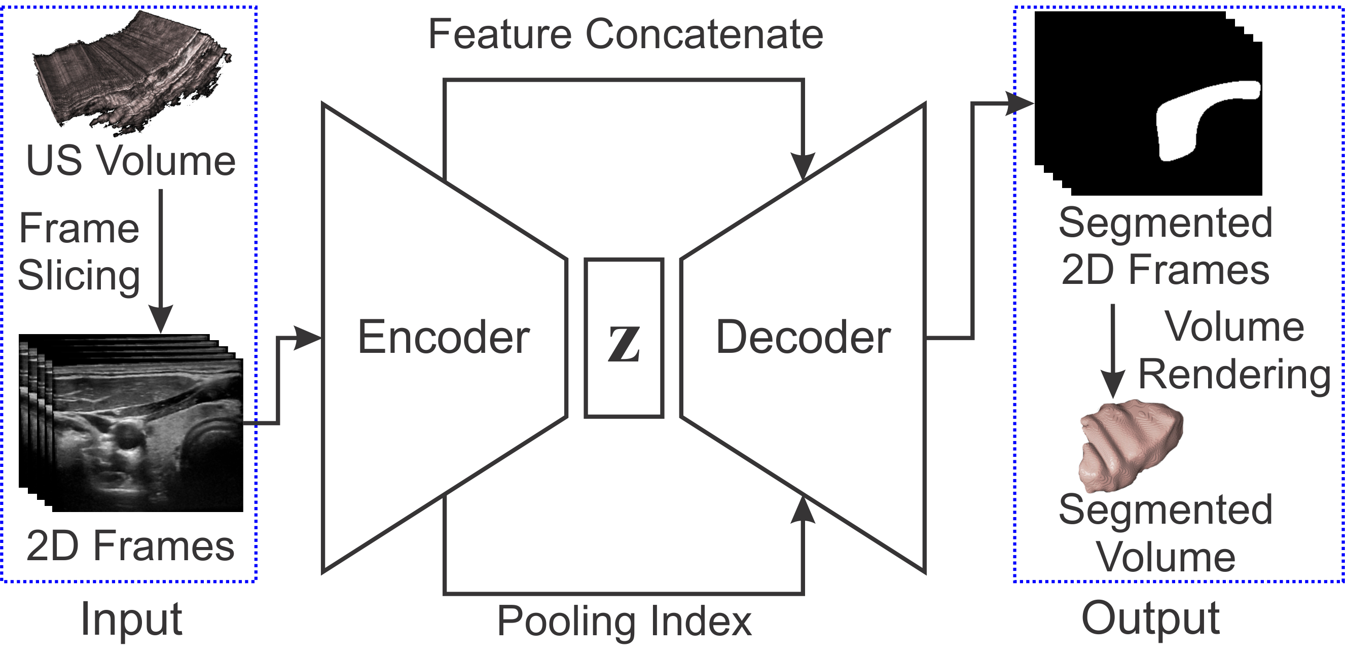
This paper is organized as follows. The existing techniques for ultrasound segmentation are briefly described in Sec. 2. The exposition to the solution is detailed in Sec. 3. The description of data used, experiment performed, results obtained, and their discussions are elucidated in Sec. 4 and the work is concluded in Sec. 5.

2 Prior Art

We present a comprehensive review of the prior art for segmentation in two widely used imaging methods namely (i) inside-out imaging such as with intravascular ultrasound (IVUS) and (ii) outside-in imaging such as for the thyroid.

IVUS Segmentation: Earlier approaches primarily employed non neural network based approaches such as those based on minimization of the probabilistic cost function [7]. This method employed a support vector machine (SVM) trained on the samples of the first frame in a pullback to segment lumen. Balocco et al. [8] reported a comprehensive evaluation of multiple approaches through the 2011 MICCAI workshop, where the methods were tested on a common data. In an earlier work [9] making use of backscattering physics based learning model inspired from  [2], we had proposed an automated algorithm for segmentation of lumen and external elastic laminae which was subsequently extended to use in both outside-in and inside out imaging in  [10]. A fully convolutional network-based architecture, named IVUS-Net [11] is proposed for semantic segmentation of IVUS. Another fully convolutional neural network based architecture based on modified UNet [12] is proposed for semantic segmentation of IVUS and demonstrated only using $40$ MHz data.

Thyroid Segmentation: Prior art included use of level-set active contours model [13] capable of handling segmentation of the thyroid US image. An approach to estimate and classify the thyroid gland in blocks was presented in  [14]. The main advantage of those models are to reduce the effect of intensity inhomogeneity. Later on, feedforward neural networks have been used for segmentation of thyroid [1]. In  [3], three semi-automated approaches based on the level set, graph cut, and feature classification for thyroid segmentation were proposed, while in  [1] authors introduced a multi-organ method for segmenting thyroid gland, carotid artery, muscles, and the trachea.

These algorithms can be grouped as being semi-automatic where they need some basic information about the organ contour, or they employ a prior knowledge about the speckle pattern of the region of interest and the geometric structure of the organ. The algorithms fail to detect the organ boundary, once image quality degrades and contour size decrease. The predominant challenge is that the processing time consumed by these algorithms remains significantly high. Most of the algorithms are not currently usable for 3D volumetric analysis. The motivation of this paper is to resolve the above-mentioned limitations using a deep fully convolution neural network (FCN) for semantic segmentation which we demonstrate here for both inside-out and outside-in ultrasound imaging.

Table 1: Performance evaluation in comparison with prior art. EEL denotes external elastic luminae, JCC denotes Jaccard Coeff. and higher value is better, HD denotes Hausdorff Distance and lower value is better, and PAD denotes Percentage Area Difference and lower value is better.

Methods	JCC		HD		PAD
	Lumen	EEL	Lumen	EEL	Lumen	EEL
P1 - P8 [8]	$0.88\pm 0.05$	$0.91\pm 0.04$	$0.34\pm 0.14$	$0.31\pm 0.12$	$0.06\pm 0.05$	$0.05\pm 0.04$
IVUS-Net [11]	$0.90\pm 0.06$	$0.86\pm 0.11$	$0.26\pm 0.25$	$0.48\pm 0.44$	$-$	$-$
2D SegNet [4]	$0.93\pm 0.05$	$0.89\pm 0.03$	$0.20\pm 0.13$	$0.33\pm 0.10$	$0.07\pm 0.06$	$0.10\pm 0.06$
2D UNet [6]	$0.91\pm 0.06$	$0.88\pm 0.08$	$0.23\pm 0.19$	$0.47\pm 0.31$	$0.10\pm 0.09$	$0.17\pm 0.12$
3D UNet [15]	$0.73\pm 0.13$	$0.76\pm 0.09$	$0.33\pm 0.17$	$0.34\pm 0.14$	$0.21\pm 0.15$	$0.27\pm 0.11$
SUMNet	$\mathbf{0.95}\pm\mathbf{0.03}$	$\mathbf{0.97}\pm\mathbf{0.01}$	$\mathbf{0.17}\pm\mathbf{0.07}$	$\mathbf{0.16}\pm\mathbf{0.09}$	$\mathbf{0.01}\pm\mathbf{0.01}$	$\mathbf{0.01}\pm\mathbf{0.01}$

3 Method

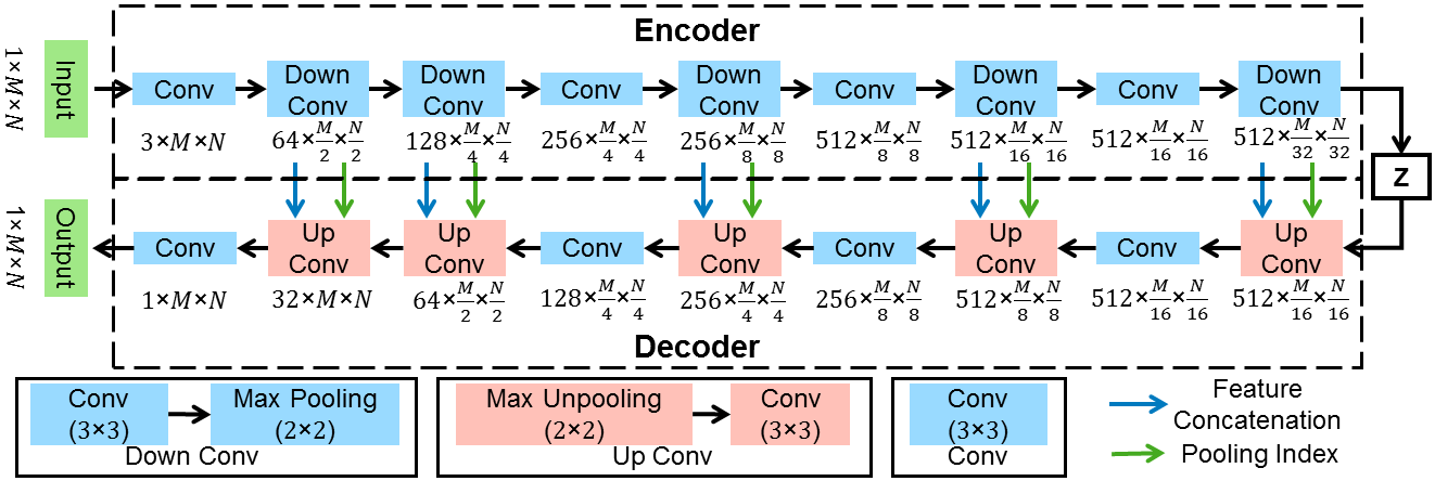
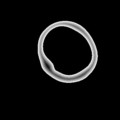
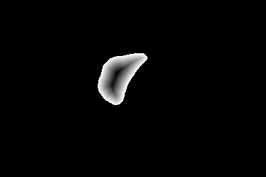
The architecture of the FCN used is illustrated in Fig. 2. It consists of an encoder unit, consisting of convolution and maxpooling layers and a decoder unit consisting of convolution and unpooling layers. The encoder resembles a VGG11 [5] barring the terminal classification layer. Feature maps are downsampled, and the number of features maps increases progressively with layer. The decoder is built to match activation map sizes in layers matched to depth in encoder with use of pooling index transferred for unpooling operation. This improves the boundary segmentation preserving conformity around small structures which is similar to the SegNet [4]. However, max pooling in encoder with a SegNet typically leads to the loss in subtle information related to smaller structures which progressively vanishes across successive depths. To address these limitations, we introduce the activation concatenation concept similar to that used in the UNet [6] which is of relevance to biomedical image segmentation tasks. We have employed ReLU [16] as an activation function in all layer except for the terminal layer of decoder where we have used sigmoid activation function [16] to force the output towards the [0,1] extremity. The network is trained with weighted binary cross-entropy (WCE) [16] loss function. Weights are calculated using a morphological distance transform giving higher weights to the pixels closer to the contour as illustrated for the IVUS in Fig. 3(c) and Fig. 3(j) for thyroid. The idea of using both maxpool indices and concatenating techniques helps in improving the preciseness of localization. The input is a grayscale image, and the first layer of the encoder provides an output with $3$ channel feature map to match input size expected in a VGG11.

4 Experiments, Results and Discussions

A $10$-fold patient wise cross validation has been used with leave-one-patient-out validation.

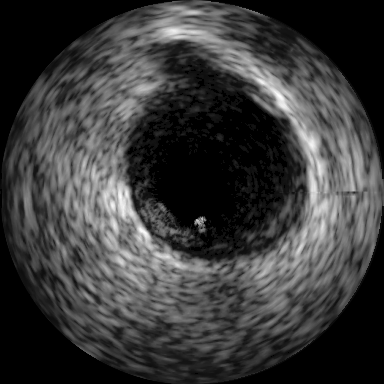
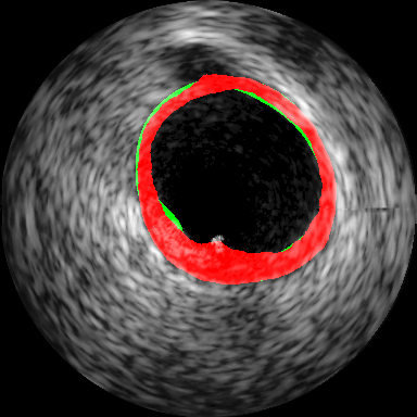
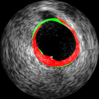
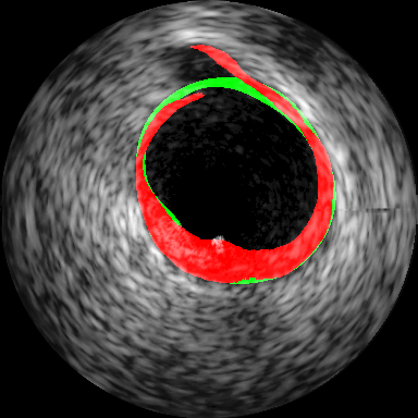
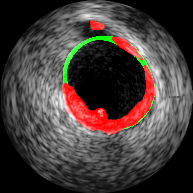
Intravascular Ultrasound Segmentation: We have used IVUS data from the 2011 MICCAI workshop [8] which is composed of $10$ pullbacks of different patients acquired at $20$ MHz (Dataset B). The proposed method is compared with nine different methods, where eight approaches have been reported earlier in [10]. In Table 1, we have included only the best results among the participants (P1-P8) in  [8]. Subsequently 2D visualization of segmented IVUS contours are presented in Fig. 3(d) - (g) and the lumen and external elastic luminae border segmentation in the whole pullback is visualized. The proposed method outperforms the recent related prior art [11] as presented in Table 1.

Table 2: Quantitative analysis and comparison with prior art.

Methods	Sensitivity	Specificity	Dice	PPV
Narayan et al. [1]	$0.96\pm 0.03$	$0.89\pm 0.07$	$0.84\pm 0.05$	$0.81\pm 0.09$
JCR [1]	$0.56\pm 0.07$	$0.93\pm 0.07$	$0.48\pm 0.07$	$0.33\pm 0.06$
Chang et al. [14]	$0.87\pm 0.12$	$0.56\pm 0.32$	$0.51\pm 0.29$	$0.53\pm 0.35$
Garg et al. [1]	$0.47\pm 0.18$	$0.86\pm 0.22$	$0.40\pm 0.14$	$0.27\pm 0.11$
2D SegNet [4]	$0.98\pm 0.07$	$0.84\pm 0.14$	$0.84\pm 0.13$	$0.57\pm 0.26$
2D UNet [6]	$0.98\pm 0.06$	$0.87\pm 0.09$	$0.86\pm 0.09$	$0.63\pm 0.19$
3D UNet [15]	$0.95\pm 0.15$	$0.78\pm 0.30$	$0.67\pm 0.11$	$0.58\pm 0.14$
SUMNet	${0.98}\pm{0.01}$	${0.89}\pm{0.08}$	${0.92}\pm{0.06}$	${0.85}\pm{0.09}$

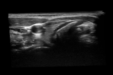
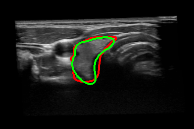
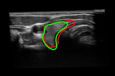
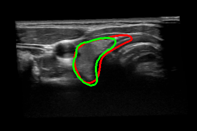
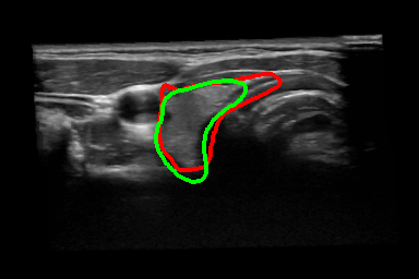
Thyroid Segmentation: The thyroid data used in this experiment has been acquired from a publicly available dataset [3] which includes freehand acquired thyroid US volumes from $16$ healthy human subjects imaged with a $11-16$ MHz probe. The proposed approach is compared with four different algorithms which has been reported by Narayan et. al. [1], (Table. 2). The only limitation in trying to compare commonality is that the dataset used for this comparison is not the same as the dataset used in prior art [1]. 2D visualization of segmentation is shown in Fig. 3(k) - (n) and the thyroid segmentation in the whole volume is visualized . Table 2 shows that our proposed frame work obtain better results than the prior art.

Implementation: We have experimentally trained the network on a PC with Intel Core i5-8600K CPU, 32GB of system RAM, Nvidia Tesla K40c GPU with 12GB DDR5 RAM. The codes are implemented in Python 3.6 and PyTorch 0.4, Nvidia CUDA 9.0 and cuDNN 5.1 on Ubuntu 16.04 LTS OS. The proposed network is trained with a learning rate of $1\times 10^{-3}$, and batch size of 14. Adam optimizer [16] has been used to learn the network weights during training. A CPU platform was used for 3D CNN experiments with large scale memory requirements (Table 3), consists of $2\times$ Intel Xeon 8160 CPU with $12\times 32$GB DDR4 ECC Regd. RAM, Ubuntu 16.04 LTS OS, PyTorch 0.4 on Intel Distribution of Python 3.6 with Intel MKL acceleration.

The proposed network performs better featuring max-unpooling which helps preserve local speckle information, better than transposed convolution where loss of local speckle information due to 4$\times$ padding.

(a) IVUS

(b) Ground truth

(c) Weights

(d) SUMNet

(e) 2D SegNet

(f) 2D UNet

(g) 3D UNet

(h) Thyroid

(i) Ground truth

(j) Weights

(k) SUMNet

(l) 2D SegNet

(m) 2D UNet

(n) 3D UNet

Fig. 3: Weights distribution and 2D visualization of IVUS and thyroid segmentation, where GREEN represents ground truth and RED represents segmentation with the specific method marked in caption.

Table 3: Memory and computation benchmarking of different algorithms for Fig 3(k)- 3(n).

Method	Target	Input size	Batch size	# Batches per epoch	RAM (GB)	Training time per epoch (min)	Inference time per frame (sec)
3D UNet [15]	CPU	$256\times 384\times 384$	1	14	154	29.40	0.145
SUMNet	CPU	$256\times 384$	384	14	148	30.45	0.070
	GPU	$256\times 384$	14	384	9	19.32	0.035
SegNet [4]	CPU	$256\times 384$	384	14	144	26.35	0.055
	GPU	$256\times 384$	14	384	9	15.21	0.031
UNet [6]	CPU	$256\times 384$	384	14	145	27.26	0.068
	GPU	$256\times 384$	14	384	9	18.20	0.032

5 Conclusions

In this paper, we have presented a frame work for automated segmentation of ultrasound volumes using a convolutional neural network. The performance of the proposed architecture is compared with recent prior art, and it is observed that the proposed method outperforms prior art. This network has an advantages to segment boundary region precisely due to the use of WCE as loss function. Activation concatenation concept similar to UNet has been introduced to overcome the critical information loss which happens due to pooling operation and the network is computationally less expensive.

References

- [1] N. S. Narayan, P. Marziliano, J. Kanagalingam, and C. GL. Hobbs, “Speckle patch similarity for echogenicity-based multiorgan segmentation in ultrasound images of the thyroid gland,” IEEE J. Biomed. Health Inform., vol. 21, no. 1, pp. 172–183, 2017.
- [2] D. Sheet, A. Karamalis, A. Eslami, P. Noël, J. Chatterjee, A. K. Ray, A. F. Laine, S. G. Carlier, and A. Navab, N.and Katouzian, “Joint learning of ultrasonic backscattering statistical physics and signal confidence primal for characterizing atherosclerotic plaques using intravascular ultrasound,” Med. Image Anal., vol. 18, no. 1, pp. 103–117, 2014.
- [3] T. Wunderling, B. Golla, P. Poudel, C. Arens, M. Friebe, and C. Hansen, “Comparison of thyroid segmentation techniques for 3d ultrasound,” in Proc. Med. Imaging Image Process., 2017, vol. 10133, p. 1013317.
- [4] V. Badrinarayanan, A. Kendall, and R. Cipolla, “Segnet: A deep convolutional encoder-decoder architecture for image segmentation,” IEEE Trans. Patt. Anal. Mach. Intell., vol. 39, no. 12, pp. 2481–2495, 2017.
- [5] K. Simonyan and A. Zisserman, “Very deep convolutional networks for large-scale image recognition,” Proc. Int. Conf. Learn. Represent., 2015.
- [6] O. Ronneberger, P. Fischer, and T. Brox, “U-net: Convolutional networks for biomedical image segmentation,” in Proc. Int. Conf. Med. Image comput. Comput. Assist. Interv., 2015, pp. 234–241.
- [7] E. G. Mendizabal-Ruiz, M. Rivera, and I. A. Kakadiaris, “Segmentation of the luminal border in intravascular ultrasound b-mode images using a probabilistic approach,” Med. Image Anal., vol. 17, no. 6, pp. 649–670, 2013.
- [8] S. Balocco, C. Gatta, F. Ciompi, A. Wahle, P. Radeva, S. Carlier, G. Unal, E. Sanidas, J. Mauri, X. Carillo, et al., “Standardized evaluation methodology and reference database for evaluating ivus image segmentation,” Comput. Med. Imaging Graph., vol. 38, no. 2, pp. 70–90, 2014.
- [9] D. China, P. Mitra, and D. Sheet, “On the fly segmentation of intravascular ultrasound images powered by learning of backscattering physics,” in Classification in BioApps, pp. 351–380. 2018.
- [10] D. China, A. Illanes, P. Poudel, M. Friebe, P. Mitra, and D. Sheet, “Anatomical structure segmentation in ultrasound volumes using cross frame belief propagating iterative random walks.,” IEEE J. Biomed. Health Inform., 2018.
- [11] J. Yang, L. Tong, M. Faraji, and A. Basu, “Ivus-net: An intravascular ultrasound segmentation network,” arXiv preprint arXiv:1806.03583, 2018.
- [12] S. Kim, Y. Jang, B. Jeon, Y. Hong, H. Shim, and H. Chang, “Fully automatic segmentation of coronary arteries based on deep neural network in intravascular ultrasound images,” in Intravascular Imaging, Comp. Assist. Stenting, Large-Scale Anno., Biomed. Data, Expert Label Syn., pp. 161–168. 2018.
- [13] M. A. Savelonas, D. K. Iakovidis, I. Legakis, and D. Maroulis, “Active contours guided by echogenicity and texture for delineation of thyroid nodules in ultrasound images,” IEEE Trans. Inf. Technol. Biomed., vol. 13, no. 4, pp. 519–527, 2009.
- [14] C. Chang, Y. Lei, C. Tseng, and S. Shih, “Thyroid segmentation and volume estimation in ultrasound images,” IEEE Trans. Biomed. Engg., vol. 57, no. 6, pp. 1348–1357, 2010.
- [15] Ö. Çiçek, A. Abdulkadir, S. S. Lienkamp, T. Brox, and O. Ronneberger, “3d u-net: learning dense volumetric segmentation from sparse annotation,” in Proc. Int. Conf. Med. Image Comput. Comput. Assist. Interv., 2016, pp. 424–432.
- [16] I. Goodfellow, Y. Bengio, A. Courville, and Y. Bengio, Deep learning, vol. 1, 2016.