CASCLIK: CasADi-Based Closed-Loop Inverse Kinematics

Abstract

A Python module for rapid prototyping of constraint-based closed-loop inverse kinematics controllers is presented. The module allows for combining multiple tasks that are resolved with a quadratic, nonlinear, or model predictive optimization-based approach, or a set-based task-priority inverse kinematics approach. The optimization-based approaches are described in relation to the set-based task approach, and a novel multidimensional “in tangent cone” function is presented for set-based tasks. A ROS component is provided, and the controllers are tested with matching a pose using either transformation matrices or dual quaternions, trajectory tracking while remaining in a bounded workspace, maximizing manipulability during a tracking task, tracking an input marker’s position, and force compliance.

I Introduction

Robots perform tasks that involve interacting and moving objects in Cartesian space by moving joints and motors. Finding control setpoints in terms of the joint coordinates such that the robot can achieve the desired task requires solving the inverse kinematics problem. Inverse kinematics is fundamental to all robots, and occurs in everything from humanoid service robots to 3D printers, surgical robots to autonomous vehicles. In this article we present CASCLIK, a Python module for rapid prototyping of closed-loop inverse kinematics controllers for realizing multiple constraint-based tasks.

Closed-loop inverse kinematics involves defining a feedback controller for achieving the desired task. In [1], Sciavicco et al. present a closed-loop inverse kinematic approach where joint speed setpoints minimize the distance to a given end-effector pose. The distance errors have a guaranteed convergence characteristics. The controller works by inverting the differential kinematics and defines a continuous motion control of the robot.

The task function approach by Samson et al. [2] describes a robotic task as defined by an arbitrary output function and a control objective. The output function is a mapping from the joint states and time to an output space. Samson formulates the task such that the control objective is to bring the output function to zero. The task function approach generalizes to a large class of tasks as the output function may go from any robot states to any positions or orientations defined relative the robot or world frame.

The constraint-based task specification approach of De Schutter et al. [3] describes procedures for designing tasks with complex sensor-based robot systems and geometric uncertainties. Constraint-based task specification uses variables termed feature variables to describe position of geometric and task related features that are useful for the task. A key aspect of constraint-based task specification is to allow for feature variables.

A robot is redundant with respect to its task when it has more degrees of freedom than there are dimensions in the output function of the task. This allows one to utilize the free degrees of freedom to achieve tasks simultaneously. A common approach to handling redundancy involves inverting the differential kinematics using a pseudo-inverse. The pseudo-inverse often introduces a null-space within which additional tasks can be achieved. To the author’s knowledge, the earliest article combining multiple tasks in this manner is by Hanafusa et al. [4] where a 7 degrees-of-freedom robot tracks a trajectory and avoids an obstacle. This is achieved by placing the lower priority tracking task in the null-space of the higher priority obstacle avoidance task. Chiaverini et al. shows in [5] that multiple tasks can be combined in a singularity robust way. Any framework that supports closed-loop inverse kinematics using task specification should allow for multiple tasks. The state of the art presents two approaches to multiple tasks, strict prioritization with null-space based approaches such as the set-based singularity robust task-priority inverse kinematics framework [6] and optimization-based prioritization which lacks strict priority but allows prioritization through the cost function in an optimization problem [7].

Calculating the Jacobians involved in closed-loop inverse kinematics has been a complicated process requiring explicit knowledge of the underlying representation used in the tasks. Modern algorithmic differentiation systems such as CasADi [8] simplify this process, allowing us to generate compiled functions of complicated Jacobians. CasADi uses a symbolic framework for performing algorithmic differentiation on expression graphs to construct Jacobians. CasADi provides methods for formulating linear, quadratic, and nonlinear problems that can be solved with e.g. QPOASES [9] and IPOPT [10]. CASCLIK translates a set of tasks to optimal problems of a form that CasADi can solve. This allows the user to test constraint-based programming with any of the available optimizers in CasADi with the different controller formulations presented in this article. The purpose of CASCLIK is to facilitate rapid prototyping of constraint-based control of robot systems.

The architecture of CASCLIK is inspired by eTaSL/eTC [7] by Aertbeliën et al., which is a more mature task specification language and controller. A core principle of the architecture of eTaSL/eTC is to separate the low-level robot controller, numerical solver, and the task specification. Tasks are robot-agnostic and transferrable to any robot system with known forward kinematics. The power of constraint-based task specification and control has allowed the creation of a system architecture capable of exploiting CAD knowledge for assembly [11], for which this work may present alternative controller formulations of interest. Robot-agnostic task specification enables execution of the same task with different robot platforms, which also allows for easier delegation of tasks to the appropriate robots, and transferral of skills from one robot system to another.

CASCLIK is a CasADi-based Python module for testing closed-loop inverse kinematics controllers. The module focuses on being cross-platform and defers to CasADi for the symbolic backend and optimization. The purpose of this module is to explore alternative controller and constraint formulations that utilize the same general structure as eTaSL/eTC. It considers nonlinear and model predictive formulations which are less real-time applicable, in an attempt to investigate aspects that may later be implemented into more industrially relevant frameworks. As it uses CasADi for optimization, CASCLIK utilizes the development efforts of the CasADi community to enable a variety of solvers.

The article is divided into six sections. The first section introduces relevant concepts such as closed-loop inverse kinematics, task function approach, algorithmic differentiation, and presents modern related research. The second section describes the theory involved in CASCLIK. The third section gives a brief description of the implementation. The fourth section gives example applications of CASCLIK and preliminary studies. The fifth and sixth section is the discussion and conclusion.

The main contributions of the article are:

• A nonlinear programming formulation of the constraint-based closed-loop inverse kinematics task controller,

• a model predictive formulation of the constraint-based closed-loop inverse kinematics task controller,

• a general implementation of the set-based singularity robust multiple task-priority inverse kinematics framework of [6],

• a novel multidimensional in tangent cone function for the set-based singularity robust multiple task-priority inverse kinematics framework,

I-A Related Research

When considering fundamental robotics problems such as inverse kinematics, there are innumerable important references. To limit the scope we focus on related modern frameworks.

Stack-of-Tasks [12, 13] is a C++ software development kit for real-time motion control of redundant robots. Tasks and robots are defined using dynamic graphs that allow for caching results in functions for fast evaluation. The system allows for equality and set tasks by activating and deactivating control of the set tasks. The framework allows for joint torque level control of the robot. Stack-of-tasks also supports a hierarchical quadratic programming formulation [14]. It is open-source, includes tools for integration with ROS, and is limited to Unix platforms.

iTaSC [15, 16] is a software framework for constraint-based task specification and execution. It presents a modular design for task specification, scenegraph representation, and solver. The software framework is a part of the OROCOS project, and uses OROCOS RTT [17, 18] to control robots.

The previously mentioned eTaSL/eTC [7] is a successor to iTaSC, and is a C++/LUA constraint-based task specification and control framework. Expressions are formulated using expressiongraphs [19], a symbolic framework that uses OROCOS KDL definitions [20] for frames and rotations. Arbitrary symbolic expressions are used in constraints to form a task specification. The architecture of eTaSL/eTC is modular, allowing one to define new controllers for a task specification and new solvers if they have a C++ interface. It currently supports QPOASES and the hierarchical quadratic programming solver of Stack-of-Tasks. eTaSL/eTC includes a Python interface for rapid prototyping and an OROCOS RTT [17, 18] component for real-time control of robots using OROCOS. eTaSL/eTC is open-source and is currently limited to Linux platforms.

Other advanced constraint-based approaches include the task level robot programming framework of Somani et al.[21], that supports an optimization based solver, and an analytical solver [22]. The software focuses on semantic process description and CAD level tasks and constraints [23]. The CAD level constraints have composition rules, allowing for a reduction of the space of possible control setpoints. The reduced space is used to formulate the analytical solver. To the author’s knowledge, the software is not open-source.

The set-based singularity robust multiple task-priority inverse kinematics controller [6] is a task controller that uses the augmented null-space projection operator [24] and activation or deactivation of null-spaces to implement set tasks. This controller forms the null-space approach in CASCLIK and this article extends the approach with support for multidimensional set constraints.

II Theory

In this section we present the underlying theory used in CASCLIK. We present the variables and output function involved, the available control objectives one can define, the convexity of the constraints in optimization based controllers, and their effect in the null-space projection based controller. Then we present the four different controllers available: the quadratic, nonlinear, and model predictive optimization-based approaches, and the null-space projection approach. The quadratic programming approach is based on eTaSL/eTC [7] and the null-space approach is based on the set-based singularity robust task-priority inverse kinematics controller [6].

II-A Variables and Output Function

CASCLIK currently supports four different variable types:

• $t$, time,

• $\bm{q}(t)\in\mathbb{R}^{n_{q}}$, robot variable (e.g. joint angles),

• $\bm{x}(t)\in\mathbb{R}^{n_{x}}$, virtual variable (e.g. path-timing),

• $\bm{y}(t)\in\mathbb{R}^{n_{y}}$, input variables (e.g. sensor values).

Time and robot variables are self-explanatory. Virtual variables are similar to the feature variables of eTaSL/eTC or iTaSC, but the term feature implies a relation to geometric aspects of the task. We describe these as virtual variables as they are variables maintained by the computer, and not necessarily linked to any features of the objects involved. This is merely a semantic choice. Virtual variables simplify task specification and are present in cases such as path-following. Input variables are variables for which we have no information about the derivative behavior.

The output function is a function:

$$\bm{e}(t,\bm{q},\bm{x},\bm{y})\in\mathbb{R}^{n_{e}},$$ (1)

where $n_{e}\leq n_{q}+n_{x}$ and $t$, $\bm{x}$ and $\bm{y}$ are optional. In CASCLIK we assume no knowledge of the underlying geometry involved when evaluating the partial derivatives of the output function. This differs from most other closed-loop inverse kinematics frameworks where the representation is used when evaluating the derivative of transformation matrices and orientations. This is a design choice to make the library as general as possible and allows us to inspect the behavior with different representations. This may require more from the task programmer as the behavior of the robot may differ depending on the formulation of the output function.

Assumption 1 (Velocity Control).

The robot system is equipped with a sufficiently fast velocity controller giving $\dot{\bm{q}}(t)=\dot{\bm{q}}_{des}(t)$ where $\dot{\bm{q}}_{des}$ is the designed control setpoint. The velocity controller controls all robot state velocities.

Samson et al. [2] describe how the first industrial robots had velocity-controlled electrical motors, leading to the joint velocity becoming the “true control variable” for robot systems in the control literature. Assumption 1 stems from this time and has been a common robotics assumption since.

II-B Constraints

We use a formulation of robotic tasks similar to Samson et al.[2]: a task is defined by an output function and a control objective. Samson et al. defines the control objective as a regulation problem where a task is performed perfectly during $[t_{0},t_{f}]$ if

$$\bm{e}(t,\bm{q},\bm{x},\bm{y})=0$$ (2)

for all $t\in[t_{0},t_{f}]$. This is achieved by designing a controller such that the output function converges to zero.

Similar to eTaSL, we refer to the control objective as a type of constraint. CASCLIK specifies four types of constraints:

• equality constraints,

  $$\bm{e}(t,\bm{q},\bm{x},\bm{y})=0,$$ (3)

• set constraints,

  $$\bm{e}_{l}(t,\bm{q},\bm{x},\bm{y})\leq\bm{e}(t,\bm{q},\bm{x},\bm{y})\leq\bm{e}_{u}(t,\bm{q},\bm{x},\bm{y}),$$ (4)

• velocity equality constraints,

  $$\dot{\bm{e}}(t,\bm{q},\bm{x},\bm{y})=\dot{\bm{e}}_{d}(t,\bm{q},\bm{x},\bm{y}),$$ (5)

• and velocity set constraints,

  $$\dot{\bm{e}}_{l}(t,\bm{q},\bm{x},\bm{y})\leq\dot{\bm{e}}(t,\bm{q},\bm{x},\bm{y})\leq\dot{\bm{e}}_{u}(t,\bm{q},\bm{x},\bm{y}).$$ (6)

where subscript $l$ and $u$ refer to the lower and upper bounds, and subscript $d$ refers to a desired derivative of the output function. The control objectives of the tasks are achieved perfectly if the equations hold during $t\in[t_{0},t_{f}]$.

As the control objectives both include equality (converging to zero), and set constraints (converging to or remaining in a set), and set constraints can have different upper and lower bounds, we cannot use the regulation problem formulation of Samson et al. We rely on linearization of the time-derivative of the output functions to achieve the control objectives.

Assumption 2 (Linearization).

The partial derivatives $\frac{\partial\bm{e}}{\partial t},\frac{\partial\bm{e}}{\partial\bm{q}}$ and $\frac{\partial\bm{e}}{\partial\bm{x}}$ (commonly called the task Jacobian) can be considered constant with respect to the control duration. That is:

$$\frac{\partial\bm{e}}{\partial t}(\tau)+ \frac{\partial\bm{e}}{\partial\bm{q}}(\tau)\dot{\bm{q}}(t_{n})+\frac{\partial\bm{e}}{\partial\bm{x}}(\tau)\dot{\bm{x}}(t_{n})\approx$$

$$\frac{\partial\bm{e}}{\partial t}(t_{n})+\frac{\partial\bm{e}}{\partial\bm{q}}(t_{n})\dot{\bm{q}}(t_{n})+\frac{\partial\bm{e}}{\partial\bm{x}}(t_{n})\dot{\bm{x}}(t_{n})$$ (7)

for $t_{n}\leq\tau\leq t_{n}+\Delta_{t}$ where $t_{n}$ is a sampling point and $\Delta_{t}$ is the duration of the control step.

The linearization assumption is often used in closed-loop inverse kinematics frameworks without explicitly stating it as an assumption. The linearization assumption does not always hold, and for long control steps or rapidly moving trajectories a tracking error may occur [25].

Defining a controller for a set of tasks is finding $(\dot{\bm{q}},\dot{\bm{x}})$ such that we achieve the tasks. For the optimization-based controller approaches we do this by imposing constraints on the optimization problem, and for the null-space approach we do this by both null-space projection and inversion of the differential kinematics.

II-B1 Equality Constraints

Taking the time-derivative of the output function, we get:

$$\dot{\bm{e}}=\frac{\partial\bm{e}}{\partial t}+\frac{\partial\bm{e}}{\partial\bm{q}}\dot{\bm{q}}+\frac{\partial\bm{e}}{\partial\bm{x}}\dot{\bm{x}}$$ (8)

where the best guess for the derivatives of $\bm{y}$ is zero. An equality constraint forms a regulation problem, which is achieved by ensuring that:

$$\dot{\bm{e}}=\frac{\partial\bm{e}}{\partial t}+\frac{\partial\bm{e}}{\partial\bm{q}}\dot{\bm{q}}+\frac{\partial\bm{e}}{\partial\bm{x}}\dot{\bm{x}}=-\bm{K}(t,\bm{q},\bm{x},\bm{y})\bm{e}(t,\bm{q},\bm{x},\bm{y})$$ (9)

for which exponential convergence to zero is guaranteed if (9) is upheld and $\bm{K}$ is positive definite. $\bm{K}$ is a user-defined function, and its dependent variables will be omitted for brevity in the rest of the paper.

Velocity equality constraints are included to allow for velocity following, but do not guarantee convergence:

$$\dot{\bm{e}}=\frac{\partial\bm{e}}{\partial t}+\frac{\partial\bm{e}}{\partial\bm{q}}\dot{\bm{q}}+\frac{\partial\bm{e}}{\partial\bm{x}}\dot{\bm{x}}=\dot{\bm{e}}_{d}(t,\bm{q},\bm{x},\bm{y}),$$ (10)

where the right hand side is the desired constraint velocity. This is to accommodate control situations for which the desired output function derivative is easy to define, but its integral is not. Because we rely on Assumption 1 and Assumption 2, the lack of convergence of velocity constraints is not considered in this article.

By using the Moore-Penrose pseudo-inverse (superscript $\dagger$) we get (9) and (10) on a form that fits with the null-space projection approach. For equality constraints it becomes:

$$\begin{bmatrix}\dot{\bm{q}}\\ \dot{\bm{x}}\end{bmatrix}=-{\left(\begin{bmatrix}\frac{\partial\bm{e}}{\partial\bm{q}}&\frac{\partial\bm{e}}{\partial\bm{x}}\end{bmatrix}\right)}^{\dagger}\left(\bm{K}\bm{e}+\frac{\partial\bm{e}}{\partial t}\right).$$ (11)

Similarly for the velocity equality constraint we have:

$$\begin{bmatrix}\dot{\bm{q}}\\ \dot{\bm{x}}\end{bmatrix}={\left(\begin{bmatrix}\frac{\partial\bm{e}}{\partial\bm{q}}&\frac{\partial\bm{e}}{\partial\bm{x}}\end{bmatrix}\right)}^{\dagger}\left(\dot{\bm{e}}_{d}-\frac{\partial\bm{e}}{\partial t}\right).$$ (12)

II-B2 Set Constraints

Set constraints are different in optimization approaches and the null-space projection approach. In optimization based controllers we enable exponential convergence to the set by defining the constraint as:

$$\bm{K}(\bm{e}-\bm{e}_{l})\leq\frac{\partial\bm{e}}{\partial t}+ \frac{\partial\bm{e}}{\partial\bm{q}}\dot{\bm{q}}+\frac{\partial\bm{e}}{\partial\bm{x}}\dot{\bm{x}}\leq\bm{K}(\bm{e}-\bm{e}_{u})$$ (13)

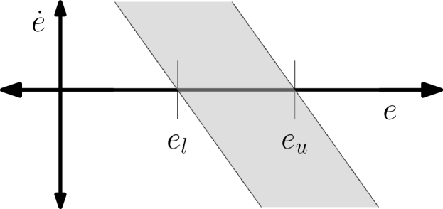
where the gain is defined as previously. Fig.1 visualizes how (13) leads to convergence. When approaching a limit from inside the constraint, the maximum of $\dot{\bm{e}}$ will gradually be reduced, which causes an exponential decay when approaching a constraint limit.

Figure 1: Visualization of set constraint convergence in one dimension. $\dot{\bm{q}}$ and $\dot{\bm{x}}$ must be chosen such that $\dot{e}$ remains in the gray area. As this results in requiring $\dot{e}$ to be positive when $e<e_{l}$ and negative when $e>e_{u}$, we will converge to $e_{l}\leq e\leq e_{u}$. The slope of the lines are defined by $K$.

Similar to the velocity equality constraints, velocity set constraints do not ensure convergence and are defined as:

$$\dot{\bm{e}}_{l}(t,\bm{q},\bm{x},\bm{y})\leq\frac{\partial\bm{e}}{\partial t}+\frac{\partial\bm{e}}{\partial\bm{q}}\dot{\bm{q}}+\frac{\partial\bm{e}}{\partial\bm{x}}\dot{\bm{x}}\leq\dot{\bm{e}}_{u}(t,\bm{q},\bm{x},\bm{y})$$ (14)

which can be visualized as horizontal lines in Fig.1.

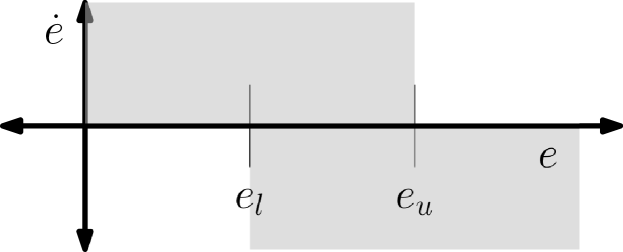
Set constraints in the null-space approach are handled using null-space projection and the in tangent cone function (Algorithm 1 in [6]). The method states that if the desired $(\dot{\bm{q}},\dot{\bm{x}})$ ensures that the output function remains in the set, by asking whether the $(e,\dot{e})$ pair is in the extended tangent cone, then the set constraint is not active. If the desired robot state velocity is not in the extended tangent cone then the set constraint is active and lower priority tasks are modified by the null-space projection operator of the active set constraint. The choice of $(e,\dot{e})$ pairs that do not cause an activation of the set constraint is visualized in Fig.2.

Figure 2: Visualization of when in tangent cone evaluates to true for a one-dimensional output function. For any $(e,\dot{e})$ not in the gray area, the set constraint becomes active and lower level tasks are projected into the null-space of the set constraint.

In [25] it was noted that formulating multidimensional tracking tasks as one dimensional tasks of differing priorities may lead to unexpected tracking errors. The in tangent cone function of Moe et al. [6] assumes one-dimensional output functions. CASCLIK addresses this by implementing a multidimensional version which allows for using multidimensional output functions with set constraints. The algorithm is given in Alg.1. If at a time we are at $\bm{e}$ then the vector $\bm{d}$ describes the normal vector to the closest point that is in the set. This allows us to identify when $\dot{\bm{e}}$ points inwards. The signs of $\bm{e}-\bm{e}_{l}$ and $\bm{e}-\bm{e}_{u}$ are equal when the closest point inside the set is on the corners of a set, allowing us to identify the corners as special cases.

Algorithm 1 Multidimensional in tangent cone

0:  $t,\bm{q},\bm{x},\bm{y},\dot{\bm{q}},\dot{\bm{x}}$

1:  $\bm{d}\leftarrow\textrm{sign}(\bm{e}-\bm{e}_{l})+\textrm{sign}(\bm{e}-\bm{e}_{u})$

2:  $\textrm{in\_crnr}\leftarrow\textrm{sign}(\bm{e}-\bm{e}_{l})==\textrm{sign}(\bm{e}-\bm{e}_{u})$

3:  if $\bm{e}_{l}(t,\bm{q},\bm{x},\bm{y})\leq\bm{e}(t,\bm{q},\bm{x},\bm{y})\leq\bm{e}_{u}(t,\bm{q},\bm{x},\bm{y})$ then

4:     return  True

5:  else if in_crnr and $|\bm{-d}\cdot\dot{\bm{e}}|<\left\lVert\bm{d}\right\rVert\left\lVert\dot{\bm{e}}\right\rVert\cos(45^{\circ})$ then

6:     return  True

7:  else if not in_crnr and $\bm{d}\cdot\dot{\bm{e}}<0$ then

8:     return  True

9:  else

10:     return  False

11:  end if

The multidimensional in tangent cone function assumes that corners can be approximated with a $45^{\circ}$ cone situated at the corner. This is an approximation that may falsely report that we are not in the extended tangent cone for $\textrm{dim}(\bm{e})>2$, e.g. when the desired $\dot{\bm{e}}$ points along an edge of the set constraint.

Velocity set constraints are not currently defined in the task-priority inverse kinematics framework, and are therefore not included in the null-space projection approach.

II-B3 Convexity of Desired Control Input Space

For the optimization-based approaches, the task constraints form constraints in the optimization problem. The derivative of the output function is an affine function with respect to the desired control input $\dot{\bm{q}}$ and $\dot{\bm{x}}$. For the different constraint types, the space of desired control inputs are:

$$\mathcal{D}(\bm{e},eq)= \left\{\dot{\bm{q}},\dot{\bm{x}}\bigg{|}\frac{\partial\bm{e}}{\partial t}+\frac{\partial\bm{e}}{\partial\bm{q}}\dot{\bm{q}}+\frac{\partial\bm{e}}{\partial\bm{x}}\dot{\bm{x}}=-\bm{K}\bm{e}\right\}$$ (15)

$$\mathcal{D}(\bm{e},vel.eq)= \left\{\dot{\bm{q}},\dot{\bm{x}}\bigg{|}\frac{\partial\bm{e}}{\partial t}+\frac{\partial\bm{e}}{\partial\bm{q}}\dot{\bm{q}}+\frac{\partial\bm{e}}{\partial\bm{x}}\dot{\bm{x}}=\dot{\bm{e}}_{d}\right\}$$ (16)

$$\mathcal{D}(\bm{e},set)=$$

$$\bigg{\{}\dot{\bm{q}},\dot{\bm{x}}\bigg{|}\frac{\partial\bm{e}}{\partial t}+\frac{\partial\bm{e}}{\partial\bm{q}}\dot{\bm{q}} +\frac{\partial\bm{e}}{\partial\bm{x}}\dot{\bm{x}}\in[\bm{K}(\bm{e}-\bm{e}_{l}),\bm{K}(\bm{e}-\bm{e}_{u})]\bigg{\}}$$ (17)

$$\mathcal{D}(\bm{e},vel.set)= \left\{\dot{\bm{q}},\dot{\bm{x}}\bigg{|}\frac{\partial\bm{e}}{\partial t}+\frac{\partial\bm{e}}{\partial\bm{q}}\dot{\bm{q}}+\frac{\partial\bm{e}}{\partial\bm{x}}\dot{\bm{x}}\in[\dot{\bm{e}}_{l},\dot{\bm{e}}_{u}]\right\}.$$ (18)

At any particular time instance $t,\bm{q},\bm{x}$ and $\bm{y}$ are constant, making $\dot{\bm{e}}$ an affine transformation with respect to $\dot{\bm{q}}$ and $\dot{\bm{x}}$. From [26] we know that the inverse image of an affine function on a convex set is convex, which makes $\mathcal{D}$ convex. The set of possible choices of $(\dot{\bm{q}},\dot{\bm{x}})$ with multiple tasks is

$$\bm{\mathcal{S}}(t,\bm{q},\bm{x},\bm{y})=\bigcap_{i=1}^{n_{c}}\mathcal{D}(\bm{e}_{i},c_{i})(t,\bm{q},\bm{x},\bm{y}),$$ (19)

where we have $n_{c}$ tasks, each with an output function $\bm{e}_{i}$ and a control objective $c_{i}\in\{eq.,vel.eq.,set,vel.set\}$. As the intersection of convex sets is convex, combining tasks maintains convexity of the set of possible control variables. This convexity hinges on the derivative of the output function being affine with respect to the control variables. Thus the convexity argument does not hold for the model predictive approach where $\bm{q}$ and $\bm{x}$ are predicted variables for the predicted constraints.

Tasks are incompatible if $\mathcal{S}=\emptyset$ (e.g. first task is to remain in a box, second task is to track a reference that leaves the box). We can easily see that adding a slack variable term $\bm{\epsilon}$ to $\dot{\bm{e}}$ reinstates the convexity with respect to the variables $(\dot{\bm{q}},\dot{\bm{x}},\bm{\epsilon})$ for the non-predictive approaches.

II-B4 Null-Space Projection

Given an output function $\bm{e}_{i}$, we define the null-space projection operator of the task as:

$$\bm{N}_{i}=\bm{I}_{n_{q}+n_{x}}-{\begin{bmatrix}\frac{\partial\bm{e}_{i}}{\partial\bm{q}},\frac{\partial\bm{e}_{i}}{\partial\bm{x}}\end{bmatrix}}^{\dagger}\begin{bmatrix}\frac{\partial\bm{e}_{i}}{\partial\bm{q}},\frac{\partial\bm{e}_{i}}{\partial\bm{x}}\end{bmatrix}$$ (20)

such that $\bm{N}_{i}\bm{v}=0$ if $\bm{v}$ is a vector that extends only into the space of the task. For multiple tasks, the null-space of all the tasks combined uses the augmented inverse-based projection of [24]:

$$\bm{N}_{i,i+1,\dots}=\bm{I}_{n_{q}+n_{x}}-{\begin{bmatrix}\frac{\partial\bm{e}_{i}}{\partial\bm{q}},\frac{\partial\bm{e}_{i}}{\partial\bm{x}}\\ \frac{\partial\bm{e}_{i+1}}{\partial\bm{q}},\frac{\partial\bm{e}_{i+1}}{\partial\bm{x}}\\ \vdots\end{bmatrix}}^{\dagger}\begin{bmatrix}\frac{\partial\bm{e}_{i}}{\partial\bm{q}},\frac{\partial\bm{e}_{i}}{\partial\bm{x}}\\ \frac{\partial\bm{e}_{i+1}}{\partial\bm{q}},\frac{\partial\bm{e}_{i+1}}{\partial\bm{x}}\\ \vdots\end{bmatrix}$$ (21)

With multidimensional set constraints the null-space should only consider directions in which the output function violates the set constraints. For each set constraint we define a diagonal activation matrix $\bm{S}_{i}\in\mathbb{R}^{n_{e_{i}}\times{n_{e_{i}}}}$ with diagonal elements:

$$s_{i,j}=\left\{\begin{matrix}1,&e_{i,j}<e_{l,i,j}\text{ or }e_{i,j}>e_{u,i,j}\\ 0,&\text{else}\end{matrix}\right.$$ (22)

where subscript $i,j$ refers to $j$th element of the $i$th output function, upper bound, or lower bound. With the activation matrix, the augmented inverse-based projection becomes:

$$\bm{N}_{i,i+1,\dots}=\bm{I}_{n_{q}+n_{x}}-{\begin{bmatrix}\frac{\partial\bm{e}_{i}}{\partial\bm{q}},\frac{\partial\bm{e}_{i}}{\partial\bm{x}}\\ \frac{\partial\bm{e}_{i+1}}{\partial\bm{q}},\frac{\partial\bm{e}_{i+1}}{\partial\bm{x}}\\ \vdots\end{bmatrix}}^{\dagger}\begin{bmatrix}\bm{J}_{A,i}\\ \bm{J}_{A,i+1}\\ \vdots\end{bmatrix}$$ (23)

where

$$\bm{J}_{A,i}=\left\{\begin{matrix}[\frac{\partial\bm{e}_{i}}{\partial\bm{q}},\frac{\partial\bm{e}_{i}}{\partial\bm{x}}],&\text{if equality constraint}\\ \bm{S}_{i}[\frac{\partial\bm{e}_{i}}{\partial\bm{q}},\frac{\partial\bm{e}_{i}}{\partial\bm{x}}],&\text{if set constraint}.\end{matrix}\right.$$ (24)

II-C Quadratic Programming Approach

The quadratic programming (QP) approach is a reactive control that formulates a QP problem based on the current sensor information. At time $t=t_{k}$, we know $\bm{q}(t_{k})$,$\bm{x}(t_{k})$, and $\bm{y}(t)$. $\dot{\bm{q}}_{k}$ is a setpoint sent to the robot system and $\dot{\bm{x}}_{k}$ is used to obtain $\bm{x}_{k+1}$. The optimization problem is:

$$\min_{\dot{\bm{q}}_{k},\dot{\bm{x}}_{k},\bm{\epsilon}}\quad c\dot{\bm{q}}_{k}^{T}\bm{W}_{\dot{\bm{q}}}\dot{\bm{q}}_{k}+c\dot{\bm{x}}_{k}^{T}\bm{W}_{\dot{\bm{x}}}\dot{\bm{x}}_{k}+(1+c)\bm{\epsilon}^{T}W_{\bm{\epsilon}}\bm{\epsilon}$$ (25a)

$$s.t.:\quad$$

$$(\dot{\bm{q}}_{k},\dot{\bm{x}}_{k})\in\mathcal{S}(t_{k},\bm{q}(t_{k}),\bm{x}(t_{k}),\bm{y}(t_{k}),\bm{\epsilon})$$ (25b)

where $\mathcal{S}$ is the set of all $(\dot{\bm{q}}_{k},\dot{\bm{x}}_{k})$ such that:

$$\frac{\partial\bm{e}_{i}}{\partial t}+\frac{\partial\bm{e}_{i}}{\partial\bm{q}}\dot{\bm{q}}_{k}+\frac{\partial\bm{e}_{i}}{\partial\bm{x}}\dot{\bm{x}}_{k}=-\bm{K}_{i}\bm{e}_{i}+\bm{\epsilon}_{i}$$ (26)

$$\bm{K}_{j}(\bm{e}_{j}-\bm{e}_{l,j})\leq\frac{\partial\bm{e}_{j}}{\partial t}+\frac{\partial\bm{e}_{j}}{\partial\bm{q}}\dot{\bm{q}}_{k}+\frac{\partial\bm{e}_{j}}{\partial\bm{x}}\dot{\bm{x}}_{k}+\bm{\epsilon}_{j}$$ (27)

$$` \frac{\partial\bm{e}_{j}}{\partial t}+\frac{\partial\bm{e}_{j}}{\partial\bm{q}}\dot{\bm{q}}_{k}+\frac{\partial\bm{e}_{j}}{\partial\bm{x}}\dot{\bm{x}}_{k}+\bm{\epsilon}_{j}\leq\bm{K}_{j}(\bm{e}_{j}-\bm{e}_{u,j})$$ (28)

$$\frac{\partial\bm{e}_{m}}{\partial t}+\frac{\partial\bm{e}_{m}}{\partial\bm{q}}\dot{\bm{q}}_{k}+\frac{\partial\bm{e}_{m}}{\partial\bm{x}}\dot{\bm{x}}_{k}=-\dot{\bm{e}}_{d,m}+\bm{\epsilon}_{m}$$ (29)

$$\dot{\bm{e}}_{l,n}\leq\frac{\partial\bm{e}_{n}}{\partial t}+\frac{\partial\bm{e}_{n}}{\partial\bm{q}}\dot{\bm{q}}_{k}+\frac{\partial\bm{e}_{n}}{\partial\bm{x}}\dot{\bm{x}}_{k}+\bm{\epsilon}_{n}\leq\dot{\bm{e}}_{u,n}$$ (30)

where $i\in[0,I]$ are all equality constraints, $j\in[0,J]$ are all set constraints, $m\in[0,M]$ are all velocity equality constraints and $n\in[0,N]$ are all the velocity set constraints. $\bm{\epsilon}$ denotes a vector of all slack variables, and $c$ is a regularization weight. The matrices $\bm{W}_{\dot{\bm{q}}},\bm{W}_{\dot{\bm{x}}}$ and $\bm{W}_{\bm{\epsilon}}$ are positive definite matrices denoting the weights on the robot velocity, virtual variable velocity, and the slack variables respectively.

This formulation is based on the QP controller in eTaSL/eTC. The gains, output functions, and partial derivatives of the output functions are evaluated at time $t=t_{k}$ and assumed constant with respect to the optimization problem. When the controller is started for the first time, the virtual variables and the slack variables must be initialized. This is done by solving the QP problem (25) at time $t=t_{0}$ with $\dot{\bm{q}}_{0}=0$.

The slack variable defines the behavior when constraints are incompatible. This is a form of soft “prioritization” of the constraints by avoiding the case where $\mathcal{S}=\emptyset$. With the QP approach all objectives of the controller are formulated in terms of constraints.

II-D Nonlinear Programming Approach

The nonlinear programming (NLP) approach is a reactive control approach that uses the same problem formulation as the QP approach, but allows for more general cost expressions. The optimization problem is:

$$\min_{\dot{\bm{q}}_{k},\dot{\bm{x}}_{k},\bm{\epsilon}}\quad cf(t_{k},\bm{q},\bm{x},\bm{y},\dot{\bm{q}}_{k},\dot{\bm{x}}_{k})+(1+c)\bm{\epsilon}^{T}W_{\bm{\epsilon}}\bm{\epsilon}$$ (31a)

$$s.t.:\quad$$

$$(\dot{\bm{q}}_{k},\dot{\bm{x}}_{k})\in\mathcal{S}(t_{k},\bm{q},\bm{x},\bm{y},\bm{\epsilon}_{k})$$ (31b)

where the cost function $f$ is a user-defined function. If the cost function is convex, then we have a convex optimization problem for which efficient solvers exist. The cost function must depend upon $\dot{\bm{q}}_{k}$, and $\dot{\bm{x}}_{k}$ if there are virtual variables, the rest are optional.

As the QP and NLP approach are similar in their constraints and regularization, any set of tasks implemented for the QP approach can be implemented for the NLP approach. The NLP approach allows defining more complex controllers by implementing objectives in terms of costs.

II-E Model Predictive Approach

The QP and NLP approaches are reactive approaches where the current states of the robot system are used to determine what the next control input should be. A natural extension to such a system is the introduction of model predictive control (MPC). The states are predicted by relying on Assumption 1. The MPC approach does not support inputs $\bm{y}$ as there is no way of predicting what the input will be.

The MPC approach problem is implemented using a multiple-shooting strategy. We define the horizon length as $n_{h}$ steps of length $\Delta_{t}$ and the optimization variable $\bm{\chi}=\{\dot{\bm{q}}_{k},\dot{\bm{x}}_{k},\epsilon_{k},\bm{q}_{k+1},\bm{x}_{k+1},\}_{k\in[0,n_{h}-1]}$. The times are $t_{k}=t_{0}+\Delta_{t}k$. The control input duration is $\Delta_{t}$. The problem is formulated as:

$$\min_{\bm{\chi}}\quad \Phi(\bm{\chi})$$ (32a)

$$s.t.:\quad$$

$$\bm{q}_{0}=\bm{q}(t_{0})$$ (32b)

$$\bm{x}_{0}=\bm{x}(t_{0})$$ (32c)

$$\bm{q}_{k+1}-(\bm{q}_{k}+\dot{\bm{q}}_{k}\Delta_{t})=0$$ (32d)

$$\bm{x}_{k+1}-(\bm{x}_{k}+\dot{\bm{x}}_{k}\Delta_{t})=0$$ (32e)

$$(\dot{\bm{q}}_{k},\dot{\bm{x}}_{k})\in\mathcal{S}(t_{k},\bm{q}_{k},\bm{x}_{k})$$ (32f)

where $k\in[0,n_{h}]$ and

$$\Phi(\bm{\chi})=\sum_{k=0}^{n_{h}-1} cf(t_{k},\bm{q}_{k},\bm{x}_{k},\dot{\bm{q}}_{k},\dot{\bm{x}}_{k})+(1+c)\bm{\epsilon}_{k}^{T}\bm{W}_{\bm{\epsilon}}\bm{\epsilon}_{k}$$ (33)

is the cost from the NLP applied to each timestep along the prediction horizon. (32b)-(32c) are lifting conditions for the current timestep. (32d)-(32e) are the shooting gap constraints. $\mathcal{S}$ uses either the shooting-gap variables for the predicted constraints or the numerical value for the initial constraints. As mentioned, the convexity of the task constraints is not guaranteed for the shooting-gap variables. This is because the terms depend on predictions rather than constants, and the derivative of the output function is not necessarily affine.

The MPC approach is a bridge between closed-loop inverse kinematics and motion planning. The MPC approach may utilize knowledge along its prediction horizon to choose more appropriate control inputs. This comes at the cost of computational complexity, and not guaranteeing convexity of the constraints. With $n_{q}$ robot variables, $n_{x}$ virtual variables, $n_{\epsilon}$ slack variables, and the dimension of the task constraints as $n_{c}$, the number of decision variables for the QP and NLP approach is $n_{q}+n_{x}+n_{\epsilon}$ and there are $n_{c}$ constraint equations. For the MPC approach the number of decision variables is $n_{h}(2n_{q}+2n_{x}+n_{\epsilon})$ and the dimension of the constraints is $n_{h}(2n_{q}+2n_{x}+n_{c})$.

II-F Null-Space Projection Approach

As previously stated, the null-space projection approach comes from the singularity robust task-priority framework of Moe et al. [6]. Tasks have a strict prioritization as lower priority tasks are projected into the null-space of higher priority tasks.

Given a priority sorted sequence $i\in[0,\dots,n_{c}-1]$ of constraints, the desired control variables are:

$$\begin{bmatrix}\dot{\bm{q}}\\ \dot{\bm{x}}\end{bmatrix}=\begin{bmatrix}\dot{\bm{q}}_{d,0}\\ \dot{\bm{x}}_{d,0}\end{bmatrix}+\sum_{j=1}^{n_{c}-1}\bm{N}_{0,\dots,j}\begin{bmatrix}\dot{\bm{q}}_{d,j}\\ \dot{\bm{x}}_{d,j}\end{bmatrix}$$ (34)

where $[\dot{\bm{q}}_{d,0}^{T},\dot{\bm{x}}_{d,0}^{T}]^{T}$ and $[\dot{\bm{q}}_{d,j}^{T},\dot{\bm{x}}_{d,j}^{T}]^{T}$ are defined by (11) for equality constraints, (12) for velocity equality constraints, and $\bm{0}$ for set constraints. If a set constraint is inactive, it does not contribute to the augmented null-space projection of its lower priority tasks. If it is active, its task Jacobian is used when formulating the null-space projector. The null-space is formed using (21) or (23) when using the multidimensional in tangent cone function. With $n_{set}$ set based tasks, we have $2^{n_{set}}$ possible activation combinations of the set constraints. These form $2^{n_{set}}$ possible modes of the controller. In Table I we see the activation map of which map to activate based on whether the sets are active, or inactive. This example has 3 set constraints, thus it has 8 modes. Check marks are active, dash marks are inactive set constraints.

TABLE I: Activation map with 3 set constraints

Mode	Set 1	Set 2	Set 3
1	-	-	-
2	-	-	✓
3	-	✓	-
4	✓	-	-
5	-	✓	✓
6	✓	-	✓
7	✓	✓	-
8	✓	✓	✓

At each timestep, we check each mode for whether the $(\dot{\bm{q}},\dot{\bm{{x}}})$ it proposes is in the extended tangent cone for all inactive set constraints. This is done by going down the list of modes, activating set constraints until all other set constraints are in their extended tangent cones. At worst we will evaluate each mode and the times in tangent cone is run is $O(n_{set}\log_{2}(n_{set}))$[27].

The null-space projection approach gives hard limits on the constraints. It ensures that we cannot chose control inputs that go out of the sets. This differs from the optimization approaches where the control variables are chosen such that the controller converges to the sets. If external disturbances, numerical errors, or measurement noises causes the null-space projection controller to end up outside the edge of a set constraint, the controller will still attempt to move along the null-space of the constraint, and not necessarily converge into the set again. This means that one must start the controller with the system inside the sets.

III Implementation

In this section we briefly present the implementation of CASCLIK and the support packages. This is to give insight into their purpose, and important design choices.

III-A CasADi - Jacobian Damping

As CasADi is a symbolic framework, it performs pseudo-inverse by assuming that the item to be inverted has full rank. If $\bm{M}$ is the matrix to be inverted CasADi solves the linear problem:

$$\bm{M}\bm{M}^{T}\bm{x}=\bm{M}$$ (35)

for $\bm{x}$ if $\bm{M}$ is wide, or by

$$\bm{M}^{T}\bm{M}\bm{x}=\bm{M}$$ (36)

if $\bm{M}$ is tall. We employ Jacobian damping [28] to give the Jacobian full rank as the activation matrix $\bm{S}_{i}$ in the multidimensional set constraint may lead to zero rows in $\bm{J}_{A}$, or ill-defined tasks may lead to zero rows. This modifies (35) to solve:

$$(\bm{M}\bm{M}^{T}+\lambda\bm{I})\bm{x}=\bm{M}$$ (37)

for wide matrices, where $\lambda$ is the damping factor, and similar for tall matrices. The default damping factor is set to $10^{-7}$ and is an option in the null-space approach controller.

III-B CASCLIK

CASCLIK is a Python module that only depends on CasADi. This is to have an operating system independent, robot middleware independent software solution. The module is compatible with both Python 2.7 and Python 3. CASCLIK is available on GitHub under the MIT license [29]. The overall architecture is inspired by eTaSL/eTC. The core module contains classes for constraints, skill specification, and controllers.

The output function of a constraint is an arbitrary CasADi expression. The gain, target derivative, and upper or lower limits can be added depending on what type of control objective is involved. Priority is added by specifying the constraint as soft or hard for the optimization-based approaches, or as a numerical value for the null-space based approach.

A collection of constraints is a skill. As the user is free to define both what the time, robot, virtual, and input variables are called when formulating the constraints, the user must provide the symbol for each of the relevant variables to the skill specification as well as a label and a list of constraints. The skill sorts the constraints according to their numerical priority (relevant for the null-space projection approach), and keeps track of whether there are slack variables or virtual variables involved in the skill.

Controllers take a skill specification and other controller-dependent parameters as well as an option dictionary. The ReactiveQPController (QP) takes a list of weights for the robot or virtual variables. The ReactiveNLPController (NLP) takes a cost expression. The ModelPredictiveController (MPC) takes a cost expression as well as the horizon length, and a timestep length. The null-space based PseudoInverseController (PINV) has no optional input.

The controllers are compiled using CasADi’s just-in-time compilation of solvers and functions. For problems containing a large number of sets, PseudoInverseController has generally the longest compilation time as there are $2^{n_{set}}$ separate modes to compile.

III-C Other modules

Two additional modules were created to simplify prototyping. urdf2casadi is a Python module for generating CasADi expressions for the forward kinematics of robots. It uses either URDF files, which are common in ROS, or Denavit-Hartenberg parameters, common in industry, for creating forward kinematics reprented by a transformation matrix or a dual quaternion. casclik_basics provides classes for interfacing with robots that maintain the virtual variables and subscribes to joint and sensor topics. Its DefaultRobotInterface publishes joint position commands, and its URModernInterface is specifically intended for use with the ur_modern_driver [30] and publishes joint speed commands. casclik_basics is available on GitHub under the MIT License [29].

IV Examples

The tests were performed on a computer with an Intel Xeon CPU E5-1650 v3 running Ubuntu 16.04 with ROS Kinetic Kame. In all the experiments we use QPOASES for the QP controller, IPOPT for the NLP and MPC controller, and Jacobian damping for the PINV controller (null-space approach).

IV-A Representation - Matrix or Quaternion

In this example we are controlling a UR5 robot using either dual quaternions or transformation matrices for frame representation. The example uses the UR5 URDF with urdf2casadi to determine forward kinematics. The robot is simulated at joint velocity level with Euler discretization as we rely on Assumption 1.

Transformation matrices $\bm{T}\in\mathcal{T}\subset\mathbb{R}^{4\times 4}$ are composed of a rotation matrix $\bm{R}\in\mathcal{R}\subset\mathbb{R}^{3\times 3}$, and a displacement vector $\bm{p}\in\mathbb{R}^{3}$. Dual quaternions $\breve{Q}$ are composed of

$$\breve{Q}=Q_{R}+\varepsilon Q_{p}$$ (38)

where $Q_{R}\in\mathcal{Q}_{unit}$ is a unit quaternion for rotation and $Q_{p}\in\mathcal{Q}$ a quaternion for displacement. $\varepsilon$ is the dual unit which satisfies $\varepsilon\varepsilon=0$. Dual quaternions can be represented by a vector such that $\bm{\breve{Q}}\in\mathbb{R}^{8}$, and in vector form the quaternion product of two dual quaternions $\breve{Q}_{c}=\breve{Q}_{a}\otimes\breve{Q}_{b}$ can be defined as:

$$\bm{\breve{Q}}_{c}=\bar{\bm{H}}(\bm{\breve{Q}}_{b})\bm{\breve{Q}}_{a}=\bm{H}(\bm{\breve{Q}}_{a})\bm{\breve{Q}}_{b}$$ (39)

where $\bar{\bm{H}},\bm{H}\in\mathbb{R}^{8\times 8}$ are matrices referred to as the minus and plus Hamilton operator [31].

The UR5 has $\bm{q}\in\mathbb{R}^{6}$ joint angles forming the robot variables, and forward kinematics described by $\bm{R}(\bm{q})$ for the rotation matrix, $\bm{p}(\bm{q})$ for the displacement, and $\bm{\breve{Q}}(\bm{q})$ for the dual quaternion.

The task is for the end-effector frame to match a desired frame. The desired frame is described by $(\bm{R}_{d},\bm{p}_{d})$ with transformation matrices, and $\bm{\breve{Q}}_{d}$ with dual quaternions. Using rotation and displacement we can define this as the task:

$$\bm{e}_{T}(\bm{q})=\begin{bmatrix}\bm{p}(\bm{q})-\bm{p}_{d}\\ \left\lVert\bm{R}_{d}^{T}\bm{R}(\bm{q})-\bm{I}\right\rVert_{F}\end{bmatrix}$$ (40)

where the first line ensures convergence of position and the second ensures convergence of the rotation. The second line uses the orientation metric of Larochelle et al. [32] using the Frobenius norm.

For dual quaternions, we employ the strategy of Figueredo et al. [31]:

$$\bm{e}_{Q}(\bm{q})=\bar{\bm{H}}(\bm{\breve{Q}}_{d})\bm{C}(\bm{\breve{Q}}_{d}-\bm{\breve{Q}}(\bm{q}))$$ (41)

where $\bm{C}=\text{diag}(-1,-1,-1,1,-1,-1,-1,1)$ is the conjugate operator for dual quaternions in vector form. As $\bm{Q}_{d}$ is constant, we see that (41) becomes linear with respect to $\bm{\breve{Q}}(\bm{q})$.

The joints have hard set constraints such that $q_{i}\in[-2\pi,2\pi]$, and $\dot{q}_{i}\in[-\pi/5,\pi/5]$. As the null-space based controller does not support velocity set constraints, the applied $\dot{\bm{q}}$ is also saturated by the max speed. The example is simulated with a desired frame at $\bm{p}_{des}=[0.5,0,0.5]^{T}$, with a roll of $5^{\circ}$. The control duration is 8 ms, and corresponds to 125 Hz. The MPC approach has a prediction horizon of 10 control steps. All cost functions are the same as for the QP approach.

(a) $\bm{e}_{T}$

(b) $\bm{e}_{Q}$

Figure 3: Euclidean norm of the output functions (40) and (41).

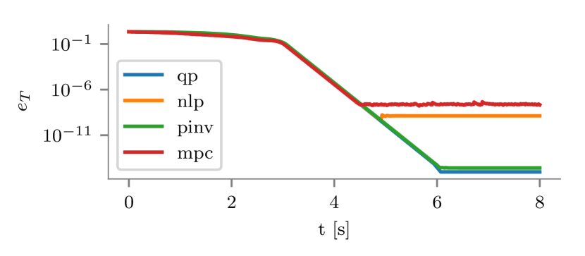
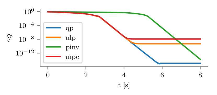
In Fig.3 we see the Euclidean norm of the two representations for each of the controller classes. The null-space approach has a greater error while moving closer to the point as it does not account for the speed saturation. It also struggles more with the dual quaternion formulation and takes a more circuitous route. The different controllers have different limits before numerical issues arise and these may be optimizer settings dependent.

In Tab.II the initial and average runtimes are given for the different controllers during the simulations. The null-space approach is denoted by PINV.

TABLE II: Controller runtimes for Representation Example

	PINV	QP	NLP	MPC
Initial ($\bm{e}_{Q}$)	0.11 ms	0.95 ms	4.23 ms	26.80 ms
Average ($\bm{e}_{Q}$)	0.04 ms	0.27 ms	2.74 ms	20.01 ms
Initial ($\bm{e}_{T}$)	0.09 ms	1.44 ms	4.37 ms	16.90 ms
Average ($\bm{e}_{T}$)	0.04 ms	0.26 ms	2.81 ms	147.08 ms

The NLP approach uses approximately half the control duration, and MPC approach generally uses an order of magnitude longer. This means that the controllers would not be applicable to this control situation with the default settings. The QP approach and null-space approach have applicable timings with the QP approach being an order of magnitude slower than the null-space approach. The average runtime of the MPC formulation with transformation matrix formulation is much higher as a result of using the Frobenius norm and matrix operations. This is likely caused by the prediction constraints becoming more difficult to apply.

IV-B Set Constraints - Bounded Workspace

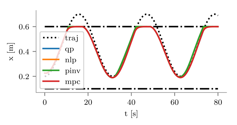
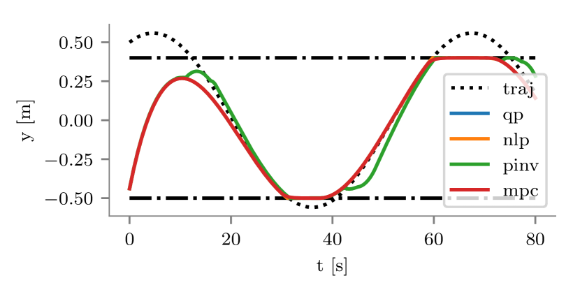
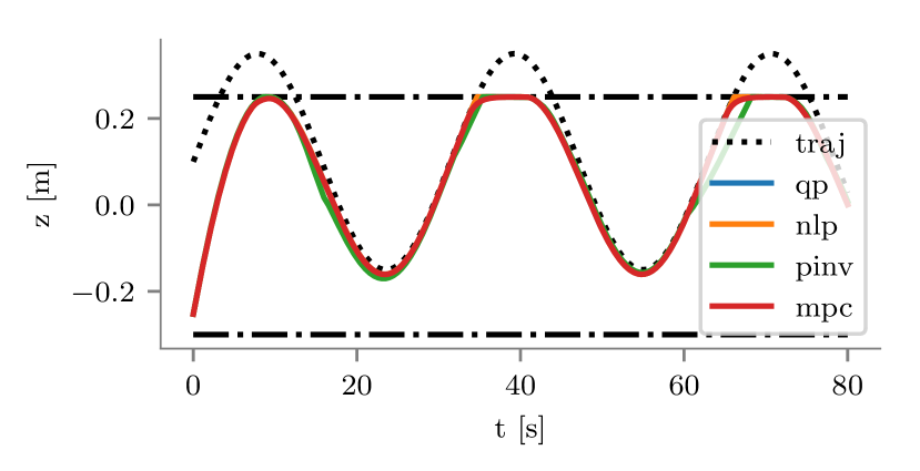
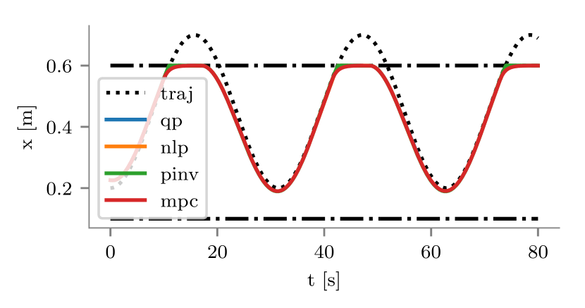
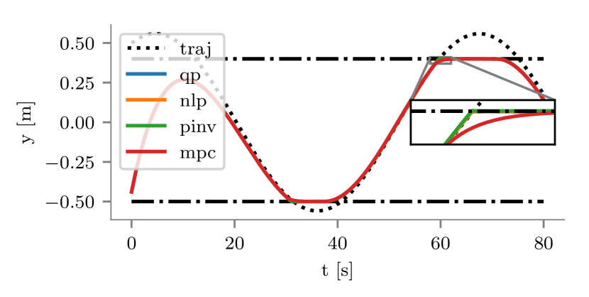
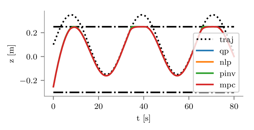
This is a recreation of Example 2 from [6] where a UR5 tracks a Cartesian trajectory while not escaping a box defined workspace. The forward kinematics are defined by the Denavit-Hartenberg parameters in [6] using urdf2casadi.

Figure 4: RViz visualization of the bounded workspace example.

The output function is defined by

$$\bm{e}(t,\bm{q})=\bm{p}(\bm{q})-\bm{p}_{des}(t)$$ (42)

where $\bm{p}(\bm{q})$ is the forward kinematics to the origin of the end-effector, and

$$\bm{p}_{des}(t)=\begin{bmatrix}0.5\sin^{2}(0.1t)+0.2\\ 0.5\cos(0.1t)+0.25\sin(0.1t)\\ 0.5\sin(0.1t)\cos(0.1t)+0.7\end{bmatrix}.$$ (43)

The set constraint is defined by $\bm{p}(\bm{q})\in[\bm{p}_{l},\bm{p}_{u}]$ with $\bm{p}_{l}=[0.1,-0.5,0.3]$ and $\bm{p}_{l}=[0.5,0.4,0.85]$. Examples of the code used to define the equality and set constraints can be seen in Listing.1 and Listing.2, where p(q) and p_d(t) are CasADi functions for end-effector position and desired position, and t and q are MX symbols for time and robot variable. For the null-space projection approach the set constraint can either be formulated using the experimental multidimensional set constraint, or as three separate constraints for $x$, $y$, and $z$ as in [6]. The equality constraint has a lower priority (3rd) such that it can work with either formulation.

Listing 1: Equality Constraint Example

⬇

track_cnstr = EqualityConstraint(

label="tracking_constraint",

expression=p(q) - p_d(t),

gain=1.0,

constraint_type="soft",

priority=3

)

Listing 2: Set Constraint Example

⬇

box_cnstr = SetConstraint(

label="box_constraint",

expression=p(q),

set_min = np.array([0.1, -0.5, 0.3]),

set_max = np.array([0.5, 0.4, 0.85]),

gain = 100.0,

constraint_type="hard",

priority=1

)

From Fig.1 we know that the approach speed to the upper or lower bound on a set constraint are determined by the gain in the optimization approaches. This can be seen as an exponential decay in the tracking task as we approach the set limits. From Fig.2 we see that as the gain approaches $\infty$, we will have the same sharp change when approaching a set limit as the null-space approach exhibits. In this example the set gain is 100 for the QP and NLP. The MPC has gains of 1 as large set gains may lead to more difficult predicted constraints.

In Fig.5 we see the position of the end-effector for the different controllers when handling $x$, $y$, and $z$ as separate constraints and in Fig.6 we see the position when handling them as a single multidimensional constraint.

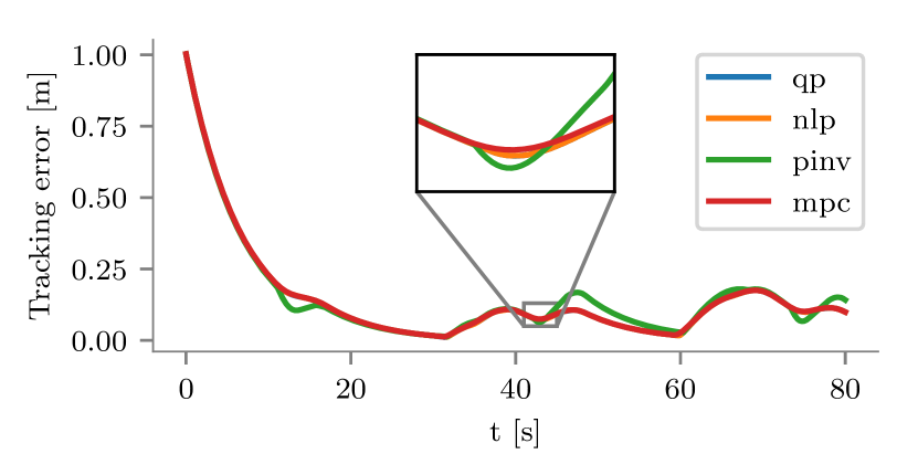
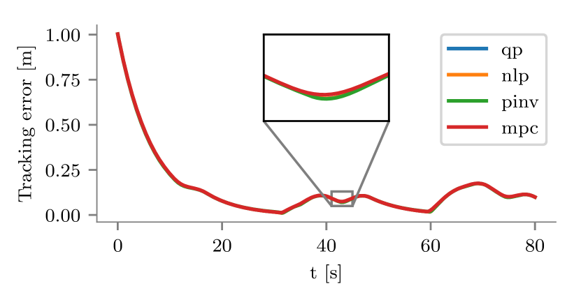
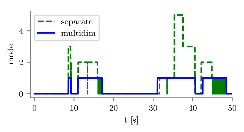
In Fig.7 we see the tracking error with the different controllers when handling $x$, $y$, and $z$ constraints as separate constraints. In Fig.8 we see the tracking error with the different controllers when handling $x$, $y$, and $z$ as a single multidimensional constraint. Similar to the results in [25], setting the constraints in a priority ordered sequence causes unwanted behavior. The multidimensional formulation gives a more correct interpretation of the constraint. Also note that the multidimensional null-space approach and the optimization approaches are similar. If more set constraints are included, such as joint limits, the two methods will differ again. In Fig.9 we see the mode the null-space based controller is in for both the separate $x$, $y$, and $z$ formulation and the multidimensional formulation. The “noisy” rapid switching of modes occurs due to numerical issues with the linearization and the comparison between current and set limits. Tuning either the control duration or the comparison with some numerical lower limit can mitigate this effect.

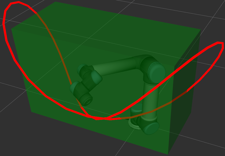
Fig.4 shows a visualization of the controller running with the DefaultRobotInterface and ROS.

(a) $x$

(b) $y$

Figure 5: Position of the end-effector for $x$, $y$, $z$ controlled separately. $z$ omitted for brevity.

(a) $x$

(b) $y$

(c) $z$

Figure 6: Position of the end-effector for $x$ , $y$, $z$ controlled using a multidimensional constraint. The MPC approach exhibits the exponential approach to the constraint limit.

Figure 7: Tracking error for $x$, $y$, and $z$ as separate constraints. The error does not converge to zero as the desired trajectory goes out of the box.

Figure 8: Tracking error for $x$, $y$ and $z$ as a multidimensional constraint. The error does not converge to zero as the desired trajectory goes outside the box. All are equal except MPC which deviates slightly.

Figure 9: Excerpt of the mode the null-space based controller is in for both separate constraints and multidimensional constraints. Note the rapid switching at $t=15$s and $t=45$s when using separate constraints.

IV-C Nonlinear cost - Manipulability Index

In this example a 7 degrees of freedom KUKA LWR IIWA 14 R820 arm is to follow a circular trajectory in its workspace and maximize the manipulability index of the task. The forward kinematics are defined by the URDF and urdf2casadi. The robot is simulated at joint velocity level with Euler discretization. IIWA has $\bm{q}\in\mathbb{R}^{7}$ where $\bm{q}\in[-\bm{q}_{u},\bm{q}_{u}]$ with

$$\bm{q}_{u}^{T}=[170^{\circ},120^{\circ},170^{\circ},120^{\circ},170^{\circ},120^{\circ},175^{\circ}].$$ (44)

The circular trajectory is defined by:

$$\bm{p}_{d}(t)=\begin{bmatrix}0.1\cos(0.05t-0.5\pi)+0.45\\ 0.1\sin(0.05t-0.5\pi)+0.4\\ 0.3\end{bmatrix}.$$ (45)

We define the manipulability index of the task as

$$m(\bm{q})=\sqrt{\det\left(\frac{\partial\bm{p}}{\partial\bm{q}}(\bm{q})\frac{\partial\bm{p}}{\partial\bm{q}}(\bm{q})^{T}\right)}$$ (46)

where $m$ is a measure of the area of the ellipsoid that the Jacobian of the end-effector position forms. We want to both achieve the task and to maximize our manipulability. Maximizing the manipulability can be beneficial in collision avoidance, as a high manipulability means we have more options as to which direction we can move to avoid collision. Maximizing the manipulability can be achieved by adding a term to the nonlinear costs of the NLP and the MPC approach:

$$m_{c}(\bm{q},\dot{\bm{q}})=-\alpha m(\bm{q}+\Delta_{t}\dot{\bm{q}})^{2}$$ (47)

where $\Delta_{t}$ is the control duration and $\alpha$ is set to $500$. This essentially states that we attempt to maximize the manipulability of the subsequent step. Optimization problems often struggle with square roots, so we square the manipulability index before using it in the cost. As the tracking constraint is of lower priority than the joint limits, we must ensure that the tracking constraint’s slack weight is greater than $\alpha$. In Listing 3, we see an example of setting its slack weight to $2000$. The QP approach and null-space approach does not support nonlinear costs and do not maximize their manipulability. The MPC has a horizon length of 10 control steps.

Listing 3: Equality Constraint With Slack Weight

⬇

track_cnstr = EqualityConstraint(

label="tracking_constraint",

expression=p(q) - p_d(t),

gain=1.0,

constraint_type="soft",

slack_weight=2e3

)

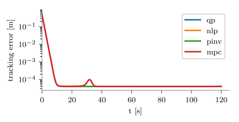
In Fig.10 we see the tracking error over time. The lower limit stems from the linearization assumption, and one must either use a path-following approach, or use lower control durations to overcome this. At $t=30$s, the MPC approach is able to find a different configuration with higher manipulability at the cost of a short duration of deviating from the trajectory. This reconfiguration does not affect the final tracking error of the MPC.

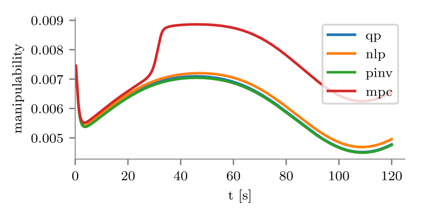
In Fig.11 we see the manipulability index $m$ over time. The NLP performs slightly better than the QP approach, and the MPC performs best by far as it chooses to deviate slightly from the trajectory to arrive at a configuration with a higher manipulability.

Figure 10: Tracking error when following the circular trajectory. The MPC approach deviates slightly at $t=30$s as it is reconfiguring to an orientation with higher manipulability.

Figure 11: Manipulability index for different controllers over time when tracking the circular trajectory. The MPC approach is able to find a configuration with higher manipulability index at $t=30s$.

TABLE III: Controller runtimes for Manipulability Example

	PINV	QP	NLP	MPC
Initial	0.11 ms	0.48 ms	4.94 ms	54.72 ms
Average	0.07 ms	0.19 ms	3.02 ms	49.52 ms

In Tab.III we see the initial and average runtimes of the different controllers. The inclusion of the manipulability cost has not made the controllers deviate from the rule of an order of magnitude separation between the approaches.

IV-D Input - Tracking a marker in ROS

Figure 12: RViz visualization of tracking an input marker.

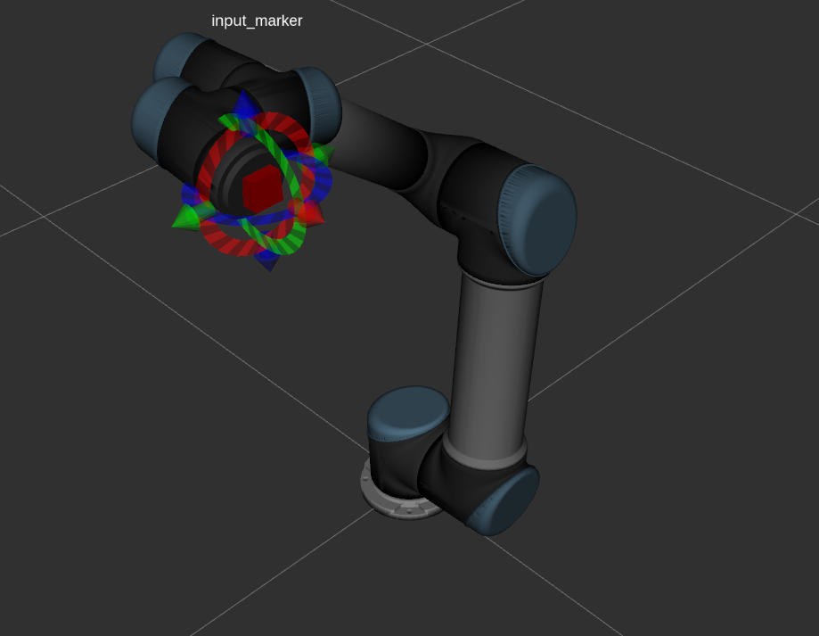
In this example a UR5 robot tries to track user input. The DefaultRobotInterface is used with ROS and an RViz interactive marker to simulate an external input. The robot is simulated with Gazebo and is controlled at 50 Hz. We use the QP approach in this example. The maximum joint speed is $3$ rad/s.

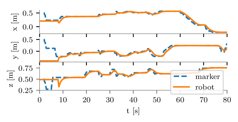
In Fig.13 we see the position of the marker and the end-effector frame. The end-effector has an exponential convergence to the desired input marker position, but as it does not consider the speed of the input marker, there is a tracking error when following the input marker during a continuous motion. The DefaultRobotInterface has a delay of 7.8s before it starts as it waits for topics and compiles the controller.

Figure 13: Position of the input marker and end-effector frame when tracking the input marker.

IV-E Velocity Equality Constraint - 6 DOF compliance

Figure 14: Experimental setup for 6 DOF compliance.

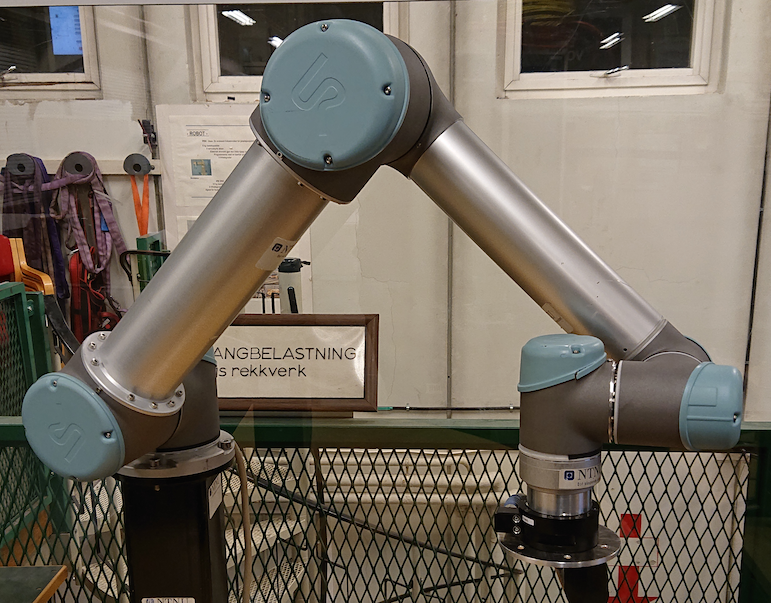
In this example the end-effector of a UR5 is to comply to forces and torques acting on it. The example uses urdf2casadi to determine forward kinematics, and ur_modern_driver[30]. The end-effector has an ATI Mini45 force/torque sensor attached with a mounting plate on it. The robot is in an open workspace. To ensure the robot does not crash with the table or is moved to undesired regions, the end-effector is limited to a box. The box is defined by the set constraint

$$\begin{bmatrix}-0.7\\ -0.4\\ -0.2\end{bmatrix}\leq\bm{p}(\bm{q})\leq\begin{bmatrix}-0.3\\ 0.5\\ 0.5\end{bmatrix}.$$ (48)

Velocity resolved compliance can be achieved using damping control[33] by

$$\begin{bmatrix}\bm{v}(t)\\ \bm{\omega}(t)\end{bmatrix}=\begin{bmatrix}K_{f}\bm{f}(t)\\ K_{\tau}\bm{\tau}(t)\end{bmatrix}$$ (49)

where $\bm{v}$ is the Cartesian velocity, $\bm{\omega}$ is the rotational velocity, $\bm{f}$ are the linear forces, and $\bm{\tau}$ are the torques. All evaluated at the end-effector. $K_{f}$ and $K_{\tau}$ are the damping constants for the forces and torques respectively.

For linear forces $\bm{f}$ acting on the end-effector, and a position $\bm{p}(t)$ of the end-effector, we desire:

$$\dot{\bm{p}}(t)=K_{f}\bm{f}^{w}(t)=K_{f}\bm{R}(\bm{q})\bm{f}(t)$$ (50)

where $\bm{f}^{w}$ are the forces acting on the end-effector represented in the world coordinates.

We can relate the rotational velocity to the derivative of the orientation quaternion by following [34], and arrive at

$$\dot{\bm{Q}}_{r}(t)=\frac{K_{\tau}}{2}\bar{\bm{H}}\left(\begin{bmatrix}\bm{\tau}(t)\\ 0\end{bmatrix}\right)\bm{Q}_{r}(t)$$ (51)

where $\bm{\tau}(t)$ are the torques acting on the end-effector in the end-effector frame.

An example of the constraint is given in Listing 4.

Listing 4: Velocity Equality Constraint Example

⬇

comply_cnstr = VelocityEqualityConstraint(

label="comply_constraint",

expression=vertcat(p(q), Q_rot(q)),

target=vertcat(Kf*p(q),

0.5*Kt*mtimes(H(tau,0), Q_rot(q))),

constraint_type="soft"

)

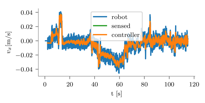
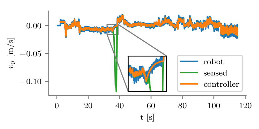
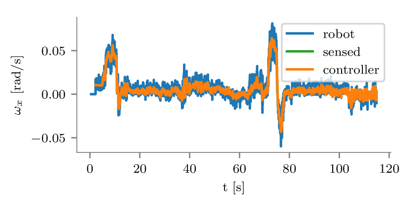
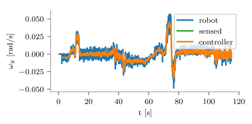
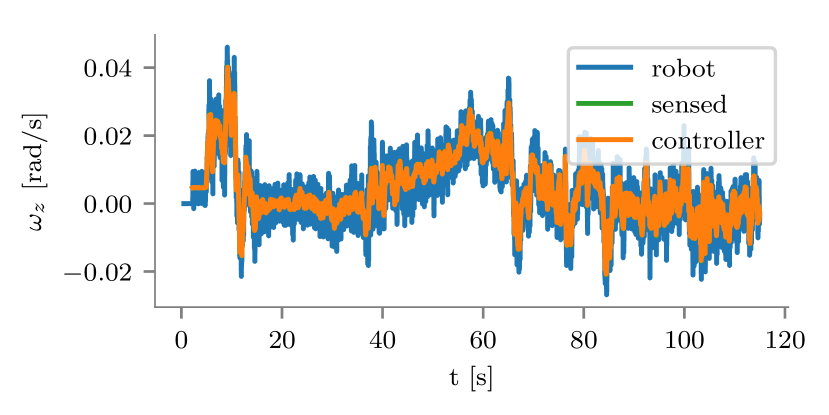
The controller is running at 125 Hz, and the force/torque sensor runs at 250 Hz but only the most recent value is used. The damping factors are $K_{f}=0.01$ and $K_{t}=0.1$. This experiment was run with the QP controller. To inspect the behavior of the system we look at the right hand side of (50) and (51) with the sensor value for force, torque, and $\bm{q}$. We refer to this as sensed speed. The left hand side of (50) and (51) as desired by the CASCLIK controller or as reported by the robot, is referred to as the controller speed and the robot speed respectively.

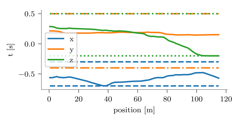
In Fig.15 we see the position of the end-effector over time. In Fig.16 we see sensed speed, controller speed and robot speed. The controller moves to track the target function, resulting in compliance of the end-effector with respect to the force. In Fig.17 we comply with respect to the torques. From $t=36$s until $t=40$ we try to pull the end-effector out of the box constraint. As the robot approaches the box constraint, the compliance is reduced to zero. At $t=80$s we let go of the end-effector and sensor bias moved it slowly to the bottom and along the bottom of the box constraint. The noise is both a result of the latency introduced by using ROS for real-time feedback control, by the computation time of the controller, and by inherent noise in the joint speed signal.

Figure 15: Position over time of the end-effector during the velocity equality experiment for compliance. The stippled and dotted lines denote the box constraint. From $t=36$s until $t=40$s we attempt to pull the end-effector out of the box constraint in $x$ direction, but the set constraint does not allow it. At $t=80$s we let go of the end-effector, and it drifted to the bottom of the box due to sensor bias.

(a) Complying with $f_{x}$

(b) Complying with $f_{y}$

(c) Complying with $f_{z}$

Figure 16: Sensor and controller Cartesian speeds (right and left hand side of (50)), and robot Cartesian speeds of the end-effector. The zoomed inset at $t=36$s in subfigure (b) shows the exponential convergence to zero speed in $z$ direction as we try to pull the end-effector out of the box constraint. Otherwise, the sensed and controller speeds perfectly overlap as long as we are inside the box.

(a) Complying with $\tau_{x}$

(b) Complying with $\tau_{y}$

(c) Complying with $\tau_{z}$

Figure 17: Sensor and controller angular speed (right and left hand side of (51)), and robot angular speeds of the end-effector. As the box constraint only considers the position of the end-effector, not the orientation, the box constraint does not affect the torque compliance.

V Discussion

Closed-loop inverse kinematics frameworks handle local problems rather than global problems. When given desired positions far from the current position, closed-loop inverse kinematics may succumb to local minima. This means that they are mid-level controllers to which a desired path may be supplied from a high-level path planner. The model predictive controller formulation is an attempt at bridging the gap between local and global planning. Proper design of cost and constraint formulations to better achieve tasks may lead to better handling of local minima. As of yet, the model predictive approach is significantly slower than its reactive counterparts and further work includes investigating sequential quadratic programming approaches with warmstart as they may have shorter execution time than the non-warmstarted interior point method of IPOPT. By using CasADi at the core, CASCLIK can quickly benefit from any new solver implemented in CasADi. The lack of convexity of the constraints along the prediction horizon in the current formulation also suggests that further work should be done to investigate the optimality and stability of the approach.

CASCLIK is independent of the underlying representation used to define kinematics. This allows for inspecting behavior of different representations, but complicates programming for the user. A more robust framework can be created by defining the underlying representation. The choice of using arbitrary functions is a design choice intended to allow a larger range of scenarios and systems to be handled by CASCLIK as well as being easier to implement. Future work includes examining other coordinate representations and constraints.

From the input experiments we see that the controllers have an exponential convergence to the reference signal during positioning, and classical compliance can be implemented in CASCLIK for the controllers that accept velocity equality constraints. As sensors are becoming cheaper and more available, it is important to allow for arbitrary input signals. As the derivative of inputs are unknown, they are considered to be zero. For input signals such as distance sensors or force sensors, this is a false assumption and can lead to tracking error for time varying sensor signals. Future work includes allowing the user to provide input derivatives for CASCLIK. These may come from speed observers, derivative filters, or any other sources the user provides.

CASCLIK only considers control at the velocity setpoint level. This stems from the main use-case for which the framework was intended, industrial manipulators. In most cases, industrial manipulators only provide joint position or joint velocity setpoints. However, the task function approach allows for specifying control at the acceleration or torque level [2]. Extending CASCLIK to include acceleration resolved controllers would allow specifying velocity constraints that ensure convergence to the desired velocity.

Although CasADi is intended for prototyping, C code generation is possible. This could allow for specifying tasks and controllers with CASCLIK before deploying the controller to an embedded system. For control from an external computer the just-in-time compilation feature of CasADi allows for defining quadratic problem or null-space based controllers that can be run at $\leq$1 ms speeds, which can allow for employing CASCLIK on real systems. However, for industrial use-cases and real-time sensitive systems, the authors recommend eTaSL/eTC [7]. Many robot systems have limits on acceleration or jerk applied to the system, further work includes investigating methods of implementing such constraints in CASCLIK.

From the examples, we see that the null-space approach has similar behavior to the optimization approaches when handling a single set constraint with very high gain. For multiple tasks, the null-space projection operator will cause the set-based task priority framework to behave differently from the optimization approaches. The optimization approaches uses slack variables to handle multiple tasks. This moves prioritization into the cost expression of the optimization problem and does not allow for strict prioritization between tasks, but tuning of the slack weight can be used to specify different behavior of the tasks. As strict prioritization may be desired in certain cases, future work includes creating a hybrid approach that uses the optimization approach to define the desired control variables for certain tasks, and the null-space projection to ensure strict priority of other tasks.

The optimization approaches are closely related, and the complexity of implementing them is similar. The null-space approach requires more bookkeeping by the programmer but generally provides controllers with shorter execution time. Generally the execution speeds are in the order: null-space approach, QP approach, NLP approach, and MPC approach. Each increasing by an order of magnitude in the sequence, depending on the horizon length of the MPC. For rapid prototyping and large set of tasks, the compilation time may also be of interest. As the null-space approach compiles each separate mode, and there are $2^{n_{set}}$ modes, its compilation time drastically increases with multiple set constraints.

The nonlinear cost example shows that the NLP and MPC approach can improve the manipulability in cases where the QP and null-space approach did not. Although the MPC approach managed to find an alternative configuration that increased the manipulability significantly, the reactive NLP approach did not. As the manipulability cost can be added to the QP formulation via Taylor expansion of the cost as in [35], the NLP approach may not be as beneficial as initially expected.

VI Conclusion

In this paper, CASCLIK, a rapid prototyping framework for multiple task-based closed-loop inverse kinematics controllers is presented. It translates tasks into quadratic, nonlinear, or model predictive optimization problems that can be solved with CasADi. Tasks are formulated as constraints, and multiple tasks can be achieved simultaneously.

CASCLIK also provides a CasADi based implementation of the set-based task priority inverse kinematics framework. The paper includes a novel multidimensional formulation of the in tangent cone function such that the set-based task priority framework can support multidimensional set constraints. The results show that the multidimensional set constraint formulation can give a better representation of the desired behavior than when a multidimensional set constraint is split into multiple one dimensional constraints.

References

- [1] L. Sciavicco and B. Siciliano, “Coordinate Transformation: A Solution Algorithm for One Class of Robots,” IEEE Transactions on Systems, Man and Cybernetics, vol. 16, no. 4, pp. 550–559, 1986.
- [2] C. Samson, M. Le Borgne, and B. Espiau, Robot Control: The Task Function Approach, 1st ed. New York: Oxford University Press, 1991.
- [3] J. De Schutter, T. De Laet, J. Rutgeerts, W. Decré, R. Smits, E. Aertbeliën, K. Claes, and H. Bruyninckx, “Constraint-based Task Specification and Estimation for Sensor-Based Robot Systems in the Presence of Geometric Uncertainty,” The International Journal of Robotics Research, vol. 26, no. 5, pp. 433–455, may 2007.
- [4] H. Hanafusa, T. Yoshikawa, and Y. Nakamura, “Analysis and Control of Articulated Robot Arms with Redundancy,” IFAC Proceedings Volumes, vol. 14, no. 2, pp. 1927–1932, 1981.
- [5] S. Chiaverini, “Singularity-robust task-priority redundancy resolution for real-time kinematic control of robot manipulators,” IEEE Transactions on Robotics and Automation, vol. 13, no. 3, pp. 398–410, 1997.
- [6] S. Moe, G. Antonelli, A. R. Teel, K. Y. Pettersen, and J. Schrimpf, “Set-Based Tasks within the Singularity-Robust Multiple Task-Priority Inverse Kinematics Framework: General Formulation, Stability Analysis, and Experimental Results,” Frontiers in Robotics and AI, vol. 3, no. April, pp. 1–18, 2016.
- [7] E. Aertbelien and J. De Schutter, “eTaSL/eTC: A constraint-based task specification language and robot controller using expression graphs,” in IEEE International Conference on Intelligent Robots and Systems. IEEE, sep 2014, pp. 1540–1546.
- [8] J. Andersson, “A General-Purpose Software Framework for Dynamic Optimization,” PhD thesis, Arenberg Doctoral School, KU Leuven, Belgium, 2013.
- [9] H. J. Ferreau, C. Kirches, A. Potschka, H. G. Bock, and M. Diehl, “qpOASES: a parametric active-set algorithm for quadratic programming,” Mathematical Programming Computation, vol. 6, no. 4, pp. 327–363, 2014.
- [10] A. Wächter and L. T. Biegler, “On the implementation of an interior-point filter line-search algorithm for large-scale nonlinear programming,” Mathematical Programming, vol. 106, no. 1, pp. 25–57, mar 2006.
- [11] M. H. Arbo, Y. Pane, E. Aertbeliën, and W. Decre, “A System Architecture for Constraint-Based Programming of Robotics Assembly with CAD Information,” in IEEE International Conference on Automation Science and Engineering, 2018.
- [12] N. Mansard, O. Khatib, and A. Kheddar, “A Unified Approach to Integrate Unilateral Constraints in the Stack of Tasks,” IEEE Transactions on Robotics, vol. 25, no. 3, pp. 670–685, jun 2009.
- [13] “Stack-of-tasks.” [Online]. Available: http://stack-of-tasks.github.io/
- [14] A. Escande, N. Mansard, and P. B. Wieber, “Hierarchical quadratic programming: Fast online humanoid-robot motion generation,” International Journal of Robotics Research, vol. 33, no. 7, pp. 1006–1028, 2014.
- [15] R. Smits, T. De Laet, K. Claes, H. Bruyninckx, and J. De Schutter, “iTASC: a tool for multi-sensor integration in robot manipulation,” in 2008 IEEE International Conference on Multisensor Fusion and Integration for Intelligent Systems. IEEE, aug 2008, pp. 426–433.
- [16] “OROCOS: iTaSC wiki.” [Online]. Available: http://orocos.org/wiki/orocos/itasc-wiki/2-itasc-software
- [17] H. Bruyninckx, P. Soetens, and B. Koninckx, “The real-time motion control core of the Orocos project,” 2003 IEEE International Conference on Robotics and Automation (Cat. No.03CH37422), pp. 2766–2771, 2003.
- [18] P. Soetens, “RTT: Real-Time Toolkit.” [Online]. Available: http://www.orocos.org/rtt
- [19] E. Aertbeliën, “expressiongraphs.” [Online]. Available: https://github.com/eaertbel/expressiongraph
- [20] R. Smits, “KDL: Kinematics and Dynamics Library.” [Online]. Available: http://www.orocos.org/kdl
- [21] N. Somani, M. Rickert, A. Gaschler, C. Cai, A. Perzylo, and A. Knoll, “Task level robot programming using prioritized non-linear inequality constraints,” IEEE International Conference on Intelligent Robots and Systems, vol. 2016-Novem, pp. 430–437, 2016.
- [22] N. Somani, M. Rickert, and A. Knoll, “An Exact Solver for Geometric Constraints With Inequalities,” IEEE Robotics and Automation Letters, vol. 2, no. 2, pp. 1148–1155, apr 2017.
- [23] A. Perzylo, N. Somani, S. Profanter, I. Kessler, M. Rickert, and A. Knoll, “Intuitive instruction of industrial robots: Semantic process descriptions for small lot production,” in 2016 IEEE/RSJ International Conference on Intelligent Robots and Systems (IROS), vol. 2016-Novem. IEEE, oct 2016, pp. 2293–2300.
- [24] G. Antonelli, G. Indiveri, and S. Chiaverini, “Prioritized closed-loop inverse kinematic algorithms for redundant robotic systems with velocity saturations,” 2009 IEEE/RSJ International Conference on Intelligent Robots and Systems, IROS 2009, no. 3, pp. 5892–5897, 2009.
- [25] M. H. Arbo and J. T. Gravdahl, “Stability of the Tracking Problem with Task-Priority Inverse Kinematics,” in 12th IFAC Symposium on Robot Control SYROCO 2018, vol. 51, no. 22, Budapest, 2018, pp. 121–125.
- [26] S. Boyd and L. Vandenberghe, Convex Optimization. Cambridge: Cambridge University Press, 2004.
- [27] “A000788: Total number of 1’s in binary expansions of 0, …, n.” [Online]. Available: https://oeis.org/A000788
- [28] A. Colome and C. Torras, “Closed-loop inverse kinematics for redundant robots: Comparative assessment and two enhancements,” IEEE/ASME Transactions on Mechatronics, vol. 20, no. 2, pp. 944–955, 2015.
- [29] M. H. Arbo, “Mathias Hauan Arbo’s Github page.” [Online]. Available: https://github.com/mahaarbo/
- [30] T. T. Andersen, “Optimizing the Universal Robots ROS driver.” Technical University of Denmark, Department of Electrical Engineering, Tech. Rep., 2015.
- [31] L. F. Figueredo, B. V. Adorno, J. Y. Ishihara, and G. A. Borges, “Robust kinematic control of manipulator robots using dual quaternion representation,” Proceedings - IEEE International Conference on Robotics and Automation, pp. 1949–1955, 2013.
- [32] P. M. Larochelle, A. P. Murray, and J. Angeles, “A Distance Metric for Finite Sets of Rigid-Body Displacements via the Polar Decomposition,” Journal of Mechanical Design, vol. 129, no. 8, p. 883, 2007.
- [33] B. Siciliano and O. Khatib, Springer Handbook of Robotics. Springer Science & Business Media, 2008.
- [34] X. Wang, D. Han, C. Yu, and Z. Zheng, “The geometric structure of unit dual quaternion with application in kinematic control,” Journal of Mathematical Analysis and Applications, vol. 389, no. 2, pp. 1352–1364, 2012.
- [35] K. Dufour and W. Suleiman, “On integrating manipulability index into inverse kinematics solver,” in IEEE International Conference on Intelligent Robots and Systems, vol. 2017-Septe, 2017, pp. 6967–6972.