HARPS-N radial velocities confirm the low densities of the Kepler-9 planets

Abstract

We investigated the discrepancy between planetary mass determination using the transit timing variations (TTVs) and radial velocities (RVs), by analysing the multi-planet system Kepler-9. Despite being the first system characterised with TTVs, there are several discrepant solutions in the literature, with those reporting lower planetary densities being apparently in disagreement with high-precision RV observations. To resolve this, we gathered HARPS-N RVs at epochs that maximised the difference between the predicted RV curves from discrepant solutions in the literature. We also re-analysed the full Kepler data-set and performed a dynamical fit, within a Bayesian framework, using the newly derived central and duration times of the transits. We compared these results with the RV data and found that our solution better describes the RV observations, despite the masses of the planets being nearly half that presented in the discovery paper. We therefore confirm that the TTV method can provide mass determinations that agree with those determined using high-precision RVs. The low densities of the planets place them in the scarcely populated region of the super-Neptunes / inflated sub-Saturns in the mass-radius diagram.

1 Introduction

One of the most important accomplishments of the Kepler mission (Borucki et al., 2011) is the demonstration that transit timing variation (TTV) is a powerful tool to estimate the masses of planets around stars (Agol et al., 2005; Holman & Murray, 2005) that are too faint for a proper radial velocity (RV) follow-up. Notable early examples are the characterisation of the two Saturn-like planets around Kepler-9 (Holman et al., 2010), a system of five low-mass, small-size planets around Kepler-11 (Lissauer et al., 2011), and the three-planet system around Kepler-18 (Cochran et al., 2011). However, with the increasing number of well-characterised, low-mass planets, a marked difference in the density distribution of planets with TTV- and RV-derived masses has started to appear. This suggests the presence of an intrinsic problem with one of the two techniques (Weiss & Marcy, 2014). Subsequent studies on individual systems involving both TTV and RVs, such as WASP-47 (Becker et al., 2015; Weiss et al., 2016), K2-19 (Barros et al., 2015; Nespral et al., 2017) and Kepler-19 (Malavolta et al., 2017a), as well as ensemble studies on system with different characteristics (Jontof-Hutter et al., 2016) and statistical analysis on simulated observations (Steffen, 2016; Mills & Mazeh, 2017), showed that both techniques lead to similar results, and the discrepancy in planetary density is likely the result of an observational bias. In some cases inconsistencies between TTV and RV masses still persist, as for KOI-94d where the dynamical mass (Masuda et al., 2013) is half the mass obtained by high-precision RVs (Weiss et al., 2013). For this reason it is important to analyse as many systems as possible with both techniques.

In this paper we focus on the planetary system around Kepler-9, a faint (V=13.9) Sun-like star. From the analysis of the three quarters of Kepler data, Holman et al. (2010, hereafter H10) identified two transiting Saturn-size planets with periods and radii of $P_{\mathrm{b}}=19.24$ d, $R_{\mathrm{b}}=9.4\,R_{\oplus}$ and $P_{\mathrm{c}}=38.91$ d, $R_{\mathrm{c}}=9.2\,R_{\oplus}$ respectively, and another transiting body validated by Torres et al. (2011) as a super-Earth size planet with period and radius of $P_{\mathrm{d}}=1.59$ d, $R_{\mathrm{d}}=1.64\,R_{\oplus}$. Using TTVs coupled with 6 RV measurements obtained with Keck-HIRES they determined a mass of $80.0\pm 4.1M_{\oplus}$ for Kepler-9b and $54.3\pm 4.1\,M_{\oplus}$ for Kepler-9c. A subsequent work by Borsato et al. (2014, hereafter B14) nearly halved the mass determinations, $M_{\mathrm{b}}=43.5\pm 0.6\,M_{\oplus}$ and $M_{\mathrm{c}}=29.8\pm 0.6\,M_{\oplus}$. The new analysis was performed using time of transits ($T_{0}$s) extracted from 12 Kepler quarters, but the HIRES RVs were excluded because the combined fit was not particularly good. Both results were obtained using a two-planet model, since the TTV amplitude induced by Kepler-9d (Torres et al., 2011) is expected to be only tens of seconds, and is, hence, too low to be measured in the Kepler long-cadence data (Holman et al., 2010). Very recently, these results were confirmed by Freudenthal et al. (2018) within the project Kepler Object of Interest Network (KOINet, von Essen et al., 2018). Using a photodynamical model they analysed the photometric data of all the 17 Kepler quarters and 13 new ground-based light curves. The Keck-HIRES data are not consistent with their solution, as in B14, and the discrepancy has been ascribed to stellar activity.

The two Saturn-like planets in the Kepler-9 system belong to the small group of planets whose masses can be obtained dynamically by modelling the TTVs and whose RV signals are detectable with current facilities. However, the two sets of solutions actually available in the literature for this system are either partially inconsistent with transit timings obtained after the publication of the discovery paper (H10) or with high-precision RVs (B14 and following analyses), and this inconsistency has never been dealt with in any work. For this reason we decided to observe the target with HARPS-N, the high-precision velocimeter mounted at the Telescopio Nazionale Galileo (La Palma) to understand which of the two solutions is more consistent with an independent set of radial velocities. At the same time we aim to improve the literature values by re-analysing all the 17 Kepler quarters and provide a more robust estimate on the error bars of the orbital parameters. In this work we describe the observational strategy we pursued with HARPS-N within the Guaranteed Time Observations (GTO) program of the HARPS-N Collaboration, the comparison of RVs with the literature solutions, and the details on the determination of the updated orbital parameters.

2 Observational strategy

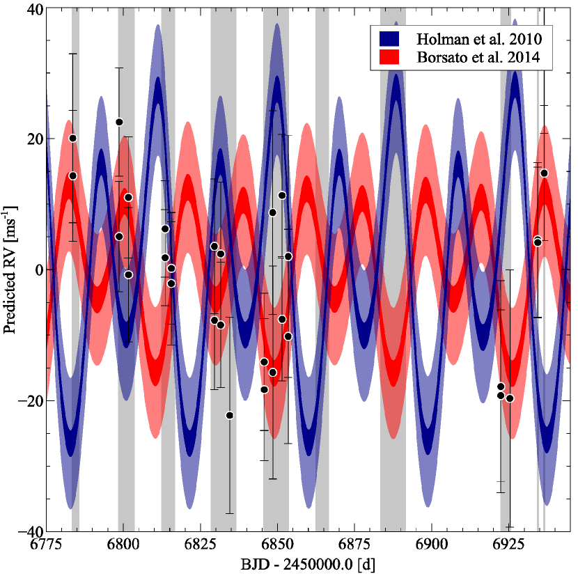
With a magnitude of V=13.9, mass determination of Kepler-9b and c is a very challenging task even for HARPS-N. The planets have an expected RV semi-amplitude of $K_{\mathrm{b}}\simeq 19$ m s^-1 and $K_{\mathrm{c}}\simeq 10$ m s^-1 from the H10 solution, and $K_{\mathrm{b}}\simeq 10$ m s^-1, $K_{\mathrm{c}}\simeq 6$ m s^-1 from the B14 solution. This is comparable with the expected RV error of $\simeq 11$ m s^-1 for a 30-minutes exposure. An independent RV determination of the mass of the planets at 5 $\sigma$ would be extremely time consuming, especially in the case of the low-mass scenario, and it would compete against other Kepler targets more fitting to the science goal of the HARPS-N Collaboration (e. g., precise mass determination of super-Earth and mini-Neptune planets), in the limited window visibility of the Kepler field during a night. For this target we specifically designed an observational strategy that could allow us to distinguish between the two proposed solutions. We first propagated the solution of H10 and B14 to cover the observing season, using the dynamical integrator embedded in TRADES (Borsato et al., 2014). For consistency, we used the same stellar mass of the two papers. Within the nights allocated to HARPS-N Collaboration, we selected those epochs in which the difference between the H10 and B14 expected RVs was at its maximum (Fig. 1). To reduce the CCF noise associated with a single epoch without introducing systematic errors due to the variation of the barycentric radial velocity correction within the exposure time, we gathered - whenever possible - two consecutive 30 minutes exposures. Following this strategy we obtained a total of 16 epochs divided in 30 exposures of 1800s (in two nights only one exposure was taken), with an average signal-to-noise ratio of 16 at 5500 Å and an average internal error of $11.6$ m s^-1 per exposure. Radial velocities were corrected for Moon contamination following the recipe described in Malavolta et al. (2017a) and successfully applied by Osborn et al. (2017). Table 5 lists the final RV measurements.

Figure 1: Scheduling plot: predicted RV model for H10 (blue) and B14 (red), with 2.5 m s^-1 and 10 m s^-1 uncertainties (light and dark shaded areas respectively), used to schedule the HARPS-N observations (white-black circles).

3 Stellar parameters

We followed the same approach described in Malavolta et al. (2018) to determine the mass, radius and density of the star. We started by measuring the photospheric parameters of the target with three different techniques on a spectrum obtained by stacking all the HARPS-N exposures (signal-to-noise ratio $\simeq 90$). Using CCFpams (Malavolta et al., 2017b) we obtained $T_{\mathrm{\rm eff}}=5836\pm 51$ K, $\log g=4.50\pm 0.10$, $[{\rm Fe}/{\rm H}]=0.04\pm 0.04$. The ARES+MOOG, approach (e. g., Mortier et al. 2014) returned $T_{\mathrm{\rm eff}}=5827\pm 35$, $\log g=4.46\pm 0.04$, $[{\rm Fe}/{\rm H}]=0.12\pm 0.03$. Finally with the Stellar Parameters Classification tool (SPC, Buchhave et al. 2012, 2014) we obtained $T_{\mathrm{eff}}=5750\pm 50$ K, $\log g=4.45\pm 0.10$, $[{\rm Fe}/{\rm H}]=-0.02\pm 0.08$. All the reported errors are internal only.

For each set of stellar parameters we then determined the stellar mass and radius using isochrones (Morton, 2015), with posterior sampling performed by MultiNest (Feroz & Hobson, 2008; Feroz, Hobson & Bridges, 2009; Feroz et al., 2013). We provided as input the parallax of the target from the Gaia DR2 catalogue ($p=1.563\pm 0.017$ mas, $d=640\pm 7$ pc, Gaia Collaboration et al. 2016, 2018) with the correction suggested by Stassun & Torres (2018) of $-82\pm 33\ \mu$as, plus the photometry from the Two Micron All Sky Survey (2MASS, Cutri et al. 2003; Skrutskie et al. 2006). For stellar models we used both MESA Isochrones & Stellar Tracks (MIST, Dotter 2016; Choi et al. 2016; Paxton et al. 2011) and the Dartmouth Stellar Evolution Database (Dotter et al., 2008). We performed the analysis on the photospheric parameters obtained with HARPS-N as well as the literature values obtained by H10, Huber et al. (2014), Petigura et al. (2017) and Wang et al. (2018). For all methods we assumed $\sigma_{T_{\mathrm{eff}}}=75$ K, $\sigma_{\log g}=0.10$, $\sigma_{[{\rm Fe}/{\rm H}]}=0.05$ as a good estimate of the systematic errors, when the provided errors were lower than these values.

From the median and standard deviation of all the posterior samplings we obtained $M_{\star}$ $=1.022_{-0.029}^{+0.039}$ M_⊙ and $\mbox{$R_{\star}$}=0.96\pm 0.02\ \mbox{R${}_{\odot}$}$. We derived the stellar density $\rho_{\star}$ $=1.16_{-0.09}^{+0.08}$ $\rho_{\odot}$ directly from the posterior distributions of $M_{\star}$ and $R_{\star}$. Following Lovis et al. (2011), from the individual HARPS-N exposures we measured a $\log{\rm R}^{\prime}_{\rm HK}$ index of $-4.67\pm 0.09$, consistent with the young age of the star ($2.0^{+2.0}_{-1.3}$ Gy) derived from the fit of the isochrones (e. g., Pace 2013). The astrophysical parameters of the star are summarised in Table 1, where the temperature, gravity and metallicity are those obtained from the posterior distributions to take into account the constraint from Gaia parallax. The stellar density determined in this work agrees very well with the value derived in Freudenthal et al. (2018) with the dynamical analysis of the light curve.

Table 1: Astrophysical parameters of the star.

Parameter	Value	Unit
2MASS alias	J19021775+3824032
$\alpha_{\rm J2000}$	19:02:17.76	hms
$\delta_{\rm J2000}$	+38:24:03.2	dms
$R_{\star}$	$0.958\pm 0.020$	R⊙
$M_{\star}$	$1.022_{-0.039}^{+0.029}$	M⊙
$\rho_{\star}$	$1.16_{-0.09}^{+0.08}$	$\rho_{\odot}$
$\log(L_{\star}/L_{\odot})$	$-0.038_{-0.027}^{0.026}$	-
$T_{{\rm eff}}$	$5774\pm 60$	K
$\log g$	$4.49_{-0.03}^{0.02}$	-
$[{\rm Fe}/{\rm H}]$	$0.05\pm 0.07$	-
$p^{(a)}$	$1.643\pm 0.037$	mas
distance	$614\pm 13$	pc
AV	$0.10_{-0.07}^{+0.10}$	mag
B-V	$0.70\pm 0.13$	mag
age	$2.0_{-1.3}^{+2.0}$	Gy
$\log{\rm R}^{\prime}_{\rm HK}$	$-4.67\pm 0.09$	-

^(a) Gaia parallax corrected for systematic offset as suggested by Stassun & Torres (2018).

4 Analysis of the Kepler data

We downloaded the Kepler-9 data from the MAST covering the full 17 quarters of the mission in long (LC) and short (SC) cadence. We used the Presearch Data Conditioning (PDC) fluxes instead of Simple Aperture Photometry (SAP), because the handling of systematic trends and errors were out of the purpose of this work. We created a normalised full light curve by dividing the PDC flux of each quarter by its median value. We selected carefully the portion of the transits and the out-of-transit, in particular when the light curve shows transit events of Kepler-9b and Kepler-9c very close to each other.

For each light curve we fitted the following parameters: $\log_{10}\rho_{\star}$ where $\rho_{\star}$ is the stellar density in kg m^-3, $\sqrt{k}$ where $k$ is the ratio between the planetary and the stellar radii, $\sqrt{b}$ where $b$ is the impact parameter, the central time of the transit ($T_{0}$), a quadratic limb-darkening (LD) law with the parameters $q_{1}$ and $q_{2}$ introduced in Kipping (2013), a linear trend (with $a_{0}$ as the intercept and $a_{1}$ the angular coefficient), and $\log_{2}\sigma_{j}$, where $\sigma_{j}$ is a jitter term to add in quadrature to the errors of the Kepler light curve. We used an asymmetric prior for the $\log_{10}\rho_{\star}$ based on the stellar mass and radius values determined in section 3, while we used a uniform prior for the other parameters (see Table 2); we kept fixed the period ($P$), the eccentricity and argument of pericentre (values from B14 solution).

We ran a Differential Evolution algorithm (Storn & Price, 1997, pyDE) and then a Bayesian analysis of each selected light curve around each transit by using the affine-invariant ensemble sampler (Goodman & Weare, 2010) for Markov chain Monte Carlo (MCMC) implemented within the emcee package (Foreman-Mackey et al., 2013) and modelling each transit with batman (Kreidberg, 2015). We took into account the long exposure time of the LC data oversampling the transit model; for consistency, we used the same oversampling also for the SC data.

Table 2: Table of the priors, boundaries, and final solution of the fitted parameters for transit analysis and the derived parameters.

parameter	prior type	boundaries [min, max]	Kepler-9b	Kepler-9c
$\log_{10}\rho_{\star}$	G	$[0.,6.]$	$3.196_{-0.060}^{+0.046}$	$3.188_{-0.067}^{+0.048}$
$\sqrt{k}$	U	$[0.,1.]$	$0.2786_{-0.0030}^{+0.0033}$	$0.2750_{-0.0027}^{+0.0033}$
$\sqrt{b}$	U	$\left[0.,\sqrt{2}\right]$	$0.767_{-0.035}^{+0.042}$	$0.861_{-0.022}^{+0.024}$
$T_{0}$	U	$[T_{0}^{\textrm{guess}}\pm 1.5\times T_{14},]$	-	-
$q_{1}$	U	$[0.,1.]$	$0.43_{-0.26}^{+0.17}$	$0.48_{-0.36}^{+0.20}$
$q_{2}$	U	$[0.,1.]$	$0.18_{-0.18}^{+0.20}$	$0.18_{-0.18}^{+0.16}$
$a_{0}$	U	$[-100.,100.]$	-	-
$a_{1}$	U	$[-100.,100.]$	-	-
$\log_{2}\sigma_{j}$	U	$[\log_{2}(<\sigma_{i}>\times 10^{-4}),0.]$	-	-
derived transit model
$\rho_{\star}$ ($\rho_{\odot}$)	-	-	$1.12_{-0.16}^{+0.11}$	$1.10_{-0.17}^{+0.11}$
$a/R_{\star}$	-	-	$31.3_{-1.5}^{+1.1}$	$49.8_{-2.6}^{+1.7}$
$a$ (au)	-	-	$0.143_{-0.006}^{+0.007}$	$0.227_{-0.008}^{+0.012}$
$k$	-	-	$0.0776_{-0.0015}^{+0.0019}$	$0.0756_{-0.0014}^{0.0018}$
$R_{\mathrm{p}}$ $(R_{\oplus})$	-	-	$8.29_{-0.43}^{+0.54}$	$8.08_{-0.41}^{+0.54}$
$b$	-	-	$0.59_{-0.05}^{0.06}$	$0.74_{-0.04}^{+0.04}$
$i$ $(\degr)$	-	-	$88.9_{-0.2}^{+0.1}$	$89.1_{-0.1}^{+0.1}$
$T_{14}$ (min)	-	-	$254.6_{-3.5}^{+7.9}$	$273.9_{-7.3}^{+7.3}$
$u_{1}$	-	-	$0.24_{-0.24}^{+0.23}$	$0.26_{-0.26}^{+0.20}$
$u_{2}$	-	-	$0.41_{-0.41}^{0.11}$	$0.43_{-0.43}^{+0.14}$
linear ephemeris
$T_{0}$ (BJD${}_{\textrm{TDB}}$) This work	-	-	$2454977.512\pm 0.065$	$2454968.84\pm 0.20$
$P_{\textrm{ephem}}$ (days) This work	-	-	$19.2460\pm 0.0015$	$38.9492\pm 0.0093$

Notes: Prior type U means Uniform, while G means Gaussian (it could be an asymmetric Gaussian). The stellar density prior has been computed as asymmetric Gaussian from $M_{\star}$ and $R_{\star}$. $T_{0}^{\textrm{guess}}$ has been obtained from the selection of each transit light curve, while the $T_{14}$ is the transit total duration (eq. 30 in Kipping, 2010). Following Kipping (2013) we checked that the values of $q_{1}$ and $q_{2}$ were mapped to physical values of the quadratic LD coefficients $u_{1}$ and $u_{2}$. The linear trend coefficients ($a_{0}$, $a_{1}$) are bounded to very high values just to prevent singular behaviour. The minimum value for the $\log_{2}\sigma_{j}$ has been computed taking into account the mean value of the photometric errors ($\sigma_{i}$) of the portion of the light curve. We fixed the period, eccentricity, and argument of pericentre of both planets at the values of the best fit of B14.

We fit each transit portion for both planets b and c for the SC with 50 walkers for 25000 generations with pyDE and then with 50000 steps with emcee. Then we discarded as burn-in the first 25000 steps after checking the convergence of the chains with the Gelman-Rubin (GR) statistics (Gelman & Rubin, 1992, R̂$=1.01$). For each transit, we obtained a final posterior after applying a thinning factor of 100, i. e., a pessimistic estimate of the auto-correlation time of the chains. All the posteriors from different transit fits were merged to obtain the final posterior of the parameters $\log_{10}\rho_{\star}$, $\sqrt{k}$, $\sqrt{b}$, $q_{1}$, and $q_{2}$.

For each transit and merged posterior we computed the high density interval (HDI) at $68.27\%$ (equivalent to $1\sigma$ error) for the fitted parameters and other physical quantities of interest derived from them. As parameter estimation of each transit we selected the parameter set that maximise the likelihood (maximum likelihood estimation, MLE) within the HDI, while we computed the median of the merged posterior distributions. The values of $\sqrt{k}$, $q_{1}$, and $q_{2}$ extracted from the SC merged posteriors have been used as priors for the LC analysis (same number of walkers, generations, steps, and burn-in). When we did not use the priors from the SC we found that the mean transit duration for LC was $10\sigma$ longer than the SC for both planets.

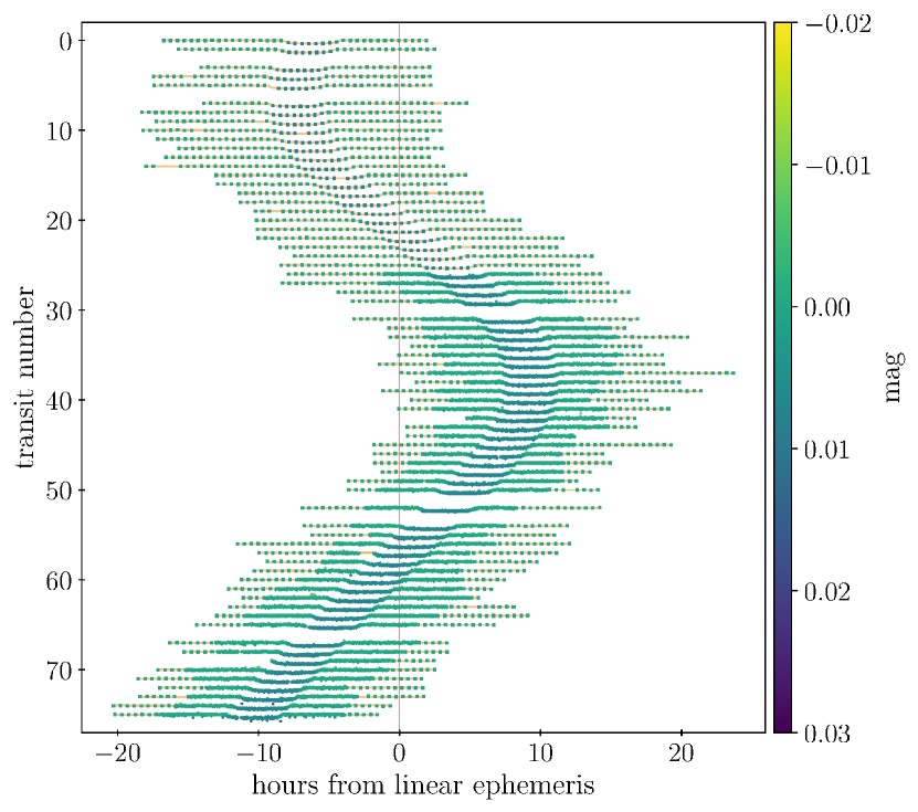
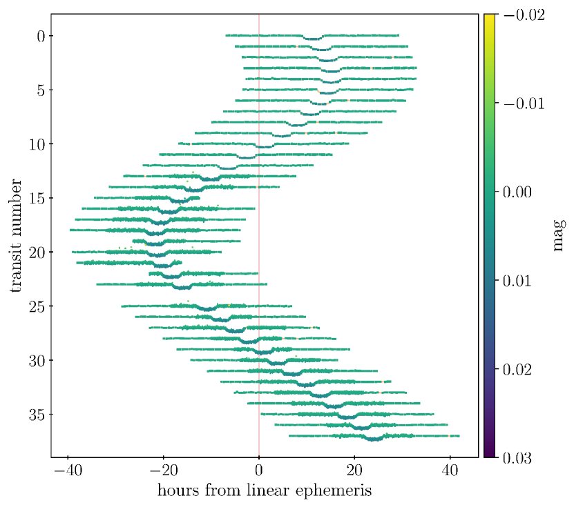
See Fig. 2 and 3 for the river plots of planet b and c, respectively, showing the data and the computed model of each transit in LC and SC and the TTV effect with respect to a linear ephemeris.

As final parameters from the light curve analysis we decided to use the mean between the SC and LC median values of the merged posteriors; we associated as lower uncertainty the lower value between the SC and LC and the greater values for the upper uncertainty. The results are summarised in Table 2.

Figure 2: River plot for Kepler-9b: the LC (and SC when available) of each transit has been plotted with colour code depending on the normalised magnitude (transit with darker colour, best-fit model in orange). The light curves are sorted vertically by each epoch (or transit number with respect to a reference time) as function of the phase (in hours) with respect to a linear ephemeris (vertical line at zero) showing the TTV effect.

Figure 3: Same as Fig. 2, but for Kepler-9c.

5 Orbital parameters from dynamical analysis

We extract from the LC and SC analysis the central time, $T_{0}$, and the total duration, $T_{14}$ (defined as the difference between fourth and first contact time and computed with equation 30 in Kipping, 2010), of each transit; we kept the time and duration from SC when present, otherwise we used the analysis of the LC. We assigned as symmetric errors of $T_{0}$s and $T_{14}$s the maximum between the lower and upper value of the HDI. The measured central time and duration from each transit, in SC or LC mode, are available in Table 4.

For each planet, we used TRADES to fit the following parameters: the mass of the planet in units of stellar mass, $M_{\mathrm{p}}/M_{\star}$, the planetary period $P_{\mathrm{p}}$, the eccentricity vector components $\sqrt{e_{\mathrm{p}}}\cos(\omega_{\mathrm{p}})$ and $\sqrt{e_{\mathrm{p}}}\sin(\omega_{\mathrm{p}})$, where $e_{\mathrm{p}}$ is the eccentricity and $\omega_{\mathrm{p}}$ the argument of pericentre of the planet, the inclination vector components $i\cos(\Omega_{\mathrm{p}})$ and $i\sin(\Omega_{\mathrm{p}})$, where $i$ is the orbital inclination and $\Omega_{\mathrm{p}}$ the longitude of ascending node, and the mean longitude of the planet $\lambda_{\mathrm{p}}$, defined as the sum of the argument of pericentre, the longitude of the ascending node, and the mean anomaly $\mathcal{M}_{\mathrm{p}}$. All the dynamical parameters are computed at the epoch of reference BJD${}_{\textrm{TDB}}=2455088.212$.

We used uniform priors with broad but physically motivated boundaries: planetary periods are constrained within two days of the value of the linear ephemeris, and the mass of the planets, $M_{\mathrm{p}}$, are bounded to less than $2\,M_{\textrm{Jup}}$. We defined the reference coordinate system as described in Winn (2010), therefore Kepler-9b has fixed $\Omega_{\textrm{b}}$ to $180\degr$, effectively reducing the inclination vector of planet b to $i_{\textrm{b}}$. All other parameters have been fixed to the values determined in section 4, e. g., stellar and planetary radius.

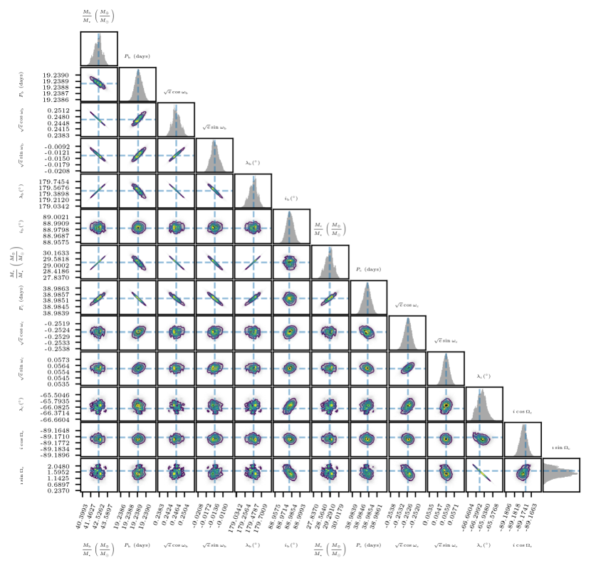
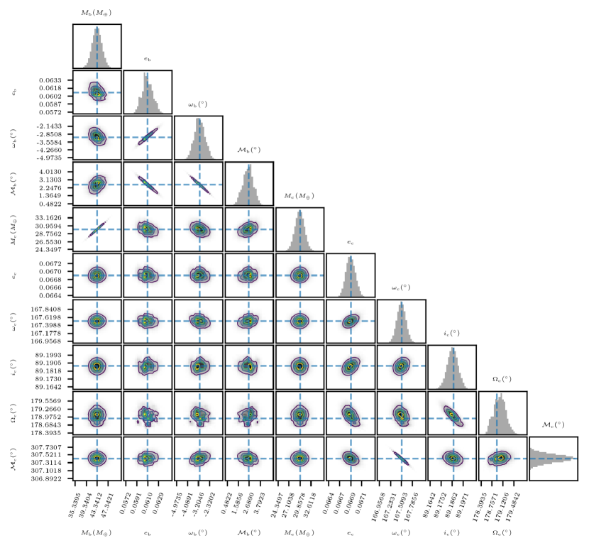
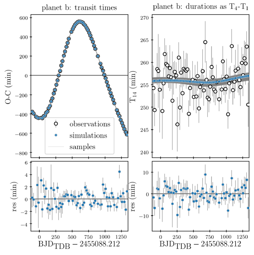
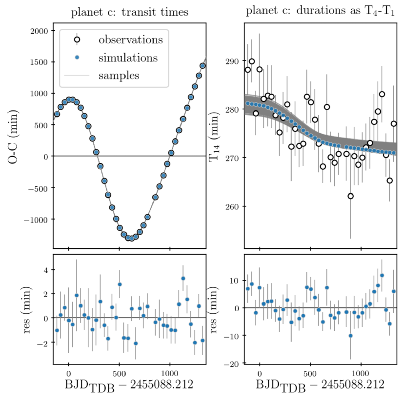
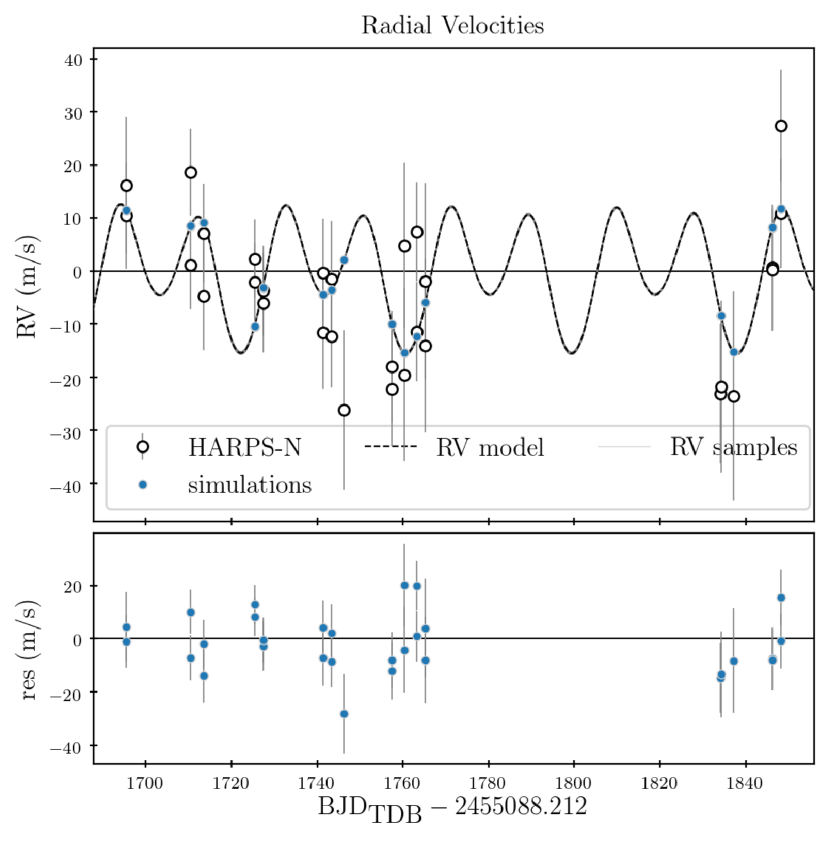
We used an updated version of TRADES that allows us to fit $T_{0}$s and $T_{14}$s simultaneously during the planetary orbit integration and performs a Bayesian analysis with the emcee package; we used the same form of the loglikelihood, $\ln{\mathcal{L}}$, introduced in Malavolta et al. (2017a). Although TRADES can also fit the observed RVs as well, we did not include the HARPS-N data at this stage of the analysis because we wanted to use those observations as an independent check of the TTV-derived solution. We ran a simulation with 200 walkers, 200000 steps, and we discarded the first 50000 steps as burn-in. The initial walkers have been generated from a neighbourhood of the solution from B14. As in the previous section we checked for GR statistics and we obtained the final posterior distribution after the chains had been thinned with a factor of 100; the correlation plots of the posterior distributions of the fitted and derived parameters are shown in Fig 4 and 5, respectively. We computed the final best-fit parameter set as the MLE (and HDI) of the posterior distribution; see the summary of the best-fit parameters in Table 3 and how they reproduce the observed $T_{0}$ and $T_{14}$ data for Kepler-9b and Kepler-9c in Fig. 6 and 7, respectively. Figure 8 shows how the new solution with the newly derived parameters fits the RV observations.

The final solution confirmed the masses and the orbital parameters found in B14.

We also tested a parameter search fixing the inclination to the value from the LC analysis and the longitude of node to $180\degr$, for both planets. In this case the best-fit model found compatible masses but it did not reproduce the trend of the $T_{14}$ data and the final Bayesian Information Criteria was higher.

Figure 4: Correlation plot of the fitted parameters. The MLE solution has been shown as a dashed blue line.

Figure 5: Same as in Fig. 4, but for derived parameters.

Figure 6: O-C (upper-left panel) where O and C mean observed and calculated transit times, respectively and duration (upper-right panel) plots with residuals (lower panels) for the best fit solution for Kepler-9b. Grey lines represent 1000 realisations obtained by randomly selecting sets of parameters from the posterior distributions.

Figure 7: Same as Fig. 6, but for Kepler-9c.

Figure 8: Kepler-9 RV plot (observed RVs as black-open circles) for best fit solution (blue-filled circles). The RV model of the best-fit solution covering the full integration time has been plotted as a black-dashed line. We plotted 1000 realisations (as grey lines) of the model from the posterior distribution, but they all lie too close to the best-fit RV model to be distinguishable from it.

Table 3: Table summarising the dynamical fit solution. Parameter values as the maximum likelihood estimation (MLE) and HDI at $68.27\%$ equivalent. Dynamical parameters are computed at the epoch of reference BJD${}_{\textrm{TDB}}\,2455088.212$.

parameter	Kepler-9b	Kepler-9c
fitted dynamical model
$M_{\mathrm{p}}/M_{\star}$	$0.000128_{-0.000002}^{+0.000001}$	$0.000088_{-0.000001}^{+0.000001}$
$P_{\mathrm{p}}$ (day)	$19.23891_{-0.00006}^{+0.00006}$	$38.9853_{-0.0003}^{+0.0003}$
$\sqrt{e}\cos(\omega_{\mathrm{p}})$	$0.24651_{-0.0027}^{+0.0021}$	$-0.2526_{-0.0003}^{+0.0003}$
$\sqrt{e}\sin(\omega_{\mathrm{p}})$	$-0.014_{-0.002}^{+0.002}$	$0.0559_{-0.0005}^{+0.0005}$
$i$ $(\degr)$	$88.982_{-0.005}^{+0.007}$	–
$i\cos(\Omega_{\mathrm{p}})$	–	$-89.172_{-0.005}^{+0.002}$
$i\sin(\Omega_{\mathrm{p}})$	–	$1.7_{-0.5}^{+0.2}$
$\lambda_{\mathrm{p}}$ $(\degr)^{\textrm{(a)}}$	$179.49_{-0.11}^{+0.15}$	$293.9_{-0.1}^{+0.3}$
derived dynamical model
$M_{\mathrm{p}}$ $(M_{\oplus})$	$43.4_{-2.0}^{+1.6}$	$29.9_{-1.3}^{+1.1}$
$\rho_{\mathrm{p}}$ (g/cm3)	$0.42_{-0.09}^{+0.06}$	$0.31_{-0.06}^{+0.05}$
$e_{\mathrm{p}}$	$0.0609_{-0.0013}^{+0.0010}$	$0.06691_{-0.00012}^{+0.00010}$
$\omega_{\mathrm{p}}$ $(\degr)$	$357.0_{-0.4}^{+0.5}$	$167.5_{-0.1}^{+0.1}$
$\mathcal{M}_{\mathrm{p}}$ $(\degr)$	$2.6_{-0.6}^{+0.5}$	$307.4_{-0.1}^{+0.1}$
$i$ $(\degr)$	–	$89.188_{-0.006}^{+0.005}$
$\Omega_{\mathrm{p}}$ $(\degr)$	$180.$ (fixed)	$179.0_{-0.1}^{+0.3}$
dynamical model $\chi^{2}_{\textrm{r}}$ (dof$=230$)	1.16
${}^{\textrm{(a)}}$ $\lambda_{\mathrm{p}}$ is the mean longitude of the planet, defined as $\lambda_{\mathrm{p}}=\Omega_{\mathrm{p}}+\omega_{\mathrm{p}}+\mathcal{M}_{\mathrm{p}}$.

6 Comparison of literature solutions with RVs

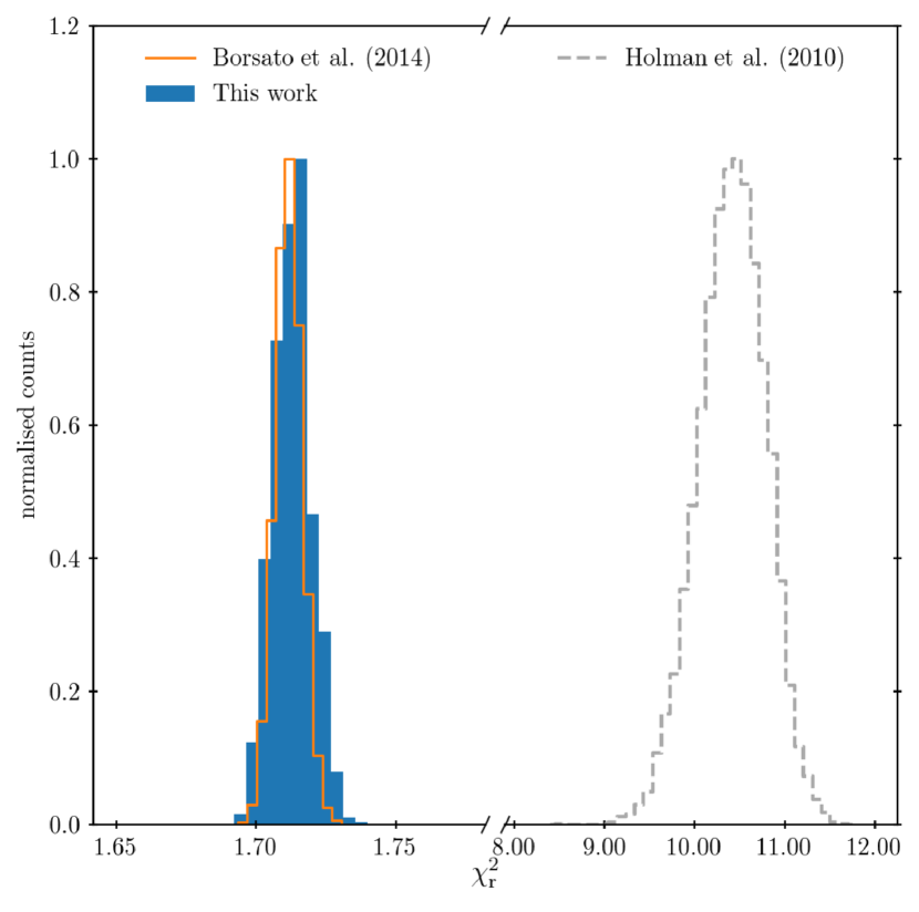
We propagated the solution of H10 and B14 to the epochs of our RVs using the dynamical integrator embedded in TRADES (Borsato et al., 2014). For consistency, we used the stellar masses of the two respective papers. For each solution we generated 10000 sets by varying each parameter of a quantity randomly extracted from a Gaussian distribution with variance equal to the errors listed in Table 3. We then computed the $\chi^{2}_{\textrm{r}}$ of the RVs for each set of orbital parameters. In both cases we have only one free parameter, i. e., the systemic RV of the target, $\gamma$, since all the other parameters have been determined independently of our RV dataset. We can therefore use the $\chi^{2}_{\textrm{r}}$ to select which solution better reproduces our measurements. We select 10000 sets of parameters from the posterior distribution computed in Sec. 5 and compute the $\chi^{2}_{\textrm{r}}$. The distributions of the samples from B14 and this paper overlap each other and they are centred at $\chi^{2}_{\textrm{r}}=1.71$, while the H10 distribution has a higher $\chi^{2}_{\textrm{r}}$ of about 10.5 (see Fig. 9), i. e., the solutions obtained using the $T_{0}$ alone compare well with those from the HARPS-N RVs, and do not depend on the exact number of transits involved in the analysis.

In our analysis we did not include the six Keck/HIRES observations gathered by H10, since their apparent discrepancy with the TTV solutions presented by B14 and following works was what motivated us obtaining new RVs with HARPS-N. While our RV dataset is well described by the TTV solutions presented in B14 and in this work, we still do not have an explanation for the inconsistency with the previous RVs from H10. We note, however, that it is not the first time that a few, sparse Keck/HIRES RVs are in disagreement with a larger RV dataset obtained with HARPS-N (e. g., Sozzetti et al., 2015). Given the observational strategy we employed, the large number of RVs, and the inclusion of possible source of contamination from the Moon, we believe that our dataset is more suitable to confirm or disprove the possible disagreement between TTV and RVs methods.

Figure 9: Histograms of the $\chi^{2}_{\textrm{r}}$ from the RV of the 10000 simulations for the three different solutions: H10 from (Holman et al., 2010), B14 from (Borsato et al., 2014), and from the posterior distribution of this work.

7 Discussion and Conclusions

The apparent disagreement in the distribution of planets in the mass-radius diagram between masses obtained from TTV modelling and masses derived from RVs has been a long-standing problem in the exoplanet community (see Malavolta et al. 2017a for a review of the most interesting cases). The Kepler-9 system is the first system characterised with TTV, and the already low densities of the planets as determined in the discovery paper by Holman et al. (2010) have been further decreased in subsequent analysis by Borsato et al. (2014). Consequently, we selected this system as a proxy to compare RV and TTV masses measurements.

A differential comparison between the predicted RVs from H10 and B14 allowed us to set up the best observational strategy to be carried out with HARPS-N in order to independently confirm the true nature of the Kepler-9 planets and to overcome the fact that the faintness of the star would make a 5-$\sigma$ detection unfeasible. Additionally, we performed an independent analysis of the full Kepler light-curve in order to compare the observed RVs with the prediction of the most precise orbital model that could be obtained from TTVs. In our analysis we also included refined stellar parameters that take into account the precise parallax measurement provided by Gaia DR2, and both literature and newly derived photospheric parameters for the star.

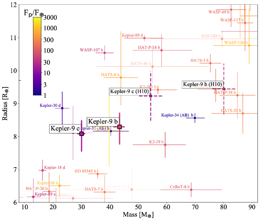
The fit of the whole Kepler data-set confirmed the masses, and hence the densities (see Table 3), originally found by B14. Our mass values are also well consistent with those in the recent work by Freudenthal et al. (2018), meaning that with a dynamical model we have been able to obtain masses with the same precision as the more computationally expensive photodynamical model, even when using space-borne photometry alone. Our analysis places Kepler-9b and c in the mass-radius region of super-Neptunes / inflated sub-Saturns together with other planets recently discovered that also have precise RV-derived masses, such as WASP-139b (Hellier et al., 2017), K2-24c (Dai et al., 2016), K2-39b (Van Eylen et al., 2016) and HATS-8b (Bayliss et al., 2015), as can be seen in Figure 10.

The observed HARPS-N RVs noticeably agree with the model of this paper (and B14) with a $\chi^{2}_{\textrm{r}}$ of 1.71, but are not consistent with the solution from H10 ($\chi^{2}_{\textrm{r}}\sim 10.5$). The high value of the masses found by H10 is ascribable to the very short baseline of the photometric data and due to a possible underestimation of the HIRES RV uncertainties.

The Kepler mission has shown the power of the TTV method to determine the planetary nature of candidates in multiple systems and to characterise the orbital and physical parameters of the exoplanets. The lack of bright stars hosting multiple-planet systems showing TTV in the Kepler field did not allow for high precision RV observation in order to confirm or rule out the mass determination discrepancy. With the advent of the TESS (Ricker et al., 2014) and PLATO (Rauer et al., 2014) missions we will be able to measure the masses of many planets around bright stars with both the TTV and the RV methods allowing us to further investigate the level of consistency in planet parameters between the two methods, or the presence of any bias in the solutions coming from the two techniques.

Figure 10: Mass-Radius plot for Kepler-9b and c. Results from H10 are included for comparisons. Planets with mass determination with uncertainties greater than 20% are shaded accordingly. Planets are color-coded according to their incident flux. Data obtained from exoplanet.eu on October 2018.

Appendix A Time of transit and durations

Central time ($T_{0}$) and duration $T_{14}$ with corresponding error obtained from the fit of each transit, as described in section 5.

Table 4: Transit times and durations as described in section 5. Full table available in electronic form.

Transit number	$T_{0}$	$\sigma_{T_{0}}$	$T_{14}$	$\sigma_{T_{14}}$	SC/LC
${}^{\textrm{(a)}}$	(KBJD${}_{\textrm{TDB}}^{\textrm{(b)}}$)	(min)	(min)	(min)
Kepler-9b
0	144.24992	1.6	254.3	5.0	LC
1	163.48362	1.1	249.4	3.6	LC
3	201.95379	1.2	258.5	3.6	LC
…	…	…	…	…
Kepler-9c
0	136.30647	1.2	288.2	5.2	LC
1	175.33153	1.9	289.9	4.4	LC
2	214.33540	1.1	279.2	4.6	LC
…	…	…	…	…

${}^{\textrm{(a)}}$ Transit number computed with respect to the linear ephemeris in Table 2.

${}^{\textrm{(b)}}$ BJD${}_{\textrm{TDB}}-2454833.0$.

Appendix B Radial Velocity measurements with HARPS-N.

Radial Velocity with corresponding errors obtained with HARPS-N facility.

Table 5: HARPS-N RVs.

Time	RV	$\sigma_{\textrm{RV}}$
(BJD${}_{\textrm{TDB}}$)	(m s-1)	(m s-1)
2456783.60953	2353.88	12.88
2456783.63028	2348.14	10.00
2456798.63783	2338.88	8.42
2456798.66056	2356.35	8.23
2456801.65029	2344.83	9.25
2456801.66955	2333.04	10.26
2456813.53960	2340.04	7.38
2456813.56188	2335.65	7.33
2456815.54510	2331.71	9.40
2456815.56727	2334.02	8.52
2456829.53712	2337.37	10.28
2456829.55869	2326.08	10.58
2456831.58087	2325.38	9.56
2456831.60226	2336.21	11.00
2456834.50224	2311.57	15.00
2456845.67515	2319.74	10.48
2456845.69621	2315.50	10.85
2456848.44839	2342.51	15.55
2456848.46990	2318.14	16.26
2456851.45439	2345.14	9.33
2456851.47538	2326.24	9.37
2456853.45667	2323.64	16.36
2456853.47773	2335.83	18.50
2456922.38581	2314.59	13.09
2456922.40526	2315.97	16.20
2456925.37421	2314.17	19.65
2456934.36631	2338.37	11.78
2456934.38747	2337.96	11.48
2456936.46863	2365.09	10.49
2456936.49021	2348.56	10.31

References

- Agol et al. (2005) Agol E., Steffen J., Sari R., Clarkson W., 2005, MNRAS, 359, 567
- Barros et al. (2015) Barros S. C. C. et al., 2015, MNRAS, 454, 4267
- Bayliss et al. (2015) Bayliss D. et al., 2015, AJ, 150, 49
- Becker et al. (2015) Becker J. C., Vanderburg A., Adams F. C., Rappaport S. A., Schwengeler H. M., 2015, ApJ, 812, L18
- Borsato et al. (2014) Borsato L., Marzari F., Nascimbeni V., Piotto G., Granata V., Bedin L. R., Malavolta L., 2014, A&A, 571, A38
- Borucki et al. (2011) Borucki W. J. et al., 2011, ApJ, 736, 19
- Buchhave et al. (2014) Buchhave L. A. et al., 2014, Nature, 509, 593
- Buchhave et al. (2012) Buchhave L. A. et al., 2012, Nature, 486, 375
- Choi et al. (2016) Choi J., Dotter A., Conroy C., Cantiello M., Paxton B., Johnson B. D., 2016, ApJ, 823, 102
- Cochran et al. (2011) Cochran W. D. et al., 2011, ApJS, 197, 7
- Cutri et al. (2003) Cutri R. M. et al., 2003, VizieR Online Data Catalog, 2246
- Dai et al. (2016) Dai F. et al., 2016, ApJ, 823, 115
- Dotter (2016) Dotter A., 2016, ApJS, 222, 8
- Dotter et al. (2008) Dotter A., Chaboyer B., Jevremović D., Kostov V., Baron E., Ferguson J. W., 2008, ApJS, 178, 89
- Eastman, Gaudi & Agol (2013) Eastman J., Gaudi B. S., Agol E., 2013, PASP, 125, 83
- Feroz & Hobson (2008) Feroz F., Hobson M. P., 2008, MNRAS, 384, 449
- Feroz, Hobson & Bridges (2009) Feroz F., Hobson M. P., Bridges M., 2009, MNRAS, 398, 1601
- Feroz et al. (2013) Feroz F., Hobson M. P., Cameron E., Pettitt A. N., 2013, ArXiv e-prints
- Foreman-Mackey et al. (2013) Foreman-Mackey D., Hogg D. W., Lang D., Goodman J., 2013, PASP, 125, 306
- Freudenthal et al. (2018) Freudenthal J. et al., 2018, A&A, 618, A41
- Gaia Collaboration et al. (2018) Gaia Collaboration, Brown A. G. A., Vallenari A., Prusti T., de Bruijne J. H. J., Babusiaux C., Bailer-Jones C. A. L., 2018, ArXiv e-prints
- Gaia Collaboration et al. (2016) Gaia Collaboration et al., 2016, A&A, 595, A1
- Gelman & Rubin (1992) Gelman A., Rubin D. B., 1992, Statistical Science, 7, 457
- Goodman & Weare (2010) Goodman J., Weare J., 2010, Communications in Applied Mathematics and Computational Science, Vol. 5, No. 1, p. 65-80, 2010, 5, 65
- Hellier et al. (2017) Hellier C. et al., 2017, MNRAS, 465, 3693
- Holman et al. (2010) Holman M. J. et al., 2010, Science, 330, 51
- Holman & Murray (2005) Holman M. J., Murray N. W., 2005, Science, 307, 1288
- Huber et al. (2014) Huber D. et al., 2014, ApJS, 211, 2
- Jontof-Hutter et al. (2016) Jontof-Hutter D. et al., 2016, ApJ, 820, 39
- Kipping (2010) Kipping D. M., 2010, MNRAS, 407, 301
- Kipping (2013) Kipping D. M., 2013, MNRAS, 435, 2152
- Kreidberg (2015) Kreidberg L., 2015, PASP, 127, 1161
- Lissauer et al. (2011) Lissauer J. J. et al., 2011, Nature, 470, 53
- Lovis et al. (2011) Lovis C. et al., 2011, ArXiv e-prints
- Malavolta et al. (2017a) Malavolta L. et al., 2017a, AJ, 153, 224
- Malavolta et al. (2017b) Malavolta L., Lovis C., Pepe F., Sneden C., Udry S., 2017b, MNRAS, 469, 3965
- Malavolta et al. (2018) Malavolta L. et al., 2018, AJ, 155, 107
- Masuda et al. (2013) Masuda K., Hirano T., Taruya A., Nagasawa M., Suto Y., 2013, ApJ, 778, 185
- Mills & Mazeh (2017) Mills S. M., Mazeh T., 2017, ApJ, 839, L8
- Mortier et al. (2014) Mortier A., Sousa S. G., Adibekyan V. Z., Brandão I. M., Santos N. C., 2014, A&A, 572, A95
- Morton (2015) Morton T. D., 2015, isochrones: Stellar model grid package. Astrophysics Source Code Library
- Nespral et al. (2017) Nespral D. et al., 2017, A&A, 601, A128
- Osborn et al. (2017) Osborn H. P. et al., 2017, A&A, 604, A19
- Pace (2013) Pace G., 2013, A&A, 551, L8
- Paxton et al. (2011) Paxton B., Bildsten L., Dotter A., Herwig F., Lesaffre P., Timmes F., 2011, ApJS, 192, 3
- Petigura et al. (2017) Petigura E. A. et al., 2017, AJ, 154, 107
- Rauer et al. (2014) Rauer H. et al., 2014, Experimental Astronomy, 38, 249
- Ricker et al. (2014) Ricker G. R. et al., 2014, in Proc. SPIE, Vol. 9143, Space Telescopes and Instrumentation 2014: Optical, Infrared, and Millimeter Wave, p. 914320
- Skrutskie et al. (2006) Skrutskie M. F. et al., 2006, AJ, 131, 1163
- Sneden (1973) Sneden C., 1973, ApJ, 184, 839
- Sousa et al. (2015) Sousa S. G., Santos N. C., Adibekyan V., Delgado-Mena E., Israelian G., 2015, A&A, 577, A67
- Sozzetti et al. (2015) Sozzetti A. et al., 2015, A&A, 575, L15
- Stassun & Torres (2018) Stassun K. G., Torres G., 2018, ApJ, 862, 61
- Steffen (2016) Steffen J. H., 2016, MNRAS, 457, 4384
- Storn & Price (1997) Storn R., Price K., 1997, Journal of Global Optimization, 11, 341
- Torres et al. (2011) Torres G. et al., 2011, ApJ, 727, 24
- Van Eylen et al. (2016) Van Eylen V. et al., 2016, AJ, 152, 143
- von Essen et al. (2018) von Essen C. et al., 2018, ArXiv e-prints, arXiv:1801.06191
- Wang et al. (2018) Wang S., Addison B., Fischer D. A., Brewer J. M., Isaacson H., Howard A. W., Laughlin G., 2018, AJ, 155, 70
- Weiss et al. (2016) Weiss L. M. et al., 2016, ArXiv e-prints
- Weiss & Marcy (2014) Weiss L. M., Marcy G. W., 2014, ApJ, 783, L6
- Weiss et al. (2013) Weiss L. M. et al., 2013, ApJ, 768, 14
- Winn (2010) Winn J. N., 2010, ArXiv e-prints