AIMS - A new tool for stellar parameter determinations using asteroseismic constraints

Abstract

A key aspect in the determination of stellar properties is the comparison of observational constraints with predictions from stellar models. Asteroseismic Inference on a Massive Scale (AIMS) is an open source code that uses Bayesian statistics and a Markov Chain Monte Carlo approach to find a representative set of models that reproduce a given set of classical and asteroseismic constraints. These models are obtained by interpolation on a pre-calculated grid, thereby increasing computational efficiency. We test the accuracy of the different operational modes within AIMS for grids of stellar models computed with the Liège stellar evolution code (main sequence and red giants) and compare the results to those from another asteroseismic analysis pipeline, PARAM. Moreover, using artificial inputs generated from models within the grid (assuming the models to be correct), we focus on the impact on the precision of the code when considering different combinations of observational constraints (individual mode frequencies, period spacings, parallaxes, photospheric constraints,…). Our tests show the absolute limitations of precision on parameter inferences using synthetic data with AIMS, and the consistency of the code with expected parameter uncertainty distributions. Interpolation testing highlights the significance of the underlying physics to the analysis performance of AIMS and provides caution as to the upper limits in parameter step size. All tests demonstrate the flexibility and capability of AIMS as an analysis tool and its potential to perform accurate ensemble analysis with current and future asteroseismic data yields.

1 Introduction

At present, asteroseismic supporting space missions in operation and ground-based networks (TESS, Ricker et al. 2015; SONG, Andersen et al. 2014; Grundahl et al. 2017) or retired missions (CoRoT, Baglin et al. 2006; CoRot Team 2016; Kepler, Borucki et al. 2010; K2, Howell et al. 2014) have generated high quality data for large ensembles of stars. Further missions are also in preparation (PLATO, Rauer et al. 2014). In order to model these stars, we need pipelines that can efficiently compare observations and models. They must be stable, robust and fast to deal with the current volume of data and the subsequent increases expected in the future.

Often, inferred pipeline properties rely on simple scaling relations of the large frequency separation ($\Delta\nu$) and the frequency of maximum oscillation power ($\nu_{\rm{max}}$) (Kjeldsen & Bedding, 1995). Though quick and simple to use, more robust estimations can be made when, for example, the average large frequency separations from model predicted radial mode frequencies and the use of gravity mode period spacings are considered in the parameter determinations (see Rodrigues et al. 2017; Serenelli et al. 2017). Though an improvement, these still do not exploit all of the information the individual modes contain, e.g., presence of acoustic glitches (Vorontsov, 1988; Gough, 1990; Miglio et al., 2010; Pérez Hernández et al., 2016; Verma et al., 2017) and long term internal structure changes from curvature of the large frequency separation (Hekker & Christensen-Dalsgaard, 2017; Mosser et al., 2012).

Multiple asteroseismic modelling techniques have been developed with the objective to fully exploit seismic information (Guenther & Brown 2004, Miglio & Montalbán 2005, Bazot et al. 2008, Metcalfe et al. 2009, Gruberbauer et al. 2012, PARAM (da Silva et al., 2006; Rodrigues et al., 2014, 2017); see the KAGES (Silva Aguirre et al., 2015; Davies et al., 2016) and LEGACY (Lund et al., 2017; Silva Aguirre et al., 2017) projects for further pipelines).

The use of individual mode frequencies as constraints to the analysis, increases significantly both the precision and accuracy of the inferred masses, radii and age for both main sequence (e.g. Lebreton & Goupil 2014 for a recent review, Reese et al. 2016 for tests using artificial data, or results based on Kepler’s best data sets by Silva Aguirre et al. 2017) and red giant stars (Huber et al., 2013; Lillo-Box et al., 2014; Pérez Hernández et al., 2016; Li et al., 2018). Improving the use of seismic information will lead to more precise global stellar properties and allow for testing aspects of the micro- and macro-physics which are currently poorly constrained.

We present here the stellar modelling pipeline, AIMS (Asteroseismic Inference on a Massive Scale, Reese 2016; Lund & Reese 2018). AIMS is a pipeline designed to process the measured individual acoustic oscillation frequencies of stars coupled with classical, spectroscopic or interferometric constraints to provide a powerful diagnostic tool for the determination of stellar properties. Much like Bazot et al. (2008), Gruberbauer et al. (2012), and BASTA (Silva Aguirre et al., 2015), AIMS uses a Bayesian approach. Bazot et al. (2008) implements an on-the fly model calculation with an MCMC algorithm to produce a representative sample of model parameters. This leads to a higher accuracy but at a significant computational cost, whereas the remaining codes use pre-computed grids (faster calculation time). Gruberbauer et al. (2012) and BASTA then evaluate probability distribution functions by scanning the grid. Like Bazot et al. (2008), AIMS also uses an MCMC algorithm, but what is unique is that it is combined with model interpolation. This provides a compromise between accuracy and efficiency.

This paper details the capabilities and potential of AIMS and its applicability within the scientific community. The paper is set out as follows: Section 2 describes the functionality of the code and section 3 describes the input grids containing the models used in the analysis. Sections 4 and 5 discuss the results of the various interpolation tests on the grids and the performance of the program in analysing artificial and real data. Finally, a comparison of the performance of AIMS using different combinations of asteroseismic and classical constraints is given in section 6. The results of these tests are discussed with a summary of the work in section 7.

2 AIMS

AIMS uses Bayesian statistics and a Markov-Chain-Monte-Carlo (MCMC) algorithm (emcee, Foreman-Mackey et al. 2013) to select models representative of the input data by interpolating in a pre-defined grid. The combination of these techniques allows for an efficient, comprehensive search of the parameter space defined by the grid parameters. User-defined priors and the likelihood function resulting from the input constraints shape the exploration of the parameter space. AIMS initialises the grid search in the region of a set of models with the highest posterior probability. This increases the efficiency of the parameter space exploration, which in turn helps the MCMC algorithm converge faster.

The program itself has three modes of functionality: binary grid generation; interpolation testing; and stellar parameter characterisation. The performance and capabilities of interpolation mechanism and stellar parameter determination are tested here. Information on the other functions can be found in the supporting documentation.

To determine stellar parameters in a Bayesian manner, an affine invariant ensemble Markov chain Monte Carlo (MCMC) sampler (Goodman & Weare, 2010) is implemented via the Python package emcee developed by Foreman-Mackey et al. (2013). For a given data file, the user can employ so-called walkers that are initiated in a tightball configuration (optional), uniformly distributing the walkers within a sphere centred on an initial estimation of the most probable grid model. If tightball is not selected, the walkers are initiated through the sampling of model parameter priors. The step number for the walkers can be user defined. Parallel tempering is available with the option to define the number of temperatures, and the MCMC chains can be thinned.

To determine the properties of targets falling between grid points defined by the evolutionary tracks, AIMS uses a two step interpolation procedure of the model parameters:

1. Linear interpolation in the chosen evolutionary parameter along a track.

2. Interpolation between tracks.

This method allows for greater control over the evolutionary parameter (prevention of exceeding the boundaries of evolutionary tracks) and attempts to achieve greater accuracy as consecutive models on an evolutionary sequence are not expected to change significantly. AIMS includes an accuracy test of the interpolation procedure and an additional program is joined to AIMS to visualise these results as a function of the global grid parameters.

The linear interpolation along a track can be modified to use various evolutionary parameters. However, only a parameter varying monotonically as a star evolves should be used to prevent any spurious results or unexpected errors within the interpolation. Examples of such variables include the Helium core mass in red giant branch (RGB) stars or the central hydrogen content for main sequence stars (MS).

3 The Grid - CLÉS with LOSC

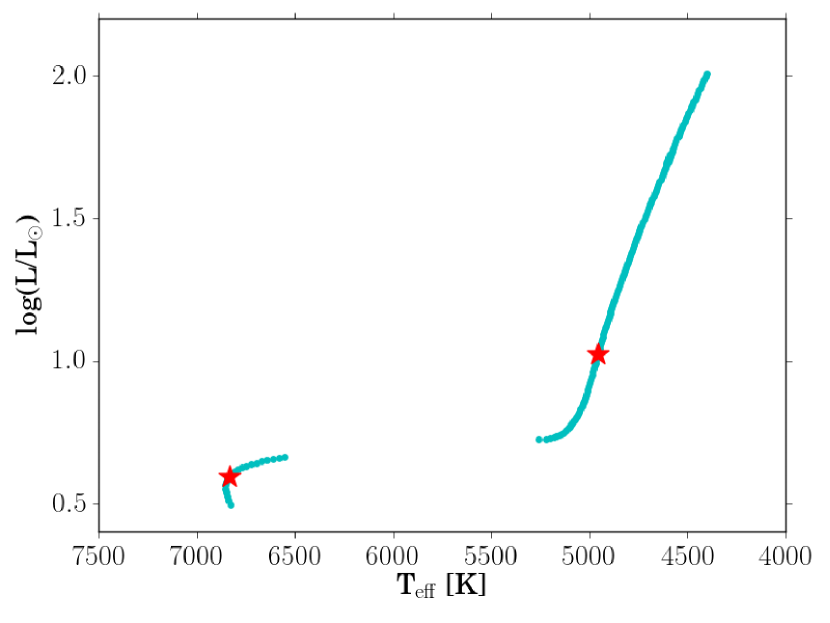
The analysis performed by AIMS is based upon the exploration of a predefined grid of models. In this work, the grid is parametrised by mass (0.75-2.25 M_⊙, in 0.02 M_⊙ increments), initial metallicity ($Z_{\rm{init}}$) and initial hydrogen content ($X_{\rm{init}}$). The range of $X_{\rm{init}}$ and $Z_{\rm{init}}$ values ([Fe/H] values also included for completeness) used can be found in Table 1. Fig. 1 is a Hertzsprung-Russell diagram (HRD) showing the evolutionary tracks calculated for this grid for a given chemical composition. A gap between the MS and sub-giant branch can be observed due to the selection criteria used to split the nominal grid into specific MS and red giant sub grids, which is described in detail later.

Table 1: The values of $X_{\rm{init}}$, $Z_{\rm{init}}$ and [Fe/H] attributed to the CLÉS grid of models.

$X_{\rm{init}}$	$Z_{\rm{init}}$	[Fe/H]
0.691	0.0300	0.25
0.716	0.0175	0.00
0.731	0.0100	-0.25
0.740	0.0057	-0.50
0.745	0.0032	-0.75

The grid contains the evolutionary tracks of theoretical stellar models and their frequencies. Here, we considered $\sim 38000$ models, but larger grids of up to $\sim 1.5$ million models have been used in the past. The models were computed using the CLES (Code Liégeois d’Évolution Stellaire, Scuflaire et al. 2008a) stellar evolution code and the frequencies were generated using the LOSC (Liège Oscillation Code, Scuflaire et al. 2008b) pulsation code. We use the Grevesse & Noels (1993) abundances, nuclear reaction rates of Adelberger et al. (2011), opacities of Iglesias & Rogers (1996) and the FreeEOS equation of state (Irwin, 2012). The mixing-length parameter was kept to a solar calibrated value of $1.67$ and a convective overshoot of $0.05$ times the local pressure scale height was used, assuming instantaneous chemical mixing and the radiative temperature gradient in the overshooting region. Microscopic diffusion was not included in the grid. The border of the convective zones was calculated following the guidelines of Gabriel et al. (2014) to avoid spurious solutions for the evolution of convective cores.

Figure 1: Hertzsprung Russell Diagram displaying the evolutionary tracks found within the CLÉS grid ($X_{\rm{init}}$ = 0.731, $Z_{\rm{init}}$ = 0.0100). The gap between the end of the MS and beginning of the sub-giant branch is due to the Helium core mass fraction selection criterion for the MS and RGB grids.

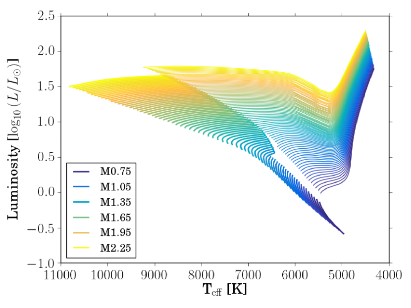
In this work, we used two sub-grids: one for MS and another for RGB stars. We based our criteria on the changes in chemical composition (variations of central hydrogen for the MS, helium core mass for the RGB), effective temperature and $\nu_{\rm{max}}$ values. While AIMS is very versatile in the grids it can use, it should be noted that the tracks must contain a sufficient number of models to ensure an accurate interpolation. On the MS, we included modes with angular degree ($\ell$) values of 0, 1 and 2 whereas the RGB grid only used radial modes ($\ell=0$). This difference stems from intrinsic limitations of AIMS in processing non-radial modes of RGB stars which are highly non-linear. Both grids included radial orders of the frequencies in the range $n=0-30$. It should be noted that the grids were built to test the functionality of the code that we will describe in sections 4 and 5.

4 Interpolation Testing

The objective of AIMS is to carry out precise asteroseismic analyses. Hence, it is paramount to ensure an accurate interpolation of the determined stellar properties to ensure the reliability of the modelling results. Here, we briefly present the interpolation procedure used in AIMS and the tests that can be made to certify accurate and reliable results.

4.1 Interpolation Procedure

AIMS uses a two step interpolation process to explore the regions between models, namely:

1. interpolation between evolutionary tracks

2. interpolation along an evolutionary track

Interpolation between the tracks relies on a multi-dimensional Delaunay tessellation (see Field 1991 and references therein) of the grid parameters excluding age. The tessellation and subsequent interpolation are carried out by python’s scipy.spatial.Delaunay module which is based on the Qhull package (Barber et al., 1996). Using a tessellation approach offers two advantages: the grid does not need to be structured, and fewer tracks (namely $\rm{n}_{\rm{dim}}+1$ as opposed to $2^{\rm{n}_{\rm{dim}}}$, where $\rm{n}_{\rm{dim}}\geq 2$ is the number of dimensions excluding age) are used when interpolating at a given point, accelerating the calculations. During the tessellation, the parameter space is divided into simplices (i.e. triangles in the 2D case, tetrahedra in the 3D case, etc.). For a given point in this space, AIMS searches for the simplex containing it and carries out a linear combination of its vertices (or nodes). The interpolation coefficients correspond to barycentric coordinates provided by scipy.spatial.Delaunay. These coefficients are simply the ratios between the volumes of the reduced simplices where one of the vertices has been replaced by the point where the interpolation is carried out and the volume of the original simplex.

Interpolation along the tracks consists of a linear interpolation in age between the two closest models. Points outside the tracks are rejected, i.e. AIMS does not perform extrapolation. AIMS can either interpolate according to the physical age, or according to an age parameter which has been scaled to go from 0 to 1 along the track (e.g. helium core mass in red giants). This latter option is more robust as it is less likely to lead to extrapolation (and hence model rejection) when the two interpolation steps are combined. Indeed, the point where the interpolation is being carried out only needs to be within the age span of the interpolated track rather than having to lie within the age span of all tracks involved in the interpolation, as illustrated in Fig. 2.

Figure 2: Comparison of physical and scaled age interpolation. In the right panel, only scaled age interpolation works.

The determined coefficients are then used to interpolate the models by linearly combining the global parameters $M$, $X_{0}$ (the initial hydrogen content), $Z_{0}$ (the original metallicity), $T_{\mathrm{eff}}$, and $\rho$ (the mean density). The radius and luminosity are then determined self-consistently from these interpolated parameters using the relations:

$$R=\left(\frac{3M}{4\pi\rho}\right)^{1/3},\qquad L=4\pi\sigma R^{2}T_{\mathrm{eff}}^{4}.$$ (1)

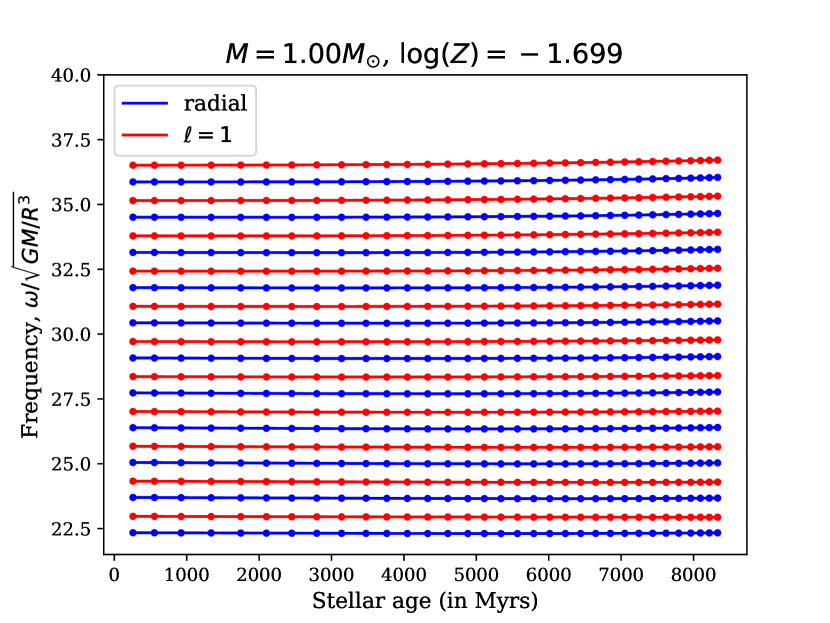
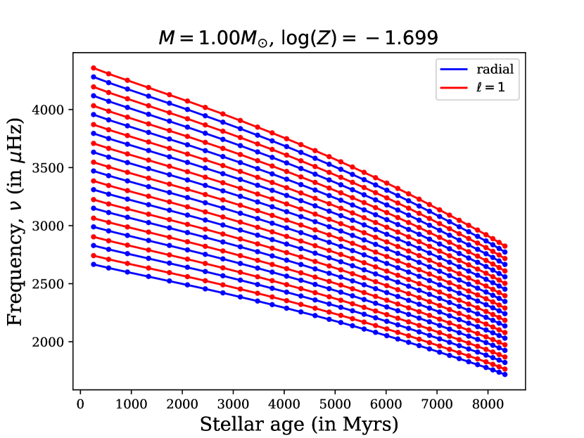
We note that even the constant $\sigma$ is interpolated linearly in case there were any departures from the Stefan-Boltzmann law. Any supplementary user-provided global parameters are interpolated linearly. The mean density is interpolated linearly rather than the radius in order to be consistent with the results from InterpolateModel. Non-dimensional frequencies, $\omega/\sqrt{GM/R^{3}}$, with the same $n$ and $\ell$ identification are interpolated linearly rather than their dimensional counterparts, as they vary much more slowly as a function of stellar parameters, as illustrated in Fig. 3. They are subsequently multiplied by $\sqrt{GM/R^{3}}$, using the interpolated values of $M$ and $R$, in order to remain consistent with the interpolated global parameters. The interested reader is referred to the AIMS documentation for additional information.

Figure 3: Frequencies as a function of stellar age along an evolutionary track. The upper panel corresponds to non-dimensional frequencies and the lower panel to their dimensional counterparts. The symbols correspond frequencies from the non-interpolated models whereas the continuous lines represent the interpolated frequencies.

4.2 Interpolation Results

In this section, we present the tests included in AIMS to check the suitability of the interpolation procedure to fit observational data. We compare the interpolation errors to the typical uncertainties of observed targets found in the literature. On the MS, we used 16-Cyg A, which yields a median frequency uncertainty on the $l=0$ modes of 0.08 $\mu$Hz (-1.097 in log₁₀) and a smallest uncertainty of 0.04 $\mu$Hz (-1.398 in log₁₀). On the RGB, we use KIC4448777, which has a median frequency uncertainty on the $l=0$ modes of 0.018 $\mu$Hz (-1.745 in log₁₀) and a smallest uncertainty of 0.014 $\mu$Hz (-1.854 in log₁₀).

4.3 Interpolation along evolutionary tracks

The evaluation of the interpolation errors along an evolutionary track is made by testing how well both frequencies and global parameters of each model can be recovered from adjacent models at 1 and 2 increments away. Figure 4 shows the RMS average interpolation errors on the frequencies over the range $\nu_{\mathrm{max}}\pm 0.2\nu_{\mathrm{max}}$ for the MS and RGB grids detailed in Section 3. Overall the errors are smaller than the smallest frequency uncertainty of 16-Cyg A over the tested frequency range for both single and double increments. The behaviour of the interpolation error is in line with the expectations for a simple linear interpolation, as it increases by a factor of $\sim 4$. Increased errors are seen between 1.2 and 1.8 $M_{\odot}$ and are linked to the onset of a convective core during the evolution. The results are, however, satisfactory as they are well below the observational error bars.

Figure 4: Average frequency interpolation errors over the range $\nu_{\mathrm{max}}\pm 0.2\nu_{\mathrm{max}}$ along evolutionary tracks for radial modes from the MS grid (left panels) and the RGB grid (right panels). The upper panels use increments of $1$ along the tracks whereas the lower panel corresponds to increments of $2$. The magenta and black contours correspond to the average and smallest error bars of KIC4448777. The average and lowest uncertainties for 16-Cyg A are not shown as they are greater than the uncertainty range shown

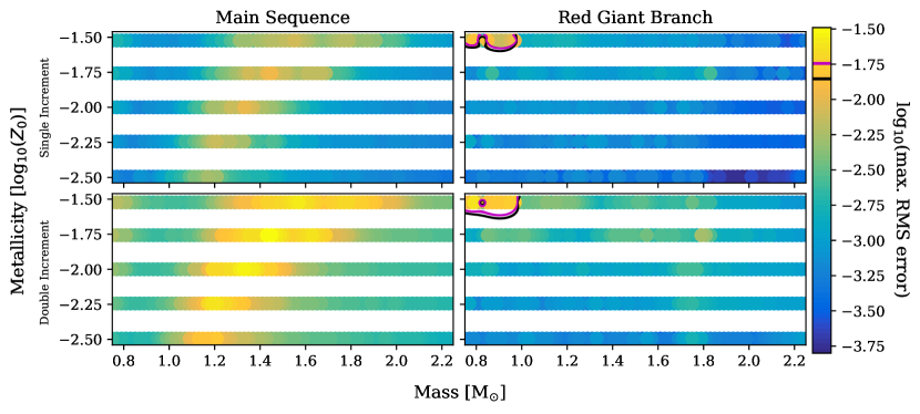
On the RGB, the interpolation errors remain below the smallest and average uncertainties for KIC4448777 apart from a small region at low masses and high metallicities, which represents 2 to $3\,\%$ of the models, as highlighted in the right panels of Fig. 4 by the black and magenta contours respectively. Again, using double increments in the interpolation leads to an increase in line with numerical expectations. While the RGB results may seem worse than for the MS, one must bear in mind the comparatively smaller error thresholds on the RGB. The RGB interpolation errors remain actually smaller than the MS, as shown in Fig. 4 and can of course be reduced by refining the grid.

4.4 Cross Track Interpolation

As a result of the multi-dimensional character of the parameter space and the use of Delaunay tessellation, the approach used to test cross-track interpolation in AIMS is quite different. The grid is partitioned in two sub grids: one to form the simplices for the interpolation and one containing the tracks to be recovered via interpolation. The partition is made randomly to avoid biasing the test towards one of the directions. This, however, means that the models are not always adjacent to the interpolated ones, reducing the representativity with respect to what is done in practice.

Panel (A) of Fig. 5 displays the recovered sub-grid from the MS interpolation. The RMS average interpolation errors are consistent with the MS and RGB values for along track interpolation, but extend to higher values in some regions. These predominately follow the increased error pattern in Fig. 4. Higher uncertainties are expected though, as a greater range of parameter space than normally used is interpolated across. The maximum interpolation errors are the order of the average frequency uncertainty of 16-Cyg A. The errors are acceptable as the values are consistent with average observation uncertainties for interpolations over greater ranges than will be executed during real parameter determination.

Selecting a model from the recovered sub-grid, one can see how well the interpolation has reconstructed the original track. Panel (B) of Fig. 5 shows the recovered 1.47 M_⊙, $X_{\rm{init}}$ = 0.740, $Z_{\rm{init}}$ = 0.0057 track and panel (C) an echelle diagram for the original and interpolated frequencies for a single model. The interpolated temperatures, luminosities and frequencies vary fractionally about the original values, illustrating further the accuracy of the interpolation method.

Figure 5: An example of results achieved recovering a 1.47 M_⊙, $X_{\rm{init}}$ = 0.740, $Z_{\rm{init}}$ = 0.0057 track during interpolation testing: (A) - Colour map of the maximum interpolated frequency uncertainty along each track. Points represent the positions re-interpolated tracks; the red circle shows the position of the track used in part (B). This track has a maximum log₁₀ uncertainty on the interpolated frequencies of -1.990. The red circle highlights the location of the track. Grey points and lines show the triangulation simplices for the interpolation. Red diamonds donte tracks not interpolated due to no triangulation being possible. (B) - Hertzsprung-Russell Diagram showing the original track (blue line), interpolated track (red markers) and the models the track was interpolated from. Models used for interpolation are connected to the respective interpolated models by grey dashed lines and are shifted by 0.5 L_⊙ for additional clarity. The fractional difference residuals in luminosity and $T_{\rm{eff}}$ between the original and interpolated models are shown. The $T_{\rm{eff}}$ residuals have been inflated by a factor of 100. The red circle marks the model used in (C). (C) - An echelle diagram showing the original (blue, closed) and interpolated (orange, open) frequencies for the highlighted model in (B). Full frequency range is shown with diagram modulated by the original model $\Delta\nu$ value. All frequencies have been shifted by 5$\mu$Hz in the x-direction for clarity.

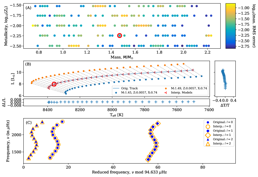
Appendix A.1 shows an example of the RGB grid. The variation in the residuals is minimal, confirming the proper behaviour of the interpolation. In additional tests, some instances show variations from the expected values along sections of the track. These features are largest when interpolating between grid points separated widely in mass (> 0.05 M_⊙) or metallicity, consistent with the regions of increased uncertainty in Fig. 5 outside of the convective onset region.

4.5 Other Parameters

These tests can also be performed for parameters such as mass, radius, luminosity, effective temperature and surface metallicity ratios. The results are not presented here to avoid redundancy but details an be found in Appendix A.2. Again, these tests validated the quality of the grid at both the single and double increment level.

5 Observational Outputs and Constraints

In this section, we present the robustness and accuracy of AIMS in reproducing accurately and precisely stellar parameters. The results presented here illustrate the absolute precision AIMS could achieve for the specific grid used in this study. It should be noted that the performance will depend on the grid and the free parameters included.

5.1 Artificial Data

At first, tests were performed using models from the underlying CLÉS grids. An observation file for a single, randomly selected model containing the artificial frequencies, $T_{\rm{eff}}$, $\nu_{\rm{max}}$, luminosity ($L$) and [Fe/H] values for the track was generated. This track was then removed from the grid. The input file was perturbed 100 times to simulate noise in the data signal. This artificial target was fitted using 100 AIMS runs and the average values from these consecutive fits and their uncertainties were used to determine the degree of success of the procedure.

The asteroseismic constraints selected for use in the analysis were the individual mode frequencies. There are multiple options that can be selected for the seismic constraints, with each having a slightly different effect on the output parameters. Other constraints such as the average $\Delta\nu$ and various frequency separation ratios (r_0,1, r_0,2, r_1,0) could have been used. Using individual mode frequencies gives the smallest uncertainties on the derived parameters, but the final parameter values remain consistent throughout.

One should be cautious though as individual frequencies are not individually unique constraints and can lead to an underestimation of uncertainties. They are also significantly affected by surface effects (this is true of other parameters, e.g. mass, but the changes are more obvious in such cases), at a level such that the precision of the fit is determined by the uncertainties in the surface correction rather than the frequencies (see Buldgen et al. 2018a for examples).

5.1.1 Main Sequence

A 1.27 M_⊙, $Z_{\rm{init}}=$ 0.01 and $X_{\rm{init}}=$ 0.731 MS model with 21 mode frequencies (7 of each of $l=0,1,2$) was selected (see Fig. 6). We used the uncertainty distribution of 16-CygA (Davies et al., 2015) for our artificial target. The magnitude of the uncertainties are of the same order as those used in the “Sun-as-a-star” tests in section 5.2. Uncertainties in [Fe/H] and $T_{\rm{eff}}$ were of order 0.1 dex and 80 K respectively. The uncertainty on the luminosity was selected to be of order 3$\%$ based on Gaia (Gaia Collaboration et al., 2018) parallaxes, with a large proportion of the uncertainty due to the applied bolometric corrections (Torres, 2010; Casagrande & VandenBerg, 2014, 2018). No surface effects were used for both the artificial target and the seismic modelling.

Figure 6: HR diagram showing the evolution of the 1.27 M_⊙, $Z_{\rm{init}}=$ 0.0100, $X_{\rm{init}}=$ 0.731 track. The red stars indicate the positions of the models selected for the artificial data analysis on the MS and RGB. Models prior to the zero-age-main-sequence (ZAMS) have been removed for clarity and final grid selection criteria have been applied.

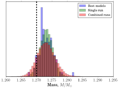
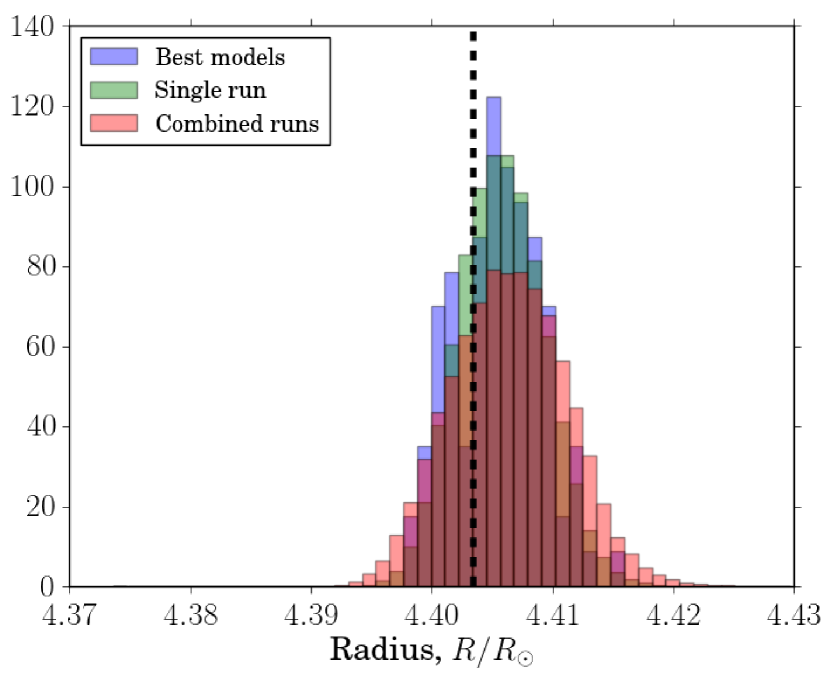
The values and uncertainties of the unperturbed model, the 100 realisations (combined runs) and the best models determined by the MCMC process for each of the perturbed runs were compared to the real values of the model. Examples of the PDF distributions for the mass and radius for each of the 3 trials are shown in Fig. 7.

Figure 7: The mass (left) and radius (right) PDF distributions for RGB the single model (green), 100 realisations (red) and best models from the MCMC runs (blue). The model mass and radii are 1.27 M_⊙ and 1.414 R_⊙, indicated by the vertical black, dotted line.

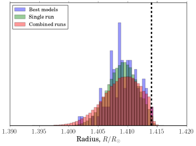The evidence from Fig. 7 indicates that the three different statistics agree reasonably well about a common value. The peaks of the distributions are not centred precisely about the expected values (black vertical lines) though. The weightings applied to each model to be combined greatly influences the final results. In this instance, models with a mass of 1.29 M_⊙ of the same $X_{\rm{init}}$ as the input model were preferentially selected compared to 1.25 M_⊙ models with the same $X_{\rm{init}}$ and 1.27 M_⊙ models of different $X_{\rm{init}}$ values. All models and weightings used during the analysis process are exported from the program and can be accessed to understand further which models and combinations are preferred for different stars. This can be used to understand and improve the construction of future grids.

The widths of the distributions are related to the uncertainties determined from each run. The uncertainties related to the single run are representative of the formal uncertainties output by AIMS, those of the best MCMC models are expected to be similar to results of the single (unperturbed) run. The test shows that both sets of uncertainties are very similar. Finally, the combined runs have uncertainties equal to the approximate summation of those of the previous two sets in quadrature, as the concatenation of the runs represents both the formal and random uncertainties.

The magnitude of the uncertainties also depends on the underlying grid. An incomplete grid, with insufficient models and/or frequencies will lead to systematic errors in the model selection. Indeed, AIMS rejects models which do not match the entire observed spectrum. The final output parameters are based upon the selection procedure. Hence, anything affecting the accuracy of the selection will affect the final results. As the performance relies upon the input criteria being accepted by a large number of models, an incomplete grid will increase the number of rejections, reducing the accuracy of AIMS. A simple solution (performed here) is to reduce the number of input frequencies in the data file (e.g. limit range of $\nu$ to $\nu_{\rm{max}}\pm 0.5$ $\nu_{\rm{max}}$), increasing the probability for models to match the input criteria.

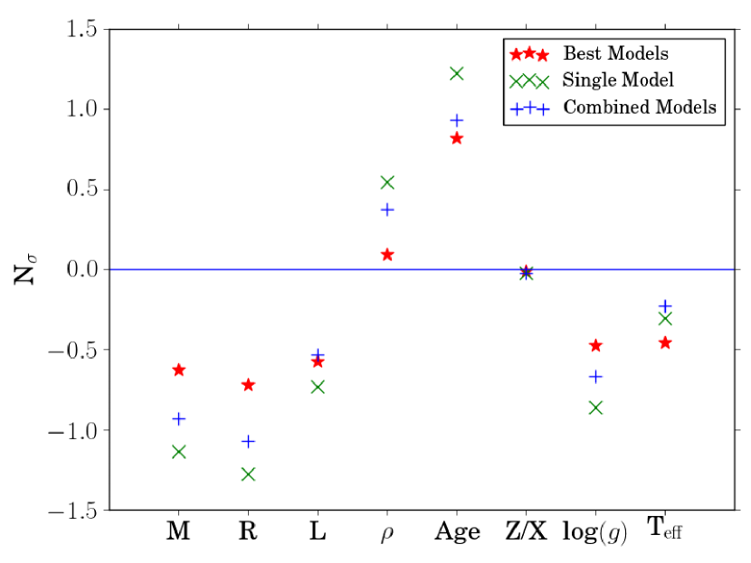
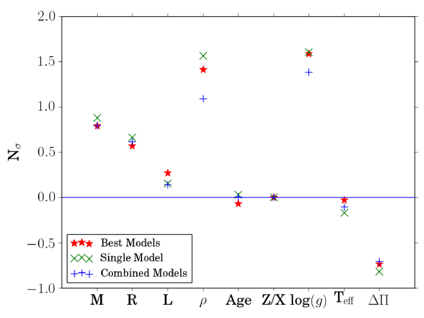
To further examine the quality of the results, the number of standard deviations ($N_{\sigma}$) the output parameter ($x_{\rm{calc}}$) lay from the true value ($x_{\rm{true}}$) was determined using

$$N_{\sigma}=\frac{x_{\rm{calc}}-x_{\rm{true}}}{\sigma}.$$ (2)

These tests are shown in Fig. 8. It is clear that the best MCMC models outperform both combined and single models. The higher performance of the combined run stems from the increased abundance of data, providing a better convergence on the real value than a single run. As the results always lay within $1.5\sigma$ of the result, we can conclude that the fits were successful.

Figure 8: $N_{\sigma}$ steps from the true value of each calculated parameter for the unperturbed (green), combined (blue) and best MCMC (red) models for the MS tests.

5.1.2 Red Giants

Using the same track and set of classical constraint parameters for consistency, a model from the RGB grid was selected and subjected to the same tests as the MS model. Frequency uncertainties were constructed as for the MS observational file. Uncertainties on the classical constraints were again consistent with the literature. The period spacing, $\Delta\Pi$, was included as a grid parameter ($\sigma_{\Delta\Pi}=1\%$, Vrard et al. 2016) and consequently as one of the outputs in the results.

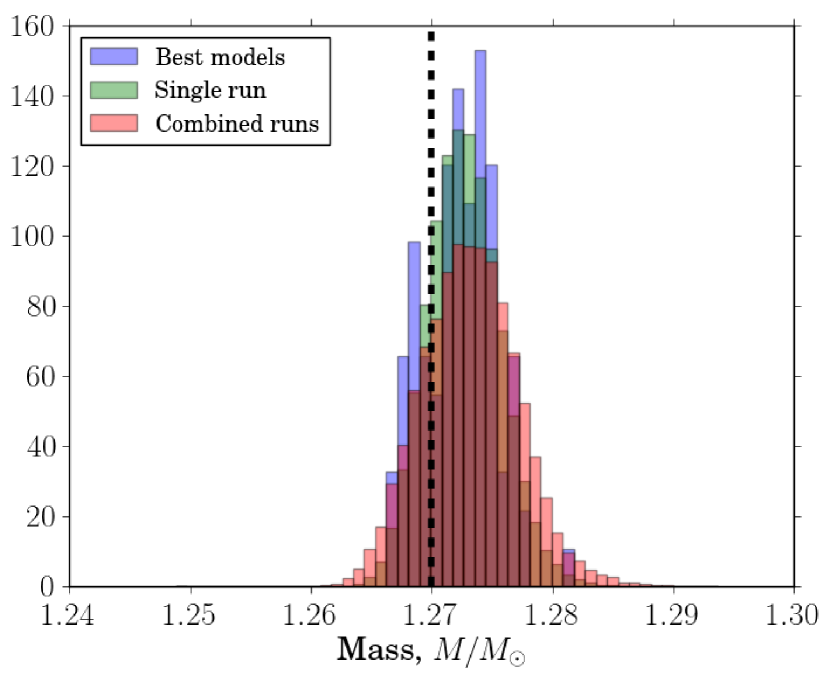
As before, PDFs of the mass and radius, in addition to an $N_{\sigma}$ plot for all parameters, have been included. Figure 9 shows a tight relationship between each of the three model runs, sharing common peak values. The widths of the distributions of the RGB PDFs are broader than their MS counterparts. This is reflected in the increased uncertainties of the output values. Using fewer frequencies compared to the MS runs (9 RGB, 21 MS) and only $l=0$ modes may contribute to this factor, but it is inherent from broader studies that larger RGB compared to MS uncertainties are to be expected. A larger number of models are also rejected when searching the RGB grid, indicating fewer models are likely to be selected around the desired solution.

Figure 9: The mass (left) and radius (right) PDF distributions for RGB the single model (green), 100 realisations (red) and best models from the MCMC runs (blue). The model mass and radii are 1.27 M_⊙ and 4.403 R_⊙, indicated by the vertical black, dotted line.

The trend in Fig. 10 closely resembles that observed in Fig. 8, but little should be read into this. Repeating the trials on multiple MS and RGB models from tracks in different regions of the grid resulted in different $N_{\sigma}$ parameter distributions with each track. Each set of parameters returned is subject to different over/under estimations from models resulting from their grid location and the boundary conditions imposed on them. This variation in model determined variables and their associated likelihoods means consistency between $N_{\sigma}$ patterns should not be expected from model to model. The focus should therefore be on the distribution of $N_{\sigma}$ values which are all satisfactorily $<1.5\sigma$ in each case.

Figure 10: $N_{\sigma}$ steps from the true value of each calculated parameter for the unperturbed (green), combined (blue) and best MCMC (red) models for the RGB tests.

5.2 The Sun

Besides artificial data, we used AIMS to reproduce solar data from the BiSON network of telescopes (Broomhall et al., 2009; Davies et al., 2014; Hale et al., 2016), using the $l=0,1,2$ and $n=18-23$ modes. The frequency uncertainties were increased by a factor of $\sqrt{21/4}$ (Libbrecht, 1992; Toutain & Appourchaux, 1994; Ballot et al., 2008) to perform a Sun-as-a-star analysis. We recall that a solar-calibrated value of the mixing length was used in the grid.

When working with real data, it is necessary to account for surface effects, which are not present in tests performed with artificial data. We used the two-term Ball and Gizon surface correction (Ball & Gizon, 2014), although other corrections are also included in AIMS: Ball and Gizon single-term (Ball & Gizon, 2014); Kjeldsen (Kjeldsen et al., 2008); Sonoi (single-term, scaling, two-term - Sonoi et al. 2015).

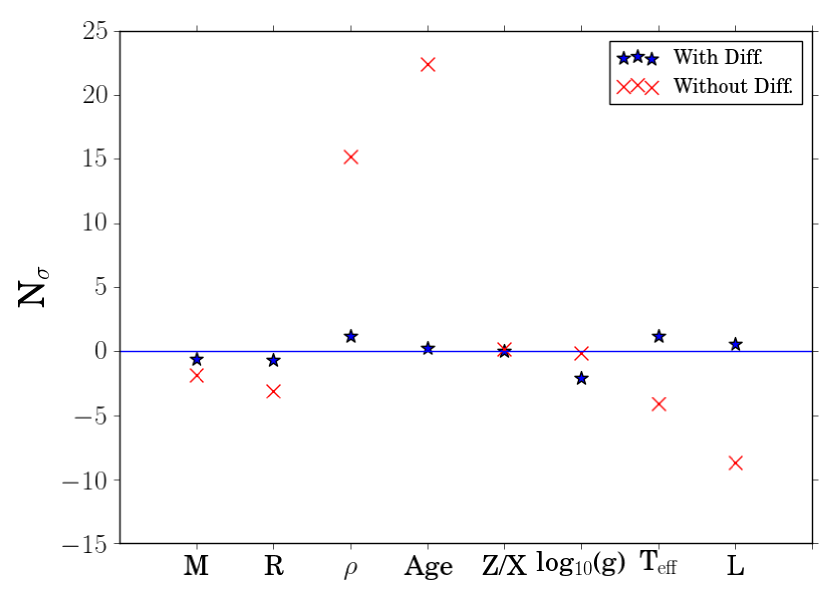
The fits were performed using two grids: the nominal CLÉS MS grid and an identical grid, but with microscopic diffusion included in the modelling (re-calibrated mixing length: 1.81). From Table 2, we can see that models without diffusion can reproduce quite well both the solar mass and radii, although not at the 1$\sigma$ level, but that they present inaccuracies in age of about $\sim$1Gyr. This is in agreement with helioseismic results which reject solar models without microscopic diffusion (Christensen-Dalsgaard et al., 1993). However, models with microscopic diffusion show excellent agreement with solar values (Thoul et al., 1994). Fig. 11 confirms this, displaying $N_{\sigma}$ results for multiple parameters of the Sun for grids with (blue stars) and without (red crosses) microscopic diffusion.

Table 2: Comparison of Solar parameters using grids with and without microscopic diffusion. Mass and radius are given in Solar units, density in g cm^-3 and age in Myrs. Literature density and age are from Reese et al. (2012) and Bahcall et al. (1995).

Parameter	With Diff.	Without Diff.	Literature
Mass	$0.997\pm 0.005$	$0.994\pm 0.003$	1.0
Radius	$0.999\pm 0.002$	$0.996\pm 0.001$	1.0
$<\rho>$	$1.412\pm 0.001$	$1.4183\pm 0.0005$	$1.4104\pm 0.0012$
Age	$4578\pm 31$	$5264\pm 31$	$4570\pm 20$

Figure 11: $N_{\sigma}$ steps from the true value of the mass, radius, density, age (taken to be $4.57\pm 0.02$ Gyr, Bahcall et al. 1995), $Z/X$ ratio, log₁₀(g), $T_{\rm{eff}}$ and luminosity for the Sun for the grids with (blue stars) and without (red crosses) diffusion.

With Diffusion	Without Diffusion

Figure 12: Frequency residuals ($\nu_{\rm{obs}}-\nu_{\rm{theo}}$) comparison between the observed and theoretical frequencies output by AIMS for the grid with (left) and without (right) microscopic diffusion. The residuals subplot for the results with diffusion shows the residuals for frequencies $>3750\mu$Hz. These residuals are much larger and therefore shown in a separate subplot to allow the underlying trend in the residuals to be observed.

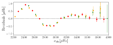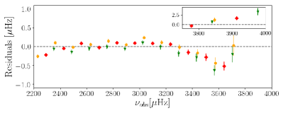
Figure 12 shows the difference between the observed frequencies ($\nu_{\rm{obs}}$) and the theoretical (surface corrected - s.c., $\nu_{\rm{theo\,s.c.}}$) frequencies returned by AIMS for the grids with (left) and without (right) diffusion respectively. All available Solar frequencies are shown. Residuals are shown to illustrate the quality of the interpolation process, hence the robustness of the parameter determinations. A periodic trend is seen in both cases, with a much higher emphasis for the non-diffusive grid. This trend is the result of the large mismatch of helium abundance between the theoretical model and the Sun. Larger disparities are also observed above 3700 $\mu$Hz as a consequence of the surface effects. This clearly illustrates the difficulties and weaknesses of using individual frequencies as direct constraints as the surface effects could bias the modelling results. Using constraints such as frequency ratios for MS stars can help mitigate such effects.

Looking at the reduced $\chi^{2}$ values of the frequencies, it seems sensible to favour the values of the Solar parameters determined using the grid including diffusion:

$$\chi^{2}=\sum_{\rm{i}}\frac{(\nu_{\rm{theo\,s.c.,i}}-\nu_{\rm{obs,i}})^{2}}{\sigma_{\rm{i}}^{2}}$$ (3)

$$\chi_{\rm{red}}^{2}=\frac{\chi^{2}}{d.o.f.}$$ (4)

where $d.o.f.$ (degrees of freedom) is the number of input parameters minus the number of free parameters, and $\sigma$ the compound uncertainty on the frequencies. Indeed, $\chi^{2}_{\rm{red,diff}}=11.4$ whereas $\chi^{2}_{\rm{red,non-diff}}=52.5$. Testing the hypothesis that the model values are true, p values of 0.88 ($\chi^{2}_{\rm{red,diff}}$) and 0.07 ($\chi^{2}_{\rm{red,non-diff}}$) were returned. The order of magnitude difference between the reduced $\chi^{2}$ values clearly indicates that the grid including diffusion is superior for the Solar analysis. As mass, radius and age are all within 1$\sigma$ of the Solar values for this grid, we can conclude that the processes within AIMS perform well enough to produce the results to a high degree of accuracy. All of the uncertainties are lower than one would expect to find in the literature (see Silva Aguirre et al. 2017 for recent Solar values from multiple grids and codes) as they are of the same order of magnitude as in tests using artificial data.

Table 3: Solar parameters and uncertainties determined by AIMS using the frequency separation ratios r_0,1, r_0,2 and r_1,0 as asteroseismic constraints. Mass and radius are given in Solar units, density in g cm^-3 and age in Myr. The diffusive grid was used.

Parameter	r0,1	r1,0	r2,0
Mass	$1.01\pm 0.02$	$1.00\pm 0.02$	$0.99\pm 0.03$
Radius	$1.01\pm 0.03$	$1.00\pm 0.03$	$0.99\pm 0.03$
$\rho$	$1.40\pm 0.10$	$1.42\pm 0.10$	$1.44\pm 0.10$
Age	$4614\pm 258$	$4549\pm 204$	$4603\pm 139$

To determine whether the small uncertainties resulted from the model or the use of individual mode frequencies, the Solar data was also tested using the r_0,1, r_0,2 and r_1,0 frequency separation ratios (Roxburgh & Vorontsov 2003; grid including microscopic diffusion used). An improvement in the returned parameters can be expected, as the ratios focus more on the stellar interior (Roxburgh & Vorontsov, 2003; Otí Floranes et al., 2005). Additionally, their reduced sensitivity to surface effects should also lead to an improvement. This is confirmed by the results in Table 3. The frequency ratios give values consistent with the $\nu_{\rm{ind}}$ results and the expected Solar values, but with larger uncertainties. When using solely the frequency ratios, one filters out additional information (e.g. on the mean density of the star) and thus naturally the uncertainties are increased. While this leads to larger uncertainties on the stellar parameters, this degree of precision can also be seen as more robust with respect to systematic effects which can be underestimated when directly fitting the individual frequencies.

6 Impact of using different combinations of seismic and non-seismic constraints

In addition to testing the main functionalities of AIMS, the effect of the inclusion of certain combinations of constraints within the input observation file were explored. For all tests presented so far, the classical constraints used have been $\nu_{\rm{max}}$, $T_{\rm{eff}}$, $L$ and [Fe/H]. In addition to these constraints, equal weighting has been given to the asteroseismic (input frequencies, $\nu_{i}$) and classical constraints.

6.1 Main Sequence Fits

Four tests were performed on a single main sequence model (the same model used in Sect. 5.1.1) from within the grid, with the effect on the PDF distributions and uncertainties of the mass, radius and age of the artificial star recorded. The constraint variations were as follows:

1. $T_{\rm{eff}},L(\sigma_{Gaia})$, [Fe/H], no acoustic oscillation frequencies

2. $T_{\rm{eff}}$, [Fe/H], acoustic oscillation frequencies, no $L$

3. $T_{\rm{eff}},L(\sigma_{Gaia})$, [Fe/H], r_0,2

4. $T_{\rm{eff}},L(\sigma_{Gaia})$, [Fe/H], acoustic oscillation frequencies

Figure 13: Comparison of input classical and seismic constraints for mass (left), radius (centre) and age (right) determination. The normalised distributions represent the different classical constraint criteria: (i) - green, dot-dashed; (ii) - blue, dashed; (iii) magenta, dotted; (iv) - red, solid.

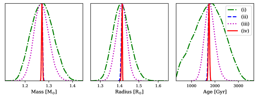
Figure 13 displays the PDFs for mass, radius and age determinations. The inclusion or exclusion of luminosity from the constraints appears to have a minimal impact on the precision between cases (ii) and (iv). The increase in precision on each parameter may not be as significant as the inclusion of asteroseismology (narrowing of distributions observed in both cases), but an improvement is still observed when luminosity is included. Should other parameters (e.g. initial He abundance) be free to vary, an independent constraint on luminosity is important to lift any existing degeneracies present when using only seismology.

Table 4 shows the uncertainties for each set of constraints. Test (i) returns uncertainties of order of the typical literature values for age, mass and radii respectively, but tests (ii) and (iv) return values at least an order of magnitude smaller. The addition of more free parameters to the grid and the intrinsic differences they would cause between models would increase these uncertainties to be closer to those expected. However, the trend between constraint sets is clear. The decision to include or exclude the acoustic oscillation frequencies has a significant impact on all parameters, reducing the percentage errors by an order of magnitude.

Though reduced compared to case (i), case (iii) uncertainties are of the same order of magnitude despite the inclusion of asteroseismology and are in line with the best literature values. This illustrates the difference in precision achievable with the inclusion of global asteroseismic parameters compared to the use of individual mode frequencies when the same classical constraints are available. The potential improvement in precision to be gained underlines the importance of the development of analysis codes, such as AIMS, capable of using individual acoustic oscillation frequencies for the furthering of asteroseismic studies.

Table 4: Percentage uncertainties for the determined values of mass, radius and age for the MS model used in the observational tests, subject to the tested combinations of classical and asteroseismic constraints.

Constraint	Age ($\%$)	Mass ($\%$)	Radius ($\%$)
(i)	34.64	3.69	3.12
(ii)	1.69	0.18	0.22
(iii)	12.65	2.48	1.98
(iv)	1.41	0.16	0.18

6.2 Red Giant Fits

The process was repeated for an RGB model from the grid to illustrate that, despite less convincing interpolation results than on the MS, it also performs well in this regime. Consequently, a more comprehensive approach was taken. We compare the results of AIMS for red giant stars to an extensively used, pre-existing stellar parameter determination code to prove the capability of AIMS as an analysis tool. We chose the PARAM software (da Silva et al., 2006; Rodrigues et al., 2014, 2017), which is quite similar to AIMS in its philosophy, with the only significant difference being that AIMS uses asteroseismic data as an input. We run AIMS without using the input mode frequencies to make a more informed comparison between the capabilities of both codes.

A recent work by Rodrigues et al. (2017) (hereafter R17) investigates the effects of various combinations of constraints on the accuracy of stellar parameter determinations for a series of artificial red giant and red clump stars using PARAM. We repeated these tests using the same sets of classical and global seismic constraints in AIMS and our own RGB model. 10 different combinations of constraints were used:

(i)	$\Delta\nu$			(vi)	$\Delta\nu,\nu_{\rm{max}},\Delta\Pi,L$
(ii)	$\Delta\nu,\nu_{\rm{max}}$			(vii)	$\nu_{\rm{max}},L$
(iii)	$\Delta\nu,\Delta\Pi$			(viii)	$\log_{10}(g),L$
(iv)	$\Delta\nu,\nu_{\rm{max}},\Delta\Pi$			(ix)	$\Delta\nu,\log_{10}(g)$
(v)	$\Delta\nu,\Delta\Pi,L$			(x)	$\Delta\nu,L$

From the above list, it is clear that asteroseismic parameters are still to be used as initial constraints with the large frequency separation ($\Delta\nu,\sigma_{\Delta\nu}=0.05\mu$Hz), frequency of maximum power ($\nu_{\rm{max}},\sigma_{\nu_{\rm{max}}}=2\%$) and period spacing ($\Delta\Pi,\sigma_{\Delta\Pi}=1\%$) featuring heavily. These parameters are all global seismic properties and are not necessarily reliant upon determination of individual frequencies. Hence, they can be input as classical constraints. In addition to the listed constraints, the effective temperature ($\sigma_{T_{\rm{eff}}}=80$ K) and metallicity ($\sigma_{[\rm{Fe/H}]}=0.1$ dex) were included for each case as in R17. The uncertainties used on $L$ and log₁₀(g) were $3\%$ and 0.1 dex respectively. It should be noted that case (iii) of R17 was ignored here, with a value of $\Delta\nu$ calculated from the frequencies used throughout.

Figure 14 displays the results of these tests as the distributions of the determined values normalised to the true parameter values. In addition to the above sets of constraints, the model was tested using the standard constraints used throughout this work and with a direct fit of the individual mode frequencies. This is labelled ‘$\nu_{i}$’.

Figure 14: Comparison of the posterior probability distributions for multiple combinations of constraints used as inputs to AIMS without the use of the individual mode frequencies. The distribution marked ‘AIMS inputs’ shows the result obtained if the individual mode frequencies are used.

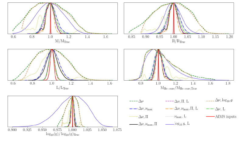
To further analyse the distributions, Table 3 from R17 has been recreated. Table 5 contains the relative uncertainties for the mass and age of the tested model for each combination of constraints. The majority of the results follow typically Gaussian distributions, but cases (i), (viii) and (ix) show asymmetry in their mass distributions. The sampling of the mass in these cases has reached the lower end of the grid, introducing a sampling bias as a build up of low mass samples occurs. This causes the asymmetry observed, which propagates to other parameters.

A direct comparison between the two sets of results is not appropriate due to the different models used, but a comparison of the overall trends is meaningful. The attained values vary, but in general the distributions follow those of R17. This is reassuring and confirms that AIMS reacts to certain combinations of constraints in an expected manner.

Table 5: Fractional uncertainties for each combination of input constraints for AIMS run as PARAM. The RGB results from table 3 of R17 are displayed for direct comparison.

Constraints	$\sigma_{M}/M$		$\sigma_{\rm{Age}}/\rm{Age}$
	AIMS	R17	AIMS	R17
$\nu_{i}$	0.002	-	0.029	-
$\Delta\nu$	0.184	0.173	0.735	0.734
$\Delta\nu,\nu_{\rm{max}}$	0.061	0.078	0.230	0.284
$\Delta\nu,\Delta\Pi$	0.119	0.109	0.475	0.336
$\Delta\nu,\nu_{\rm{max}},\Delta\Pi$	0.047	0.054	0.190	0.192
$\Delta\nu,\Delta\Pi,L$	0.048	0.043	0.131	0.122
$\Delta\nu,\nu_{\rm{max}},\Delta\Pi$, L	0.037	0.034	0.110	0.097
$\nu_{\rm{max}},L$	0.041	0.039	0.108	0.107
$\log_{10}(g),L$	0.138	0.124	0.544	0.427
$\Delta\nu,\log_{10}(g)$	0.166	0.173	0.590	0.727
$\Delta\nu,L$	0.055	0.052	0.146	0.143

Considering previous statements regarding AIMS uncertainties, the fractional uncertainties shown in Table 5 are comparable to those of PARAM. Removing the use of individual mode frequencies causes the inflation of the uncertainties due to the smaller number of constraints. Consistency between codes here is important to show that when global asteroseismic parameters are used as constraints, AIMS performs as well as a pre-established and trusted software. Some variation of the fractional uncertainties compared to R17 is present but likely stems from the differences in model parameters and grid properties, as well as modelling codes used in these tests.

Using all of the available information from the mode frequencies improved the fractional uncertainties with values of 0.002 and 0.029 in mass and age respectively. This test case also produces the best PDFs in Fig. 14, showing the potential of using constraints determined from individual frequencies.

In order to demonstrate the difference in performance between using all the available modes and only the global asteroseismic parameters on an MS star, the model used in section 5.1.1 was re-run using the same constraints and configuration as test (ii). Though it was not possible to perform such a comparison with PARAM results, the consistency of the AIMS results without the use of individual frequencies with PARAM allows meaningful comparisons.

Figure 15 shows the result comparison of two separate runs for mass and radius as before, as well as the relations for the luminosity, surface gravity and evolutionary parameter - age. An offset between the peaks of the distributions is present for various parameters, caused by the known helium-mass degeneracy (see Baudin et al. 2012 and references therein). As tighter constraints are placed on the luminosity of the star when asteroseismology is used, these degeneracies become lifted, allowing for tighter distributions around the expected solutions.

Table 6: Percentage uncertainty of calculated variables with and without the use of individual frequencies as a constraint for an MS artificial model. ‘With $\nu$’ indicates that the individual frequencies were used in the analysis. $<\Delta\nu>$ indicates the runs without the use of the individual frequencies, but inclusion of the average large frequency separation as a constraint. The $l=0,1,2$ modes were used.

Model	$\sigma_{\rm{Mass}}$	$\sigma_{\rm{Radius}}$	$\sigma_{\rm{Lum}}$	$\sigma_{\rm{g}}$	$\sigma_{\rm{Age}}$
MS (with $\nu$)	$0.14\%$	$0.06\%$	$0.48\%$	$0.01\%$	$1.18\%$
MS ($<\Delta\nu>$)	$2.96\%$	$1.12\%$	$2.71\%$	$0.10\%$	$15.48\%$

Figure 15: Comparison of the normalised posterior probability distributions for the MS model both with (red, solid) and without (green, dashed) the use of the individual mode frequencies.

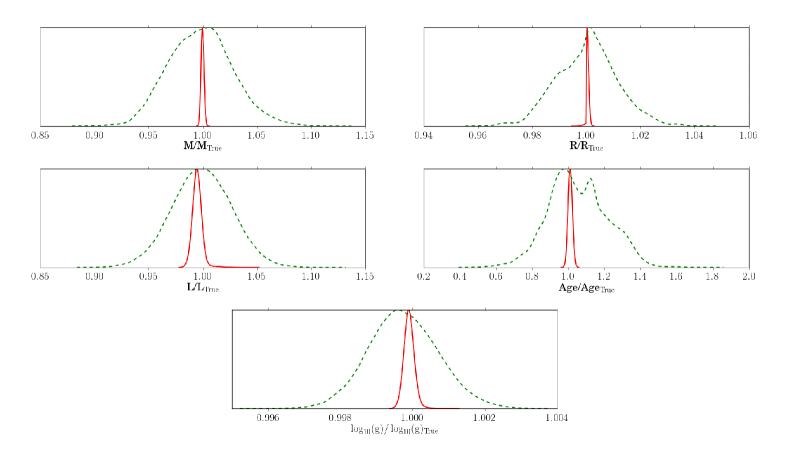
Table 6 shows the statistical trends observed in the related figures, giving the percentage uncertainty on each of the relevant parameters for the cases where the individual frequencies were used and when only global asteroseismic constraints were applied. It should be stressed that the uncertainties displayed in Table 6 are purely statistical and do not account for any systematics within the code. Despite this, the effect of including the individual frequencies in the analysis is clear from Table 6. A reduction in uncertainty is seen for all parameters when using the individual frequencies, displaying the benefits of using this additional information. However, as discussed before, the direct use of individual frequencies as constraints can lead to underestimated uncertainties. This is particularly true for main-sequence stars, which often have very rich oscillation spectra. In that sense, being able to use frequency ratios in AIMS allows us to obtain a more realistic precision on stellar parameters and should generally be preferred.

The reduction between the RGB and MS uncertainties is not of the same order for case (vi) for mass and age (case vi contains the initial artificial RGB test classical constraints and therefore is most appropriate to compare). The uncertainties in mass and age on the RGB decrease by factors of 18 and 4, while on the MS the reduction is by a factor of 20 and 15 respectively. The reduction in mass is quite similar for each evolutionary state, but the reduction in age is an order of magnitude greater for the MS. This is mainly due to the observed frequencies and the additional information they carry on the internal stellar structure. Indeed, the RGB fit used 9 frequencies while 21 frequencies were used on the MS. Besides the number differences, the MS fit used modes of $l=0,1$ and $2$, containing a lot of information on the evolutionary stage on the MS, whereas the RGB fit only used radial modes. The $\ell=1$ and $\ell=2$ modes can of course be included within the RGB grid. However, their highly non-linear behaviour and the decreased sensitivity of the small separations to age in evolved stars (e.g. see Montalban et al. 2010), currently precludes their direct use in AIMS.

To further illustrate the impact of the inclusion of the $\ell=1$ and $\ell=2$ modes, an additional test on the MS using only the $\ell=0$ modes from the previous tests (7 in total) was performed. The reduction in uncertainty in this instance was only a factor of $\sim 5$ in age, much more in line with the RGB results. This demonstrates the reliability with which stellar parameters can be derived and also points towards the potential improvement to make with RGB grids and data sets containing more than just the $\ell=0$ mode frequencies.

7 Discussion and Conclusion

We have presented a new, open source, code for the determination of stellar parameters. It is unique as it is currently the sole code using a Bayesian and MCMC algorithm approach with grid interpolation to carry out asteroseismic inferences. The code’s flexible, multidimensional approach to the analysis allows the user to analyse data as a function of 2 or more fixed grid parameters, affording more control over the analysis dimensions. We executed a comprehensive testing phase and presented the results. All aspects of the program were analysed, with the results proving satisfactory.

A test of the interpolation procedures revealed the accuracy to which the interpolation function within the program returns known values from within the grid. Primarily, the tests focused on the interpolation of the radial mode frequencies of the MS and RGB grids, showing that AIMS provides accurate interpolations well above the threshold values set from the literature. Additional inputs (e.g. mass, age, radius…) were then also tested and again found to be returned at a level matching or exceeding the desired threshold.

The parameter determination tests were very informative. Primary tests with artificial data shed light on some potential limitations of both the analysis code and underlying grid. We showed that the parameter uncertainties determined by AIMS are approximately an order of magnitude smaller than typically reported in the literature. Further investigations confirmed that the statistical analysis and propagation of observational uncertainties were robust. The uncertainties stated by AIMS are thus statistical and do not account for biases in the input physics or model selection.

The artificial data tests were satisfactory, with parameters lying within a few $\sigma$ of the true results. The input parameters of the model were not returned, but the results were sufficiently close to the input values for this not to be of great concern. Data for the Sun were analysed to test AIMS on real data with clearly defined parameters for comparison. As expected, the precision achieved when including individual oscillation modes leads to a comparable accuracy with the known values only if one has flawless models. As shown here, this objective is yet to be achieved. One can use the evidence from comparisons of a diffusive and non-diffusive grid to highlight the limitations of certain models and the need to improve upon model selection. As AIMS is strongly coupled to the input grid, its performance depends on the standard of the grid used and the final model selection and returned parameters are ultimately a reflection of this.

The AIMS code is highly flexible in terms of the parameter constraints one can use in the analysis. The code can be operated using individual mode frequencies, frequency ratios or large frequency separations as asteroseismic constraints. It is also possible to operate the code without these options, simply using classical constraints instead. Full posteriors are returned for determined parameters in each case, meaning any correlations are taken care of in the analysis process. The effect of altering the classical and asteroseismic constraints associated with the input observational file was explored, with the impact of including or excluding any asteroseismic constraints extremely clear. The inclusion of asteroseismic constraints improved the internal precision by a factor 2-20 for both the RGB and MS stars respectively for all of the tested parameters ($M,R,\rho$, age, $Z/X$, log₁₀(g), $T_{\rm{eff}}$, $L$), underlining how important asteroseismology is to AIMS for accurate inferences and the improvement in measurements this technique allows for.

A comparison with an established stellar parameter code, PARAM, gave a valuable insight into the performance of AIMS. For red giant stars, a set of artificial data similar to those used in R17 was analysed using a variety of constraint combinations, including multiple global asteroseismic parameters. Some variation from the expected values for different combinations was observed, but upon comparison with the work in R17, the distributions and relative uncertainties show comparable trends. The similarity in results to an established code brings confidence to those being output by AIMS, showing that it performs to the standard expected by the field, even without the use of the individual mode frequencies it is designed to use.

The primary focus of constraint testing was on the precision to which the code can operate, but pushing it to the challenging limits of using the best constraints - i.e. individual oscillation frequencies with uncertainties of the order of $10^{-2}\mu$Hz. The robustness shown here by the results achieved give confidence to explore more possibilities with the code.

Our tests show that, when using individual mode frequencies as constraints, one is in principle able to infer properties with exceedingly high precision. The latter, however, should not be taken as realistic expectations concerning accuracy. Individual mode frequencies are affected by systematic effects that will dominate the uncertainties on the inferred properties. We do not explore such effects in this work, except from the enlightening case of the Sun, where fitting individual mode frequencies results in very high precision estimates of its global properties, which are, however, highly inaccurate if one uses inaccurate models (see Sec. 5.2). This strong model-dependence is attenuated when one uses frequency ratios, as shown in the literature, at the cost of a reduced precision. Explorations of the systematic uncertainties in the models and the inclusion of additional free parameters (e.g. $Y_{\rm{init}}$, mixing length, surface effects) provide additional challenges to progress the code and maintain a high quality analysis tool for the community, and will be presented in a forthcoming work (e.g. see Nsamba et al. 2018). On a positive note, and as demonstrated by the tests using Solar data, AIMS can be used for the comparison of competing models which can be selected using Bayesian inference, as derived from the full posterior distributions of various estimated properties. These tests will be instrumental to promote the development of next generation stellar models, and will improve our ability to determine stellar ages and chemical yields, with wide impact e.g. on the characterisation and ensemble studies of exoplanets, on evolutionary population synthesis, integrated colours and thus ages of galaxies.

The overall outcome of this work has proven Asteroseismic Inference on a Massive Scale to be a flexible, high precision stellar parameter determination program, fit for use to bring tighter constraints to the determinations of stellar parameters through robust asteroseismic analysis and grid modelling for both dwarf and giant stars. Its flexibility and open-source nature makes AIMS a suitable starting point for the development of the pipelines of future missions such as PLATO (Rauer et al. 2014). Moreover, its output can also be used for additional seismic investigations with for example non-linear inversion techniques as developed by Roxburgh (2002) or linear inversions of structural indicators (Reese et al., 2012; Buldgen et al., 2015, 2018b).

Appendix A

A.1 Track Interpolation

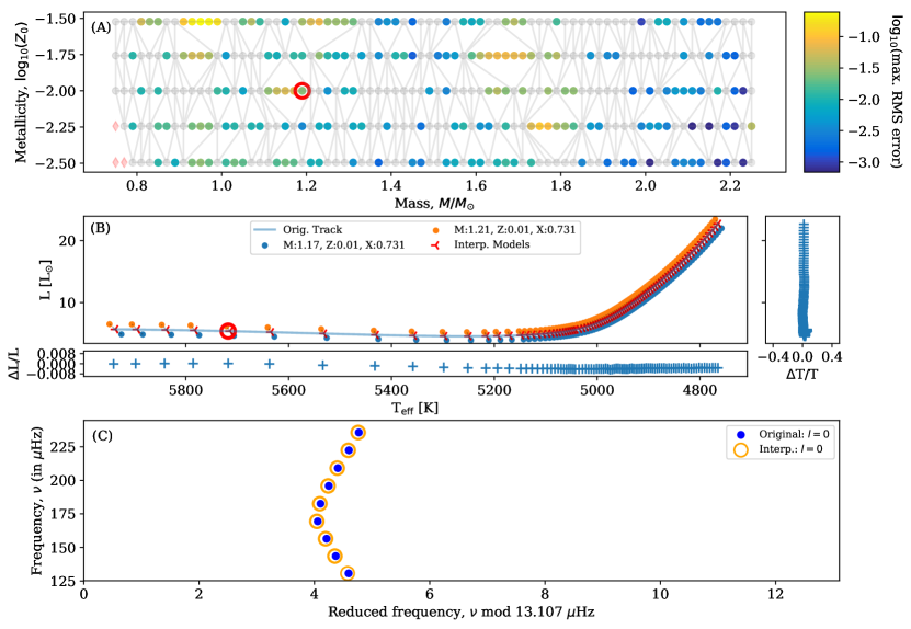
Figure 16 is as Fig. 5, but for a track/model selected from the interpolation tests of the RGB grid. A 1.19 M_⊙, $X_{\rm{init}}$ = 0.731, $Z_{\rm{init}}$ = 0.0100 track is recovered here from models 0.02M_⊙ either side of the original track and of the same $X_{\rm{init}}$ and $Z_{\rm{init}}$ values. The frequency replication is slightly more uncertain than for the MS example (max. log₁₀ error of -2.088), but again excellent parameter residuals and minimal shifts in frequencies show that the process is working well.

Figure 16: Results as for Fig. 5. A 1.19 M_⊙, $X_{\rm{init}}$ = 0.731, $Z_{\rm{init}}$ = 0.0100 track is tested here, but with a model from the RGB grid. A maximum interpolated frequency error of -2.088 is returned for this track and the mass of the Helium core is used as the interpolation parameter. The values of $\Delta$T/T have been increased by a factor of 100 for ease of plotting. The frequencies in (C) have been increased by 5$\mu$Hz to centre the frequency pattern.

A.2 Parameter Interpolation

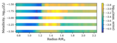
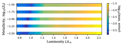
Examples of the interpolation plots for radius and luminosity for the artificial main sequence star analysed in the main text are shown in Fig. 17. The maximum uncertainty for each evolutionary track is shown as per the main text.

Figure 17: Left: Magnitude of the radius errors for the MS grid. Right: Magnitude of the luminosity errors for the MS grid. Interpolation from grid points a single increment from the original solution. The black circles show the grid node points. Uncertainties in Solar units.

References

- Adelberger et al. (2011) Adelberger E. G., et al., 2011, Reviews of Modern Physics, 83, 195
- Andersen et al. (2014) Andersen M. F., et al., 2014, in Revista Mexicana de Astronomia y Astrofisica Conference Series. pp 83–86
- Baglin et al. (2006) Baglin A., Auvergne M., Barge P., Deleuil M., Catala C., Michel E., Weiss W., COROT Team 2006, in Fridlund M., Baglin A., Lochard J., Conroy L., eds, ESA Special Publication Vol. 1306, The CoRoT Mission Pre-Launch Status - Stellar Seismology and Planet Finding. p. 33
- Bahcall et al. (1995) Bahcall J. N., Pinsonneault M. H., Wasserburg G. J., 1995, Reviews of Modern Physics, 67, 781
- Ball & Gizon (2014) Ball W. H., Gizon L., 2014, A&A, 568, A123
- Ballot et al. (2008) Ballot J., Appourchaux T., Toutain T., Guittet M., 2008, A&A, 486, 867
- Barber et al. (1996) Barber C. B., Dobkin D. P., Dobkin D. P., Huhdanpaa H., 1996, ACM Trans. Math. Softw., 22, 469
- Baudin et al. (2012) Baudin F., et al., 2012, A&A, 538, A73
- Bazot et al. (2008) Bazot M., Bourguignon S., Christensen-Dalsgaard J., 2008, Mem. Soc. Astron. Italiana, 79, 660
- Borucki et al. (2010) Borucki W. J., et al., 2010, Science, 327, 977
- Broomhall et al. (2009) Broomhall A.-M., Chaplin W. J., Davies G. R., Elsworth Y., Fletcher S. T., Hale S. J., Miller B., New R., 2009, MNRAS, 396, L100
- Buldgen et al. (2015) Buldgen G., Reese D. R., Dupret M. A., 2015, A&A, 583, A62
- Buldgen et al. (2018a) Buldgen G., et al., 2018a, MNRAS,
- Buldgen et al. (2018b) Buldgen G., Reese D. R., Dupret M. A., 2018b, A&A, 609, A95
- Casagrande & VandenBerg (2014) Casagrande L., VandenBerg D. A., 2014, MNRAS, 444, 392
- Casagrande & VandenBerg (2018) Casagrande L., VandenBerg D. A., 2018, MNRAS, 475, 5023
- Christensen-Dalsgaard et al. (1993) Christensen-Dalsgaard J., Proffitt C. R., Thompson M. J., 1993, ApJ, 403, L75
- CoRot Team (2016) CoRot Team 2016, Foreword, doi:10.1051/978-2-7598-1876-1.c001.
- Davies et al. (2014) Davies G. R., Broomhall A. M., Chaplin W. J., Elsworth Y., Hale S. J., 2014, MNRAS, 439, 2025
- Davies et al. (2015) Davies G. R., et al., 2015, MNRAS, 446, 2959
- Davies et al. (2016) Davies G. R., et al., 2016, MNRAS, 456, 2183
- Field (1991) Field D. A., 1991, Advances in Engineering Software and Workstations, 13, 263
- Foreman-Mackey et al. (2013) Foreman-Mackey D., Hogg D. W., Lang D., Goodman J., 2013, PASP, 125, 306
- Gabriel et al. (2014) Gabriel M., Noels A., Montalbán J., Miglio A., 2014, A&A, 569, A63
- Gaia Collaboration et al. (2018) Gaia Collaboration et al., 2018, A&A, 616, A1
- Goodman & Weare (2010) Goodman J., Weare J., 2010, Communications in Applied Mathematics and Computational Science, 5, 65
- Gough (1990) Gough D. O., 1990, in Osaki Y., Shibahashi H., eds, Lecture Notes in Physics, Berlin Springer Verlag Vol. 367, Progress of Seismology of the Sun and Stars. p. 283, doi:10.1007/3-540-53091-6
- Grevesse & Noels (1993) Grevesse N., Noels A., 1993, in Prantzos N., Vangioni-Flam E., Casse M., eds, Origin and Evolution of the Elements. pp 15–25
- Gruberbauer et al. (2012) Gruberbauer M., Guenther D. B., Kallinger T., 2012, ApJ, 749, 109
- Grundahl et al. (2017) Grundahl F., et al., 2017, ApJ, 836, 142
- Guenther & Brown (2004) Guenther D. B., Brown K. I. T., 2004, ApJ, 600, 419
- Hale et al. (2016) Hale S. J., Howe R., Chaplin W. J., Davies G. R., Elsworth Y. P., 2016, Sol. Phys., 291, 1
- Hekker & Christensen-Dalsgaard (2017) Hekker S., Christensen-Dalsgaard J., 2017, A&ARv, 25, 1
- Howell et al. (2014) Howell S. B., et al., 2014, PASP, 126, 398
- Huber et al. (2013) Huber D., et al., 2013, Science, 342, 331
- Iglesias & Rogers (1996) Iglesias C. A., Rogers F. J., 1996, ApJ, 464, 943
- Irwin (2012) Irwin A. W., 2012, FreeEOS: Equation of State for stellar interiors calculations, Astrophysics Source Code Library (ascl:1211.002)
- Kjeldsen & Bedding (1995) Kjeldsen H., Bedding T. R., 1995, A&A, 293, 87
- Kjeldsen et al. (2008) Kjeldsen H., Bedding T. R., Christensen-Dalsgaard J., 2008, ApJ, 683, L175
- Lebreton & Goupil (2014) Lebreton Y., Goupil M. J., 2014, A&A, 569, A21
- Li et al. (2018) Li T., Bedding T. R., Huber D., Ball W. H., Stello D., Murphy S. J., Bland-Hawthorn J., 2018, MNRAS, 475, 981
- Libbrecht (1992) Libbrecht K. G., 1992, ApJ, 387, 712
- Lillo-Box et al. (2014) Lillo-Box J., et al., 2014, A&A, 562, A109
- Lund & Reese (2018) Lund M. N., Reese D. R., 2018, Asteroseismology and Exoplanets: Listening to the Stars and Searching for New Worlds, 49, 149
- Lund et al. (2017) Lund M. N., et al., 2017, ApJ, 835, 172
- Metcalfe et al. (2009) Metcalfe T. S., Creevey O. L., Christensen-Dalsgaard J., 2009, ApJ, 699, 373
- Miglio & Montalbán (2005) Miglio A., Montalbán J., 2005, A&A, 441, 615
- Miglio et al. (2010) Miglio A., et al., 2010, A&A, 520, L6
- Montalban et al. (2010) Montalban J., Miglio A., Noels A., Scuflaire R., Ventura P., 2010, Astronomische Nachrichten, 331, 1010
- Mosser et al. (2012) Mosser B., et al., 2012, A&A, 537, A30
- Nsamba et al. (2018) Nsamba B., Campante T. L., Monteiro M. J. P. F. G., Cunha M. S., Rendle B. M., Reese D. R., Verma K., 2018, MNRAS, 477, 5052
- Otí Floranes et al. (2005) Otí Floranes H., Christensen-Dalsgaard J., Thompson M. J., 2005, MNRAS, 356, 671
- Pérez Hernández et al. (2016) Pérez Hernández F., García R. A., Corsaro E., Triana S. A., De Ridder J., 2016, A&A, 591, A99
- Rauer et al. (2014) Rauer H., et al., 2014, Experimental Astronomy, 38, 249
- Reese (2016) Reese D. R., 2016, AIMS: Asteroseismic Inference on a Massive Scale, Astrophysics Source Code Library (ascl:1611.014)
- Reese et al. (2012) Reese D. R., Marques J. P., Goupil M. J., Thompson M. J., Deheuvels S., 2012, A&A, 539, A63
- Reese et al. (2016) Reese D. R., et al., 2016, A&A, 592, A14
- Ricker et al. (2015) Ricker G. R., et al., 2015, Journal of Astronomical Telescopes, Instruments, and Systems, 1, 014003
- Rodrigues et al. (2014) Rodrigues T. S., et al., 2014, MNRAS, 445, 2758
- Rodrigues et al. (2017) Rodrigues T. S., et al., 2017, MNRAS, 467, 1433
- Roxburgh (2002) Roxburgh I. W., 2002, in Battrick B., Favata F., Roxburgh I. W., Galadi D., eds, ESA Special Publication Vol. 485, Stellar Structure and Habitable Planet Finding. pp 75–85
- Roxburgh & Vorontsov (2003) Roxburgh I. W., Vorontsov S. V., 2003, A&A, 411, 215
- Scuflaire et al. (2008a) Scuflaire R., Théado S., Montalbán J., Miglio A., Bourge P.-O., Godart M., Thoul A., Noels A., 2008a, Ap&SS, 316, 83
- Scuflaire et al. (2008b) Scuflaire R., Montalbán J., Théado S., Bourge P.-O., Miglio A., Godart M., Thoul A., Noels A., 2008b, Ap&SS, 316, 149
- Serenelli et al. (2017) Serenelli A., et al., 2017, ApJS, 233, 23
- Silva Aguirre et al. (2015) Silva Aguirre V., et al., 2015, MNRAS, 452, 2127
- Silva Aguirre et al. (2017) Silva Aguirre V., et al., 2017, ApJ, 835, 173
- Sonoi et al. (2015) Sonoi T., Samadi R., Belkacem K., Ludwig H.-G., Caffau E., Mosser B., 2015, A&A, 583, A112
- Thoul et al. (1994) Thoul A. A., Bahcall J. N., Loeb A., 1994, ApJ, 421, 828
- Torres (2010) Torres G., 2010, ApJ, 140, 1158
- Toutain & Appourchaux (1994) Toutain T., Appourchaux T., 1994, A&A, 289, 649
- Verma et al. (2017) Verma K., Raodeo K., Antia H. M., Mazumdar A., Basu S., Lund M. N., Silva Aguirre V., 2017, ApJ, 837, 47
- Vorontsov (1988) Vorontsov S. V., 1988, in Christensen-Dalsgaard J., Frandsen S., eds, IAU Symposium Vol. 123, Advances in Helio- and Asteroseismology. p. 151
- Vrard et al. (2016) Vrard M., Mosser B., Samadi R., 2016, A&A, 588, A87
- da Silva et al. (2006) da Silva L., et al., 2006, A&A, 458, 609