Comparing Non-Redundant Masking and Filled-Aperture Kernel Phase for Exoplanet Detection and Characterization

Abstract

The limitations of adaptive optics and coronagraph performance make exoplanet detection close to $\lambda/D$ extremely difficult with conventional imaging methods. The technique of non-redundant masking (NRM), which turns a filled aperture into an interferometric array, has pushed the planet detection parameter space to within $\lambda/D$. For high Strehl, the related filled-aperture kernel phase technique can achieve resolution comparable to NRM, without the associated dramatic decrease in throughput. We present non-redundant masking and kernel phase contrast curves generated for ground- and space-based instruments. We use both real and simulated observations to assess the performance of each technique, and discuss their capabilities for different exoplanet science goals such as broadband detection and spectral characterization.

*Steph Sallum, ssallum@ucsc.edu

1 INTRODUCTION

Direct imaging has recently emerged as a viable planet detection and characterization method. Near- to mid-infrared observations are particularly useful for discovering giant planets, since they have relatively low contrast at these wavelengths[1]. Several molecules that are expected to be in giant planet atmospheres have significant opacity in this wavelength range[2], making infrared spectroscopy useful for constraining atmospheric composition. Furthermore, infrared imaging of young planets can constrain evolutionary scenarios such as hot- versus cold-start models, and can distinguish between planetary atmosphere and circumplanetary accretion disk emission.[2, 3, 4]

Typical direct imaging planet searches are limited to angular separations of a few $\lambda/D$. Point-spread function (PSF) deconvolution algorithms are less effective within these separations due to the small number of resolution elements available.[5] Phase leakage in even the highest performance coronagraphic observations prevents high contrast detections within $\sim 1-2~{}\lambda/D$.[6] These limitations make semi-major axes less than $\sim 10$ AU accessible for only the most nearby stars.[7] Expanding this detection parameter space to smaller semi-major axes and/or to more distant stars (including nearby star forming regions[8]) requires novel imaging techniques such as interferometry.

1.1 Non-Redundant Masking

Non-redundant masking[9] is well suited for detecting young, giant planets around more distant stars than those targeted by typical direct imaging surveys. NRM uses a pupil-plane mask to turn a conventional telescope into an interferometric array. The images are the interference fringes formed by the mask, which we Fourier transform to calculate complex visibilities. Since the mask is non-redundant, no two baselines have the same orientation and separation; information from each baseline is encoded in a unique location in Fourier space.

Non-redundancy means that the instrumental component of each Fourier phase can be written as a linear combination of two pupil phases. Calculating closure phases,[10] sums of phases around baselines forming a triangle, eliminates these instrumental phases to first order, leaving behind sums of phases intrinsic to the target. Closure phases are particularly powerful for close-in companion detection because they are sensitive to asymmetries. Since closure phases are correlated, we project them into linearly-independent combinations called kernel phases[12, 11, 13]. We also calculate squared visibilities, the powers on each mask baseline.

Despite the low throughput ($\sim 10\%$), NRM’s superior PSF characterization probes angular separations at and even within the diffraction limit. It has led to detections of both stellar[14] and substellar companions[15, 16], as well as circumstellar disks[17, 13, 18] at these small angular separations. This angular resolution means that spatial scales of $\sim 10$ AU can be resolved for stars $\sim 150$ pc away. NRM led to the discovery of a promising system for planet formation studies, the protoplanetary candidates in LkCa 15.[14] Dual-aperture LBTI masking observations recently resolved a solar-system sized disk around the star MWC 349A[18], at a distance of $\gtrsim 1.2$ kpc from Earth. With a maximum baseline of 23 meters, this is a preview of NRM’s potential on 30-meter class telescopes. Non-redundant masking on current telescopes and on future facilities will expand the exoplanet detection parameter space.

1.2 Filled-Aperture Kernel Phase

Extreme adaptive optics systems have made filled-aperture kernel phase[12] an interesting alternative to non-redundant masking. Kernel phase involves treating a conventional telescope as if it were a redundant array. Redundancy prevents Fourier phases from being written as a linear combination of pupil-plane phases in general. However, in the high Strehl regime (where instrumental pupil plane phases are small), one can justify Taylor expanding the instrumental wavefront. This means that the redundant instrumental Fourier phases can be approximated as a linear operator on the pupil plane phases. Finding the nullspace of this linear operator yields kernel phases, linearly independent combinations of Fourier phases that are robust to instrumental phase errors to first order. Like closure (and kernel phase) in non-redundant masking, filled-aperture kernel phases are sensitive to asymmetries and are thus powerful for close-in companion detection.

Kernel phase has been demonstrated on archival Hubble Space Telescope observations of ultracool dwarfs[19]. In addition to confirming several known companions to these L dwarfs, it led to the detection of five new binary systems at angular separations of $\sim 40-80$ mas at $\sim 1.1-1.7~{}\mu$m. It has also been applied to ground-based data from Keck[20] and Palomar[21], where it led to the detection of stellar and substellar companions at ($\sim 1-2~{}\lambda/D$). The Keck observations were taken at $\mathrm{M_{s}}$ band, where the high sky background reduces the SNR of masking observations. These kernel phase datasets provided comparable resolution to that expected for NRM, with a shorter integration time.

1.3 Outline of this Paper

Here we compare non-redundant masking and filled-aperture kernel phase in a controlled way, with a specific focus on exoplanet science. We generate simulated datasets for three imagers: NIRC2 on Keck, and NIRCam and NIRISS on James Webb Space Telescope (JWST). We also generate observations for two integral field spectrographs (IFSs): OSIRIS on Keck, and NIRSpec on JWST. Integral field spectroscopy is a particularly interesting kernel phase application, since dispersing the light and applying a pupil plane mask would require long integration times for high signal to noise. Furthermore, when broadband kernel phase observations of bright stars may be unfeasible due to detector saturation, IFS kernel phase observations may not saturate.

We describe the simulated datasets in Section 2. We use the simulated observations to generate contrast curves for both filled-aperture kernel phase and NRM, and to place detection limits on planetary atmosphere and circumplanetary accretion disk models. We present these results in Section 3. In Sections 4 and 5 we discuss the potential of each technique as a method for exoplanet detection and characterization.

2 SIMULATED OBSERVATIONS

Here we simulate non-redundant masking and filled-aperture kernel phase observations for three imagers - Keck NIRC2, JWST NIRCam, and JWST NIRISS - and kernel phase observations for two integral field spectrographs - Keck OSIRIS, and JWST NIRSpec. For the IFS simulations, we use the central wavelength bin to estimate the average performance for each instrument and mode. For all instruments, we compare the two techniques by setting the total amount of observing time, including overheads, to be the same. To ensure a systematic comparison, we use simulated observations so that we can control the various noise sources. When possible, we anchor these simulations using real datasets. We include random noise sources from the star, sky background, and detector. We also simulate changing optical path difference maps for each instrument to account for quasi-static (“speckle”) noise that can lead to kernel phase calibration errors. To simulate these calibration errors, we divide the total observing time for all instruments into observations of a science target and of a PSF calibrator with the same brightness as the science target, but with different quasi-static errors. We break the observations up into “visits.” each of which is a single datacube containing a number of frames on a single target (science or PSF calibrator).

We calculate kernel phases using an updated version of the data reduction pipeline presented in Sallum et al. (2017)[22]. For both Keck and JWST filled-aperture observations, we assume one sub-aperture per mirror segment. This is an arbitrary choice, and while it prevents phase noise due to jumps between mirror segments, denser pupil plane sampling may lead to improved results. We use the “Martinache” kernel phase projection[12], which makes orthonormal combinations of Fourier phases (see Appendix A). We note that other phase combinations can provide higher contrast away from the PSF core; one example is the “Ireland” projection[11], which makes statistically independent combinations of Fourier phases using the kernel phase covariance matrix. This has been shown to boost contrast away from the PSF core in the photon noise limit[11]. Since some of our simulated observations are in the calibration error limit, where the advantages of the “Ireland” projection do not apply[11], we use the “Martinache” projection. The contrast curves shown in Section 3 could be improved by using different projections for probing different angular separations or for different noise regimes.

For both techniques, we apply a super-Gaussian window to create inter-pixel correlations in the Fourier plane before calculating kernel phases. These inter-pixel correlations are helpful for reducing the random kernel phase scatter induced by noise sources such as sky background and detector noise. For NRM datasets we tune the super-Gaussian so that it has a value of 0.9 at the null in the PSF of an individual hole ($\lambda/d_{h}$). For filled-aperture kernel phase the super-Gaussian has a value of 0.9 at $3~{}\lambda/D$. To minimize the impact of sky background and detector noise beyond these regions - where the PSFs have low signal - we use an 8th order super-Gaussian. We note that alternative techniques such as the “Monnier” method[23], and image-plane fringe fitting[24] can reduce random phase scatter without windowing; these have been demonstrated for NRM observations and similar techniques could be applied to filled-aperture kernel phase.

For all instruments and bandpasses, we simulate a grid of stellar apparent magnitudes between $\sim 6$ and 13. This corresponds to absolute magnitudes between $\sim 0$ and 7, at the distance of Taurus ($\sim 140$ pc[8]). While this does not cover the bright end of expected young stars’ absolute magnitudes[25], for filled-aperture kernel phase observations, the apparent magnitude 6 stars are close to or beyond the saturation limit for NIRC2 and NIRCam. We thus focus on this range of stellar brightnesses to compare the two techniques on these instruments. We generate contrast curves for each simulated dataset by comparing the $\chi^{2}$ of the null model ($\chi^{2}_{null}$; a single point source) to a grid of single companion models with different separations, contrasts, and position angles. For each single companion separation, we calculate the average $\chi^{2}$ value for all sampled position angles ($\chi^{2}_{sep}$), and take the 5$\sigma$ contrast to be the contrast at which $\chi^{2}_{sep}-\chi^{2}_{null}=25$. The details of the individual simulations can be found in the following subsections and in Appendix B.

2.1 Keck NIRC2

We simulate kernel phases for filled-aperture and masked Keck NIRC2 observations at Ks = 2.15 $\mu$m, L^′ = 3.78 $\mu$m, and Ms = 4.67 $\mu$m. The filled-aperture and NRM modes yield 45 and 28 kernel phases, respectively. For each target observation, we simulate a cube of $n_{frames}$ frames, each of which is the sum of $n_{coadd}$ coadds (see Tables LABEL:tab:ksnrmobs - LABEL:tab:mskpobs). We add sky background, dark current, and readout noise to the images according to the number of coadds and exposure times; Table 1 lists the relevant noise parameters and other detector information for each bandpass. For all observations, we background subtract each frame and apply any window functions. We then calculate complex quantities for each kernel phase that are analogous to bispectra for closure phases (see Appendix A). Like averaging bispectra for calculating mean closure phases, we average these complex quantities over the cube of images before taking the phase as the mean kernel phase for a single visit.

We simulate optical path difference maps to account for quasi-static PSF aberrations. Keck AO is known to be affected by low-order residual wavefront errors; modeling these as segment piston errors has been shown to produce realistic point spread functions [26]. To simulate point spread functions, we create optical path difference (OPD) maps that are a combination of low- and high-order residual wavefront errors. We generate low-order errors over the entire Keck pupil and on each individual mirror segment. For the entire pupil, we make combinations of the first 20 Zernike modes ($Z_{n}$; excluding tip and tilt), drawing each coefficient from a uniform distribution with a width ($2~{}f(n)$) that depends on the Zernike order (n):

$$OPD_{low}=\sum_{n=0}^{20}\mathrm{Unif}\left(-f(n),f(n)\right)Z_{n}=\sum_{n=0}^{20}C_{low}Z_{n}.$$ (1)

The function $f(n)$ has the form $n^{\alpha}$, and we tune $\alpha$ to match real observations (see below). For the individual mirror segments, we add tip, tilt, and piston errors, drawing each coefficient from a uniform distribution with a fixed width:

$$OPD_{seg}=\sum_{n=0}^{2}\mathrm{Unif}\left(-g,g\right)Z_{n}=\sum_{n=0}^{2}C_{seg}Z_{n}.$$ (2)

Table 1: NIRC2 Noise and Detector Parameters

Band	$\lambda_{c}$	$\lambda/D$	S	ZP	DC	RN	WD	g
	($\mu$m)	(pix)	(mag/arcsec2)	(mag)	(e- / pix / s)	(e- / pix)	(DN)	(e-/DN)
Ks	2.146	4.45	12.66	24.84	0.1	15	18,000	4
L′	3.776	7.83	3.01	23.6	0.1	15	18,000	4
Ms	4.670	9.69	0.23	21.42	0.1	15	18,000	4

Table 2: NIRC2 OPD Parameters

Low-order RMS	160 nm
Low-order order dependence ($\alpha$)	0.2
Low-order evolution parameter ($h$)	0.3
Segment RMS	280 nm
Segment evolution parameter ($h$)	0.3

When we apply this prescription, we use arbitrary normalizations for $f(n)$ and $g$, and then re-scale the final OPD maps to have an RMS tuned to match real observations. We also tune the dependence of the low order Zernike coefficients on Zernike order ($\alpha$). The best OPD parameters are listed in Table 2. These lead to uncalibrated kernel phase scatters of $\sim 1.2^{\circ}$ for L^′ NRM observations (compared to $\sim 1.0-1.5^{\circ}$ for real observations), and Strehl values of 0.55, 0.85, and 0.9 at Ks, L^′, and Ms (consistent with typical Strehls observed using NIRC2), respectively. They also match observed PSF radial profiles to within $\sim 4\%$ fractional error. Figures 1 and 2 show example images and power spectra, respectively, for NRM and kernel phase for each bandpass.

Figure 1: Simulated individual K_s (left), L^′ (center), and M_s (right) images for the observing parameters listed in Table 1. The top row shows filled-aperture data, and the bottom row non-redundant masking data. The images are displayed on a square root scale to highlight structure in the wings of the point spread function. The fields of view are different for the two techniques: the kernel phase images are 45 mas on a side, and the NRM images are 100 mas on a side.

Figure 2: Simulated K_s (left), L^′ (center), and M_s (right) power spectra for a single frame using the observing parameters listed in Table 1. The top row shows filled-aperture kernel phase data, and the bottom row non-redundant masking data. Random noise from the large sky background is apparent in the L^′ and M_s power spectra; building signal to noise in the long baselines requires combining more frames. The scattered points show the sampling locations for calculating kernel phases; they are shown in two colors since the Fourier transform is symmetric.

Figure 3: Example OPD evolution for NIRC2 filled-aperture kernel phase (top) and non-redundant masking (bottom). The left shows an initial OPD made up of both low- and high-order wavefront errors, and the center panel shows the result of evolving the OPD map. The right side shows the difference between the two; it has an rms OPD of 60 nm.

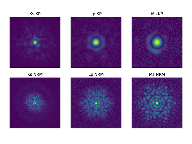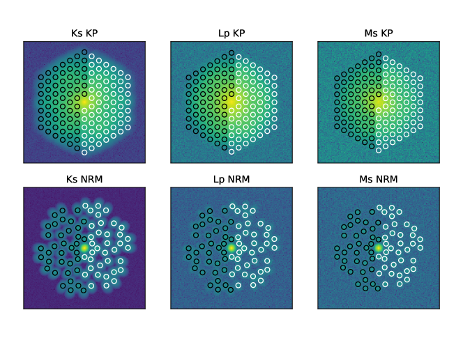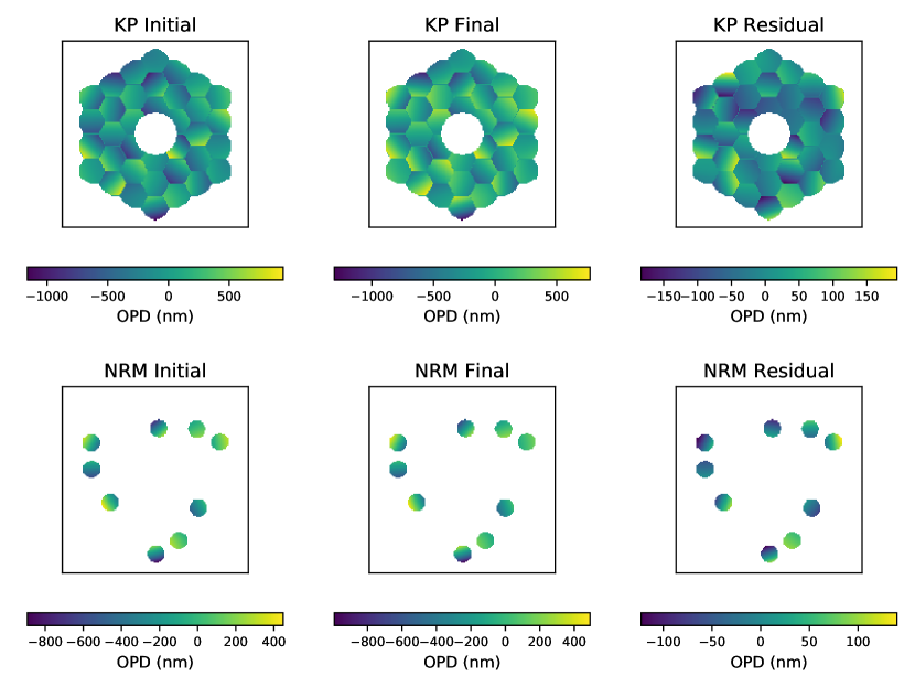Keck’s low-order errors are quasi-static [27] and contribute to calibration errors in the final kernel phases. We thus generate calibrator observations after evolving the low-order and segment OPD Zernike coefficients by a factor drawn from a one-mean uniform distribution with width $2h$. Equations 3 and 4 describe this procedure:

$$C_{n,low,cal}=\mathrm{Unif}\left(1-h,1+h\right)C_{n,low,targ}$$ (3)

$$C_{n,seg,cal}=\mathrm{Unif}\left(1-h,1+h\right)C_{n,seg,targ}.$$ (4)

We use the original and evolved optical path difference maps to generate point spread functions for each target and calibrator observation, respectively. To calibrate, we subtract the simulated calibrator kernel phases from the target kernel phases. We tune the evolution parameter ($h$) so that the calibration decreases the kernel phase scatter by the same amount as it does in typical NIRC2 NRM observations ($h=0.3$). This results in calibrated NRM kernel phase scatters of $\sim 0.2-0.3^{\circ}$ for observations of a L^′ = 5.8 star, consistent with the observed scatter in PSF calibrator observations from Keck at L^′. Figure 3 shows an example of OPD evolution for both techniques; the residual OPD map has $\sim$60 nm rms. We note that this prescription does not include residual AO errors such as fitting error, bandwidth error, or aliasing, which would change on timescales comparable to the AO frame rate (much shorter than the integrations presented here). Adding these effects would make the OPD simulations more realistic, but since they would average over many AO loops and since the simplified prescription can match real observations, we do not include them.

We design a half night of observations for each target star magnitude and bandpass, accounting for overheads. We split the half night into a number of visits to target and PSF calibrator stars. The length of each visit depends on the number of photons collected from the star and sky; for a small number of source photons, kernel phase errors may be dominated by random noise. As the number of source photons increases, the random kernel phase scatter decreases, and the visit approaches the contrast limit - where quasi-static errors dominate over random errors. Longer integrations in this limit do not decrease the kernel phase scatter significantly. Thus we design our visits to be either long enough to reach the contrast limit, or to take 3 hours (half the observing time), since the observing is split evenly between target and PSF calibrator observations. Datasets on brighter stars will contain more visits than datasets on fainter stars. When multiple visits can fit into a half night, we treat them as snapshots at different parallactic angles that change in $5^{\circ}$ increments and have independent calibration errors.

To account for NIRC2 overheads, we treat each visit as a collection of frames and each frame as the sum of a number of coadds. We design each coadd to be long enough to reach 5000 - 10,000 maximum counts - this is to minimize overheads but remain in a linear regime on the detector. We assume a 512 by 512 pixel subframe, which results in a single coadd overhead of 0.05 seconds. We enforce a minimum frame time of 20 seconds, which adds an additional overhead of 2.18 seconds every 20 seconds. We assume that the observations are dithered every 200 seconds to enable sky subtraction, which adds an overhead of 6 seconds for each dither. Lastly, we assume target acquisition overheads of $\sim 90$ seconds per pointing[28]. Tables LABEL:tab:ksnrmobs - LABEL:tab:mskpobs in Appendix B provide frame, coadd, and dither details for each target star brightness. Figures C.1 and C.2 show histograms of the raw (uncalibrated) and calibrated kernel phases for each technique and bandpass for two different target star brightnesses.

2.2 JWST NIRCam and NIRISS

We use the Pandeia engine [29] and WebbPSF software [30] to simulate NIRCam kernel phase and NIRISS aperture masking (AMI) observations to compare the two techniques. NIRCam imaging and NIRISS AMI yield 21 and 15 kernel phases, respectively. Since exoplanets are relatively bright in the near- to mid-infrared, we simulate data for filters centered on wavelengths $\gtrsim 4~{}\mu$m that can be used with NIRISS AMI and NIRCam imaging (F430M and F480M). Since slew and telescope roll overheads are large for JWST, we do not allow the number of visits for the different target stars to vary like we do for NIRC2. We rather assume the observations are made up of two pairs of target - PSF calibrator visits taken at different telescope roll angles 45^∘ apart. We assume that the length of each visit is 1.5 hours, for a total observation time of 6 hours, excluding slew and roll angle overheads. When designing the observations, we account for detector overheads within each 1.5 hour visit.

JWST visits are split into sets of integrations, each of which is composed of a number of groups. To calculate overheads, for each target magnitude we first find the maximum number of groups ($n_{g}$) that can be used in a single integration without saturation. For NIRCam imaging, this means choosing the readout mode that provides the maximum integration time, but for NIRISS AMI only one readout mode is available. We then assume that each visit is composed of the maximum number of $n_{g}$-group integrations ($n_{i}$) that can be acquired in 1.5 hours, given that each integration comes with a readout overhead (0.0494 seconds for NIRCam in a sub64P subarray, and 0.0745 seconds for NIRISS in a sub80 subarray). When the remaining time after $n_{i}$ integrations allows for more than a single group, we add an additional integration containing ($n_{g,rem}$) groups. Tables LABEL:tab:nircamf430 - LABEL:tab:nirissf480 in Appendix B list $n_{g}$, $n_{i}$, and $n_{g,rem}$ for each instrument. We use Pandeia’s “Detector” output for the observational parameters in Tables LABEL:tab:nircamf430 - LABEL:tab:nirissf480. This generates a long-exposure image for the entire visit, which contains the Poisson noise from the target and JWST’s “medium” thermal background, and read noise. Tables 3 and 4 list the relevant noise and detector parameters for these observations.

Table 3: NIRCam Noise and Detector Parameters

$\lambda_{c}$   $\mu$m		4.3, 4.8
$\lambda/D$   (pix)		2.10, 2.34
DC   (e- / pix / s)		0.027
RN   (e-)		13.5
WD   (DN)		83,300
g   (e-/DN)		1.82

Table 4: NIRISS Noise and Detector Parameters

$\lambda_{c}$   $\mu$m		4.3, 4.8
$\lambda/D$   (pix)		2.10, 2.34
DC   (e- / pix / s)		0.0125
RN   (e-)		18.32
WD   (DN)		100,000
g   (e-/DN)		1.61

Figure 4: Example JWST optical path difference (OPD) evolution. The left panels show one of ten predicted NIRCam (top) and NIRISS (bottom) optical path difference files from WebbPSF. The center panels show the resulting OPDs after fitting hexikes to each JWST mirror segment and evolving their coefficients by a small fraction in random directions. The right panels show the difference between the first two OPD maps, and have rms residual optical path differences of $\sim 10$ nm.

Figure 5: Simulated NIRCam (left) and NIRISS (right) integrations (top) and power spectra (bottom). This dataset uses the F430M filters and residual OPD files comparable to those in Figure 4. The scattered points show the sampling locations for calculating kernel phase; they are shown in two colors since the Fourier transform is symmetric.

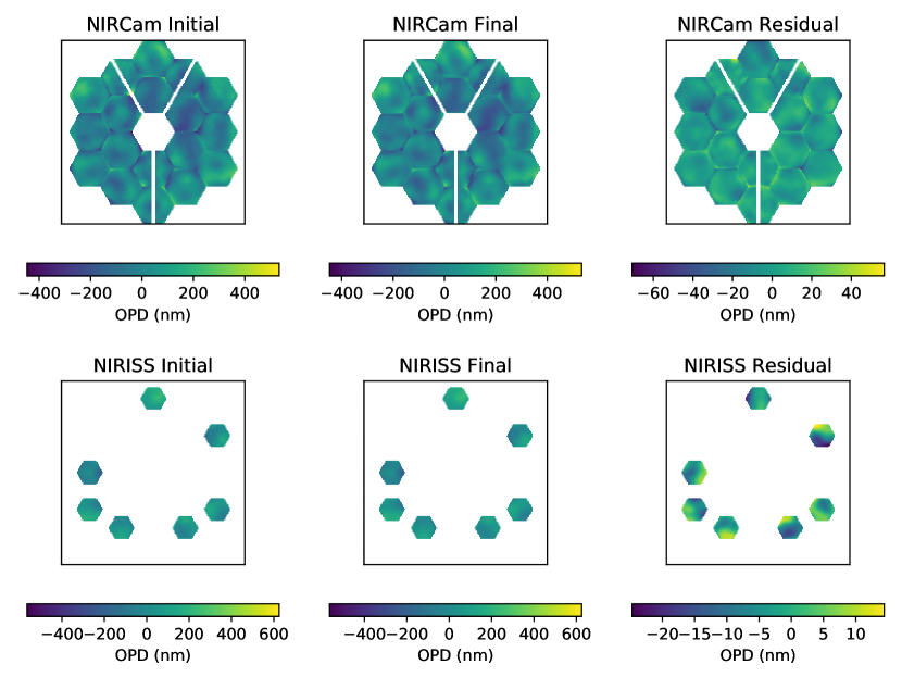
For each pointing, we generate science target and calibrator frames using different optical path difference maps to simulate PSF evolution. We begin by randomly choosing one of ten optical path difference maps included in WebbPSF. We then fit a hexike basis[31] to each mirror segment, including up to 100 coefficients. We evolve each of the hexike coefficients ($C_{n}$) by a factor drawn from a one-mean uniform distribution with a width ($2h$) tuned to result in an rms residual WFEs of $\sim 10$ nm (see Equation 5). This is consistent with the thermal evolution expected for JWST over $\sim$hour long timescales[32].

$$C_{n,seg,cal}=\mathrm{Unif}\left(1-h,1+h\right)C_{n,seg,targ}.$$ (5)

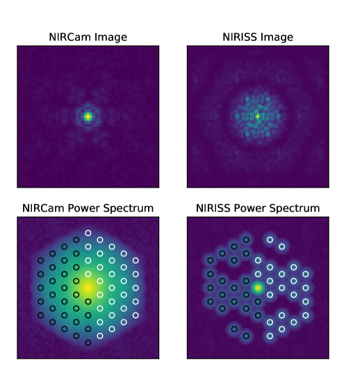
For both NIRCam and NIRISS, this corresponds to $h=0.2$. Figure 4 shows an example initial, final, and residual OPD map for a single simulation for both instruments, and Figure 5 shows example images and power spectra. Figures C.3 and C.4 show histograms of the raw and calibrated NIRCam filled-aperture kernel phases, and NIRISS NRM kernel phases for target stars with apparent M_s band magnitudes of 6.3, and 11.3, respectively.

2.3 Keck OSIRIS

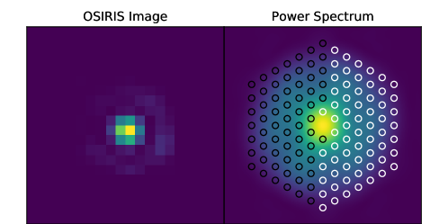
OSIRIS is a K band integral field spectrograph on Keck. We simulate OSIRIS kernel phase observations in the Kn3 bandpass, since it covers the accretion-tracing emission line Br-$\gamma$, which would be of interest for observing protoplanet candidates. This mode contains 433 0.25-nm wavelength bins between 2.121 and 2.229 $\mu$m. With one subaperture per mirror segment it yields 45 kernel phases. We assume 6 hours of available observing time and account for readout, dither, and slew overheads. We optimize our observing strategy in an identical manner to NIRC2, designing visits that either reach the contrast limit or a length of 3 hours including overheads. We keep the peak counts per frame under 30,000 (the OSIRIS saturation limit), and use a readout time of 0.829 seconds per frame, a dither overhead of 6 seconds, and a target acquisition overhead of 90 seconds. We use an OPD evolution prescription identical to NIRC2, and account for detector, sky, and Poisson noise in the same way as for NIRC2. Table 5 lists the relevant detector and noise parameters for OSIRIS, and Table LABEL:tab:osirisobs lists the number of frames and integration times for each target brightness. Figure 6 shows an example image and power spectrum, and Figure C.5 shows kernel phase histograms for targets with K_s band brightnesses of 6 and 11 magnitudes.

Table 5: OSIRIS Noise and Detector Parameters

$\lambda_{c}$   $\mu$m	2.175
$\lambda/D$   (pix)	2.24
S   (mag/arcsec2)	11.2
ZP   (mag)	25.1
DC   (e- / pix / s)	0.035
RN   (e-)	11.0
WD   (DN)	33,000
g   (e-/DN)	4.35

Figure 6: Example simulated OSIRIS image (left) and power spectrum (right).

2.4 JWST NIRSpec

We use the Pandeia engine and WebbPSF software to generate simulated data for NIRSpec IFU observations. We simulate observations for stars with target magnitudes between $\sim 6$ and 13. We use the G395H grating and the F290LP filter, which yield $\gtrsim 4000$ wavelength bins from 2.87 to 5.27 microns. We follow the same methods for OPD evolution and calibration as for NIRCam / NIRISS, evolving the hexike coefficients to achieve 10 nm rms residual OPD ($h=0.11$ in Equation 5). We use the NRSRAPID readout mode.

Since the NIRSpec spaxels are 0.1 arcseconds across they do not Nyquist sample the PSF. We thus generate a nine-point small grid dither for each target observation, with the goal of reconstructing a Nyquist sampled image. To ensure adequate signal to noise for each dither position, we allocate 3 hours for each target and calibrator observation and assume a single observing roll angle. As we did for NIRCam and NIRISS, we find the maximum number of groups ($n_{g}$) that can be included in an integration before saturation. We then split the observations up into nine sets (one for each dither) of $n_{int}$ integrations, each of which has an associated frame-time overhead. Table 6 lists the relevant detector and noise parameters, and LABEL:tab:nirspecobs lists the observing parameters for each target star magnitude.

Table 6: NIRSpec Noise and Detector Parameters

$\lambda_{c}$   $\mu$m	4.07
$\lambda/D$   (pix)	1.29
DC   (e- / pix / s)	0.0092
RN   (e-)	6
WD   (DN)	60,000
g   (e-/DN)	$\sim$ 1

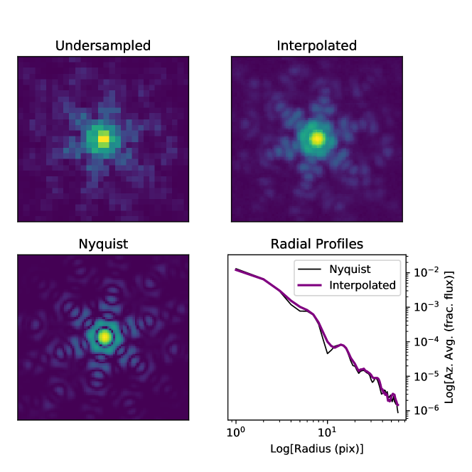
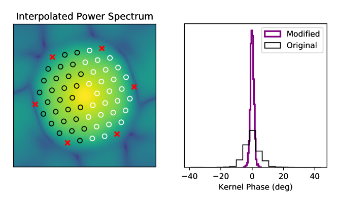
We use the first nine available pointings in the NIRSpec SMALL CYCLING pattern to create a simulated small grid dither. We assign the flux at each pixel in each undersampled image to the angular coordinates located at the center of that pixel. We then use a linear interpolation to assign fluxes to the angular coordinates at the centers of the pixels in the Nyquist sampled image (which have sizes of $\sim 0.03"$) . Figure 7 shows example undersampled and interpolated images, compared to a simulated Nyquist sampled PSF. This interpolation does not account for the spatial extent of each pixel; using a more sophisticated interpolation scheme may improve the results. We also note that up to 60 pointings can be used in the CYCLING pattern, and having more pointings may improve the reconstructed PSF quality. Since the PSF reconstruction is imperfect and some signal is lost on the highest spatial frequencies, we do not include the longest baselines in the kernel phase projection model. This makes the number of observable kernel phases 18. This modified projection degrades the kernel phase effective resolution, but decreases the noise significantly (see Figure 8).

Figure 7: Undersampled (top left), and interpolated (top right) simulated NIRSpec images, with a simulated Nyquist sampled PSF (bottom left) for comparison. The bottom right panel shows the radial profiles for the Nyquist sampled (black, thin line), and the interpolated (purple, thick line) PSF. While similar large-scale changes are seen in both, the interpolated image does not have the same small-scale variations as the Nyquist sampled PSF.

Figure 8: Left: Simulated NIRSpec power spectrum of an interpolated Nyquist sampled image, displayed on a log scale to highlight the features at high spatial frequencies. The hollow circles show the (u,v) sampling points we use to calculate kernel phases. Their histogram is shown in purple in the right panel. The red x’s show the (u,v) points that would have been used for a perfect Nyquist sampled observation, but that we omit from the kernel phase model to reduce the observed scatter. The black histogram shows the kernel phases calculated for a point source when these (u,v) points are included in the kernel phase model. The standard deviations of the purple and black histograms are 1.1^∘ and 5.2 ^∘, respectively.

3 RESULTS: CONTRAST CURVES AND PLANET DETECTION LIMITS

3.1 NIRC2

As a check, we compare the contrast curves for real Keck NRM observations of PSF calibrators to those for simulated observations with the same target star brightness and exposure parameters. The L^′ target star magnitude is 5.8, and the observation consists of a single cube of 20 20-second images. The results are shown in Figure 9; the contrast curves are nearly identical.

Figure 9: Contrast curves for a single target observation made from real L^′ NIRC2 NRM observations (left), and simulated observations (right). The contrast curves are nearly identical, with 5$\sigma$ contrast of $>5.5$ magnitudes.

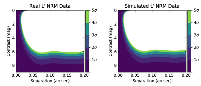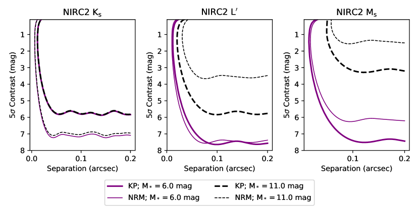
Figure 10 compares the simulated NIRC2 contrast curves for NRM and kernel phase at two representative target brightnesses: apparent magnitudes of 6 and 11. The 6th magnitude case represents the contrast limited regime for K_s and L^′; comparing the NRM and kernel phase contrast curves here shows that kernel phase performance degrades at low Strehl. Kernel phase can achieve comparable contrast to NRM in the bright limit at high ($\gtrsim 0.85$) Strehl. This is evident in the observed kernel phase scatter (see Figure C.1) - the calibrated scatter is much lower for NRM observations at $\mathrm{K_{s}}$ band, but they are comparable at $\mathrm{L^{\prime}}$. When NRM and kernel phase are both in the contrast limit NRM provides slightly higher contrast very close to the core of the PSF (i.e. within $\sim 80$ mas or $\lambda/D$ for the L^′ $\mathrm{M_{*}}=6.0$ contrast curves).

The L^′ contrast curves for the $\mathrm{M_{*}}=11$ star, and all of the M_s contrast curves demonstrate kernel phase and NRM’s different behaviors with the same sky brightness. The NRM PSF is spread over more pixels than the filled-aperture PSF. Thus, contrast degrades more quickly with an increasing sky brightness for NRM observations. This is also apparent in the kernel phase histograms (see Figure C.2); the raw scatter in the L^′ and $\mathrm{M_{s}}$ observations is larger for NRM than for kernel phase. Furthermore, calibration decreases the L^′ kernel phase scatter more significantly for filled aperture observations than for NRM observations. This shows that random noise dominates the NRM observations at lower sky background levels compared to filled-aperture observations.

Figure 10: Kernel phase (thick lines) and NRM (thin lines) for $\mathrm{K_{s}}$ (left), $\mathrm{L^{\prime}}$ (center), and $\mathrm{M_{s}}$ (right) bands. Solid purple lines show observations of 6th apparent magnitude stars, while black dashed lines show 11th apparent magnitude stars.

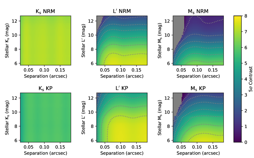
The contrast as a function of stellar apparent magnitude supports these points. Figure 11 shows this: at $\mathrm{K_{s}}$ the achievable contrast is constant with stellar brightness, and higher for NRM than for kernel phase. At L^′, the kernel phase observations stay close to the contrast limit until an apparent magnitude of $\mathrm{L^{\prime}}\sim 9$, while NRM degrades more quickly. Both techniques degrade quickly at M_s, although kernel phase provides higher achievable contrast.

Figure 11: The colorscale shows the 5$\sigma$ single companion contrast for NRM (top) and filled-aperture kernel phase observations (bottom), as a function of target star apparent magnitude and angular separation. Left, center, and right panels show $\mathrm{K_{s}}$, $\mathrm{L^{\prime}}$, and $\mathrm{M_{s}}$ bands, respectively. Grey shaded regions are regions of the parameter space where no companion model was significant at the 5$\sigma$ level, compared to the null (single point source) model. Grey dotted lines contour 1 magnitude increments in contrast.

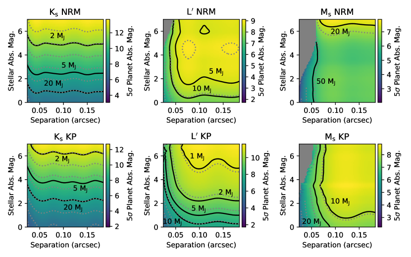
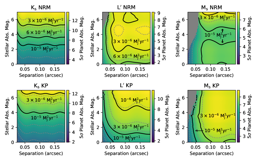
We convert our 5$\sigma$ contrast curves to hot-start planet mass limits using DUSTY models [33], and to planet mass times accretion rate limits using circumplanetary accretion disk models [3, 4]. For the DUSTY models, we assume an age of $\sim 1$ Myr, since the apparent magnitude range we explore corresponds to the absolute magnitudes of $\sim 2$ Myr old stars with masses $\lesssim 5~{}\mathrm{M_{\odot}}$[25] at the distance of Taurus ($\sim 140$ pc[8]). For the circumplanetary accretion disk models, we assume full disks with an inner disk radius of 2 Jupiter radii.[3] Figures 12 and 13 show the planet and accretion disk limits, respectively, for a range of separations and stellar absolute magnitudes assuming a distance of 140 pc. Depending on the stellar magnitude, both NRM and kernel phase at $\mathrm{K_{s}}$ and $\mathrm{L^{\prime}}$ can reach planet masses of a few to a few tens of Jupiter masses, or planet masses times accretion rates of a few times $\sim 10^{-6}$ to $\sim 10^{-5}~{}\mathrm{M_{J}^{2}~{}yr^{-1}}$.

In the bright limit, L^′ NRM and L^′ kernel phase are both sensitive to lower planet masses and accretion rates than $\mathrm{K_{s}}$ NRM. For fainter stars ($\gtrsim$ 10th apparent magnitude or $\gtrsim$5th absolute magnitude), $\mathrm{K_{s}}$ NRM outperforms L^′ NRM due to the higher sky background at L^′. However for these stellar brightnesses, L^′ kernel phase performs best. Despite brighter expected fluxes for hot-start planets at M_s, the high sky background prevents the detection of planets less massive than $\sim 10~{}\mathrm{M_{J}}$. We note that these mass limits look worse for older planets, and for models other than hot-start models. For example, the “warm-start” absolute magnitudes predicted by Spiegel and Burrows (2012)[34] are not detectable even for 1 Myr old 10 $\mathrm{M_{J}}$ planets for either technique or any bandpass.

Figure 12: 5$\sigma$ planet mass limits using 1 Myr DUSTY models (solid lines) for all NIRC2 bandpasses and both techniques. The color scale shows the 5$\sigma$ absolute companion magnitude, calculated using the contrasts shown in Figure 11 and by translating the stellar apparent magnitudes to absolute magnitudes at 140 pc. Grey shaded regions are regions of the parameter space where no companion model was significant at the 5$\sigma$ level, compared to the null (single point source) model. Grey dotted lines contour 1 magnitude increments in planet absolute magnitude. The changing noise regimes (OPD error dominated to random error dominated) in the L^′ and M_s NRM simulations cause the achievable contrast to fall off non-uniformly as the target brightness changes (see Figure 11, upper center and upper right panels). This causes local regions in the L^′ and M_s stellar magnitude - separation parameter space to be better suited for detecting lower planet masses (see upper center and upper right panels here, colorscale and contours)

Figure 13: 5$\sigma$ circumplanetary accretion disk (planet mass times accretion rate) limits (solid lines) for all NIRC2 bandpasses and both techniques. The color scale shows the 5$\sigma$ absolute companion magnitude, calculated using the contrasts shown in Figure 11 and by translating the stellar apparent magnitudes to absolute magnitudes at 140 pc. Grey shaded regions are regions of the parameter space where no companion model was significant at the 5$\sigma$ level, compared to the null (single point source) model. Grey dotted lines contour 1 magnitude increments in planet absolute magnitude. The changing noise regimes (OPD error dominated to random error dominated) in the L^′ and M_s NRM simulations cause the achievable contrast to fall off non-uniformly as the target brightness changes (see Figure 11, upper center and upper right panels). This causes local regions in the L^′ and M_s stellar magnitude - separation parameter space to be better suited for detecting lower planet masses times accretion rates (see upper center and upper right panels here, colorscale and contours).

3.2 JWST: NIRCam Kernel Phase and NIRISS Aperture Masking Interferometry

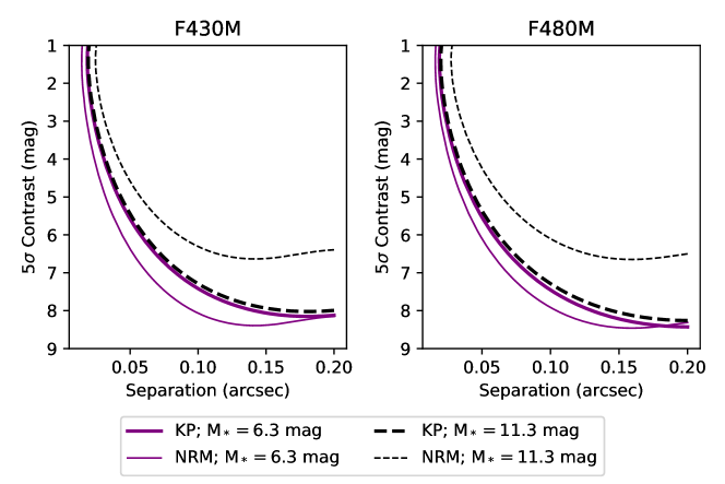
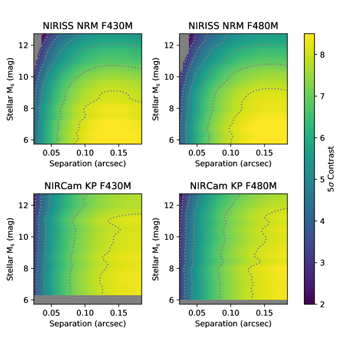
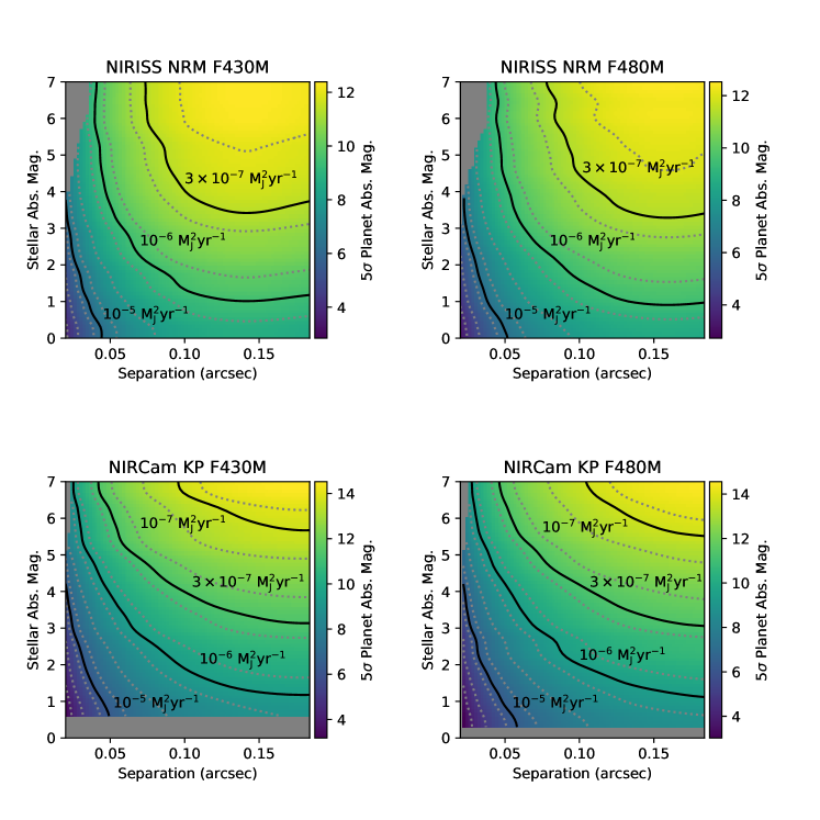
Figure 14 shows representative contrast curves for $\mathrm{M_{*}}=6.3$ and $\mathrm{M_{*}}=11.3$ apparent magnitude stars for NIRCam and NIRISS. Again, in the bright limit ($\mathrm{M_{*}}=6.3$), NRM outperforms kernel phase within $\lambda/D$ ($\sim 150$ mas), by $0.5-1.0$ magnitudes. At larger separations, kernel phase provides comparable contrast. The faint $\mathrm{M_{*}}=11.3$ mag contrast curves show that at lower signal to noise NIRCam kernel phase can provide higher contrast than NRM on NIRISS. Figures C.3 and C.4 support this. The raw and calibrated kernel phase scatters for NIRCam and NIRISS are comparable in the bright case, but in the faint case the NIRCam kernel phases calibrate to a lower noise level than the NIRISS kernel phases. This is apparent in Figure 15, which shows that NIRISS’s contrast falls off as the stellar apparent magnitude becomes greater than $\sim 9$, but NIRCam’s contrast does not. We also note that for apparent magnitudes less than $\sim 6-6.5$, NIRCam is at its saturation limit and thus kernel phase cannot be used.

Figure 14: NIRCam kernel phase (thick lines) and NIRISS NRM (thin lines) for F430M (left) and F480M (right) bands. Solid purple lines show observations of 6.3 apparent magnitude stars, while black dashed lines show 11.3 apparent magnitude stars.

Figure 15: The colorscale shows the 5$\sigma$ single companion contrast for NIRISS NRM (top) and NIRCam filled-aperture kernel phase observations (bottom), as a function of target star apparent magnitude and angular separation. The grey dotted lines show 1 magnitude increments in companion contrast. Left and right panels show F430M and F480M bands, respectively. Grey shaded regions are regions of the parameter space where either no companion model was significant at the 5$\sigma$ level, compared to the null (single point source) model, or regions where the target magnitude was below the bright limit. Grey dotted lines contour 1 magnitude increments in contrast.

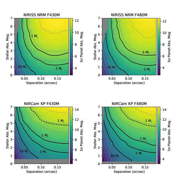
Figures 16 - 17 show the 5$\sigma$ planet and circumplanetary accretion disk limits for a range of stellar absolute magnitudes and angular separations. The absolute magnitudes were calculated assuming a distance of 140 pc. The greater stability of JWST leads to higher contrast than that achieved with NIRC2, making lower mass planets and lower accretion rates more accessible for brighter stars. Planet masses of 1$\mathrm{M_{J}}$ are detectable for more than half the stellar absolute magnitudes in the hot-start case, and for the high stellar absolute magnitudes in the warm-start case for NIRCam. The range of detectable planet masses times accretion rates reaches below $10^{-7}~{}\mathrm{M_{J}^{2}~{}yr^{-1}}$. Comparing the top and bottom panels of Figures 16 – 17 shows that, with NIRISS NRM in the bright limit ($\mathrm{M_{abs}}\lesssim 2-3$), slightly lower mass (accretion rate) planets can be detected at smaller angular separations. The maximum detectable absolute planet magnitude is higher for NIRCam, as a result of the improved contrast for fainter stars; this is particularly useful for detecting planets that have formed via non-hot-start scenarios.

Figure 16: 5$\sigma$ planet mass limits using 1 Myr DUSTY models (solid lines) and 1 Myr warm-start Spiegel and Burrows (2012) models (dashed lines) for the F430M and F480M bandpasses and both techniques / instruments. The color scale shows the 5$\sigma$ absolute companion magnitude, calculated using the contrasts shown in Figure 15 and by translating the stellar apparent magnitudes to absolute magnitudes at 140 pc. The grey dotted lines show 1 magnitude increments in planet absolute magnitude. For clarity, since the 1 Myr warm-start models are tightly clustered in absolute magnitude, we only contour the 1 $\mathrm{M_{J}}$ model. Warm-start planets with masses less than $10~{}\mathrm{M_{J}}$ are only detectable in the NIRCam observations for high stellar absolute magnitudes. Grey shaded regions are regions of the parameter space where either no companion model was significant at the 5$\sigma$ level, compared to the null (single point source) model, or regions where the target magnitude was below the bright limit.

Figure 17: 5$\sigma$ circumplanetary accretion disk (planet mass times accretion rate) limits (solid lines) for all NIRC2 bandpasses and both techniques. The color scale shows the 5$\sigma$ absolute companion magnitude, calculated using the contrasts shown in Figure 15 and by translating the stellar apparent magnitudes to absolute magnitudes at 140 pc. The grey dotted lines show 1 magnitude increments in planet absolute magnitude. Grey shaded regions are regions of the parameter space where either no companion model was significant at the 5$\sigma$ level, compared to the null (single point source) model, or regions where the target magnitude was below the bright limit.

3.3 Keck OSIRIS

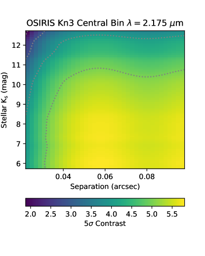
Figure 18 shows the achievable kernel phase contrast for OSIRIS as a function of $\mathrm{K_{s}}$ stellar apparent magnitude for the central wavelength bin in the Kn3 bandpass ($\lambda=2.175~{}\mu$m). Contrasts of $\sim 5$ magnitudes are detectable at the $5\sigma$ level. This is lower than the achievable contrast for NIRC2 at broadband $\mathrm{K_{s}}$, and the calibrated kernel phase scatter is also higher for OSIRIS (see Figure C.5) for target stars with the same brightness. This may be due to the fact that a single OSIRIS wavelength bin has 1700 times lower throughput than NIRC2: random noise sources from the sky and detector may be a more significant noise source for OSIRIS, degrading contrast.

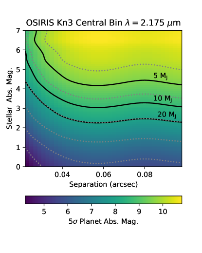
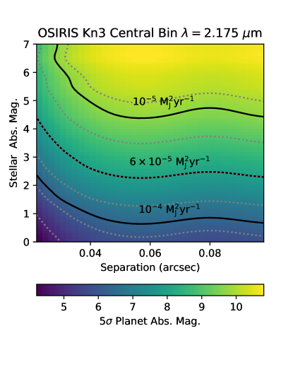
Figures 19 and 20 translate these contrast limits to planet mass limits as a function of stellar absolute magnitude. We again assume a distance of 140 pc. With OSIRIS, planet masses of $5-20~{}\mathrm{M_{J}}$ are detectable for stellar absolute magnitudes greater than $\sim 2$. Warm start models with masses less than $10~{}\mathrm{M_{J}}$ are not detectable. Planet masses times accretion rates of $\sim 10^{-5}~{}\mathrm{M_{J}^{2}~{}yr^{-1}}$ are detectable for the fainter stars ($\mathrm{K_{s}}\sim 10$; $\mathrm{M_{K_{s}}}\sim 5$). We note that these detection limits would be worse for the shortest wavelength bin ($\lambda=2.121~{}\mu$m) and better for the longest wavelength bin ($\lambda=2.229~{}\mu$m) due to the wavelength dependence of the Strehl ratio.

Figure 18: The colorscale shows the 5$\sigma$ single companion contrast for OSIRIS kernel phase observations as a function of target star apparent magnitude and angular separation. Grey dotted lines contour 1 magnitude increments in contrast.

Figure 19: 5$\sigma$ planet mass limits using 1 Myr DUSTY models (solid lines) for OSIRIS kernel phase. The color scale shows the 5$\sigma$ absolute companion magnitude, calculated using the contrasts shown in Figure 18 and by translating the stellar apparent magnitudes to absolute magnitudes at 140 pc. Grey dotted lines contour 1 magnitude increments in planet absolute magnitude.

Figure 20: 5$\sigma$ circumplanetary accretion disk (planet mass times accretion rate) limits (solid lines) for OSIRIS. The color scale shows the 5$\sigma$ absolute companion magnitude, calculated using the contrasts shown in Figure 18 and by translating the stellar apparent magnitudes to absolute magnitudes at 140 pc. Grey dotted lines contour 1 magnitude increments in planet absolute magnitude.

3.4 JWST NIRSpec

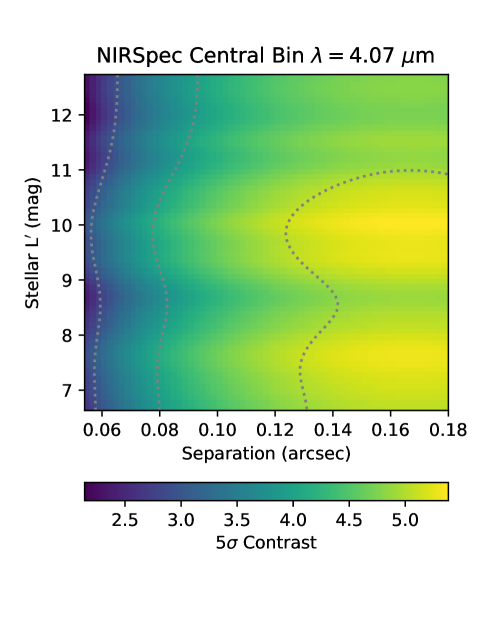
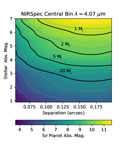
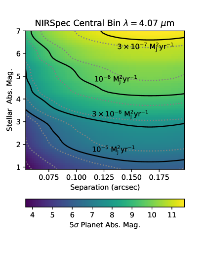
Figure 21 shows the achievable kernel phase contrast for JWST NIRSpec as a function of $\mathrm{L^{\prime}}$ stellar apparent magnitude for the central wavelength bin ($\lambda=4.07~{}\mu$m), and Figure C.6 shows example histograms of the raw and calibrated kernel phases. Contrasts of $\sim 5$ magnitudes are detectable at the $5\sigma$ level for all target star magnitudes. Figures 22 and 23 translate these contrast limits to planet mass limits as a function of stellar absolute magnitude, assuming a distance of 140 pc. With NIRSpec, planet masses of a few $\mathrm{M_{J}}$ are detectable for stellar absolute magnitudes greater than $\sim 4-5$. Warm start models with masses less than $10~{}\mathrm{M_{J}}$ are not detectable. Planet masses times accretion rates of $\sim 10^{-5}~{}\mathrm{M_{J}^{2}~{}yr^{-1}}$ are detectable for all target star absolute magnitudes, and lower accretion rates $\sim$ a few times $10^{-7}~{}\mathrm{M_{J}^{2}~{}yr^{-1}}$ to $\sim 10^{-6}~{}\mathrm{M_{J}^{2}~{}yr^{-1}}$ are detectable for stars with absolute magnitudes greater than $\sim 5$. We note that these detection limits would be worse for the shortest wavelength bin ($\lambda=2.87~{}\mu$m), partly due to lower Strehl, and partly due to the fact that the PSF is more poorly sampled in this wavelength bin. They would be better for the longest wavelength bin ($\lambda=5.27~{}\mu$m) where the Strehl is higher and the PSF is larger.

Figure 21: The colorscale shows the 5$\sigma$ single companion contrast for NIRSpec kernel phase observations as a function of target star apparent magnitude and angular separation. Grey dotted lines show 1 magnitude increments in contrast.

Figure 22: 5$\sigma$ planet mass limits using 1 Myr DUSTY models (solid lines) for NIRSpec kernel phase. The color scale shows the 5$\sigma$ absolute companion magnitude, calculated using the contrasts shown in Figure 21 and by translating the stellar apparent magnitudes to absolute magnitudes at 140 pc. Grey dotted lines show 1 magnitude increments in planet absolute magnitude.

Figure 23: 5$\sigma$ circumplanetary accretion disk (planet mass times accretion rate) limits (solid lines) for NIRSpec kernel phase. The color scale shows the 5$\sigma$ absolute companion magnitude, calculated using the contrasts shown in Figure 21 and by translating the stellar apparent magnitudes to absolute magnitudes at 140 pc. Grey dotted lines show 1 magnitude increments in planet absolute magnitude.

4 DISCUSSION

The contrast curves and derived planet mass / accretion rate limits for NIRC2, NIRCam, and NIRISS show that filled-aperture kernel phase is a viable alternative to non-redundant masking for high Strehl ($\sim 0.8-0.9$) observations. This corresponds to wavelengths redder than $\sim 3.8$ microns for ground-based observations. At these wavelengths, the sky brightness is a lesser problem for kernel phase observations, since the NRM point spread function is spread out over more pixels than the filled-aperture PSF. Space based observations with a thermal background would also benefit from kernel phase for the same reason. The simulations demonstrated this: filled-aperture kernel phase provided lower noise levels and thus better planet mass / accretion rate limits for faint stars (apparent magnitude $\gtrsim 8$ mag for NIRC2 L^′, and apparent magnitude $\gtrsim 9-10$ for JWST NIRCam and NIRISS). For both Keck and JWST in the bright limit (apparent magnitude $\sim 6$), kernel phase can achieve comparable contrast to NRM at separations outside $\lambda/D$. However, at angular separations within $\lambda/D$, non-redundant masking provided slightly higher contrast ($\sim 0.5-1$ mag) than filled-aperture kernel phase.

While NRM can provide slightly higher contrast close-in, the required integration times are much longer - a factor of $\sim 10$ to achieve similar signal to noise as kernel phase. With limited observing resources, using kernel phase for stars that are faint compared to the thermal background would save time. This would be useful in the context of a large survey for young planets, since the two techniques can place similar constraints on (accreting) planet populations in the contrast limit, with kernel phase outperforming NRM when the sky background becomes significant. NRM’s better performance close to the PSF core in the contrast limit suggests that an intermediate case such as a redundant mask may be the ideal observing setup for carrying out faster observations without a loss in contrast in the bright limit.

The OSIRIS and NIRSpec simulations show that kernel phase on an IFS can reach contrasts of $5-6$ magnitudes. This is an exciting mode for characterizing young planets at smaller angular separation than that typically achieved with an IFS. For fully-formed planets, this will lead to better atmospheric constraints than possible with narrowband imaging.[1] For accreting planets, it will help to distinguish between different formation scenarios: e.g. hot-start versus circumplanetary disk accretion.[4, 3, 16] The single-bin contrast curves show that kernel phase on an integral field spectrograph is capable of simultaneous detection and characterization; individual wavelength bins can be treated independently.

The broadband simulations show an improvement in both achievable contrast and planet mass / accretion rate limits at L^′ compared to Ks. This suggests that a mid-infrared integral field spectrograph would be particularly useful for planet characterization with these techniques. Arizona Lenslets for Exoplanet Spectroscopy (ALES)[35] on the Large Binocular Telescope is a $3-5~{}\mu$m integral field spectrograph with a non-redundant masking mode. ALES provides a spectral resolution of R$\sim$20, and the non-redundant mask has 6 holes with a maximum baseline of 8 meters in single-aperture mode, and 12 holes with a maximum baseline of 23 meters in dual-aperture mode. ALES’ redder wavelength range should lead to higher contrast (and lower planet mass / accretion rate limits) compared to shorter-wavelength ground-based integral field spectrographs. ALES has not yet been characterized for non-redundant masking or filled-aperture kernel phase observations; this will be the subject of future work.

Current ground based observations can only reach planet masses of several Jupiter masses, and planet masses times accretion rates of a few times $\sim 10^{-6}$ to $\sim 10^{-5}~{}\mathrm{M_{J}^{2}~{}yr^{-1}}$. Furthermore, the resolution limit of $8-10$ meter class telescopes means that they can only probe spatial separations of $\gtrsim 10$ AU in the near- to mid-infrared. Both of these limits will improve as the next generation of extremely large telescopes comes online; building signal to noise on faint stars will take less time, and the factor of $\sim 3$ boost in resolution will probe spatial scales of a few AU. The 23-meter baseline dual-aperture Large Binocular Telescope can achieve similar resolution now and has an NRM mode, which has been demonstrated to work even without operational co-phasing[18]. NRM and kernel phase on LBT could produce ELT-like planet detections before the ELTs are operational, and allow us to develop these tools for use on the next generation of telescopes.

Both NRM and filled-aperture kernel phase on James Webb will expand the planet detection parameter space beyond that of ground-based observations. While JWST will not have higher resolution than current ground-based facilities, its greater stability will lead to lower kernel phase scatter and provide higher contrast. Furthermore, it will not have the same limitations on target star brightness as an AO-corrected telescope. These factors combined mean that JWST will detect and characterize lower mass / accretion rate planets than we can observe from the ground.

5 CONCLUSIONS

We presented contrast curves for non-redundant masking and filled-aperture kernel phase on several broadband imagers and integral field spectrographs. The observations were simulated to carefully control noise sources, and when possible we used real observations to anchor our OPD prescription. The simulated contrast curves show that for high Strehl, kernel phase performs comparably to or better than NRM outside of $\lambda/D$. The compactness of the kernel phase PSF makes it particularly well suited for low SNR observations where random noise sources dominate. In the contrast limited regime, masking outperforms filled-aperture kernel phase by $0.5-1$ magnitudes within the diffraction limit. This slightly lower contrast suggests that in the bright limit, redundant masks may be a good compromise to reach high contrast with shorter exposure times than NRM.

Both NRM and kernel phase are capable of detecting giant, recently-formed planets and accretion signatures from forming planets. Filled-aperture kernel phase, applied on an integral field spectrograph, will be capable of simultaneous detection and characterization, and will reach smaller separations than traditional IFS high contrast imaging. Both techniques, applied on the next generation of adaptive optics systems and space- and ground-based observing facilities, will expand the planet detection parameter space in volume, semi-major axis, and contrast. This will greatly inform our understanding of planet formation and evolution.

Disclosures

The authors have no relevant financial interests in the manuscript and no other potential conflicts of interest to disclose.

Appendix A Kernel Phase Projection and Weighting

A.1 Projection

We use the “Martinache” projection[12] to calculate kernel phases; this forms orthonormal combinations of Fourier phases that eliminate instrumental phase. The projection is based on representing Fourier phases as linear combinations of pupil plane phases:

$$\Phi=\mathrm{R^{-1}}\cdot\mathrm{A}\cdot\phi+\Phi_{0},$$ (6)

where $\Phi$ represents a vector of Fourier phases with length M, R is a diagonal matrix containing the redundancy of each kernel phase, A is a matrix that describes how pupil plane phases ($\phi$) are combined to create Fourier phases, and $\Phi_{0}$ is a vector of Fourier phases that are intrinsic to the source. The kernel of $\mathrm{R^{-1}\cdot A}$, $\mathrm{K}$,[36] found using singular value decomposition, projects Fourier phases into kernel phases and eliminates the instrumental phase term, $\phi$. The matrix $\mathrm{K}$ is analogous to the closure phase projection in interferometric observations, but is not restricted to values of only 0, 1, and -1.

A.2 Weighted Averaging

In interferometric observations, closure phases are calculated from bispectra, the product of three complex visibilities on baselines forming a triangle [10]. When closure phases are calculated for a cube of images, the bispectra are averaged over the cube, and the phase of the average bispectrum is taken as the average closure phase [37]. Averaging bispectra rather than phases has been demonstrated to perform better in noisy conditions[38]. We thus generalize this form of vector averaging, which upweights higher signal to noise observations by including amplitude information in the average, from closure phase to kernel phase.

For each frame, for the $i^{th}$ kernel phase, we calculate a complex quantity by taking a weighted product of complex visibilities:

$$\prod_{j=1}^{M}V_{j}^{K_{i,j}},$$ (7)

where $K_{i,j}$ is value in the $i^{th}$ row and $j^{th}$ column of the kernel phase projection matrix, $j$ is the index that describes the M Fourier phases, and $V_{j}$ is the $j^{th}$ complex visibility, which has both amplitude and phase. The average kernel phase over a cube of $n_{im}$ images is then:

$$\mathrm{Arg}\left(\frac{1}{n_{im}}\sum_{k=1}^{n_{im}}\prod_{j=1}^{M}V_{j}^{K_{i,j}}\right).$$ (8)

This ensures that the Fourier phases are combined using the weights contained in the matrix K, but that amplitude information is used to weight the kernel phases by signal-to-noise when averaging them over multiple frames. We checked that this weighting scheme performs similarly or better than averaging kernel phases themselves for individual frames, depending on the noise regime.

Appendix B Simulated Observation Planning

Target apparent magnitude

Total number of coadds per visit

Total number of frames per visit

Total number of dithers per visit

Integration time per coadd

Exposure time per visit

Total observing time (including overheads) per visit

Number of science target visits in one half night

Observing efficiency (exposure time divided by total observing time)

Table B.1: NIRC2 Ks NRM Observation Details

Ks (mag)	$n_{coadds}$	$n_{frames}$	$n_{dit}$	$t_{coadd}$	$t_{exp}$	$t_{tot}$	$n_{vis}$	$eff$
5.7	3877	9	2	0.0453	175	491	22	0.36
5.8	3662	10	2	0.0502	184	491	22	0.37
5.9	3487	10	2	0.0553	193	491	22	0.39
6.0	3329	10	2	0.0603	201	491	22	0.41
6.1	3033	11	2	0.0703	213	491	22	0.43
6.2	2912	11	2	0.0753	219	491	22	0.45
6.3	2783	12	2	0.0803	224	491	22	0.46
6.4	2584	12	2	0.0904	234	491	22	0.48
6.5	2399	12	2	0.1012	243	491	22	0.49
6.6	2247	13	2	0.1105	248	491	22	0.51
6.7	2115	13	2	0.1205	255	491	22	0.52
6.8	1998	13	2	0.1305	261	491	22	0.53
6.9	1833	14	2	0.1455	267	491	22	0.54
7.0	1743	14	2	0.1556	271	491	22	0.55
7.1	1624	14	2	0.1707	277	491	22	0.56
7.2	1480	15	2	0.1907	282	491	22	0.57
7.3	1393	15	2	0.2057	287	491	22	0.58
7.4	1292	15	2	0.2257	292	491	22	0.59
7.5	1184	15	2	0.2509	297	491	22	0.61
7.6	1110	15	2	0.2709	301	491	22	0.61
7.7	1008	16	2	0.3012	304	491	22	0.62
7.8	941	16	2	0.3262	307	491	22	0.63
7.9	861	16	2	0.3612	311	491	22	0.63
8.0	793	16	2	0.3964	314	491	22	0.64
8.1	735	16	2	0.4317	317	491	22	0.65
8.2	672	16	2	0.4768	320	491	22	0.65
8.3	615	16	2	0.5257	323	491	22	0.66
8.4	566	17	2	0.5716	324	491	22	0.66
8.5	519	17	2	0.6279	326	491	22	0.66
8.6	477	17	2	0.6876	328	491	22	0.67
8.7	438	17	2	0.7533	330	491	22	0.67
8.8	403	17	2	0.8231	332	491	22	0.68
8.9	369	17	2	0.9035	333	491	22	0.68
9.0	337	17	2	0.9941	335	491	22	0.68
9.1	309	17	2	1.0887	336	491	22	0.69
9.2	283	17	2	1.1933	338	491	22	0.69
9.3	258	17	2	1.3138	339	491	22	0.69
9.4	237	17	2	1.4346	340	491	22	0.69
9.5	217	17	2	1.5714	341	491	22	0.69
9.6	198	17	2	1.727	342	491	22	0.7
9.7	180	17	2	1.9047	343	491	22	0.7
9.8	164	17	2	2.0954	344	491	22	0.7
9.9	150	17	2	2.2957	344	491	22	0.7
10.0	137	17	2	2.5182	345	491	22	0.7
10.1	125	17	2	2.7648	346	491	22	0.7
10.2	115	18	2	2.9906	344	491	22	0.7
10.3	105	18	2	3.2802	344	491	22	0.7
10.4	96	18	2	3.5924	345	491	22	0.7
10.5	87	18	2	3.9692	345	491	22	0.7
10.6	80	18	2	4.3209	346	491	22	0.7
10.7	73	18	2	4.74	346	491	22	0.7
10.8	66	18	2	5.248	346	491	22	0.71
10.9	61	18	2	5.6823	347	491	22	0.71
11.0	55	18	2	6.3076	347	491	22	0.71
11.1	50	18	2	6.9434	347	491	22	0.71
11.2	46	18	2	7.5515	347	491	22	0.71
11.3	42	18	2	8.2755	348	491	22	0.71
11.4	38	18	2	9.1518	348	491	22	0.71
11.5	35	18	2	9.9405	348	491	22	0.71
11.6	17	17	2	20.647	351	491	22	0.71
11.7	17	17	2	20.647	351	491	22	0.71
11.8	17	17	2	20.647	351	491	22	0.71
11.9	17	17	2	20.647	351	491	22	0.71
12.0	17	17	2	20.647	351	491	22	0.71
12.1	17	17	2	20.647	351	491	22	0.71
12.2	17	17	2	20.647	351	491	22	0.71
12.3	17	17	2	20.647	351	491	22	0.71
12.4	17	17	2	20.647	351	491	22	0.71
12.5	17	17	2	20.647	351	491	22	0.71
12.6	17	17	2	20.647	351	491	22	0.71
12.7	17	17	2	20.647	351	491	22	0.71

Target apparent magnitude

Total number of coadds per visit

Total number of frames per visit

Total number of dithers per visit

Integration time per coadd

Exposure time per visit

Total observing time (including overheads) per visit

Number of science target visits in one half night

Observing efficiency (exposure time divided by total observing time)

Table B.2: NIRC2 Kp NRM Observation Details

Ks (mag)	$n_{coadds}$	$n_{frames}$	$n_{dit}$	$t_{coadd}$	$t_{exp}$	$t_{tot}$	$n_{vis}$	$eff$
5.7	6975	2	2	0.0051	36	491	22	0.07
5.8	6975	2	2	0.0051	36	491	22	0.07
5.9	6975	2	2	0.0051	36	491	22	0.07
6.0	6321	4	2	0.0101	64	491	22	0.13
6.1	6321	4	2	0.0101	64	491	22	0.13
6.2	6321	4	2	0.0101	64	491	22	0.13
6.3	6321	4	2	0.0101	64	491	22	0.13
6.4	6321	4	2	0.0101	64	491	22	0.13
6.5	6321	4	2	0.0101	64	491	22	0.13
6.6	5801	5	2	0.0152	88	491	22	0.18
6.7	5801	5	2	0.0152	88	491	22	0.18
6.8	5801	5	2	0.0152	88	491	22	0.18
6.9	5801	5	2	0.0152	88	491	22	0.18
7.0	5356	6	2	0.0202	108	491	22	0.22
7.1	5356	6	2	0.0202	108	491	22	0.22
7.2	4969	7	2	0.0252	125	491	22	0.26
7.3	4969	7	2	0.0252	125	491	22	0.26
7.4	4969	7	2	0.0252	125	491	22	0.26
7.5	4659	7	2	0.0302	141	491	22	0.29
7.6	4359	8	2	0.0352	154	491	22	0.31
7.7	4359	8	2	0.0352	154	491	22	0.31
7.8	4093	9	2	0.0402	165	491	22	0.34
7.9	3877	9	2	0.0453	175	491	22	0.36
8.0	3662	10	2	0.0502	184	491	22	0.37
8.1	3662	10	2	0.0502	184	491	22	0.37
8.2	3487	10	2	0.0553	193	491	22	0.39
8.3	3165	11	2	0.0653	207	491	22	0.42
8.4	3033	11	2	0.0703	213	491	22	0.43
8.5	2912	11	2	0.0753	219	491	22	0.45
8.6	2680	12	2	0.0854	229	491	22	0.47
8.7	2584	12	2	0.0904	234	491	22	0.48
8.8	2399	12	2	0.1012	243	491	22	0.49
8.9	2247	13	2	0.1105	248	491	22	0.51
9.0	2115	13	2	0.1205	255	491	22	0.52
9.1	1998	13	2	0.1305	261	491	22	0.53
9.2	1833	14	2	0.1455	267	491	22	0.54
9.3	1702	14	2	0.1606	273	491	22	0.56
9.4	1588	14	2	0.1757	279	491	22	0.57
9.5	1480	15	2	0.1907	282	491	22	0.57
9.6	1366	15	2	0.2108	288	491	22	0.59
9.7	1268	15	2	0.2309	293	491	22	0.6
9.8	1184	15	2	0.2509	297	491	22	0.61
9.9	1090	15	2	0.2768	302	491	22	0.61
10.0	1008	16	2	0.3012	304	491	22	0.62
10.1	929	16	2	0.3311	308	491	22	0.63
10.2	861	16	2	0.3612	311	491	22	0.63
10.3	793	16	2	0.3964	314	491	22	0.64
10.4	728	16	2	0.4363	318	491	22	0.65
10.5	672	16	2	0.4768	320	491	22	0.65
10.6	615	16	2	0.5257	323	491	22	0.66
10.7	566	17	2	0.5716	324	491	22	0.66
10.8	519	17	2	0.6279	326	491	22	0.66
10.9	477	17	2	0.6876	328	491	22	0.67
11.0	435	17	2	0.7588	330	491	22	0.67
11.1	401	17	2	0.8274	332	491	22	0.68
11.2	367	17	2	0.9087	333	491	22	0.68
11.3	335	17	2	1.0003	335	491	22	0.68
11.4	307	17	2	1.0961	336	491	22	0.69
11.5	281	17	2	1.2021	338	491	22	0.69
11.6	258	17	2	1.3138	339	491	22	0.69
11.7	236	17	2	1.4409	340	491	22	0.69
11.8	215	17	2	1.5865	341	491	22	0.69
11.9	197	17	2	1.736	342	491	22	0.7
12.0	179	17	2	1.9156	343	491	22	0.7
12.1	164	18	2	2.0821	341	491	22	0.7
12.2	150	18	2	2.2811	342	491	22	0.7
12.3	137	18	2	2.5023	343	491	22	0.7
12.4	125	18	2	2.7474	343	491	22	0.7
12.5	114	18	2	3.0173	344	491	22	0.7
12.6	104	18	2	3.3122	344	491	22	0.7
12.7	95	18	2	3.6307	345	491	22	0.7

Target apparent magnitude

Total number of coadds per visit

Total number of frames per visit

Total number of dithers per visit

Integration time per coadd

Exposure time per visit

Total observing time (including overheads) per visit

Number of science target visits in one half night

Observing efficiency (exposure time divided by total observing time)

Table B.3: NIRC2 L^′ NRM Observation Details

L′ (mag)	$n_{coadds}$	$n_{frames}$	$n_{dit}$	$t_{coadd}$	$t_{exp}$	$t_{tot}$	$n_{vis}$	$eff$
5.7	1702	14	2	0.1606	273	491	22	0.56
5.8	1662	14	2	0.1656	275	491	21	0.56
5.9	1588	14	2	0.1757	279	491	22	0.57
6.0	1513	14	2	0.1869	283	491	22	0.58
6.1	1480	15	2	0.1907	282	491	22	0.57
6.2	1421	15	2	0.2007	285	491	22	0.58
6.3	1393	15	2	0.2057	287	491	22	0.58
6.4	1340	15	2	0.2158	289	491	22	0.59
6.5	1315	15	2	0.2209	290	491	22	0.59
6.6	1268	15	2	0.2309	293	491	22	0.6
6.7	1246	15	2	0.2359	294	491	22	0.6
6.8	1225	15	2	0.2408	295	491	22	0.6
6.9	1184	15	2	0.2509	297	491	22	0.61
7.0	1164	15	2	0.256	298	491	22	0.61
7.1	1146	15	2	0.2608	299	491	22	0.61
7.2	1127	15	2	0.2661	300	491	22	0.61
7.3	1110	15	2	0.2709	301	491	22	0.61
7.4	1071	16	2	0.2806	300	491	22	0.61
7.5	1071	16	2	0.2806	300	491	22	0.61
7.6	1054	16	2	0.2859	301	491	22	0.61
7.7	1038	16	2	0.2911	302	491	22	0.62
7.8	1023	16	2	0.2961	303	491	22	0.62
7.9	1008	16	2	0.3012	304	491	22	0.62
8.0	1153	18	2	0.3205	370	568	19	0.65
8.1	1386	22	3	0.3245	450	675	16	0.67
8.2	1639	26	3	0.3202	525	771	14	0.68
8.3	1970	31	4	0.3147	620	900	12	0.69
8.4	2330	37	4	0.33	769	1080	10	0.71
8.5	2801	45	5	0.3541	992	1350	8	0.73
8.6	3315	54	6	0.3419	1133	1543	7	0.73
8.7	3984	64	7	0.3337	1329	1800	6	0.74
8.8	4716	77	8	0.3432	1618	2160	5	0.75
8.9	5669	93	10	0.3641	2064	2700	4	0.76
9.0	6815	111	12	0.419	2855	3600	3	0.79
9.1	8068	134	14	0.3384	2730	3600	3	0.76
9.2	9699	161	17	0.4508	4372	5400	2	0.81
9.3	11660	193	20	0.359	4186	5400	2	0.78
9.4	13808	232	24	0.6786	9370	10800	1	0.87
9.5	16600	279	28	0.5484	9104	10800	1	0.84
9.6	19956	335	34	0.4399	8778	10800	1	0.81
9.7	23991	402	41	0.3496	8388	10800	1	0.78
9.8	24711	414	49	0.335	8278	10800	1	0.77
9.9	24623	413	55	0.335	8249	10800	1	0.76
10.0	24302	414	55	0.34	8262	10800	1	0.77
10.1	24302	414	55	0.34	8262	10800	1	0.77
10.2	24302	414	55	0.34	8262	10800	1	0.77
10.3	24302	414	55	0.34	8262	10800	1	0.77
10.4	24302	414	55	0.34	8262	10800	1	0.77
10.5	24302	414	55	0.34	8262	10800	1	0.77
10.6	24302	414	55	0.34	8262	10800	1	0.77
10.7	24302	414	55	0.34	8262	10800	1	0.77
10.8	24302	414	55	0.34	8262	10800	1	0.77
10.9	24302	414	55	0.34	8262	10800	1	0.77
11.0	24004	415	54	0.345	8281	10800	1	0.77
11.1	24004	415	54	0.345	8281	10800	1	0.77
11.2	24004	415	54	0.345	8281	10800	1	0.77
11.3	24004	415	54	0.345	8281	10800	1	0.77
11.4	24004	415	54	0.345	8281	10800	1	0.77
11.5	24004	415	54	0.345	8281	10800	1	0.77
11.6	24004	415	54	0.345	8281	10800	1	0.77
11.7	24004	415	54	0.345	8281	10800	1	0.77
11.8	24004	415	54	0.345	8281	10800	1	0.77
11.9	24004	415	54	0.345	8281	10800	1	0.77
12.0	24004	415	54	0.345	8281	10800	1	0.77
12.1	24004	415	54	0.345	8281	10800	1	0.77
12.2	24004	415	54	0.345	8281	10800	1	0.77
12.3	24004	415	54	0.345	8281	10800	1	0.77
12.4	24004	415	54	0.345	8281	10800	1	0.77
12.5	24004	415	54	0.345	8281	10800	1	0.77
12.6	24004	415	54	0.345	8281	10800	1	0.77
12.7	24004	415	54	0.345	8281	10800	1	0.77

Target apparent magnitude

Total number of coadds per visit

Total number of frames per visit

Total number of dithers per visit

Integration time per coadd

Exposure time per visit

Total observing time (including overheads) per visit

Number of science target visits in one half night

Observing efficiency (exposure time divided by total observing time)

Table B.4: NIRC2 L^′ KP Observation Details

L′ (mag)	$n_{coadds}$	$n_{frames}$	$n_{dit}$	$t_{coadd}$	$t_{exp}$	$t_{tot}$	$n_{vis}$	$eff$
5.7	4659	7	2	0.0302	141	491	22	0.29
5.8	4359	8	2	0.0352	154	491	22	0.31
5.9	4093	9	2	0.0402	165	491	22	0.34
6.0	4093	9	2	0.0402	165	491	22	0.34
6.1	3877	9	2	0.0453	175	491	22	0.36
6.2	3662	10	2	0.0502	184	491	22	0.37
6.3	3662	10	2	0.0502	184	491	22	0.37
6.4	3487	10	2	0.0553	193	491	22	0.39
6.5	3329	10	2	0.0603	201	491	22	0.41
6.6	3165	11	2	0.0653	207	491	22	0.42
6.7	3033	11	2	0.0703	213	491	22	0.43
6.8	2912	11	2	0.0753	219	491	22	0.45
6.9	2783	12	2	0.0803	224	491	22	0.46
7.0	2584	12	2	0.0904	234	491	22	0.48
7.1	2495	12	2	0.0954	238	491	22	0.48
7.2	2399	12	2	0.1012	243	491	22	0.49
7.3	2320	13	2	0.1054	245	491	21	0.5
7.4	2179	13	2	0.1155	252	491	22	0.51
7.5	2115	13	2	0.1205	255	491	22	0.52
7.6	1998	13	2	0.1305	261	491	22	0.53
7.7	1932	14	2	0.1355	262	491	22	0.53
7.8	1833	14	2	0.1455	267	491	22	0.54
7.9	1787	14	2	0.1506	269	491	22	0.55
8.0	1702	14	2	0.1606	273	491	22	0.56
8.1	1662	14	2	0.1656	275	491	21	0.56
8.2	1588	14	2	0.1757	279	491	22	0.57
8.3	1513	14	2	0.1869	283	491	22	0.58
8.4	1480	15	2	0.1907	282	491	22	0.57
8.5	1421	15	2	0.2007	285	491	22	0.58
8.6	1393	15	2	0.2057	287	491	22	0.58
8.7	1340	15	2	0.2158	289	491	22	0.59
8.8	1315	15	2	0.2209	290	491	22	0.59
8.9	1268	15	2	0.2309	293	491	22	0.6
9.0	1246	15	2	0.2359	294	491	22	0.6
9.1	1204	15	2	0.2459	296	491	22	0.6
9.2	1184	15	2	0.2509	297	491	22	0.61
9.3	1164	15	2	0.256	298	491	22	0.61
9.4	1146	15	2	0.2608	299	491	22	0.61
9.5	1127	15	2	0.2661	300	491	22	0.61
9.6	1090	15	2	0.2768	302	491	22	0.61
9.7	1071	16	2	0.2806	300	491	22	0.61
9.8	1054	16	2	0.2859	301	491	22	0.61
9.9	1054	16	2	0.2859	301	491	22	0.61
10.0	1038	16	2	0.2911	302	491	22	0.62
10.1	1023	16	2	0.2961	303	491	22	0.62
10.2	1089	17	2	0.3182	346	540	20	0.64
10.3	1288	20	2	0.3302	425	635	17	0.67
10.4	1548	24	3	0.3116	482	720	15	0.67
10.5	1830	29	3	0.3104	568	831	12	0.68
10.6	2199	35	4	0.3546	780	1080	10	0.72
10.7	2602	41	5	0.3307	861	1200	9	0.72
10.8	3127	50	5	0.3702	1158	1543	7	0.75
10.9	3700	60	6	0.3671	1358	1800	6	0.75
11.0	4447	72	8	0.3694	1643	2160	5	0.76
11.1	5264	86	9	0.3999	2105	2700	4	0.78
11.2	6327	103	11	0.4588	2903	3600	3	0.81
11.3	7606	124	13	0.3657	2781	3600	3	0.77
11.4	9004	149	15	0.4937	4445	5400	2	0.82
11.5	10824	179	18	0.3945	4271	5400	2	0.79
11.6	13012	215	22	0.7269	9459	10800	1	0.88
11.7	15409	259	26	0.5983	9219	10800	1	0.85
11.8	18523	311	32	0.4812	8914	10800	1	0.83
11.9	22268	373	38	0.3842	8555	10800	1	0.79
12.0	24768	415	45	0.335	8297	10800	1	0.77
12.1	24639	413	54	0.335	8254	10800	1	0.76
12.2	24623	413	55	0.335	8249	10800	1	0.76
12.3	24302	414	55	0.34	8262	10800	1	0.77
12.4	24302	414	55	0.34	8262	10800	1	0.77
12.5	24302	414	55	0.34	8262	10800	1	0.77
12.6	24302	414	55	0.34	8262	10800	1	0.77
12.7	24302	414	55	0.34	8262	10800	1	0.77

Target apparent magnitude

Total number of coadds per visit

Total number of frames per visit

Total number of dithers per visit

Integration time per coadd

Exposure time per visit

Total observing time (including overheads) per visit

Number of science target visits in one half night

Observing efficiency (exposure time divided by total observing time)

Table B.5: NIRC2 Ms NRM Observation Details

Ms (mag)	$n_{coadds}$	$n_{frames}$	$n_{dit}$	$t_{coadd}$	$t_{exp}$	$t_{tot}$	$n_{vis}$	$eff$
5.7	5330	48	5	0.1973	1052	1543	7	0.68
5.8	6407	58	6	0.1915	1227	1800	6	0.68
5.9	7702	70	7	0.1935	1490	2160	5	0.69
6.0	9260	84	9	0.2063	1910	2700	4	0.71
6.1	11131	101	11	0.2396	2667	3600	3	0.74
6.2	13382	121	13	0.1868	2499	3600	3	0.69
6.3	16087	145	15	0.2548	4100	5400	2	0.76
6.4	19340	175	18	0.1993	3854	5400	2	0.71
6.5	22622	210	21	0.3976	8995	10800	1	0.83
6.6	27196	252	26	0.3179	8645	10800	1	0.8
6.7	32695	303	31	0.2517	8229	10800	1	0.76
6.8	39306	364	37	0.1966	7729	10800	1	0.72
6.9	40936	379	44	0.185	7573	10800	1	0.7
7.0	40725	377	53	0.185	7534	10800	1	0.7
7.1	40699	377	54	0.185	7529	10800	1	0.7
7.2	40699	377	54	0.185	7529	10800	1	0.7
7.3	40699	377	54	0.185	7529	10800	1	0.7
7.4	40699	377	54	0.185	7529	10800	1	0.7
7.5	40699	377	54	0.185	7529	10800	1	0.7
7.6	40699	377	54	0.185	7529	10800	1	0.7
7.7	40699	377	54	0.185	7529	10800	1	0.7
7.8	40699	377	54	0.185	7529	10800	1	0.7
7.9	40699	377	54	0.185	7529	10800	1	0.7
8.0	40699	377	54	0.185	7529	10800	1	0.7
8.1	40699	377	54	0.185	7529	10800	1	0.7
8.2	40699	377	54	0.185	7529	10800	1	0.7
8.3	40699	377	54	0.185	7529	10800	1	0.7
8.4	40699	377	54	0.185	7529	10800	1	0.7
8.5	40699	377	54	0.185	7529	10800	1	0.7
8.6	40699	377	54	0.185	7529	10800	1	0.7
8.7	40699	377	54	0.185	7529	10800	1	0.7
8.8	40699	377	54	0.185	7529	10800	1	0.7
8.9	40699	377	54	0.185	7529	10800	1	0.7
9.0	40699	377	54	0.185	7529	10800	1	0.7
9.1	40699	377	54	0.185	7529	10800	1	0.7
9.2	40699	377	54	0.185	7529	10800	1	0.7
9.3	40699	377	54	0.185	7529	10800	1	0.7
9.4	40699	377	54	0.185	7529	10800	1	0.7
9.5	39833	379	54	0.19	7568	10800	1	0.7
9.6	39833	379	54	0.19	7568	10800	1	0.7
9.7	39833	379	54	0.19	7568	10800	1	0.7
9.8	39833	379	54	0.19	7568	10800	1	0.7
9.9	39833	379	54	0.19	7568	10800	1	0.7
10.0	39833	379	54	0.19	7568	10800	1	0.7
10.1	39833	379	54	0.19	7568	10800	1	0.7
10.2	39833	379	54	0.19	7568	10800	1	0.7
10.3	39833	379	54	0.19	7568	10800	1	0.7
10.4	39833	379	54	0.19	7568	10800	1	0.7
10.5	39833	379	54	0.19	7568	10800	1	0.7
10.6	39833	379	54	0.19	7568	10800	1	0.7
10.7	39833	379	54	0.19	7568	10800	1	0.7
10.8	39833	379	54	0.19	7568	10800	1	0.7
10.9	39833	379	54	0.19	7568	10800	1	0.7
11.0	39833	379	54	0.19	7568	10800	1	0.7
11.1	39833	379	54	0.19	7568	10800	1	0.7
11.2	39833	379	54	0.19	7568	10800	1	0.7
11.3	39833	379	54	0.19	7568	10800	1	0.7
11.4	39833	379	54	0.19	7568	10800	1	0.7
11.5	39833	379	54	0.19	7568	10800	1	0.7
11.6	39833	379	54	0.19	7568	10800	1	0.7
11.7	39833	379	54	0.19	7568	10800	1	0.7
11.8	39833	379	54	0.19	7568	10800	1	0.7
11.9	39833	379	54	0.19	7568	10800	1	0.7
12.0	39833	379	54	0.19	7568	10800	1	0.7
12.1	39833	379	54	0.19	7568	10800	1	0.7
12.2	39833	379	54	0.19	7568	10800	1	0.7
12.3	39833	379	54	0.19	7568	10800	1	0.7
12.4	39833	379	54	0.19	7568	10800	1	0.7
12.5	39833	379	54	0.19	7568	10800	1	0.7
12.6	39833	379	54	0.19	7568	10800	1	0.7
12.7	39833	379	54	0.19	7568	10800	1	0.7

Target apparent magnitude

Total number of coadds per visit

Total number of frames per visit

Total number of dithers per visit

Integration time per coadd

Exposure time per visit

Total observing time (including overheads) per visit

Number of science target visits in one half night

Observing efficiency (exposure time divided by total observing time)

Table B.6: NIRC2 Ms KP Observation Details

Ms (mag)	$n_{coadds}$	$n_{frames}$	$n_{dit}$	$t_{coadd}$	$t_{exp}$	$t_{tot}$	$n_{vis}$	$eff$
5.7	2055	13	2	0.1255	258	491	22	0.53
5.8	1998	13	2	0.1305	261	491	22	0.53
5.9	1932	14	2	0.1355	262	491	22	0.53
6.0	1881	14	2	0.1405	264	491	22	0.54
6.1	1881	14	2	0.1405	264	491	22	0.54
6.2	1833	14	2	0.1455	267	491	22	0.54
6.3	1833	14	2	0.1455	267	491	22	0.54
6.4	1787	14	2	0.1506	269	491	22	0.55
6.5	1743	14	2	0.1556	271	491	22	0.55
6.6	1743	14	2	0.1556	271	491	22	0.55
6.7	1702	14	2	0.1606	273	491	22	0.56
6.8	1702	14	2	0.1606	273	491	22	0.56
6.9	1702	14	2	0.1606	273	491	22	0.56
7.0	1662	14	2	0.1656	275	491	22	0.56
7.1	1940	17	2	0.1713	332	568	19	0.58
7.2	2264	20	2	0.1838	416	675	15	0.62
7.3	2720	24	3	0.1747	475	771	14	0.62
7.4	3270	28	3	0.1735	567	900	12	0.63
7.5	3930	34	4	0.1769	695	1080	10	0.64
7.6	4589	41	5	0.1986	911	1350	8	0.67
7.7	5516	49	5	0.1886	1040	1543	7	0.67
7.8	6630	59	6	0.1831	1214	1800	6	0.67
7.9	7970	70	7	0.1853	1477	2160	5	0.68
8.0	9314	84	9	0.2048	1907	2700	4	0.71
8.1	11197	101	11	0.2379	2664	3600	3	0.74
8.2	13460	122	13	0.1852	2493	3600	3	0.69
8.3	16180	146	15	0.2529	4093	5400	2	0.76
8.4	19450	176	18	0.1977	3846	5400	2	0.71
8.5	23382	211	22	0.3827	8949	10800	1	0.83
8.6	28109	253	26	0.3058	8597	10800	1	0.8
8.7	33791	305	31	0.2418	8170	10800	1	0.76
8.8	39525	366	37	0.1952	7714	10800	1	0.71
8.9	40936	379	44	0.185	7573	10800	1	0.7
9.0	40725	377	53	0.185	7534	10800	1	0.7
9.1	40699	377	54	0.185	7529	10800	1	0.7
9.2	40699	377	54	0.185	7529	10800	1	0.7
9.3	40699	377	54	0.185	7529	10800	1	0.7
9.4	40699	377	54	0.185	7529	10800	1	0.7
9.5	40699	377	54	0.185	7529	10800	1	0.7
9.6	40699	377	54	0.185	7529	10800	1	0.7
9.7	40699	377	54	0.185	7529	10800	1	0.7
9.8	40699	377	54	0.185	7529	10800	1	0.7
9.9	40699	377	54	0.185	7529	10800	1	0.7
10.0	40699	377	54	0.185	7529	10800	1	0.7
10.1	40699	377	54	0.185	7529	10800	1	0.7
10.2	40699	377	54	0.185	7529	10800	1	0.7
10.3	40699	377	54	0.185	7529	10800	1	0.7
10.4	40699	377	54	0.185	7529	10800	1	0.7
10.5	40699	377	54	0.185	7529	10800	1	0.7
10.6	40699	377	54	0.185	7529	10800	1	0.7
10.7	40699	377	54	0.185	7529	10800	1	0.7
10.8	40699	377	54	0.185	7529	10800	1	0.7
10.9	40699	377	54	0.185	7529	10800	1	0.7
11.0	40699	377	54	0.185	7529	10800	1	0.7
11.1	40699	377	54	0.185	7529	10800	1	0.7
11.2	40699	377	54	0.185	7529	10800	1	0.7
11.3	40699	377	54	0.185	7529	10800	1	0.7
11.4	40699	377	54	0.185	7529	10800	1	0.7
11.5	40699	377	54	0.185	7529	10800	1	0.7
11.6	40673	377	55	0.185	7524	10800	1	0.7
11.7	40673	377	55	0.185	7524	10800	1	0.7
11.8	39833	379	54	0.19	7568	10800	1	0.7
11.9	39833	379	54	0.19	7568	10800	1	0.7
12.0	39833	379	54	0.19	7568	10800	1	0.7
12.1	39833	379	54	0.19	7568	10800	1	0.7
12.2	39833	379	54	0.19	7568	10800	1	0.7
12.3	39833	379	54	0.19	7568	10800	1	0.7
12.4	39833	379	54	0.19	7568	10800	1	0.7
12.5	39833	379	54	0.19	7568	10800	1	0.7
12.6	39833	379	54	0.19	7568	10800	1	0.7
12.7	39833	379	54	0.19	7568	10800	1	0.7

Target apparent magnitude

Readout mode

Total number of groups per integration

Total number of $n_{g}$ length integrations in 90 minutes

Additional groups (in one final shorter integration to finish a 90 minute observing block)

Total integration time in 90 minutes

Observing efficiency (rounded to 0.01)

Table B.7: NIRCam F430M Observation Details

Ms (mag)	MODE	$n_{g}$	$n_{int}$	$n_{g,rem}$	$t_{tot}$ (s)	$eff$
6.3	rapid	2	54655	—	2700	0.5
6.4	rapid	2	54655	—	2700	0.5
6.5	rapid	2	54655	—	2700	0.5
6.6	rapid	2	54655	—	2700	0.5
6.7	rapid	3	36436	—	3600	0.67
6.8	rapid	3	36436	—	3600	0.67
6.9	rapid	3	36436	—	3600	0.67
7.0	rapid	4	27327	—	4050	0.75
7.1	rapid	4	27327	—	4050	0.75
7.2	rapid	4	27327	—	4050	0.75
7.3	rapid	5	21862	—	4320	0.8
7.4	rapid	5	21862	—	4320	0.8
7.5	rapid	6	18218	—	4500	0.83
7.6	rapid	7	15615	4	4628	0.86
7.7	rapid	7	15615	4	4628	0.86
7.8	rapid	8	13663	5	4725	0.87
7.9	rapid	9	12145	4	4800	0.89
8.0	rapid	10	10931	—	4860	0.9
8.1	rapid	10	10931	—	4860	0.9
8.2	bright2	6	9937	—	4909	0.91
8.3	bright2	6	9937	—	4909	0.91
8.4	bright2	7	8408	2	4984	0.92
8.5	bright2	8	7287	2	5040	0.93
8.6	bright2	8	7287	2	5040	0.93
8.7	bright2	9	6430	—	5082	0.94
8.8	bright2	10	5753	—	5116	0.95
8.9	bright2	10	5753	—	5116	0.95
9.0	shallow4	5	5205	—	5143	0.95
9.1	shallow4	5	5205	—	5143	0.95
9.2	shallow4	6	4204	—	5192	0.96
9.3	shallow4	7	3526	—	5226	0.97
9.4	shallow4	7	3526	—	5226	0.97
9.5	shallow4	8	3036	2	5250	0.97
9.6	shallow4	9	2666	—	5268	0.98
9.7	shallow4	10	2376	2	5282	0.98
9.8	shallow4	10	2376	2	5282	0.98
9.9	medium8	6	2143	—	5294	0.98
10.0	medium8	6	2143	—	5294	0.98
10.1	medium8	7	1791	5	5311	0.98
10.2	medium8	8	1539	4	5324	0.99
10.3	medium8	8	1539	4	5324	0.99
10.4	medium8	9	1349	4	5333	0.99
10.5	medium8	10	1201	—	5340	0.99
10.6	deep8	6	1082	—	5346	0.99
10.7	deep8	6	1082	—	5346	0.99
10.8	deep8	7	903	2	5355	0.99
10.9	deep8	8	775	—	5361	0.99
11.0	deep8	8	775	—	5361	0.99
11.1	deep8	9	678	7	5366	0.99
11.2	deep8	10	603	8	5370	0.99
11.3	deep8	11	543	8	5373	1.0
11.4	deep8	12	494	6	5375	1.0
11.5	deep8	13	453	6	5377	1.0
11.6	deep8	14	418	10	5379	1.0
11.7	deep8	16	363	2	5382	1.0
11.8	deep8	17	340	8	5383	1.0
11.9	deep8	19	302	14	5385	1.0
12.0	deep8	20	286	17	5386	1.0
12.1	deep8	20	286	17	5386	1.0
12.2	deep8	20	286	17	5386	1.0
12.3	deep8	20	286	17	5386	1.0
12.4	deep8	20	286	17	5386	1.0
12.5	deep8	20	286	17	5386	1.0
12.6	deep8	20	286	17	5386	1.0
12.7	deep8	20	286	17	5386	1.0

Target apparent magnitude

Readout mode

Total number of groups per integration

Total number of $n_{g}$ length integrations in 90 minutes

Additional groups (in one final shorter integration to finish a 90 minute observing block)

Total integration time in 90 minutes

Observing efficiency (rounded to 0.01)

Table B.8: NIRCam F480M Observation Details

Ms (mag)	MODE	$n_{g}$	$n_{int}$	$n_{g,rem}$	$t_{tot}$ (s)	$eff$
6.0	rapid	2	54655	—	2700	0.5
6.1	rapid	2	54655	—	2700	0.5
6.2	rapid	2	54655	—	2700	0.5
6.3	rapid	2	54655	—	2700	0.5
6.4	rapid	3	36436	—	3600	0.67
6.5	rapid	3	36436	—	3600	0.67
6.6	rapid	3	36436	—	3600	0.67
6.7	rapid	4	27327	—	4050	0.75
6.8	rapid	4	27327	—	4050	0.75
6.9	rapid	4	27327	—	4050	0.75
7.0	rapid	5	21862	—	4320	0.8
7.1	rapid	5	21862	—	4320	0.8
7.2	rapid	6	18218	—	4500	0.83
7.3	rapid	7	15615	4	4628	0.86
7.4	rapid	7	15615	4	4628	0.86
7.5	rapid	8	13663	5	4725	0.87
7.6	rapid	9	12145	4	4800	0.89
7.7	rapid	10	10931	—	4860	0.9
7.8	rapid	10	10931	—	4860	0.9
7.9	bright2	6	9937	—	4909	0.91
8.0	bright2	6	9937	—	4909	0.91
8.1	bright2	7	8408	2	4984	0.92
8.2	bright2	8	7287	2	5040	0.93
8.3	bright2	8	7287	2	5040	0.93
8.4	bright2	9	6430	—	5082	0.94
8.5	bright2	10	5753	—	5116	0.95
8.6	bright2	10	5753	—	5116	0.95
8.7	shallow4	5	5205	—	5143	0.95
8.8	shallow4	5	5205	—	5143	0.95
8.9	shallow4	6	4204	—	5192	0.96
9.0	shallow4	7	3526	—	5226	0.97
9.1	shallow4	7	3526	—	5226	0.97
9.2	shallow4	8	3036	2	5250	0.97
9.3	shallow4	9	2666	—	5268	0.98
9.4	shallow4	10	2376	2	5282	0.98
9.5	shallow4	10	2376	2	5282	0.98
9.6	medium8	6	2143	—	5294	0.98
9.7	medium8	6	2143	—	5294	0.98
9.8	medium8	7	1791	5	5311	0.98
9.9	medium8	8	1539	4	5324	0.99
10.0	medium8	8	1539	4	5324	0.99
10.1	medium8	9	1349	4	5333	0.99
10.2	medium8	10	1201	—	5340	0.99
10.3	deep8	6	1082	—	5346	0.99
10.4	deep8	6	1082	—	5346	0.99
10.5	deep8	7	903	2	5355	0.99
10.6	deep8	8	775	—	5361	0.99
10.7	deep8	8	775	—	5361	0.99
10.8	deep8	9	678	7	5366	0.99
10.9	deep8	10	603	8	5370	0.99
11.0	deep8	11	543	8	5373	1.0
11.1	deep8	12	494	6	5375	1.0
11.2	deep8	13	453	6	5377	1.0
11.3	deep8	14	418	10	5379	1.0
11.4	deep8	16	363	2	5382	1.0
11.5	deep8	17	340	8	5383	1.0
11.6	deep8	19	302	14	5385	1.0
11.7	deep8	20	286	17	5386	1.0
11.8	deep8	20	286	17	5386	1.0
11.9	deep8	20	286	17	5386	1.0
12.0	deep8	20	286	17	5386	1.0
12.1	deep8	20	286	17	5386	1.0
12.2	deep8	20	286	17	5386	1.0
12.3	deep8	20	286	17	5386	1.0
12.4	deep8	20	286	17	5386	1.0
12.5	deep8	20	286	17	5386	1.0
12.6	deep8	20	286	17	5386	1.0
12.7	deep8	20	286	17	5386	1.0

Target apparent magnitude

Total number of groups per integration

Total number of $n_{g}$ length integrations in 90 minutes

Additional groups (in one final shorter integration to finish a 90 minute observing block)

Total integration time in 90 minutes

Observing efficiency (rounded to 0.01)

Table B.9: NIRISS F430M Observation Details

Ms (mag)	$n_{g}$	$n_{int}$	$n_{g,rem}$	$t_{tot}$ (s)	$eff$
5.7	35	2070	31	5246	0.97
5.8	38	1907	15	5258	0.97
5.9	42	1725	31	5271	0.98
6.0	46	1575	31	5282	0.98
6.1	50	1449	31	5292	0.98
6.2	55	1317	46	5302	0.98
6.3	61	1188	13	5311	0.98
6.4	67	1081	54	5319	0.99
6.5	73	992	65	5326	0.99
6.6	80	906	—	5332	0.99
6.7	88	823	57	5339	0.99
6.8	96	755	—	5344	0.99
6.9	106	683	83	5349	0.99
7.0	116	624	97	5353	0.99
7.1	127	570	91	5357	0.99
7.2	140	517	101	5361	0.99
7.3	153	473	112	5365	0.99
7.4	168	431	73	5368	0.99
7.5	184	393	169	5371	0.99
7.6	202	358	165	5373	1.0
7.7	221	327	214	5375	1.0
7.8	243	298	67	5378	1.0
7.9	266	272	129	5380	1.0
8.0	292	248	65	5381	1.0
8.1	320	226	161	5383	1.0
8.2	351	206	175	5384	1.0
8.3	385	188	101	5386	1.0
8.4	422	171	319	5387	1.0
8.5	463	156	253	5388	1.0
8.6	508	142	345	5389	1.0
8.7	557	130	71	5390	1.0
8.8	611	118	383	5391	1.0
8.9	670	108	121	5392	1.0
9.0	735	98	451	5393	1.0
9.1	799	90	571	5393	1.0
9.2	799	90	571	5393	1.0
9.3	799	90	571	5393	1.0
9.4	799	90	571	5393	1.0
9.5	799	90	571	5393	1.0
9.6	799	90	571	5393	1.0
9.7	799	90	571	5393	1.0
9.8	799	90	571	5393	1.0
9.9	799	90	571	5393	1.0
10.0	799	90	571	5393	1.0
10.1	799	90	571	5393	1.0
10.2	799	90	571	5393	1.0
10.3	799	90	571	5393	1.0
10.4	799	90	571	5393	1.0
10.5	799	90	571	5393	1.0
10.6	799	90	571	5393	1.0
10.7	799	90	571	5393	1.0
10.8	799	90	571	5393	1.0
10.9	799	90	571	5393	1.0
11.0	799	90	571	5393	1.0
11.1	799	90	571	5393	1.0
11.2	799	90	571	5393	1.0
11.3	799	90	571	5393	1.0
11.4	799	90	571	5393	1.0
11.5	799	90	571	5393	1.0
11.6	799	90	571	5393	1.0
11.7	799	90	571	5393	1.0
11.8	799	90	571	5393	1.0
11.9	799	90	571	5393	1.0
12.0	799	90	571	5393	1.0
12.1	799	90	571	5393	1.0
12.2	799	90	571	5393	1.0
12.3	799	90	571	5393	1.0
12.4	799	90	571	5393	1.0
12.5	799	90	571	5393	1.0
12.6	799	90	571	5393	1.0
12.7	799	90	571	5393	1.0

Target apparent magnitude

Total number of groups per integration

Total number of $n_{g}$ length integrations in 90 minutes

Additional groups (in one final shorter integration to finish a 90 minute observing block)

Total integration time in 90 minutes

Observing efficiency (rounded to 0.01)

Table B.10: NIRISS F480M Observation Details

Ms (mag)	$n_{g}$	$n_{int}$	$n_{g,rem}$	$t_{tot}$ (s)	$eff$
5.7	39	1858	19	5261	0.97
5.8	42	1725	31	5271	0.98
5.9	46	1575	31	5282	0.98
6.0	51	1421	10	5294	0.98
6.1	56	1294	17	5303	0.98
6.2	61	1188	13	5311	0.98
6.3	67	1081	54	5319	0.99
6.4	74	979	35	5327	0.99
6.5	81	894	67	5333	0.99
6.6	89	814	35	5339	0.99
6.7	98	739	59	5345	0.99
6.8	107	677	42	5349	0.99
6.9	117	619	58	5354	0.99
7.0	129	561	112	5358	0.99
7.1	141	514	7	5362	0.99
7.2	155	467	96	5365	0.99
7.3	170	426	61	5368	0.99
7.4	186	389	127	5371	0.99
7.5	205	353	116	5374	1.0
7.6	224	323	129	5376	1.0
7.7	246	294	157	5378	1.0
7.8	270	268	121	5380	1.0
7.9	296	244	257	5382	1.0
8.0	324	223	229	5383	1.0
8.1	356	203	213	5385	1.0
8.2	390	185	331	5386	1.0
8.3	428	169	149	5387	1.0
8.4	469	154	255	5388	1.0
8.5	514	141	7	5389	1.0
8.6	564	128	289	5390	1.0
8.7	618	117	175	5391	1.0
8.8	678	106	613	5392	1.0
8.9	743	97	410	5393	1.0
9.0	800	90	481	5393	1.0
9.1	800	90	481	5393	1.0
9.2	800	90	481	5393	1.0
9.3	800	90	481	5393	1.0
9.4	800	90	481	5393	1.0
9.5	800	90	481	5393	1.0
9.6	800	90	481	5393	1.0
9.7	800	90	481	5393	1.0
9.8	800	90	481	5393	1.0
9.9	800	90	481	5393	1.0
10.0	800	90	481	5393	1.0
10.1	800	90	481	5393	1.0
10.2	800	90	481	5393	1.0
10.3	800	90	481	5393	1.0
10.4	800	90	481	5393	1.0
10.5	800	90	481	5393	1.0
10.6	800	90	481	5393	1.0
10.7	800	90	481	5393	1.0
10.8	800	90	481	5393	1.0
10.9	800	90	481	5393	1.0
11.0	800	90	481	5393	1.0
11.1	800	90	481	5393	1.0
11.2	800	90	481	5393	1.0
11.3	800	90	481	5393	1.0
11.4	800	90	481	5393	1.0
11.5	800	90	481	5393	1.0
11.6	800	90	481	5393	1.0
11.7	800	90	481	5393	1.0
11.8	800	90	481	5393	1.0
11.9	800	90	481	5393	1.0
12.0	800	90	481	5393	1.0
12.1	800	90	481	5393	1.0
12.2	800	90	481	5393	1.0
12.3	800	90	481	5393	1.0
12.4	800	90	481	5393	1.0
12.5	800	90	481	5393	1.0
12.6	800	90	481	5393	1.0
12.7	800	90	481	5393	1.0

Target apparent magnitude

Total number of frames per visit

Total number of dithers per visit

Integration time per frame

Exposure time per visit

Total observing time (including overheads) per visit

Number of science target visits in one half night

Observing efficiency (exposure time divided by total observing time)

Table B.11: OSIRIS Kn3 KP Observation Details

Ks (mag)	$n_{frames}$	$n_{dit}$	$t_{frame}$	$t_{exp}$	$t_{tot}$	$n_{vis}$	$eff$
5.7	57	2	5.99	342	491	22	0.7
5.8	53	2	6.51	345	491	22	0.7
5.9	48	2	7.27	349	491	22	0.71
6.0	44	2	8.01	352	491	22	0.72
6.1	41	2	8.66	355	491	22	0.72
6.2	38	2	9.41	357	491	22	0.73
6.3	34	2	10.61	361	491	22	0.73
6.4	32	2	11.32	362	491	22	0.74
6.5	29	2	12.58	365	491	22	0.74
6.6	26	2	14.13	367	491	22	0.75
6.7	24	2	15.38	369	491	22	0.75
6.8	22	2	16.85	371	491	22	0.76
6.9	20	2	18.62	372	491	22	0.76
7.0	19	2	19.64	373	491	22	0.76
7.1	17	2	22.05	375	491	22	0.76
7.2	15	2	25.1	376	491	22	0.77
7.3	14	2	26.95	377	491	22	0.77
7.4	13	2	29.09	378	491	22	0.77
7.5	12	2	31.58	379	491	22	0.77
7.6	11	2	34.53	380	491	22	0.77
7.7	10	2	38.06	381	491	22	0.78
7.8	9	2	42.38	381	491	22	0.78
7.9	8	2	47.78	382	491	22	0.78
8.0	7	2	54.73	383	491	22	0.78
8.1	7	2	54.73	383	491	22	0.78
8.2	6	2	63.99	384	491	22	0.78
8.3	5	2	76.95	385	491	22	0.78
8.4	5	2	76.95	385	491	22	0.78
8.5	4	2	96.4	386	491	22	0.79
8.6	4	2	96.4	386	491	22	0.79
8.7	4	2	96.4	386	491	22	0.79
8.8	3	2	128.81	386	491	22	0.79
8.9	3	2	128.81	386	491	22	0.79
9.0	3	2	128.81	386	491	22	0.79
9.1	2	2	193.63	387	491	22	0.79
9.2	2	2	193.63	387	491	22	0.79
9.3	2	2	193.63	387	491	22	0.79
9.4	2	2	193.63	387	491	22	0.79
9.5	2	2	205.31	411	514	21	0.8
9.6	2	2	218.17	436	540	20	0.81
9.7	2	2	248.17	496	600	18	0.83
9.8	2	2	265.82	532	635	17	0.84
9.9	2	2	285.67	571	675	16	0.85
10.0	2	2	333.89	668	771	14	0.87
10.1	2	2	363.56	727	831	12	0.88
10.2	2	2	398.17	796	900	12	0.88
10.3	2	2	439.08	878	982	11	0.89
10.4	2	2	488.17	976	1080	10	0.9
10.5	2	2	548.17	1096	1200	9	0.91
10.6	2	2	548.17	1096	1200	9	0.91
10.7	2	2	623.17	1246	1350	8	0.92
10.8	2	2	719.6	1439	1543	7	0.93
10.9	2	2	719.6	1439	1543	7	0.93
11.0	2	2	848.17	1696	1800	6	0.94
11.1	2	2	1028.17	2056	2160	5	0.95
11.2	2	2	1028.17	2056	2160	5	0.95
11.3	2	2	1028.17	2056	2160	5	0.95
11.4	2	2	1298.17	2596	2700	4	0.96
11.5	2	2	1298.17	2596	2700	4	0.96
11.6	2	2	1748.17	3496	3600	3	0.97
11.7	2	2	1748.17	3496	3600	3	0.97
11.8	2	2	1748.17	3496	3600	3	0.97
11.9	2	2	2648.17	5296	5400	1	0.98
12.0	2	2	2648.17	5296	5400	1	0.98
12.1	2	2	2648.17	5296	5400	2	0.98
12.2	2	2	2648.17	5296	5400	2	0.98
12.3	2	2	2648.17	5296	5400	2	0.98
12.4	2	2	5348.17	10696	10800	1	0.99
12.5	2	2	5348.17	10696	10800	1	0.99
12.6	3	3	3563.17	10690	10800	0	0.99
12.7	3	3	3563.17	10690	10800	1	0.99

Target apparent magnitude

Total number of groups per integration

Total number of $n_{g}$ length integrations per small grid dither position

Additional groups (in one final shorter integration to finish one observing block in a single small grid dither position)

Total integration time per dither position per target

Observing efficiency (rounded to 0.01)

Table B.12: NIRSpec Observation Details

L′ (mag)	$n_{g}$	$n_{int}$	$n_{g,rem}$	$t_{tot}$ (s)	$eff$
6.6	2	55	—	591	0.5
6.7	2	55	—	591	0.5
6.8	2	55	—	591	0.5
6.9	2	55	—	591	0.5
7.0	2	55	—	591	0.5
7.1	3	37	—	784	0.66
7.2	3	37	—	784	0.66
7.3	3	37	—	784	0.66
7.4	4	27	3	891	0.74
7.5	4	27	3	891	0.74
7.6	5	22	—	945	0.79
7.7	5	22	—	945	0.79
7.8	6	18	3	988	0.82
7.9	6	18	3	988	0.82
8.0	7	15	6	1020	0.85
8.1	8	13	7	1041	0.87
8.2	8	13	7	1041	0.87
8.3	9	12	3	1052	0.88
8.4	10	11	—	1063	0.89
8.5	11	10	—	1074	0.9
8.6	12	9	3	1084	0.9
8.7	14	7	13	1106	0.92
8.8	15	7	6	1106	0.92
8.9	17	6	9	1117	0.93
9.0	18	6	3	1117	0.93
9.1	20	5	11	1127	0.94
9.2	22	5	—	1127	0.95
9.3	24	4	15	1138	0.95
9.4	27	4	3	1138	0.95
9.5	29	3	24	1149	0.96
9.6	32	3	15	1149	0.96
9.7	35	3	6	1149	0.96
9.8	39	2	33	1160	0.96
9.9	42	2	27	1160	0.96
10.0	47	2	17	1160	0.96
10.1	51	2	9	1160	0.96
10.2	56	1	55	1170	0.97
10.3	61	1	50	1170	0.97
10.4	67	1	44	1170	0.97
10.5	74	1	37	1170	0.97
10.6	81	1	30	1170	0.97
10.7	89	1	22	1170	0.97
10.8	98	1	13	1170	0.97
10.9	107	1	4	1170	0.97
11.0	111	1	—	1181	0.98
11.1	111	1	—	1181	0.98
11.2	111	1	—	1181	0.98
11.3	111	1	—	1181	0.98
11.4	111	1	—	1181	0.98
11.5	111	1	—	1181	0.98
11.6	111	1	—	1181	0.98
11.7	111	1	—	1181	0.98
11.8	111	1	—	1181	0.98
11.9	111	1	—	1181	0.98
12.0	111	1	—	1181	0.98
12.1	111	1	—	1181	0.98
12.2	111	1	—	1181	0.98
12.3	111	1	—	1181	0.98
12.4	111	1	—	1181	0.98
12.5	111	1	—	1181	0.98
12.6	111	1	—	1181	0.98
12.7	111	1	—	1181	0.98

Appendix C Kernel Phase Histograms

Figure C.1: Histograms of raw (top) and calibrated (bottom) kernel phases for K_s (left), L^′ (middle), and M_s band (center) NIRC2 observations for a bright (6th apparent magnitude) target star. Thick purple lines show filled-aperture kernel phases, while thin black lines show NRM kernel phases.

Figure C.2: Histograms of raw (top) and calibrated (bottom) kernel phases for K_s (left), L^′ (middle), and M_s band (center) NIRC2 observations for a faint (11th apparent magnitude) target star. Thick purple lines show filled-aperture kernel phases, while thin black lines show NRM kernel phases.

Figure C.3: Histograms of raw (top) and calibrated (bottom) kernel phases for F430M (left) and F480M band (right) observations for a bright (6th apparent magnitude) target star. Thick purple lines show NIRCam filled-aperture kernel phases, while thin black lines show NIRISS NRM kernel phases.

Figure C.4: Histograms of raw (top) and calibrated (bottom) kernel phases for F430M (left) and F480M band (right) observations for a faint (11th apparent magnitude) target star. Thick purple lines show NIRCam filled-aperture kernel phases, while thin black lines show NIRISS NRM kernel phases.

Figure C.5: Histograms of raw (left) and calibrated (right) kernel phases for simulated OSIRIS observations for bright (6th apparent magnitude; top), and faint (11th apparent magnitude; bottom) target stars.

Figure C.6: Histograms of raw (left) and calibrated (right) kernel phases for simulated NIRSpec observations for bright (6th apparent magnitude; top), and faint (11th apparent magnitude; bottom) target stars.

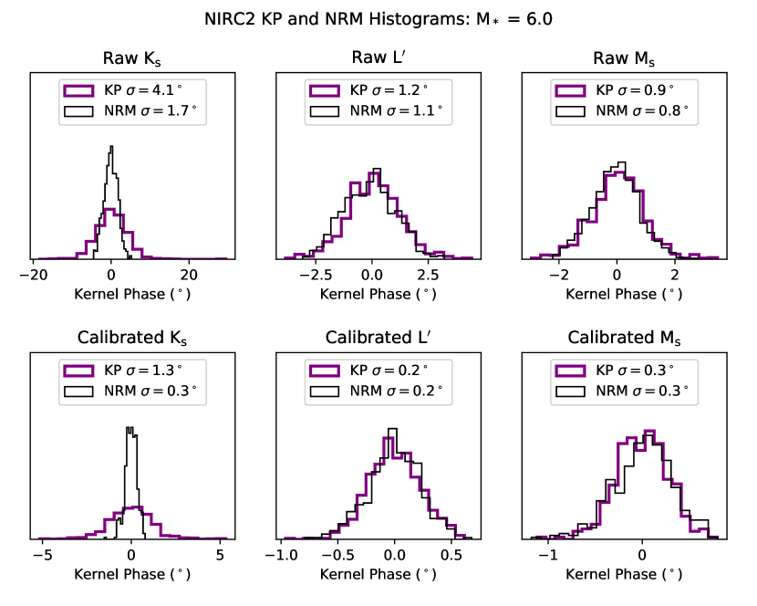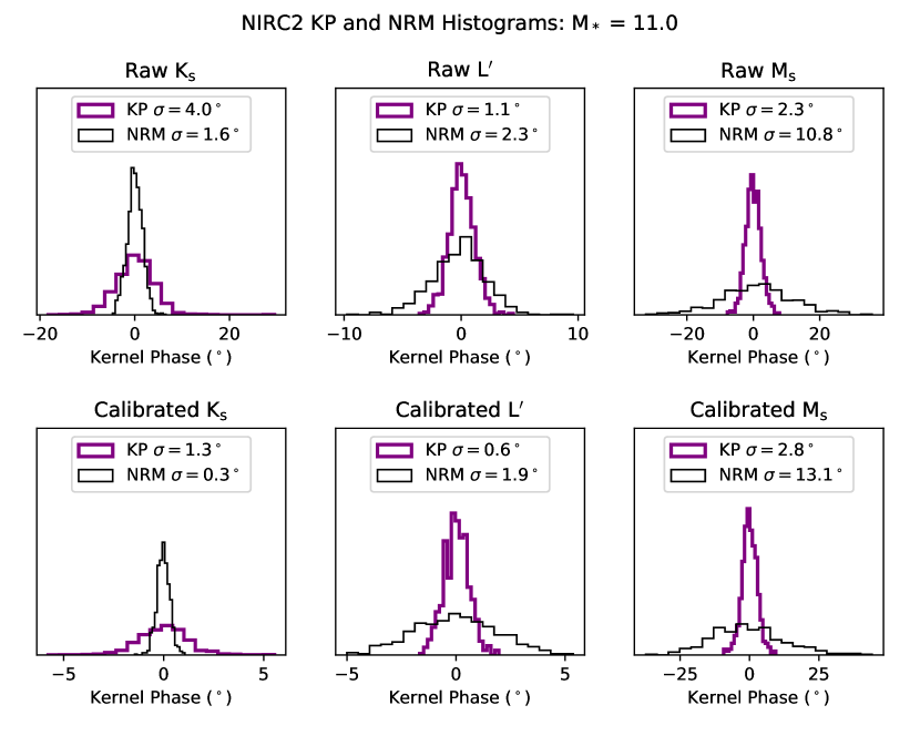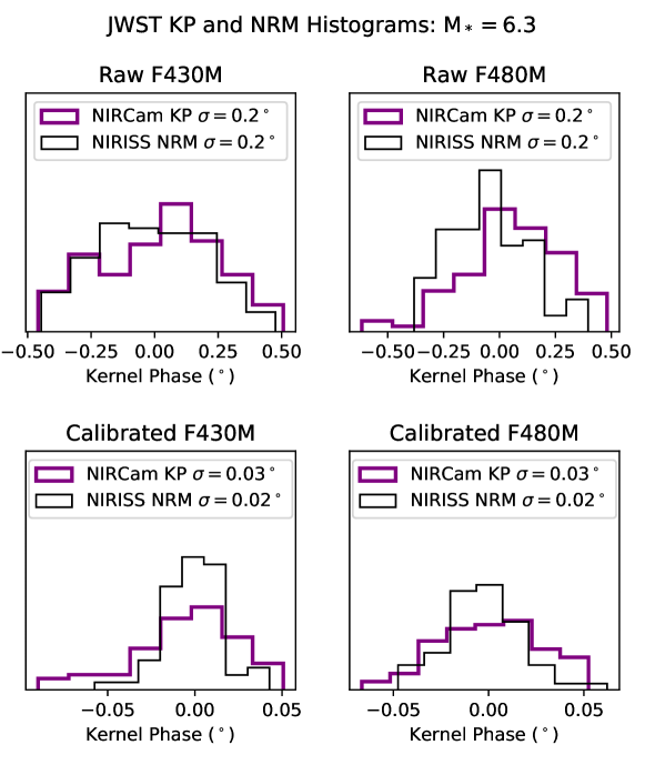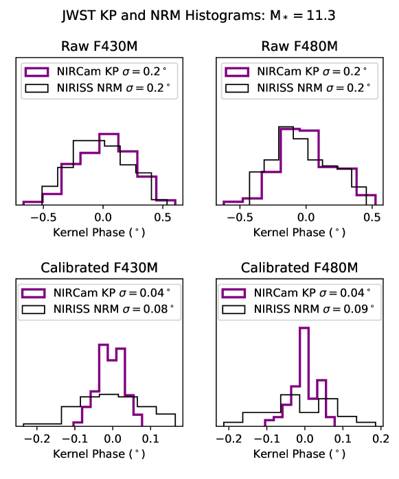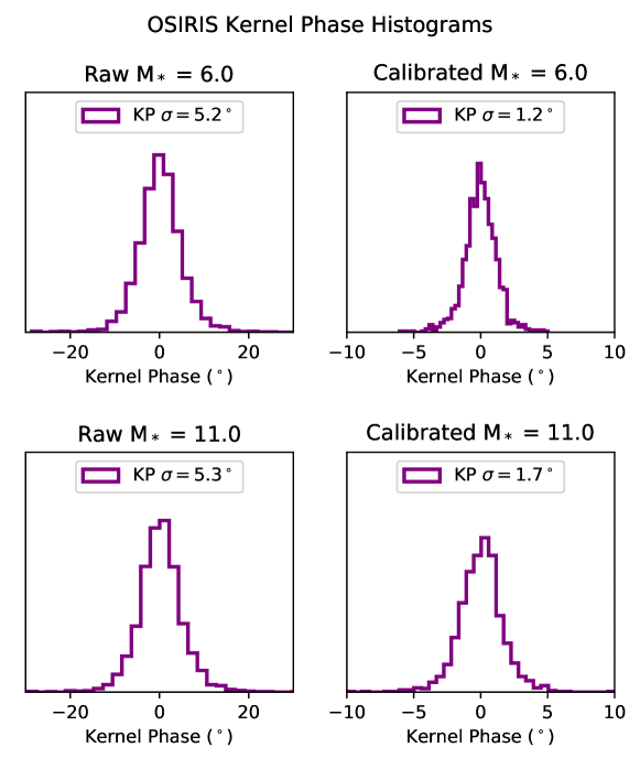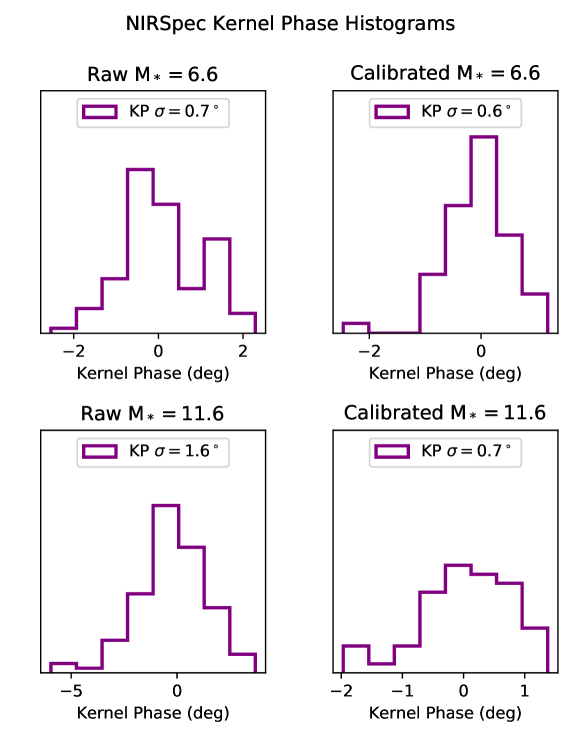Appendix D Scaling Contrast Curves for Other Target Stars and Observing Parameters

Since we provided contrasts for a small range of target star brightnesses, here we discuss how to adapt them to other target stars and observing scenarios. If the amount of observing time per visit and number of visits is kept fixed, and the target star magnitude is decreased below an absolute magnitude of 6, for all observing modes presented here one would expect a similar contrast to the $\mathrm{M_{*}=6}$ case. This is because the $\mathrm{M_{*}=6}$ observations represent the contrast limit, where OPD and calibration errors dominate. However, for all target star brightnesses, increasing the number of (assumed independent) visits would increase the achievable contrast in the bright limit by a factor of $\sqrt{\mathrm{N_{visits,new}}/\mathrm{N_{visits,old}}}$.

For the stars that are not contrast limited - e.g. for observing stars that are fainter than $\mathrm{M_{*}=11-12}$ - if the observing time and number of visits were kept fixed, the contrast would decrease as the target star magnitude increased. Since the kernel phase signal to noise is proportional to $\sqrt{\mathrm{N_{photons,target}}}$, the contrast would scale as $\sqrt{\mathrm{flux_{target,new}}}/\sqrt{\mathrm{flux_{target,old}}}$. However the kernel phase scatter is also proportional to the square root of the number of sky background photons $\sqrt{\mathrm{N_{photons,sky}}}$; for high enough target star magnitudes eventually the background noise would dominate the kernel phases completely. This is already apparent in the upper regions of the $\mathrm{M_{s}}$ NRM and kernel phase panels in Figure 11. If one were to scale the observing time per visit for stars not in the contrast limit, the contrast would increase as $\sqrt{\mathrm{t_{visit,new}/t_{visit,old}}}$, until the contrast limit is reached.