Structured space-sphere point processes and $K$-functions

Abstract

This paper concerns space-sphere point processes, that is, point processes on the product space of $\mathbb{R}^{d}$ (the $d$-dimensional Euclidean space) and $\mathbb{S}^{k}$ (the $k$-dimensional sphere). We consider specific classes of models for space-sphere point processes, which are adaptations of existing models for either spherical or spatial point processes. For model checking or fitting, we present the space-sphere $K$-function which is a natural extension of the inhomogeneous $K$-function for point processes on $\mathbb{R}^{d}$ to the case of space-sphere point processes. Under the assumption that the intensity and pair correlation function both have a certain separable structure, the space-sphere $K$-function is shown to be proportional to the product of the inhomogeneous spatial and spherical $K$-functions. For the presented space-sphere point process models, we discuss cases where such a separable structure can be obtained. The usefulness of the space-sphere $K$-function is illustrated for real and simulated datasets with varying dimensions $d$ and $k$.

First and second order separability, functional summary statistic, log Gaussian Cox process, pair correlation function, shot noise Cox process.

1 Introduction

Occasionally point processes arise on more complicated spaces than the usual space $\mathbb{R}^{d}$, the $d$-dimensional Euclidean space, as for spatio-temporal point processes, spherical point processes or point processes on networks (see Dvořák and Prokešová, 2016; Lawrence et al., 2016; Møller and Rubak, 2016; Baddeley et al., 2017, and the references therein for details on such point processes). In this paper we consider space-sphere point processes that live on the product space $S=\mathbb{R}^{d}\times\mathbb{S}^{k}$, where $\mathbb{S}^{k}=\{u\in\mathbb{R}^{k+1}:\|u\|_{k+1}=1\}$ is the $k$-dimensional unit sphere, $\|\cdot\|_{k}$ denotes the usual distance in $\mathbb{R}^{k}$, and $d,k\in\{1,2,\ldots\}$. For each point $(y,u)\in S$ belonging to a given space-sphere point process, we call $y$ its spatial component and $u$ its spherical component. Assuming local finiteness of a space-sphere point process, the spatial components constitute a locally finite point process in $\mathbb{R}^{d}$, but the spherical components do not necessarily form a finite point process on $\mathbb{S}^{k}$. However, in practice the spatial components are only considered within a bounded window $W\subset\mathbb{R}^{d}$, and the associated spherical components do constitute a finite point process.

One example is the data shown in Figure 1 that consists of the location and orientation of a number of pyramidal neurons found in a small area of a healthy human’s primary motor cortex. More precisely, the locations are three-dimensional coordinates each describing the placement of a pyramidal neuron’s nucleolus, and the orientations are unit vectors pointing from a neuron’s nucleolus toward its apical dendrite. These data can be considered as a realisation of a space-sphere point process with dimensions $d=3$ and $k=2$, where the spatial components describe the nucleolus locations and the spherical components are the orientations. How neurons (of which around $75\text{\,}\%80\text{\,}\%$ are pyramidal neurons) are arranged have been widely discussed in the literature. Specifically, it is hypothesised that neurons are arranged in columns perpendicular to the pial surface of the brain. This hypothesis, referred to as the minicolumn hypothesis, have been studied for more than half a century (see e.g. Lorente de Nó, 1938; Mountcastle, 1978; Buxhoeveden and Casanova, 2002), and it is believed that deviation from such a columnar structure is linked with neurological diseases such as Alzheimers and schizophrenia.

Another example is the time and geographic location of fireballs, which are bright meteors reaching a visual magnitude of $-3$ or brighter. They are continually recorded by U.S. Government sensors and made available at http://neo.jpl.nasa.gov/fireballs/. We can consider fireball events as a space-sphere point process with dimensions $d=1$ and $k=2$, where the time and locations are the spatial and spherical components, respectively. Figure 2 shows the location of fireballs on the globe (identified with the unit sphere) observed over a time period of about 606 weeks.

The paper is organised as follows. In Section 2, we define concepts related to space-sphere point processes and give some natural examples of such processes. In Section 3, we define the space-sphere $K$-function, a functional summary statistic which is analogue to the space-time $K$-function when $d=2$ and $\mathbb{S}^{k}$ is replaced by the time axis (Diggle et al., 1995; Gabriel and Diggle, 2009; Møller and Ghorbani, 2012). The space-sphere $K$-function is defined in terms of the pair correlation function which is assumed to have a certain stationary form. In the case where both the intensity and pair correlation function have a specific separable structure discussed in Section  4, the space-sphere $K$-function is shown to be proportional to the product of the spatial $K$-function (Baddeley et al., 2000) and the spherical $K$-function (Lawrence et al., 2016; Møller and Rubak, 2016). Further, an unbiased estimate is given in Section 5. In Section 6, the usefulness of the space-sphere $K$-function is illustrated for the fireball and neuron data as well as for simulated data, and it is e.g. seen how the $K$-function may be used to test for independence between the spatial and spherical components.

Figure 1: Location and orientation of pyramidal neurons in a small section of a human brain. For details, see Section 6.2.

Figure 2: Top: orthographic projection of the fireball locations. Bottom: time of fireball events measured in weeks. For details, see Section 6.1.

2 Preliminaries

2.1 Setting

Throughout this paper we consider the following setting.

Equip $\mathbb{R}^{d}$ with the Lebesgue measure $|A|=\int_{A}\,\mathrm{d}y$ and $\mathbb{S}^{k}$ with Lebesgue/surface measure $\nu(B)$, where $A\subseteq\mathbb{R}^{d}$ and $B\subseteq\mathbb{S}^{k}$ are Borel sets. Thus, the product space $S=\mathbb{R}^{d}\times\mathbb{S}^{k}$ is equipped with Lebesgue measure $\mu$ given by $\mu(A\times B)=|A|\nu(B)$.

Let $X$ be a simple locally finite point process on $S$, that is, we can view $X$ as a random subset of $S$ such that the restriction $X_{B}=X\cap B$ of $X$ to any bounded set $B\subset S$ is finite. We call $X$ a space-sphere point process, and assume that it has intensity function $\rho$ with respect to $\mu$ and pair correlation function $g$ with respect to the product measure $\mu\otimes\mu$. That is, for any Borel function $h:S\mapsto[0,\infty)$,

$$\mathrm{E}\Bigl{\{}\sum_{(y_{i},u_{i})\in X}h(y_{i},u_{i})\Bigr{\}}=\int h(y,u)\rho(y,u)\,\mathrm{d}\mu(y,u),$$ (2.1)

provided this integral is finite. We say that $X$ is (first order) homogeneous if $\rho$ is a constant function. Furthermore, for any Borel function $k:S\times S\mapsto[0,\infty)$,

$$\mathrm{E} \Bigl{\{}\sum^{\neq}_{(y_{i},u_{i}),(y_{j},u_{j})\in X}k(y_{i},u_{i},y_{j},u_{j})\Bigr{\}}$$ (2.2)

$$=\iint k(y_{1},u_{1},y_{2},u_{2})\rho(y_{1},u_{1})\rho(y_{2},u_{2})g(y_{1},u_{1},y_{2},u_{2})\,\mathrm{d}\mu(y_{1},u_{1})\,\mathrm{d}\mu(y_{2},u_{2}),$$

provided this double integral is finite. Here, we set $g(y_{1},u_{1},y_{2},u_{2})=0$ if $\rho(y_{1},u_{1})\cdot\rho(y_{2},u_{2})=0$, and $\sum^{\neq}_{(y_{i},u_{i}),(y_{j},u_{j})\in X}$ means that we sum over pairs of distinct points $(y_{i},u_{i}),(y_{j},u_{j})\in X$.

The functions $\rho$ and $g$ are unique except for null sets with respect to $\mu$ and $\mu\otimes\mu$, respectively. For ease of presentation, we ignore null sets in the following. Note that $g(y_{1},u_{1},y_{2},u_{2})=g(y_{2},u_{2},y_{1},u_{1})$ is symmetric on $S\times S$. We say that $X$ is stationary in space if its distribution is invariant under translations of its spatial components; this implies that $\rho(y,u)$ depends only on $u$, and $g(y_{1},u_{1},y_{2},u_{2})$ depends only on $(y_{1},y_{2})$ through the difference $y_{1}-y_{2}$. If the distribution of $X$ is invariant under rotations (about the origin in $\mathbb{R}^{d}$) of its spatial components, we say that $X$ is isotropic in space. Stationarity and isotropy in space imply that $g(y_{1},u_{1},y_{2},u_{2})$ depends only on $(y_{1},y_{2})$ through the distance $\|y_{1}-y_{2}\|_{d}$. We say that $X$ is isotropic on the sphere if its distribution is invariant under rotations (on $\mathbb{S}^{k}$) of its spherical components; this implies that $g(y_{1},u_{1},y_{2},u_{2})$ depends only on $(u_{1},u_{2})$ through the geodesic (great circle/shortest path) distance $d(u_{1},u_{2})$ on $\mathbb{S}^{k}$. If $X$ is stationary in space and isotropic on the sphere, then $\rho$ is constant and

$$g(y_{1},u_{1},y_{2},u_{2})=g_{0}\{y_{1}-y_{2},d(u_{1},u_{2})\},\qquad y_{1},y_{2}\in\mathbb{R}^{d},\ u_{1},u_{2}\in\mathbb{S}^{k},$$ (2.3)

depends only on $(y_{1},y_{2})$ through $y_{1}-y_{2}$ and on $(u_{1},u_{2})$ through $d(u_{1},u_{2})$ (this property is studied further in Section 3). If it is furthermore assumed that $X$ is isotropic in space, then

$$g(y_{1},u_{1},y_{2},u_{2})=g_{*}\{\|y_{1}-y_{2}\|_{d},d(u_{1},u_{2})\},\qquad y_{1},y_{2}\in\mathbb{R}^{d},\ u_{1},u_{2}\in\mathbb{S}^{k},$$

depends only on $(y_{1},y_{2})$ through $\|y_{1}-y_{2}\|_{d}$ and on $(u_{1},u_{2})$ through $d(u_{1},u_{2})$.

The spatial components of $X$ constitute a usual spatial point process $Y=\{y:(y,u)\in X\}$, which is locally finite, whereas the spherical components constitute a point process on the sphere $U=\{u:(y,u)\in X\}$ that may be infinite on the compact set $\mathbb{S}^{k}$. Let $W\subset\mathbb{R}^{d}$ be a bounded Borel set, which we may think of as a window where the spatial components $Y_{W}=Y\cap W$ are observed. As $X$ is locally finite, the spherical components associated with $Y_{W}$ constitute a finite point process $U_{W}=\{u:(y,u)\in X,y\in W\}$ on $\mathbb{S}^{k}$. Let $N=N(W)$ denote the cardinality of $Y_{W}$. To avoid trivial and undesirable cases, we assume that $|W|>0$ and that the following inequalities hold:

$$0<\mathrm{E}(N)<\infty$$ (2.4)

and

$$0<\mathrm{E}\{N(N-1)\}<\infty,$$ (2.5)

where, by (2.1)–(2.2),

$$\mathrm{E}(N)=\int_{W\times\mathbb{S}^{k}}\rho(y,u)\,\mathrm{d}\mu(y,u)$$

and

$$\mathrm{E}\{N(N-1)\}$$

$$=\int_{W\times\mathbb{S}^{k}}\int_{W\times\mathbb{S}^{k}}\rho(y_{1},u_{1})\rho(y_{2},u_{2})g(y_{1},u_{1},y_{2},u_{2})\,\mathrm{d}\mu(y_{1},u_{1})\,\mathrm{d}\mu(y_{2},u_{2}).$$

Note that $Y$ has intensity function $\rho_{1}$ and pair correlation function $g_{1}$ given by

$$\rho_{1}(y)=\int\rho(y,u)\,\mathrm{d}\nu(u),\qquad y\in\mathbb{R}^{d},$$ (2.6)

and

$$\rho_{1}(y_{1})\rho_{1}(y_{2})g_{1}(y_{1},y_{2})=\iint\rho(y_{1},u_{1})\rho(y_{2},u_{2})g(y_{1},u_{1},y_{2},u_{2})\,\mathrm{d}\nu(u_{1})\,\mathrm{d}\nu(u_{2})$$ (2.7)

for $y_{1},y_{2}\in\mathbb{R}^{d}$, where we set $g_{1}(y_{1},y_{2})=0$ if $\rho_{1}(y_{1})\rho_{1}(y_{2})=0$. This follows from (2.1)–(2.2) and definitions of the intensity and pair correlation function for spatial point processes (see e.g. Møller and Waagepetersen, 2004). Clearly, if $X$ is stationary in space, then $Y$ is stationary, $\rho_{1}$ is constant, and $g_{1}(y_{1},y_{2})$ is stationary, that is, it depends only on $y_{1}-y_{2}$. If in addition $X$ is isotropic in space, then $g_{1}(y_{1},y_{2})$ is isotropic, that is, it depends only on $\|y_{1}-y_{2}\|_{d}$. On the other hand if $Y$ is stationary (or isotropic) and the spherical components are independent of $Y$, then $X$ is stationary (or isotropic) in space.

Similarly, using definitions of the intensity and pair correlation function for point processes on the sphere (Lawrence et al., 2016; Møller and Rubak, 2016), $U_{W}$ has intensity function $\rho_{2}$ (with respect to $\nu$) and pair correlation function $g_{2}$ (with respect to $\nu\otimes\nu$) given by

$$\rho_{2}(u)=\int_{W}\rho(y,u)\,\mathrm{d}y,\qquad u\in\mathbb{S}^{k},$$ (2.8)

and

$$\rho_{2}(u_{1})\rho_{2}(u_{2})g_{2}(u_{1},u_{2})=\int_{W}\int_{W}\rho(y_{1},u_{1})\rho(y_{2},u_{2})g(y_{1},u_{1},y_{2},u_{2})\,\mathrm{d}y_{1}\,\mathrm{d}y_{2}$$ (2.9)

for $u_{1},u_{2}\in\mathbb{S}^{k}$, where we set $g_{2}(u_{1},u_{2})=0$ if $\rho_{2}(u_{1})\rho_{2}(u_{2})=0$. Note that we suppress in the notation that $\rho_{2}$ and $g_{2}$ depend on $W$. Obviously, if $X$ is isotropic on the sphere, then $\rho_{2}$ is constant and $g_{2}(u_{1},u_{2})$ is isotropic as it depends only on $d(u_{1},u_{2})$.

2.2 Examples

The following examples introduce the point process models considered in this paper.

Example 1 (Poisson and Cox processes).

First, suppose $X$ is a Poisson process with a locally integrable intensity function $\rho$. This means that, the count $N(A)=\#X_{A}$ is Poisson distributed with mean $\int_{A}\rho(y,u)\,\mathrm{d}\mu(y,u)$ for any bounded Borel set $A\subset S$ and, conditional on $N(A)$, the points in $X_{A}$ are independent and identically distributed (IID) with a density proportional to $\rho$ restricted to $A$. Note that $g=1$. Further, $X$ is stationary in space and isotropic on the sphere if and only if $\rho$ is constant, in which case we call $X$ a homogeneous Poisson process with intensity $\rho$. Furthermore, $Y$ and $U_{W}$ are Poisson processes, so $g_{1}=1$ and $g_{2}=1$.

Second, let $\Lambda=\{\Lambda(y,u):(y,u)\in S\}$ be a non-negative random field so that with probability one $\int_{A}\Lambda(y,u)\,\mathrm{d}\mu(y,u)$ is finite for any bounded Borel set $A\subset S$. If $X$ conditioned on $\Lambda$ is a Poisson process with intensity function $\Lambda$, then $X$ is said to be a Cox process driven by $\Lambda$ (Cox, 1955). Clearly, the intensity and pair correlation functions of $X$ are

$$\rho(y,u)=\mathrm{E}\{\Lambda(y,u)\},\qquad y\in\mathbb{R}^{d},\ u\in\mathbb{S}^{k},$$ (2.10)

and

$$\rho(y_{1},u_{1})\rho(y_{2},u_{2})g(y_{1},u_{1},y_{2},u_{2})=\mathrm{E}\{\Lambda(y_{1},u_{1})\Lambda(y_{2},u_{2})\},$$

for $y_{1},y_{2}\in\mathbb{R}^{d},\ u_{1},u_{2}\in\mathbb{S}^{k}$. To separate the intensity function $\rho$ from random effects, it is convenient to work with a so-called residual random field $R=\{R(y,u):(y,u)\in S\}$ fulfilling $\Lambda(y,u)=\rho(y,u)R(y,u)$, so $\mathrm{E}\{R(y,u)\}=1$ (see e.g. Møller and Waagepetersen, 2007; Diggle, 2014). Then

$$g(y_{1},u_{1},y_{2},u_{2})=\mathrm{E}\{R(y_{1},u_{1})R(y_{2},u_{2})\},\qquad y_{1},y_{2}\in\mathbb{R}^{d},\ u_{1},u_{2}\in\mathbb{S}^{k},$$ (2.11)

$\mbox{whenever }\rho(y_{1},u_{1})\rho(y_{2},u_{2})>0$.

Note that projected point processes $Y$ and $U_{W}$ are Cox processes driven by the random fields $\{\int_{\mathbb{S}^{k}}\Lambda(y,u)\,\mathrm{d}\nu(u):y\in\mathbb{R}^{d}\}$ and $\{\int_{W}\Lambda(y,u)\,\mathrm{d}y:u\in\mathbb{S}^{k}\}$, respectively. Their intensity and pair correlation functions are specified by (2.6)–(2.9).

Example 2 (Log Gaussian Cox processes).

A Cox process $X$ is called a log Gaussian Cox process (LGCP; Møller et al., 1998) if the residual random field is of the form $R=\exp(Z)$, where $Z$ is a Gaussian random field (GRF) with mean function $\mu(y,u)=-c(y,u,y,u)/2$, where $c$ is the covariance function of $Z$. Note that $X$ has pair correlation function

$$g(y_{1},u_{1},y_{2},u_{2})=\exp\left[c\{(y_{1},u_{1}),(y_{2},u_{2})\}\right],\qquad y_{1},y_{2}\in\mathbb{R}^{d},\,u_{1},u_{2}\in\mathbb{S}^{k}.$$ (2.12)

Example 3 (Marked point processes).

It is sometimes useful to view $X$ as a marked point process (see e.g. Daley and Vere-Jones, 2003; Illian et al., 2008), where the spatial components are treated as the ground process and the spherical components as marks. Often it is of interest to test the hypothesis $H_{0}$ that the marks are IID and independent of the ground process $Y$. Under $H_{0}$, with each mark following a density $p$ with respect to $\nu$, the intensity is

$$\rho(y,u)=\rho_{1}(y)p(u),\qquad y\in\mathbb{R}^{d},\,u\in\mathbb{S}^{k},$$

and the pair correlation function

$$g(y_{1},u_{1},y_{2},u_{2})=g_{1}(y_{1},y_{2}),\qquad y_{1},y_{2}\in\mathbb{R}^{d},\,u_{1},u_{2}\in\mathbb{S}^{k},$$

does not depend on $(u_{1},u_{2})$.

In some situations, it may be more natural to look at it conversely, that is, treating $U_{W}$ as the ground process and $Y_{W}$ as marks. Then similar results for $\rho$ and $g$ may be established by interchanging the roles of points and marks.

Example 4 (Independently marked determinantal point processes).

Considering a space-sphere point process $X$ as a marked point process that fulfils the hypothesis $H_{0}$ given in Example 3, we may let the ground process $Y$ be distributed according to any point process model of our choice regardless of the marks $U$. For instance, in case of repulsion between the points in $Y$, a determinantal point process (DPP) may be of interest because of its attractive properties (see Lavancier et al., 2015, and the references therein). Briefly, a DPP is defined by a so-called kernel $C:\mathbb{R}^{d}\times\mathbb{R}^{d}\to\mathbb{C}$, which we assume is a complex covariance function, that is, $C$ is positive semi-definite and Hermitian. Furthermore, let $\rho_{1}^{(n)}$ denote the $n$th order joint intensity function of $Y$, that is, $\rho_{1}^{\smash{(}1\smash{)}}=\rho_{1}$ is the intensity and $\rho_{1}^{\smash{(}2\smash{)}}(y_{1},y_{2})=\rho_{1}(y_{1})\rho_{1}(y_{2})g_{1}(y_{1},y_{2})$ for $y_{1},y_{2}\in\mathbb{R}^{d}$, while we refer to Lavancier et al. (2015) for the general definition of $\rho_{1}^{\smash{(}n\smash{)}}$ which is an extension of (2.6)–(2.7). If for all $n=1,2,\dots$,

$$\rho_{1}^{\smash{(}n\smash{)}}(y_{1},\dots,y_{n})=\det\{C(y_{i},y_{j})\}_{i,j=1,\dots,n},\qquad y_{1},\dots,y_{n}\in\mathbb{R}^{d},$$

where $\det\{C(y_{i},y_{j})\}_{i,j=1,\dots,n}$ is the determinant of the $n\times n$ matrix with $(i,j)$-entry $C(y_{i},y_{j})$, we call $Y$ a DPP with kernel $C$ and refer to $X$ as an independently marked DPP. It follows that $Y$ has intensity function $\rho(y)=C(y,y)$ and pair correlation function

$$g_{1}(y_{1},y_{2})=1-|R(y_{1},y_{2})|^{2},\qquad y_{1},y_{2}\in\mathbb{R}^{d},$$

whenever $\rho(y_{1})\rho(y_{2})>0$, where $R(y_{1},y_{2})=C(y_{1},y_{2})/\sqrt{C(y_{1},y_{1})C(y_{2},y_{2})}$ is the correlation function corresponding to $C$ and $|z|$ denotes the modulus of $z\in\mathbb{C}$.

Alternatively, we may look at a DPP on the sphere (Møller et al., 2018), that is, modelling $U_{W}$ as a DPP while considering $Y_{W}$ as the marks and impose the conditions of IID marks independent of $U_{W}$.

3 The space-sphere $K$-function

3.1 Definition

When (2.3) holds we say that the space-sphere point process $X$ is second order intensity-reweighted stationary (SOIRS) and define the space-sphere $K$-function by

$$K(r,s)=\int_{\|y\|_{d}\leq r,\,d(u,e)\leq s}g_{0}\{y,d(u,e)\}\,\mathrm{d}\mu(y,u),\qquad r\geq 0,\,0\leq s\leq\pi,$$ (3.1)

where $e\in\mathbb{S}^{k}$ is an arbitrary reference direction. This definition does not depend on the choice of $e$, as the integrand only depends on $u\in\mathbb{S}^{k}$ through its geodesic distance to $e$ and $\nu(\cdot)$ is a rotation invariant measure. For example, we may let $e=(0,\ldots,0,1)\in\mathbb{S}^{k}$ be the “North Pole”.

Let $\sigma_{k}=\nu(\mathbb{S}^{k})=2\pi^{(k+1)/2}/\Gamma\{(k+1)/2\}$ denote the surface measure of $\mathbb{S}^{k}$. For any Borel set $B\subset\mathbb{R}^{d}$ with $0<|B|<\infty$, we easily obtain from (2.2) and (3.1) that

$$K(r,s)$$

$$=\frac{1}{|B|\sigma_{k}}\iint_{y_{1}\in B,\,\|y_{1}-y_{2}\|_{d}\leq r,\,d(u_{1},u_{2})\leq s}g_{0}\{y_{1}-y_{2},d(u_{1},u_{2})\}\,\mathrm{d}\mu(y_{1},u_{1})\,\mathrm{d}\mu(y_{2},u_{2})$$

$$=\frac{1}{|B|\sigma_{k}}\mathrm{E}\Bigl{[}\sum^{\neq}_{(y_{i},u_{i}),(y_{j},u_{j})\in X}\frac{\mathbb{I}\{y_{i}\in B,\,\|y_{i}-y_{j}\|_{d}\leq r,\,d(u_{i},u_{j})\leq s\}}{\rho(y_{i},u_{i})\rho(y_{j},u_{j})}\Bigr{]}$$ (3.2)

for $r\geq 0,\,0\leq s\leq\pi$, where $\mathbb{I}(\cdot)$ denotes the indicator function. The relation given by (3.2) along with the requirement that the expression in (3.2) does not depend on the choice of $B$ could alternatively have been used as a more general definition of the space-sphere $K$-function. Such a definition is in agreement with the one used in Baddeley et al. (2000) for SOIRS of a spatial point process. It is straightforward to show that (3.2) does not depend on $B$ when $X$ is stationary in space.

For $r,s>0$ and $(y_{1},u_{1}),(y_{2},u_{2})\in S$, we say that $(y_{1},u_{1})$ and $(y_{2},u_{2})$ are $(r,s)$-close neighbours if $\|y_{1}-y_{2}\|_{d}\leq r$ and $d(u_{1},u_{2})\leq s$. If $X$ is stationary in space and isotropic on the sphere, then (3.2) shows that $\rho K(r,s)$ can be interpreted as the expected number of further $(r,s)$-close neighbours in $X$ of a typical point in $X$. More formally, this interpretation relates to the reduced Palm distribution (Daley and Vere-Jones, 2003).

Some literature treating marked point processes discuss the so-called mark-weighted $K$-function (see e.g. Illian et al., 2008; Koubek et al., 2016), which to some extent resembles the space-sphere $K$-function in a marked point process context; both are cumulative second order summary functions that consider points as well as marks. However, the mark-weighted $K$-function has an emphasis on the marked point process setup (and considers e.g. $\rho_{1}$ rather than $\rho$), whereas the space-sphere $K$-function is constructed in such a way that it is an analogue to the planar/spherical $K$-function for space-sphere point processes.

0 Example 1 continued (Poisson and Cox processes).

A Poisson process is clearly SOIRS and $K(r,s)$ is simply the product of the volume of a $d$-dimensional ball with radius $r$ and the surface area of a spherical cap given by $\{u\in\mathbb{S}^{k}:d(u,e)\leq s\}$ for an arbitrary $e\in\mathbb{S}^{k}$ (see Li, 2011, for formulas of this area). Thus, for $r\geq 0$, the space-sphere $K$-function is

$$K_{Pois}(r,s)=\begin{cases}\frac{r^{d}\pi^{(d+k+1)/2}}{\Gamma(1+d/2)\Gamma\{(k+1)/2\}}I_{\sin^{2}(s)}\left(\frac{k}{2},\frac{1}{2}\right),\qquad 0\leq s\leq\frac{\pi}{2},\\[5.0pt] \frac{r^{d}\pi^{(d+k+1)/2}}{\Gamma(1+d/2)\Gamma\{(k+1)/2\}}\{2-I_{\sin^{2}(\pi-s)}(\frac{k}{2},\frac{1}{2})\},\qquad\frac{\pi}{2}<s\leq\pi,\end{cases}$$

where $I_{x}(a,b)$ is the regularized incomplete beta function. In particular, if $k=2$,

$$\begin{rcases}I_{\sin^{2}(s)}(\frac{k}{2},\frac{1}{2}),&0\leq s\leq\frac{\pi}{2}\\ 2-I_{\sin^{2}(\pi-s)}(\frac{k}{2},\frac{1}{2}),&\frac{\pi}{2}<s\leq\pi\end{rcases}=1-\cos(s).$$

If the residual random field $R$ in (2.11) is invariant under translations in $\mathbb{R}^{d}$ and under rotations on $\mathbb{S}^{k}$, then the associated Cox process is SOIRS. The evaluation of $g$ (and thus $K$) depends on the particular model of $R$ as exemplified in Example 2 below and in Section 7.

0 Example 2 continued (LGCPs).

Suppose that the distribution of $R$ is invariant under translations in $\mathbb{R}^{d}$ and under rotations on $\mathbb{S}^{k}$, and recall that $R$ is required to have unit mean. Then the underlying GRF $Z$ has a covariance function of the form

$$c(y_{1},u_{1},y_{2},u_{2})=c_{0}\{y_{1}-y_{2},d(u_{1},u_{2})\},\qquad y_{1},y_{2}\in\mathbb{R}^{d},\ u_{1},u_{2}\in\mathbb{S}^{k},$$

and $\mathrm{E}Z(y,u)=-\sigma^{2}/2$ for all $y\in\mathbb{R}^{d}$ and $u\in\mathbb{S}^{k}$, where $\sigma^{2}=c_{0}(0,0)$ is the variance. It then follows from (2.12) that $X$ is SOIRS with

$$g_{0}(y,s)=\exp\{c_{0}(y,s)\},\qquad y\in\mathbb{R}^{d},\ 0\leq s\leq\pi.$$ (3.3)

4 Separability

4.1 First order separability

We call the space-sphere point process $X$ first order separable if there exist non-negative Borel functions $f_{1}$ and $f_{2}$ such that

$$\rho(y,u)=f_{1}(y)f_{2}(u),\qquad y\in\mathbb{R}^{d},\ u\in\mathbb{S}^{k}.$$

By (2.4), (2.6), and (2.8) this is equivalent to

$$\rho(y,u)=\rho_{1}(y)\rho_{2}(u)/{\mathrm{E}(N)},\qquad y\in\mathbb{R}^{d},\ u\in\mathbb{S}^{k},$$ (4.1)

recalling that $\rho_{2}$ and $N$ depend on $W$, but $\rho_{2}/\mathrm{E}N$ does not depend on the choice of $W$. Then, in a marked point process setup where the spherical components are treated as marks, $\rho_{2}(\cdot)/{\mathrm{E}(N)}$ is the density of the mark distribution. First order separability was seen in Example 3 to be fulfilled under the assumption of IID marks independent of the ground process. Moreover, any homogeneous space-sphere point process is clearly first order separable. In practice, first order separability is a working hypothesis which may be hard to check.

4.2 Second order separability

If there exist Borel functions $k_{1}$ and $k_{2}$ such that

$$g(y_{1},u_{1},y_{2},u_{2})=k_{1}(y_{1},y_{2})k_{2}(u_{1},u_{2}),\qquad y_{1},y_{2}\in\mathbb{R}^{d},\ u_{1},u_{2}\in\mathbb{S}^{k},$$

we call $X$ second order separable. Assuming first order separability, it follows by (2.5), (2.7), (2.9), and (4.1) that second order separability is equivalent to

$$g(y_{1},u_{1},y_{2},u_{2})=\beta g_{1}(y_{1},y_{2})g_{2}(u_{1},u_{2}),\qquad y_{1},y_{2}\in\mathbb{R}^{d},\ u_{1},u_{2}\in\mathbb{S}^{k},$$ (4.2)

where

$$\beta={\mathrm{E}(N)^{2}}/{{\mathrm{E}\{N(N-1)\}}}$$

and noting that $\beta$ and $g_{2}$ depend on $W$, but $\beta g_{2}$ does not depend on the choice of $W$. The value of $\beta$ may be of interest: for a Poisson Process, $\beta=1$; for a Cox process, $\mathrm{var}(N)\geq\mathrm{E}(N)$ (see e.g. Møller and Waagepetersen, 2004), so $\beta\leq 1$; for an independently marked DPP, $\beta\geq 1$ (Lavancier et al., 2015).

0 Example 1 continued (Poisson and Cox processes).

Clearly, when $X$ is a Poisson process, it is second order separable. Assume instead that $X$ is a Cox process and the residual random field is separable, that is, $R(y,u)=R_{1}(y)R_{2}(u)$, where $R_{1}=\{R_{1}(y):y\in\mathbb{R}^{d}\}$ and $R_{2}=\{R_{2}(u):u\in\mathbb{S}^{k}\}$ are independent random fields. Then, by (2.11), $X$ is second order separable and

$$g(y_{1},u_{1},y_{2},u_{2})$$

$$=\mathrm{E}\{R_{1}(y_{1})R_{1}(y_{2})\}\mathrm{E}\{R_{2}(u_{1})R_{2}(u_{2})\},\qquad y_{1},y_{2}\in\mathbb{R}^{d},\ u_{1},u_{2}\in\mathbb{S}^{k}.$$

0 Example 2 continued (LGCPs).

If $X$ is a LGCP driven by $\Lambda(y,u)=\rho(y,u)\cdot\exp\{Z(y,u)\}$, second order separability is implied if $Z_{1}=\log R_{1}$ and $Z_{2}=\log R_{2}$ are independent GRFs so that $Z(y,u)=Z_{1}(y)+Z_{2}(u)$. Then, by the imposed invariance properties of the distribution of the residual random field, $Z_{1}$ must be stationary with a stationary covariance function $c_{1}(y_{1},y_{2})=c_{01}(y_{1}-y_{2})$ and mean $-c_{01}(0)/2$, and $Z_{2}$ must be isotropic with an isotropic covariance function $c_{2}(u_{1},u_{2})=c_{02}\{d(u_{1},u_{2})\}$ and mean $-c_{02}(0)/2$. Consequently, in (3.3), $c_{0}(y,s)=c_{01}(y)+c_{02}(s)$ for $y\in\mathbb{R}^{d}$ and $0\leq s\leq\pi$.

0 Example 3 continued (marked point processes).

Consider the space-sphere point process $X$ as a marked point process with marks in $\mathbb{S}^{k}$. As previously seen, first and second order separability is fulfilled under the assumption of IID marks independent of the ground process, but we may in fact work with weaker conditions to ensure the separability properties as follows. Assume that each mark is independent of the ground process $Y$ and the marks are identically distributed following a density function $p$ with respect to $\nu$. Then the first order separability condition (4.1) is satisfied with $\rho_{2}(u)=\mathrm{E}(N)p(u)$ for $u\in\mathbb{S}^{k}$. In addition, assuming the conditional distribution of the marks given $Y$ is such that any pair of marks is independent of $Y$ and follows the same joint density $q(\cdot,\cdot)$ with respect to $\nu\otimes\nu$, it is easily seen that the second order separability condition (4.2) is satisfied with

$$g_{2}(u_{1},u_{2})=\frac{q(u_{1},u_{2})}{\beta p(u_{1})p(u_{2})},\qquad u_{1},u_{2}\in\mathbb{S}^{k},$$

whenever $\rho_{2}(u_{1})\rho_{2}(u_{2})>0$. If we also have pairwise independence between the marks, that is, $q(u_{1},u_{2})=p(u_{1})p(u_{2})$, then the pair correlation function $g(y_{1},u_{1},\allowbreak y_{2},u_{2})=g_{1}(y_{1},y_{2})$ does not depend on $(u_{1},u_{2})$ and $g_{2}(u_{1},u_{2})=1/\beta$ is constant. Note that this implies $g_{2}\leq 1$ for an independently marked DPP, reflecting that even when the marks are drawn independently of $Y$ the behaviour of the points implicitly affects the marks as the number of points is equal to the number of marks.

Again, the roles of points and marks may be switched resulting in statements analogue to those above.

4.3 Assuming both SOIRS and first and second order separability

Suppose that $X$ is both SOIRS and first and second order separable. Then the space-sphere $K$-function can be factorized as follows. Note that $Y$ and $U_{W}$ are SOIRS since there by (2.3), (2.7), (2.9), and (4.1) exist Borel functions $g_{01}$ and $g_{02}$ such that

$$g_{1}(y_{1},y_{2}) =g_{01}(y_{1}-y_{2})$$ (4.3)

$$=\iint\frac{\rho_{2}(u_{1})}{\mathrm{E}(N)}\frac{\rho_{2}(u_{2})}{\mathrm{E}(N)}g_{0}\{y_{1}-y_{2},d(u_{1},u_{2})\}\,\mathrm{d}\nu(u_{1})\,\mathrm{d}\nu(u_{2})$$

for $y_{1},y_{2}\in\mathbb{R}^{d}\mbox{ with }\rho_{1}(y_{1})\rho_{1}(y_{2})>0$, and

$$g_{2}(u_{1},u_{2}) =g_{02}\{d(u_{1},u_{2})\}$$ (4.4)

$$=\int_{W}\int_{W}\frac{\rho_{1}(y_{1})}{\mathrm{E}(N)}\frac{\rho_{1}(y_{2})}{\mathrm{E}(N)}g_{0}\{y_{1}-y_{2},d(u_{1},u_{2})\}\,\mathrm{d}y_{1}\,\mathrm{d}y_{2}$$

for $u_{1},u_{2}\in\mathbb{S}^{k}\mbox{ with }\rho_{2}(u_{1})\rho_{2}(u_{2})>0$. Hence, the inhomogeneous $K$-function for the spatial components in $Y$ (introduced in Baddeley et al., 2000) is

$$K_{1}(r)=\int_{\|y\|_{d}\leq r}g_{01}(y)\,\mathrm{d}y,\qquad r\geq 0,$$

and the inhomogeneous $K$-function for the spherical components in $U_{W}$ (introduced in Lawrence et al., 2016; Møller and Rubak, 2016) is

$$K_{2}(s)=\int_{d(u,e)\leq s}g_{02}\{d(u,e)\}\,\mathrm{d}\nu(u),\qquad 0\leq s\leq\pi,$$

where $e\in\mathbb{S}^{k}$ is arbitrary. Combining (3.1) and (4.2)–(4.4), we obtain

$$K(r,s)=\beta K_{1}(r)K_{2}(s),\qquad r\geq 0,\,0\leq s\leq\pi.$$

Note that, if $X$ is a first order separable Poisson process, then $D(r,s)=K(r,s)-K_{1}(r)K_{2}(s)$ is 0, and an estimate of $D$ may also be used as a functional summary statistic when testing a Poisson hypothesis.

5 Estimation of $K$-functions

In this section, we assume for specificity that the observation window is $W\times\mathbb{S}^{k}$, where $W\subset\mathbb{R}^{d}$ is a bounded Borel set, and a realisation $X_{W\times\mathbb{S}^{k}}=x_{W\times\mathbb{S}^{k}}$ is observed; in Section 7, we discuss other cases of observation windows. We let $Y_{W}=y_{W}$ and $U_{W}=u_{W}$ be the corresponding sets of observed spatial and spherical components.

First, assume that $\rho_{1}$ and $\rho_{2}$ are known. Following Baddeley et al. (2000), we estimate $K_{1}$ by

$$\hat{K}_{1}(r)=\sum^{\neq}_{y_{i},y_{j}\in y_{W}}\frac{\mathbb{I}(\|y_{i}-y_{j}\|_{d}\leq r)}{w_{1}(y_{i},y_{j})\rho_{1}(y_{i})\rho_{1}(y_{j})},\qquad r\geq 0,$$ (5.1)

where $w_{1}$ is an edge correction factor on $\mathbb{R}^{d}$. If we let $w_{1}(y_{i},y_{j})=|W\cap W_{y_{i}-y_{j}}|$ be the translation correction factor (Ohser, 1983), where $W_{y}=\{y+z:z\in W\}$ denotes the translation of $W$ by $y\in\mathbb{R}^{d}$, then $\hat{K}_{1}$ is an unbiased estimate of $K_{1}$ (see e.g. Lemma 4.2 in Møller and Waagepetersen, 2004). For $d=1$, we may instead use the temporal edge correction factor with $w_{1}(y_{i},y_{j})=|W|$ if $[y_{i}-y_{j},y_{i}+y_{j}]\subseteq W$ and $w_{1}(y_{i},y_{j})=|W|/2$ otherwise (Diggle et al., 1995; Møller and Ghorbani, 2012). Moreover, for estimation of $K_{2}$, we use the unbiased estimate

$$\hat{K}_{2}(s)=\frac{1}{\sigma_{k}}\sum^{\neq}_{u_{i},u_{j}\in u_{W}}\frac{\mathbb{I}\{d(u_{i},u_{j})\leq s\}}{\rho_{2}(u_{i})\rho_{2}(u_{j})},\qquad 0\leq s\leq\pi,$$ (5.2)

cf. Lawrence et al. (2016) and Møller and Rubak (2016). A natural extension of the above estimates gives the following estimate of $K$:

$$\hat{K}(r,s)=\frac{1}{\sigma_{k}}\sum^{\neq}_{(y_{i},u_{i}),(y_{j},u_{j})\in x_{W\times\mathbb{S}^{k}}}\frac{\mathbb{I}\{\|y_{i}-y_{j}\|_{d}\leq r,\,d(u_{i},u_{j})\leq s\}}{w_{1}(y_{i},y_{j})\rho(y_{i},u_{i})\rho(y_{j},u_{j})}$$ (5.3)

for $r\geq 0,\,0\leq s\leq\pi$. This is straightforwardly seen to be an unbiased estimate when $w_{1}$ is the translation correction factor.

Second, in practice we need to replace $\rho_{1}$ in (5.1), $\rho_{2}$ in (5.2), and $\rho$ in (5.3) by estimates, as exemplified in Section 6. This may introduce a bias.

6 Data examples

6.1 Fireball locations over time

Figure 2 shows the time and location of $n=344$ fireballs observed over a time period from 2005-01-01 03:44:09 to 2016-08-12 23:59:59 corresponding to a time frame $W$ of about 606 weeks. The data can be recovered at http://neo.jpl.nasa.gov/fireballs/ using these time stamps. Figure 2 reveals no inhomogeneity of neither fireball locations or event times. Therefore we assumed first order homogeneity, and used the following unbiased estimates for the intensities:

$$\hat{\rho}_{1}=n/|W|=0.57,\ \hat{\rho}_{2}=n/(4\pi)=27.37,\ \hat{\rho}=n/(4\pi|W|)=0.05.$$

Then $\hat{K}_{1}$, $\hat{K}_{2}$, and $\hat{K}$ (with $w_{1}$ in (5.1) and (5.3) equal to the temporal edge correction factor) were used as test functions in three different global rank envelope tests for testing whether fireball event times, locations, and locations over time each could be described by a homogeneous Poisson model with estimated intensity $\hat{\rho}_{1}$, $\hat{\rho}_{2}$, and $\hat{\rho}$, respectively. Appendix A provides a brief account on global rank envelope tests; see also Myllymäki et al. (2017). Under each of the three fitted Poisson processes and using 2499 simulations (as recommended in Myllymäki et al., 2017), we obtained $p$-intervals of $(0.028,0.040)$ for the event times, $(0.908,0.908)$ for the locations, and $(0.445,0.516)$ for the locations over time. The associated $95\%$ global rank envelopes for $\hat{K}_{1}$ and $\hat{K}_{2}$ are shown in Figure 3, and the difference between $\hat{K}$ and the upper and lower $95\%$ global rank envelope is shown in Figure 4. Since $\hat{K}_{2}$ and $\hat{K}$ stay inside the $95\%$ global rank envelopes for the considered distances on $\mathbb{S}^{k}$ and $\mathbb{R}\times\mathbb{S}^{k}$, there is no evidence against a homogeneous Poisson model for neither locations or locations over time. On the other hand, with a conservative $p$-value of $4\%$, the global rank envelope test based on $\hat{K}_{1}$ indicates that a homogeneous Poisson model for the event times is not appropriate. However, the observed test function $\hat{K}_{1}(r)$ falls only outside the envelope in Figure 3 for large values of $r$. Thus, choosing a slightly smaller interval of $r$-values would lead to a different conclusion.

As an alternative to the space-sphere $K$-function, we considered the summary function $D(r,s)$ which in case of a Poisson process is $0$. Estimating $D$ by $\hat{D}(r,s)=\hat{K}(r,s)-\hat{K}_{1}(r)\hat{K}_{2}(s)$, we performed a global rank envelope test with $D$ as test function. The resulting test gave a $p$-interval of $(0.537,0.564)$ which is similar to the one obtained using $\hat{K}$ as test function.

Figure 3: Left: $\hat{K}_{1}(r)-2r$ for the fireball event times (solid curve) along with a 95% global rank envelope (grey area) under a homogeneous Poisson model on the time interval for the observed events. Right: $\hat{K}_{2}(s)-2\pi\{1-\cos(s)\}$ for the fireball locations (solid curve) along with a 95% global rank envelope (grey area) under a homogeneous Poisson model on $\mathbb{S}^{2}$.

Figure 4: Difference between $\hat{K}(r,s)$ for the observed fireball locations over time and the lower ($\hat{K}_{\mathrm{low}}$) or upper ($\hat{K}_{\mathrm{upp}}$) 95% global rank envelope under a homogeneous Poisson model on $W\times\mathbb{S}^{2}$. Left: $\hat{K}(r,s)-\hat{K}_{\mathrm{low}}(r,s)$. Right: $\hat{K}_{\mathrm{upp}}(r,s)-\hat{K}(r,s)$.

6.2 Location and orientation of pyramidal neurons

We now return to the space-sphere point pattern concerning location and orientation of pyramidal neurons described in Section 1, which is a data set collected by Ali H. Rafati, a biomedical and clinical scientist. The point pattern is observed on $W\times\mathbb{S}^{2}$, where $W\subset\mathbb{R}^{3}$ is the rectangular box shown in Figure 1 with side lengths $492.7\text{\,}\mathrm{\SIUnitSymbolMicro m}$, $132.0\text{\,}\mathrm{\SIUnitSymbolMicro m}$, and $407.7\text{\,}\mathrm{\SIUnitSymbolMicro m}$. Due to the way data was collected, 46 neurons in the original dataset had an orientation/unit vector lying exactly in the $x$-$z$ plane, meaning that the orientations of these 46 neurons are located only on a great circle of $\mathbb{S}^{2}$. To keep the analysis simple we disregarded these neurons, resulting in a dataset consisting of $n=504$ neurons. Below we initially discuss an appropriate parametric forms of the intensity for the locations and orientations and how to estimate the intensity parameters. Then we investigate whether the orientations and locations can be described by a Poisson model with the proposed intensity, where we first consider the data as two separate point patterns (a spatial point pattern describing the locations and a spherical point pattern describing the orientations) and next as a space-sphere point pattern.

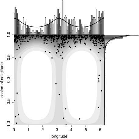
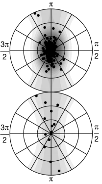
Figure 1 reveals no inhomogeneity for the neuron locations, whereas it is evident that the orientations are inhomogeneous pointing mostly toward the pial surface of the brain (the plane perpendicular to the $z$-axis). Thus, we estimated the intensity of the locations by $\hat{\rho}_{1}=n/|W|=1.9\times 10^{-5}$, and for the orientations we let the intensity be $\rho_{2}(u)=cf(u)$, where $c$ is a positive parameter and $f$ is a density on $\mathbb{S}^{2}$ which we model as follows. Figure 5 indicates that the orientations arise from a mixture of two distributions; one distribution with points falling close to the North Pole and another with points falling in a narrow girdle. Therefore, we let $f(u)=pf_{K}(u)+(1-p)f_{W}(u)$ be the mixture density of a Kent and a Watson distribution on $\mathbb{S}^{2}$ (see e.g. Fisher et al., 1987, for a detailed description of these spherical distributions). In brief, the Kent density, $f_{K}$, depends on five parameters (three directional, one concentration, and one ovalness parameter), and its contours are oval with centre and form specified by the directional parameters. Depending on the values of the ovalness and concentration parameter, the Kent distribution is either uni- or bimodal. Here, to account for the large number of points centred around the North Pole, we consider the unimodal Kent distribution. Furthermore, the Watson density, $f_{W}$, depends on two parameters; a directional parameter determining the centres of the density’s circular contours, and a concentration parameter controlling where and how fast the density peaks. Depending on the sign of the concentration parameter, the density either decreases or increases as the geodesic distance to the centres of the contours increases, giving rise to either a bimodal or girdle shaped distribution. Since the Watson distribution shall describe the orientations on the girdle, the concentration parameter must be negative.

The nine parameters of the proposed intensity function $\rho_{2}$ were estimated as follows. We naturally estimate $c$ by $n$. The orientations occurring on the southern hemisphere are presumed to come from the Watson distribution, while the orientations on the northern hemisphere come from both distributions. Therefore, and because the Watson density on the northern hemisphere is a reflection of the southern hemisphere, we simply estimated the mixture probability by $\hat{p}=1-2n_{s}/n=0.94$, where $n_{s}$ is the observed number of points on the southern hemisphere. The directional parameters were chosen based on expectations expressed by the scientist behind the data collections, which were supported by visual inspection of the data; e.g. the directional parameter for the Kent distribution that determines the centre of the contours was chosen as the North Pole corresponding to the direction perpendicular to the pial surface and consistent with Figure 5. Finally, the concentration and ovalness parameters were estimated by numerical maximization of their likelihood function, giving the estimated density

$$\hat{f}(u)=0.94\,C_{K}\exp\{14.89u_{3}+2.69(u_{1}^{2}-u_{2}^{2})\}+0.06\,C_{W}\exp(-7.88u_{2}^{2}),$$

where $u=(u_{1},u_{2},u_{3})\in\mathbb{S}^{2}$ and $C_{K}$, $C_{W}$ are normalising constants (see Fisher et al., 1987, for details). Figure 5 suggests that the fitted density (and associated marginal densities found by numerical integration of $\hat{f}$) adequately describe the distribution of the observed orientations. Therefore, we now turn to investigate whether the locations and orientations can be described by Poisson models with the estimated intensities.

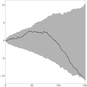
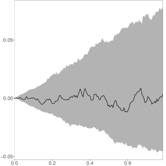
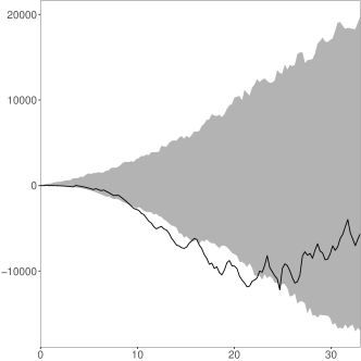
First, we considered the locations and orientations separately and used $\hat{K}_{1}$ and $\hat{K}_{2}$, respectively, as test functions for the global rank envelope procedure. Using 2499 simulations from a homogeneous Poisson process on $W$, we obtained a global rank envelope test with $p$-interval $(0.000,0.020)$. Thus, we reject that the locations follow a homogeneous Poisson model. The associated $95\%$ global rank envelopes in Figure 6 show that the rejection is due to the observed $\hat{K}_{1}(r)$ falling below the envelope for $r$-values between $10\text{\,}\mathrm{\SIUnitSymbolMicro m}25\text{\,}\mathrm{\SIUnitSymbolMicro m}$. This suggests that the observed locations exhibit some degree of regularity that needs to be modelled. For the orientations, a global rank envelope test based on 2499 simulations under an inhomogeneous Poisson model on $\mathbb{S}^{2}$ with intensity $\hat{\rho}_{2}(u)=n\hat{f}(u)$ gave a $p$-interval of $(0.475,0.481)$ and thus no evidence against the proposed model. Figure 6 shows the associated $95\%$ global rank envelope.

Figure 5: Plots of the observed neuron orientations (dots) and the fitted mixture density $\hat{f}$ (grey scale). Left: plot of orientations represented as cosine-colatitude and longitude along with their marginal histograms and marginal fitted densities (solid curves) found by numerically integrating $\hat{f}$. Right: stereographic projection of the northern (top) and southern (bottom) hemisphere.

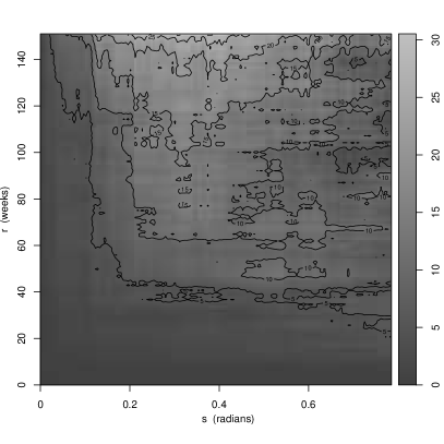
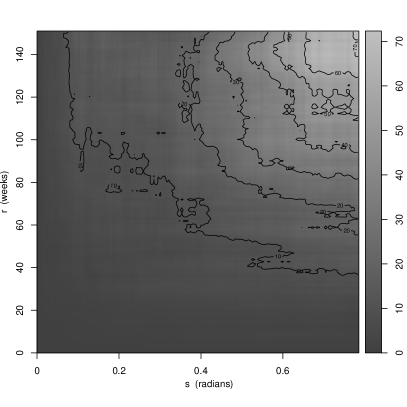
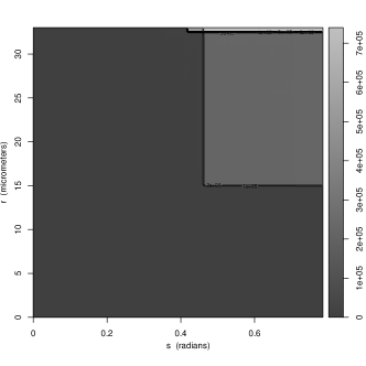
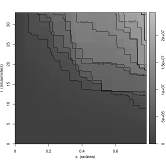
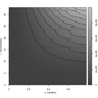
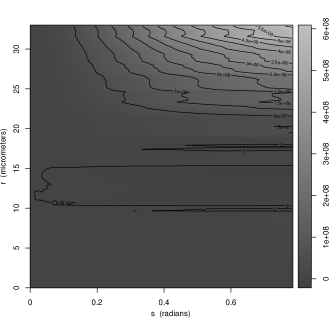
Second, we considered the data as a space-sphere point pattern and used $\hat{K}$ and $\hat{D}$ to test for a Poisson model with a separable intensity estimated by $\hat{\rho}(y,u)=\hat{\rho}_{1}\hat{\rho}_{2}(u)/n=n\hat{f}(u)/|W|$, cf. (4.1). As the test functions $\hat{K}(r,s)$ and $\hat{D}(r,s)$ depend on the two-dimensional argument $(r,s)$ and they are non-smooth with large jumps due to few orientations occurring in areas with low intensity, we increased the number of simulations to 49999 in order to improve the quality of the global rank envelope test (49999 is a much higher number than recommended in Myllymäki et al., 2017, for test functions depending on one argument only). This resulted in the $p$-intervals $(0.547,0.549)$ for $\hat{K}$ and $(0.000,0.003)$ for $\hat{D}$; plots of the difference between the associated envelopes and the observed test function are shown in Figure 7. In conclusion, the test based on $\hat{K}$ reveals no evidence against the proposed space-sphere Poisson model even though the corresponding Poisson model for the locations was rejected by the test based on $\hat{K}_{1}$. However, the test based on $\hat{D}$ provides a great deal of evidence against the model. This conclusion is probably due to the fact that for this data set $\hat{K}_{1}(r)\hat{K}_{2}(s)\gg\hat{K}(r,s)$, meaning that the test based on $\hat{D}$ is highly controlled by the values of $\hat{K}_{1}$ and $\hat{K}_{2}$, which cf. Figure 7 results in a rejection for $r$-values from $10\text{\,}\mathrm{\SIUnitSymbolMicro m}20\text{\,}\mathrm{\SIUnitSymbolMicro m}$, in line with the test based on $\hat{K}_{1}$.

It is unsatisfactory that $\hat{K}$ does not detect any deviation from Poisson when $\hat{K}_{1}$ clearly does, but we expect that the large jumps in $\hat{K}(r,s)$, caused by $(r,s)$-close neighbours with low intensity, may explain why no evidence against the model is detected. The few orientations that were modelled using a Watson distribution mostly fall in places with very low intensity. Therefore, we independently thinned the space-sphere point pattern with retention probability $\hat{p}\hat{f}_{K}(u)/\hat{f}(u)$ for $u\in\mathbb{S}^{2}$. Thereby (with high probability) we removed neurons with orientations that were most likely generated by the Watson distribution. This lead to removal of 26 neurons. For the thinned data, the global rank envelope test based on $\hat{K}$ for testing the hypothesis of an inhomogeneous Poisson process with intensity proportional to a Kent density gave a $p$-interval of $(0.052,0.058)$. Still, the model was not rejected at a $5\%$ significance level, but we at least got closer to a rejection; and so we continued the analysis with the thinned data. The analysis here indicates that, at least in some cases, the power of the global rank envelope test based on $\hat{K}$ may be small. This is investigated further in Section 6.3.

Figure 6: Left: $\hat{K}_{1}(r)-4\pi r^{3}/3$ for the neuron locations (solid curve) along with a 95% global rank envelope (grey area) under a homogeneous Poisson model on $W\subseteq\mathbb{R}^{3}$. Right: $\hat{K}_{2}(s)-2\pi\{1-\cos(s)\}$ for the neuron orientations (solid curve) along with a 95% global rank envelope (grey area) under the fitted inhomogeneous Poisson model on $\mathbb{S}^{2}$.

As we have seen, a homogeneous Poisson model is not adequate for the locations, and thus a Poisson model with intensity $\hat{\rho}$ as described above is not suitable for describing the space-sphere point pattern. To investigate whether orientations and locations can be modelled separately, that is, whether the locations and orientations are independent, we kept the locations fixed, and independent of the locations we simulated IID orientations from the fitted Kent distribution. The resulting global rank envelope test based on $49999$ of such simulations gave a $p$-interval of $(0.9255,0.9258)$ for $\hat{K}$ and $(0.1265,0.1266)$ for $\hat{D}$, showing no evidence against the hypothesis of independence between locations and orientations. Alternatively, if one does not have a suitable model to simulate the spherical (or spatial) components from, the independence test may be performed by randomly permuting the components. Formally, this tests only the hypothesis of exchangeability; a property that is fulfilled under independence. Performing such a permutation test for our data where the locations were fixed and the orientations permuted $49999$ times resulted in a $p$-interval of $(0.5431,0.5445)$ using either $\hat{K}$ or $\hat{D}$ (as $\hat{K}$ and $\hat{D}$ only differ by a constant under permutation of the orientations and thus lead to equivalent tests).

Figure 7: For $\hat{T}=\hat{K}$ (first row) and $\hat{T}=\hat{D}$ (second row): difference between $\hat{T}(r,s)$ for the observed neuron locations and orientations and the lower ($\hat{T}_{\mathrm{low}}$) or upper ($\hat{T}_{\mathrm{upp}}$) 95% global rank envelope under the fitted inhomogeneous Poisson model on $W\times\mathbb{S}^{2}$. Left: $\hat{T}(r,s)-\hat{T}_{\mathrm{low}}(r,s)$. Right: $\hat{T}_{\mathrm{upp}}(r,s)-\hat{T}(r,s)$.

6.3 Simulation study

In the data analyses in Sections 6.1–6.2, the tests based on $\hat{K}$ failed to reject the proposed Poisson models in cases where the corresponding spatial model was rejected when using $\hat{K}_{1}$. To investigate whether the space-sphere $K$-function is a valuable addition to the existing functional summary statistics on the space and sphere, we performed a simulation study comparing the power of global rank envelope tests based on either $\hat{K}$, $\hat{D}$, or a combination of $\hat{K}_{1}$ and $\hat{K}_{2}$. (The combined test function is simply a concatenation of $\hat{K}_{1}$ and $\hat{K}_{2}$. Mrkvička et al. (2017) recommended using such a combination rather than $\hat{K}_{1}$ or $\hat{K}_{2}$ as a test function.)

Specifically, we consider a homogeneous LGCP $X$ driven by a random field $\Lambda(y,u)=\rho\exp\{Z(y,u)\}$, where $\rho>0$ and

$$Z(y,u)=\alpha+\sigma_{1}Z_{1}(y)+\sigma_{2}Z_{2}(u)+\delta Z_{3}(y,u),\qquad y\in\mathbb{R},\ u\in\mathbb{S}^{2},$$

for parameters $\sigma_{1},\sigma_{2}>0$, $\delta\geq 0$, and $\alpha=-(\sigma_{1}^{2}+\sigma_{2}^{2}+\delta^{2})/2$. Further, $Z_{1},Z_{2}$, and $Z_{3}$ are independent GRFs with mean $0$ and covariance functions $c_{1}(y_{1},y_{2})=\exp(-\|y_{1}-\nobreak y_{2}\|_{d}/\phi_{1})$, $c_{2}(u_{1},u_{2})=\exp(-d(u_{1},u_{2})/\phi_{2})$, and $c_{3}(y_{1},u_{1},y_{2},u_{2})=\linebreak c_{1}(y_{1},y_{2})c_{2}(u_{1},u_{2})$, respectively, with parameters $\phi_{1},\phi_{2}>0$. Note that the resulting LGCP is homogeneous (and thus first order separable) and SOIRS for any value of $\delta\geq 0$. In addition, by (2.12), the process is second order separable if and only if $\delta=0$, in which case $X$ has pair correlation function

$$g_{\theta}(y_{1},u_{1},y_{2},u_{2})$$ (6.1)

$$=\exp\{\sigma_{1}^{2}c_{1}(y_{1},y_{2})+\sigma_{2}^{2}c_{2}(u_{1},u_{2})\},\qquad y_{1},y_{2}\in\mathbb{R},\ u_{1},u_{2}\in\mathbb{S}^{2},$$

where $\theta=(\sigma_{1},\phi_{1},\sigma_{2},\phi_{2})$.

For each value of $\delta=0,0.5,1,1.5,2$, we simulated 100 realisations of a LGCP on $[0,1]\times\mathbb{S}^{2}$ with $\rho=1000$, $\sigma_{1}=\sigma_{2}=0.5$, $\phi_{1}=0.05$, and $\phi_{2}=0.132$. Then for each of these simulations, we fitted the LGCP model with $\delta=0$ using a second order composite likelihood approach proposed by Guan (2006) to estimate $\theta$. In the present time-sphere setting, for a finite point pattern $x\subset[0,1]\times\mathbb{S}^{2}$, the log second order composite likelihood is given by

$$\mathrm{CL}(\theta;x)={} \sum_{(y_{i},u_{i}),(y_{j},u_{j})\in x}^{\neq}w(y_{i},u_{i},y_{j},u_{j})\log\{\rho^{\smash{(}2\smash{)}}_{\theta}(y_{i},u_{i},y_{j},u_{j})\}$$ (6.2)

$$-n_{r,s}\begin{aligned} \log\biggl{\{}&\int_{[0,1]\times\mathbb{S}^{2}}\int_{[0,1]\times\mathbb{S}^{2}}w(y_{1},u_{1},y_{2},u_{2})\\ &\cdot\rho^{\smash{(}2\smash{)}}_{\theta}(y_{1},u_{1},y_{2},u_{2})\,\mathrm{d}\mu(y_{1},u_{1})\,\mathrm{d}\mu(y_{2},u_{2})\biggr{\}}.\end{aligned}$$

Here, for user specified distances $r$ and $s$, $w(y_{1},u_{1},y_{2},u_{2})=\mathbb{I}\{\|y_{1}-y_{2}\|_{d}<r$, $d(u_{1},u_{2})<s\}$, $n_{r,s}$ is the number of $(r,s)$-close neighbours, and $\rho_{\theta}^{\smash{(}2\smash{)}}$ is the second order joint intensity function, which for the homogeneous LGCP presented above is $\rho_{\theta}^{\smash{(}2\smash{)}}(y_{1},u_{1},y_{2},u_{2})=\rho^{2}g_{\theta}(y_{1},u_{1},y_{2},u_{2})$. Then (6.2) is easily seen not to depend on $\rho$, and by (6.1) the composite likelihood can be written as

$$\mathrm{CL}(\theta;x)=l_{1}(\sigma_{1},\phi_{1};x)+l_{2}(\sigma_{2},\phi_{2};x)$$ (6.3)

for functions $l_{1}$ and $l_{2}$. Thus, maximising the composite likelihood with respect to $\theta$ can be split into two maximisation problems; that is, maximising $l_{1}$ with respect to $(\sigma_{1},\phi_{1})$ and $l_{2}$ with respect to $(\sigma_{2},\phi_{2})$. Finally, we tested the null hypothesis $\delta=0$ using the global rank envelope test with 4999 simulations from the fitted model using either $\hat{K}$, $\hat{D}$, or a combination of $\hat{K}_{1}$ and $\hat{K}_{2}$ as test functions.

Table 1 gives an overview of the conclusions reached by these tests. Note that the power of the tests based on either of the three test functions in general increases with $\delta$, both for the liberal and conservative test (for details see Appendix A). Thus, with increasing degree of non-separability the tests more often detect deviation from the separable model. However, tests based on $\hat{K}$ and particularly $\hat{D}$ seem preferable in this setup as they have a higher power than tests based on $\hat{K}_{1}$ combined with $\hat{K}_{2}$.

Obviously, the conservative $p$-value always lead to fewer rejections than the liberal, giving a lower power. However, if the global rank envelope procedure is based on a higher number of simulations, then the conservative and liberal test will more often lead to the same conclusion.

Table 1: Power of tests for different values of $\delta$ when using the global rank envelope test with either $\hat{K}$, $\hat{D}$, or $\hat{K}_{1}$ combined with $\hat{K}_{2}$. The decision was made using a significance level of $5\%$ for both the liberal and conservative tests.

	Test function	$\delta=0$	$\delta=0.5$	$\delta=1$	$\delta=1.5$	$\delta=2$
Liberal	$\hat{K}$	$4$%	$7$%	$42$%	$75$%	$98$%
	$\hat{D}$	$2$%	$45$%	$92$%	$97$%	$100$%
	$\hat{K}_{1},\hat{K}_{2}$	$10$%	$11$%	$29$%	$28$%	$42$%
Conservative	$\hat{K}$	$2$%	$5$%	$32$%	$72$%	$90$%
	$\hat{D}$	$0$%	$26$%	$77$%	$82$%	$86$%
	$\hat{K}_{1},\hat{K}_{2}$	$10$%	$11$%	$29$%	$28$%	$40$%

7 Additional comments

Section 2.2 introduced examples of space-sphere point processes for which the second order separability property described in Section 4 seems natural. However, for other classes of point processes a different structure of the pair correlation function may be more interesting. For example, suppose $X$ is a Cox process driven by

$$\Lambda(y,u)=\sum_{(y^{\prime},u^{\prime},\gamma^{\prime})\in\Phi}\gamma^{\prime}k(y^{\prime},u^{\prime},y,u),\qquad y\in\mathbb{R}^{d},\,u\in\mathbb{S}^{k},$$ (7.1)

where $\Phi$ is a Poisson process on $S\times(0,\infty)$ with intensity function $\zeta$, and $k(y^{\prime},u^{\prime},\cdot,\cdot)$ is a density with respect to $\mu$. Then $X$ is called a shot noise Cox process (SNCP) with kernel $k$ (Møller, 2003). The process has intensity function

$$\rho(y,u)=\iint\gamma^{\prime}\zeta(y^{\prime},u^{\prime},\gamma^{\prime})k(y^{\prime},u^{\prime},y,u)\,\mathrm{d}\mu(y^{\prime},u^{\prime})\,\mathrm{d}\gamma^{\prime},\qquad y\in\mathbb{R}^{d},\,u\in\mathbb{S}^{k},$$

and pair correlation function

$$g(y_{1},u_{1},y_{2},u_{2})$$ (7.2)

$$=1+\frac{\displaystyle\iint\gamma^{\prime 2}\zeta(y^{\prime},u^{\prime},\gamma^{\prime})k(y^{\prime},u^{\prime},y_{1},u_{1})k(y^{\prime},u^{\prime},y_{2},u_{2})\,\mathrm{d}\mu(y^{\prime},u^{\prime})\,\mathrm{d}\gamma^{\prime}}{\rho(y_{1},u_{1})\rho(y_{2},u_{2})}$$

for any $y_{1},y_{2}\in\mathbb{R}^{d}$ and any $u_{1},u_{2}\in\mathbb{S}^{k}$ with $\rho(y_{1},u_{1})\rho(y_{2},u_{2})>0$. In the trivial case where the kernel $k(y^{\prime},u^{\prime},y,u)$ in (7.1) does not depend on $u$ (or $y$), the SNCP is both first and second order separable, with intensity and pair correlation functions that do not depend on the spherical (or spatial) components, and the process thus fulfils second order separability in the sense of (4.2). However, the specific structure of the pair correlation function for a SNCP in (7.2) makes it more natural to look for a product structure in $g-1$ rather than $g$. That is, we may say that $X$ is second order separable if there exist Borel functions $h_{1}$ and $h_{2}$ such that

$$g(y_{1},u_{1},y_{2},u_{2})-1=h_{1}(y_{1},y_{2})h_{2}(u_{1},u_{2}),\qquad y_{1},y_{2}\in\mathbb{R}^{d},\,u_{1},u_{2}\in\mathbb{S}^{k}.$$ (7.3)

This property is naturally fulfilled whenever we consider a Poisson process or any marked point process with marks that are IID and independent of the ground process as described in Example 3. Now, think of $\Phi$ in (7.1) as a marked point process with ground process $\{(y,u):(y,u,\gamma)\in\Phi\}$ and marks $\{\gamma:(y,u,\gamma)\in\Phi\}$, and assume that the ground process and the marks are independent processes, the ground process is a homogeneous Poisson process on $S$ with intensity $\alpha>0$, and the marks are IID with mean $m_{1}$ and second moment $m_{2}$. If in addition $k(y^{\prime},u^{\prime},y,u)=k_{0}\{y-y^{\prime},\allowbreak d(u,u^{\prime})\}$, then $\Lambda$ and thus $X$ is stationary in space and isotropic on the sphere. Further, $X$ is homogeneous with intensity $\rho=m_{1}\alpha$ and pair correlation function

$$g(y_{1},u_{1},y_{2},u_{2})=1+\frac{m_{2}}{\alpha m_{1}^{2}}\int k_{0}\{y_{1}-y^{\prime},d(u_{1},u^{\prime})\}k_{0}\{y_{2}-y^{\prime},d(u_{2},u^{\prime})\}\,\mathrm{d}\mu(y^{\prime},u^{\prime})$$ (7.4)

for $y_{1},y_{2}\in\mathbb{R}^{d}$ and $u_{1},u_{2}\in\mathbb{S}^{k}$. Clearly, (7.4) depends only on $(y_{1},y_{2})$ through $y_{1}-y_{2}$, and on $(u_{1},u_{2})$ through $d(u_{1},u_{2})$, although there is no simple expression for these dependencies in general. Furthermore, separability in the form of (7.3) is fulfilled if the kernel $k$ in (7.4) factorizes such that

$$k_{0}\{y-y^{\prime},d(u,u^{\prime})\}=k_{01}(y-y^{\prime})k_{02}\{d(u,u^{\prime})\},\qquad y,y^{\prime}\in\mathbb{R}^{d},\,u,u^{\prime}\in\mathbb{S}^{k},$$

for Borel functions $k_{01}$ and $k_{02}$. Then by (2.6)–(2.9), the pair correlations functions for $Y$ and $U_{W}$ are

$$g_{1}(y_{1},y_{2}) =1+c_{1}\frac{m_{2}}{\alpha m_{1}^{2}}\int k_{01}(y_{1}-y^{\prime})k_{01}(y_{2}-y^{\prime})\,\mathrm{d}y^{\prime},\qquad y_{1},y_{2}\in\mathbb{R}^{d},$$

and

$$g_{2}(u_{1},u_{2}) =1+c_{2}\frac{m_{2}}{\alpha m_{1}^{2}}\int k_{02}\{d(u_{1},u^{\prime})\}k_{02}\{d(u_{2},u^{\prime})\}\,\mathrm{d}\nu(u^{\prime}),\qquad u_{1},u_{2}\in\mathbb{S}^{k},$$

where

$$c_{1} =\frac{1}{\sigma_{k}^{2}}\iiint k_{02}\{d(u_{1},u^{\prime})\}k_{02}\{d(u_{1},u^{\prime})\}\,\mathrm{d}\nu(u_{1})\,\mathrm{d}\nu(u_{2})\,\mathrm{d}\nu(u^{\prime})$$

and

$$c_{2} =\frac{1}{|W|^{2}}\int\int_{W}\int_{W}k_{01}(y_{1}-y^{\prime})k_{01}(y_{1}-y^{\prime})\,\mathrm{d}y_{1}\,\mathrm{d}y_{2}\,\mathrm{d}y^{\prime}.$$

That is, $g_{1}$ depends only on the spherical components through the constant $c_{1}$, and similarly $g_{2}$ depends only on the spatial components through $c_{2}$. Prokešová and Dvořák (2014) discuss how an analogue property can be exploited to estimate the parameters of space-time SNCPs using minimum contrast estimation for the projected processes. A similar procedure will be applicable for space-sphere point processes, but we have not investigated this further.

Section 5 considered the situation where the spatial components of $X$ are observed on a subset of $\mathbb{R}^{d}$ and the spherical components are observable on the entire sphere. In more general applications, the spherical components may only be observable on a subset of $\mathbb{S}^{k}$ leading to edge effects on the sphere too. To account for this, edge correction methods for the sphere should be used when estimating $K_{2}$ (see Lawrence et al., 2016) and $K$. If $X$ is observable on a product space $W_{1}\times W_{2}$, where $W_{1}\subset\mathbb{R}^{d}$ and $W_{2}\subset\mathbb{S}^{k}$, then an edge corrected estimate for $K$ may be obtained by combining edge corrected estimates for $K_{1}$ and $K_{2}$ analogous to (5.3). Concerning the specific choice of edge correction method, Baddeley et al. (2015) mentioned for planar point processes that, “So long as some kind of edge correction is performed …, the particular choice of edge correction technique is usually not critical”. We expect that the situation is similar for our setting.

For one-dimensional test functions, Myllymäki et al. (2017) recommend using 2499 simulations to perform a global rank envelope test, and Mrkvička et al. (2017) discuss the appropriate number of simulations when using a multivariate test function (as the empirical space-sphere $K$-function). In Section 6.2, we used 49999 simulations for the global rank envelope test based on $\hat{K}$, since $\hat{K}$ had steep jumps. To avoid this large number of simulations, a refinement of the global rank envelope test discussed in Mrkvička et al. (2018) can be applied.

In Example 1 we noticed that if a space-sphere point process is a Poisson process, then the spatial and spherical components are Poisson processes as well. Nevertheless, using $\hat{K}$ for testing a space-sphere Poisson model may lead to a different conclusion than using $\hat{K}_{1}$ and $\hat{K}_{2}$ for testing whether the corresponding Poisson models for the spatial and spherical components, respectively, are appropriate. Indeed, in the case of Figures 3–4, the test based on $\hat{K}_{1}$ showed some evidence against a homogeneous Poisson model for the fireball event times, while no evidence against a homogeneous Poisson model for the locations over time was seen with the test based on $\hat{K}$. This observation together with the results in Section 6.2 was our motivation for making the simulation study in Section 6.3, where we investigated the power of global rank envelope tests based on either $\hat{K}$, $\hat{D}$, or a combination of $\hat{K}_{1}$ and $\hat{K}_{2}$, and we concluded that tests based on $\hat{K}$ and in particular $\hat{D}$ seem preferable.

In Section 6.3, we utilised homogeneity and second order separability to speed up optimisation of the second order composite likelihood proposed in Guan (2006). If the process is inhomogeneous but first (and second) order separable, we still get a separation of the composite likelihood similar to $\eqref{eq:CL_sep}$, where $l_{1}$ and $l_{2}$ now may depend also on intensity parameters. As an alternative, the second order composite likelihood discussed in Waagepetersen (2007) can be used. However, in that case, first and second order separability do not yield a separable likelihood as in (6.3), and for our simulation study it resulted in unstable estimates (and thus it was discarded in favour of the one proposed by Guan, 2006). Furthermore, one may investigate whether the adaptive procedure discussed in Lavancier et al. (2018) will provide stable estimates in the space-sphere setting. In short, Lavancier et al. (2018) consider the score function related to (6.2) and introduce a modified weight function $w$ depending on $g$.

In this paper, we considered point processes living on $\mathbb{R}^{d}\times\mathbb{S}^{k}$. Naturally, we may extend the results/methods to more general metric spaces $\mathbb{R}^{d}\times\mathbb{M}$, where $\mathbb{M}$ is a compact set (e.g. a torus). However, we need to require some invariance property for the metric space $\mathbb{M}$ and its metric under a group action, such that we can define an equivalence of the SOIRS property needed to define $K$.

Acknowledgements.

The authors are grateful to Jiří Dvořák for helpful comments and to Ali H. Rafati for collecting the pyramidal cell data. This work was supported by The Danish Council for Independent Research | Natural Sciences, grant DFF – 7014-00074 “Statistics for point processes in space and beyond”, and by the “Centre for Stochastic Geometry and Advanced Bioimaging”, funded by grant 8721 from the Villum Foundation.

Appendix A

In Sections 6.1–6.3, we used the global rank envelope test presented in Myllymäki et al. (2017) to test for various point process models. In this appendix, we briefly explain the idea and use of such a test. A global rank envelope test compares a chosen test function for the observed data with the distribution of the test function under the null model; as this distribution is typically unknown it is approximated using a Monte Carlo approach. The comparison is based on a rank that only gives a weak ordering of the test functions. Thus, instead of a single $p$-value, the global rank envelope test provides an interval of $p$-values, where the end points specify the most liberal and conservative $p$-values of the test. A narrow $p$-interval is desirable as the test is inconclusive if the $p$-interval contains the chosen significance level. The width of the $p$-interval depends on the number of simulations, smoothness of the test functions and dimensionality. Myllymäki et al. (2017) recommended to use 2499 simulations for one-dimensional test functions and a significance level of $5\%$.

An advantage of the global rank envelope procedure is that it provides a graphical interpretation of the test in form of critical bounds (called a global rank envelope) for the test function. For example, if the observed test function is not completely inside the $95\%$ global rank envelope, this corresponds to a rejection of the null hypothesis at a significance level of $5\%$. Furthermore, locations where the observed test function falls outside the global rank envelope reveal possible reasons for rejecting the null model.

In their supplementary material, Myllymäki et al. (2017) discussed two approaches for calculating test functions that rely on an estimate of the intensity. One approach is to reuse the intensity estimate for the observed point pattern in calculation of all the test functions, another is to reestimate the intensity for each simulation and then use this estimate when calculating the associated test function. For the $L$-function, which is a transformation of $K_{1}$, Myllymäki et al. (2017) concluded that the reestimation approach give the more powerful test. In this paper, we have therefore based all our global rank envelope tests on that approach.

References

- Baddeley et al. (2000) Baddeley A, Møller J, Waagepetersen R (2000) Non- and semi-parametric estimation of interaction in inhomogeneous point patterns. Stat Neerl 54:329–350
- Baddeley et al. (2015) Baddeley A, Rubak E, Turner R (2015) Spatial Point Patterns: Methodology and Applications with R. Chapman & Hall/CRC Press, Boca Raton
- Baddeley et al. (2017) Baddeley A, Nair G, Rakshit S, McSwiggan G (2017) “Stationary” point processes are uncommon on linear networks. Stat 6:68–78
- Buxhoeveden and Casanova (2002) Buxhoeveden DP, Casanova MF (2002) The minicolumn hypothesis in neuroscience. Brain 125:935–951
- Cox (1955) Cox DR (1955) Some statistical models related with series of events. J R Stat Soc Ser B 17:129–164
- Daley and Vere-Jones (2003) Daley DJ, Vere-Jones D (2003) An Introduction to the Theory of Point Processes. Volume I: Elementary Theory and Methods, 2nd edn. Springer-Verlag, New York
- Diggle (2014) Diggle P (2014) Statistical Analysis of Spatial and Spatio-temporal Point Patterns. Chapman & Hall/CRC Press, Boca Raton
- Diggle et al. (1995) Diggle P, Chetwynd A, Häggkvist R (1995) Second-order analysis of space-time clustering. Stat Methods Med Res 4:124–136
- Dvořák and Prokešová (2016) Dvořák J, Prokešová M (2016) Parameter estimation for inhomogeneous space-time shot-noise Cox point processes. Scand J Stat 43:939–961
- Fisher et al. (1987) Fisher NI, Lewis T, Embleton BJJ (1987) Statistical Analysis of Spherical Data. Cambridge University Press, New York
- Gabriel and Diggle (2009) Gabriel E, Diggle P (2009) Second-order analysis of inhomogeneous spatio-temporal point process data. Stat Neerl 63:43–51
- Guan (2006) Guan Y (2006) A composite likelihood approach in fitting spatial point process models. J Amer Stat Assoc 101:1502–1512
- Illian et al. (2008) Illian J, Penttinen A, Stoyan H, Stoyan D (2008) Statistical Analysis and Modelling of Spatial Point Patterns. Statistics in Practice, Wiley, Chichester
- Koubek et al. (2016) Koubek A, Pawlas Z, Brereton T, Kriesche B, Schmidt V (2016) Testing the random field model hypothesis for random marked closed sets. Spat Stat 16:118–136
- Lavancier et al. (2015) Lavancier F, Møller J, Rubak E (2015) Determinantal point process models and statistical inference. J R Stat Soc Ser B 77:853–877
- Lavancier et al. (2018) Lavancier F, Poinas A, Waagepetersen R (2018) Adaptive estimating function inference for non-stationary determinantal point processes, available on arXiv:1806.06231
- Lawrence et al. (2016) Lawrence T, Baddeley A, Milne R, Nair G (2016) Point pattern analysis on a region of a sphere. Stat 5:144–157
- Li (2011) Li S (2011) Concise formulas for the area and volume of a hyperspherical cap. Asian J Math Stat 4:66–70
- Lorente de Nó (1938) Lorente de Nó R (1938) The cerebral cortex: Architecture, intracortical connections, motor projections. In: Fulton JF (ed) Physiology of the Nervous System, Oxford University Press, Oxford, pp 274–301
- Møller (2003) Møller J (2003) Shot noise Cox processes. Adv Appl Probab 35:614–640
- Møller and Ghorbani (2012) Møller J, Ghorbani M (2012) Aspects of second-order analysis of structured inhomogeneous spatio-temporal point processes. Stat Neerl 66:472–491
- Møller and Rubak (2016) Møller J, Rubak E (2016) Functional summary statistics for point processes on the sphere with an application to determinantal point processes. Spat Stat 18:4–23
- Møller and Waagepetersen (2004) Møller J, Waagepetersen R (2004) Statistical Inference and Simulation for Spatial Point Processes. Chapman & Hall/CRC Press, Boca Raton
- Møller and Waagepetersen (2007) Møller J, Waagepetersen R (2007) Modern statistics for spatial point processes. Scand J Stat 34:643–684
- Møller et al. (1998) Møller J, Syversveen AR, Waagepetersen RP (1998) Log Gaussian Cox processes. Scand J Stat 25:451–482
- Møller et al. (2018) Møller J, Nielsen M, Porcu E, Rubak E (2018) Determinantal point process models on the sphere. Bernoulli 24:1171–1201
- Mountcastle (1978) Mountcastle VB (1978) The Mindful Brain: Cortical Organization and the Group-selective Theory of Higher Brain Function. MIT Press, Cambridge
- Mrkvička et al. (2017) Mrkvička T, Myllymäki M, Hahn U (2017) Multiple Monte Carlo testing, with applications in spatial point processes. Stat Comput 27:1239–1255
- Mrkvička et al. (2018) Mrkvička T, Hahn U, Myllymäki M (2018) A one-way anova test for functional data with graphical interpretation, available on arXiv:1612.03608
- Myllymäki et al. (2017) Myllymäki M, Mrkvička T, Grabarnik P, Seijo H, Hahn U (2017) Global envelope tests for spatial processes. J R Stat Soc Ser B 79:381–404
- Ohser (1983) Ohser J (1983) On estimators for the reduced second moment measure of point processes. Mathematische Operationsforschung und Statistik, Series Statistics 14:63–71
- Prokešová and Dvořák (2014) Prokešová M, Dvořák J (2014) Statistics for inhomogeneous space-time shot-noise Cox processes. Spat Stat 10:76–86
- Waagepetersen (2007) Waagepetersen R (2007) An estimating function approach to inference for inhomogeneous Neyman-Scott processes. Biometrics 63:252–258