Primordial Non-Gaussianity

Abstract

Here we review the present status of modelling of and searching for primordial non-Gaussianity of cosmological perturbations. After introducing the models for non-Gaussianity generation during inflation, we discuss the search for non-Gaussian signatures in the Cosmic Microwave Background and in the Large-Scale Structure of the Universe.

1 Introduction

According to Planck 2018, “the 6-parameter $\Lambda$CDM model provides an astonishingly accurate description of the Universe form times prior to  380,000 years after the Big Bang, defining the last-scattering surface observed via the Cosmic Microwave Background (CMB) radiation, to the present day at an age of 13.8 billion years” [1].
Actually, the concordance model describes the evolution of tiny fluctuations on top of a homogeneous and isotropic background from the early Universe to the time of observation. Specifically, we can study how these modes looked like at the last-scattering surface, by analyzing the inhomogeneities in the CMB, and, in recent times, by observing the Large-Scale Structure (LSS) of the Universe.

In the standard model of cosmology, the primordial perturbations, corresponding to the seeds for the LSS, are chosen from a Gaussian distribution with random phases. This assumption is justified from experimental evidences as deviations from this Gaussian hypothesis, i.e. Primordial Non-Gaussianity (PNG), have not been observed yet.
Note that from the theoretical point of view, it is not surprising that “a Gaussian random field may provide a good description of the properties of density fluctuations” [2]. Actually, “the central limit theorem implies that a Gaussian distribution arises whenever one has a variable […] which is a linear superposition of a large number of independent random variables […] which are all drawn from the same distribution” [2].
For this reason, deviations from perfect Gaussianity can provide relevant information on the early Universe and research on PNG is particularly important, especially if these initial conditions were generated by some dynamical process, such as, for example, inflation in the Early Universe.
Actually, while “small-amplitude curvature perturbations generated by quantum fluctuations in an inflationary phase […] would yield a nearly Gaussian random density field” [2], direct measurements of non-Gaussianity would allow us to go beyond the free-field limit, providing information concerning the degrees of freedom, the possible symmetries and the interactions characterizing the inflationary action.

1.1 Historical outline

To be, or not to be Gaussian? The quest for Non-Gaussianity (NG) has a long story, already during the late seventies observations indicated that the patterns in the LSS could not be related to a Gaussian distribution. More precisely, NG in the LSS was measured in 1977 by Groth and Peebles [3] who computed the 3-point function of galaxies, raising the question whether this feature was only associated to non-linear gravitational clustering or it also included some signature of primordial NG.

In the subsequent years, and especially during the late eighties, the consequences of strongly non-Gaussian initial conditions were investigated in order to explore alternative structure formation models. However, these extreme possibilities were later excluded by CMB and LSS observations with increased accuracy.

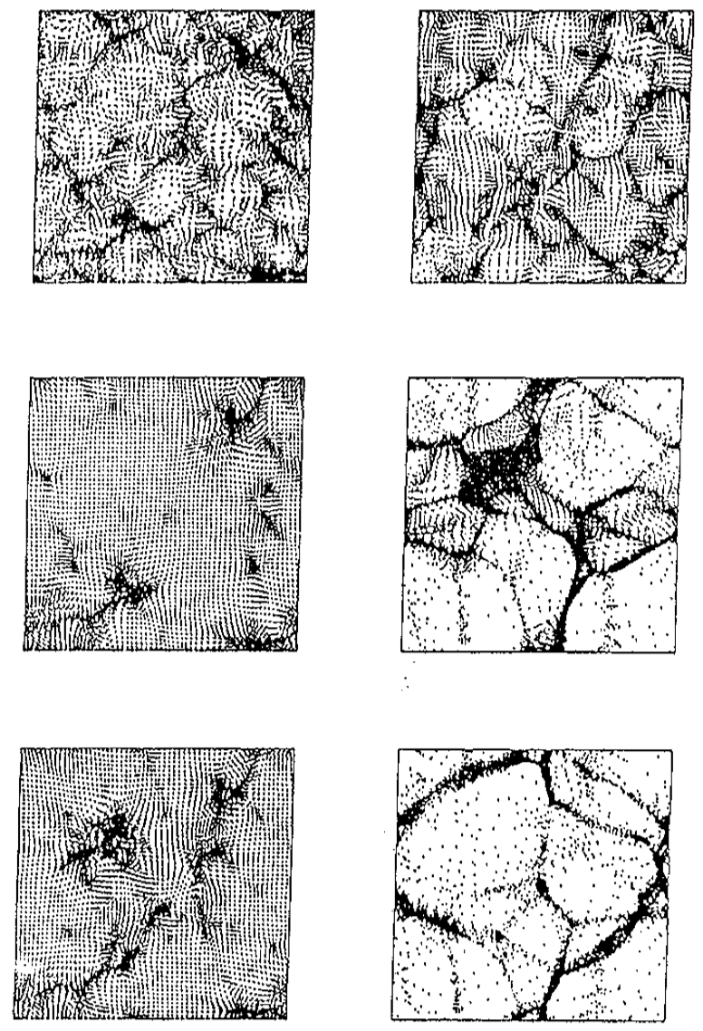
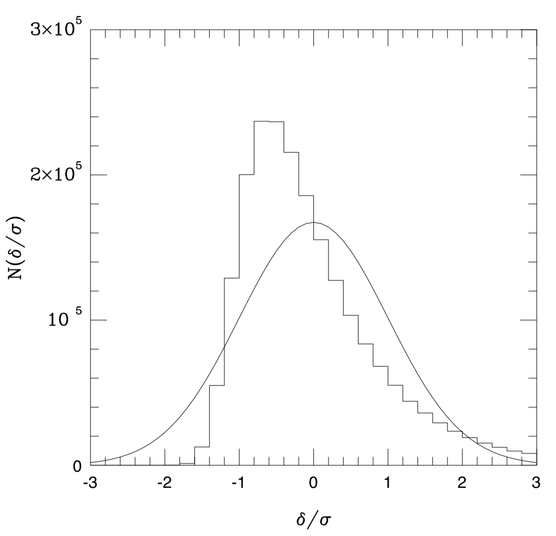
Remarkably, the early nineties featured the beginning of a new era of non-Gaussian models from inflation, characterized by a small $f_{\rm NL}$, compatible with observations [4, 5, 6, 7, 8]. At the same time, N-body simulations started to play a crucial role determining the LSS of the Universe arising from the non-linear gravitational clustering of non-Gaussian Cold Dark Matter perturbations. The view on NG using N-body simulations around 1990 can be depicted in Figure 1.

Figure 1: Projected particle positions in slices of depth one sixteenth of the computational box-size at the present time $t_{0}$. The slices refer to different models. From [9].

From the theoretical point of view, this line of research continued until the new millennium, when PNG finally emerged as a new “smoking gun” of (non-standard) inflation models [10, 11], probing interactions among fields at the highest energy scales, which complements the search for primordial gravitational-waves (PGW).

As for the experimental and observational side, the bispectra for PSCz[12] and the IRAS [13] redshift catalogues were determined in 2001, and for 2dF galaxies in 2002 [14]. More recently, the three-point correlation functions for the WiggleZ spectroscopic galaxy survey and the Baryon Oscillation Spectroscopic Survey were determined in [15] and [16, 17], respectively.

Finally, the very stringent Planck constraints on PNG [26, 27] rose the question whether this route is still viable or not, and the present-day challenge is to detect (or constrain) mild or weak deviations from primordial Gaussian initial conditions.

2 Non-Gaussianity in the Initial Conditions

The inflationary paradigm, a phase of accelerated expansion in the early Universe, was originally proposed at the end of the seventies in order to overcome some inconsistencies of the hot Big Bang model, which was plagued by the so-called flatness and horizon problems. At the same time, inflation suggested a quantum origin for the density fluctuations in the Universe, thereby providing a convincing dynamical mechanism for structure formation. Generally, the testable predictions of inflationary models are

• a critical value for the total energy density;

• almost, but not exact, scale-invariant and nearly Gaussian adiabatic density fluctuations;

• almost, but not exact, scale-invariant stochastic background of relic gravitational waves.

Note that Planck data have confirmed these predictions, for example the measured spectral index of the scalar power spectrum is $n_{s}=0.9649\pm 0.0042$ at 68% CL and no evidence for a scale dependence of $n_{s}$ has been found [28].
Also spatial flatness is confirmed at a precision of 0.4% at 95% CL with the combination of BAO data [28]. Prospects for further improving measurements of spatial curvature are discussed in [29].
While primordial gravitational waves have not been yet detected, the upper limit on the tensor-to-scalar ratio from the BICEP2/Keck CMB polarization experiments is $r_{0.05}<0.07$ at 95% confidence, which tightens to $r_{0.05}<0.06$ in conjunction with Planck temperature measurements and other data [28, 30].

In order to reconstruct the inflationary action, we need two ingredients:

• the stochastic GW background, providing information on the inflationary energy scales;

• deviations from Gaussian initial conditions, providing information on the possible interactions. Moreover, PNG features can help us to distinguish inflation models which would yield the same predictions for $n_{s}$ and $r$.

Many primordial (inflationary) models of non-Gaussianity can be represented in configuration space by the simple formula [4, 5, 6, 7, 8]

$$\Phi=\varphi_{L}+f_{\rm NL}\left(\varphi_{L}^{2}-\left<\varphi_{L}^{2}\right>\right)+g_{\rm NL}\left(\varphi_{L}^{3}-\left<\varphi_{L}^{2}\right>\varphi_{L}\right)+\dots$$ (1)

where $\Phi$ is the large-scale gravitational potential (or equivalently in terms of the gauge-invariant comoving curvature perturbation $\zeta$ which on super-horizon scales satisfies the relation $\Phi=3\,\zeta/5$), $\varphi_{L}$ its linear Gaussian contribution and $f_{\rm NL}$ the dimensionless non-linearity parameter (or more generally non-linearity function).

2.1 Non-Gaussianity and higher-order statistics

The simplest statistics measuring NG is the 3-point function or its Fourier transform, the “bispectrum”:

$$\left<\Phi(\mathbf{k}_{1})\Phi(\mathbf{k}_{2})\Phi(\mathbf{k}_{3})\right>=(2\pi)^{3}\delta^{(3)}(\mathbf{k}_{1}+\mathbf{k}_{2}+\mathbf{k}_{3})B_{\Phi}(k_{1},k_{2},k_{3})$$ (2)

which carries shape information. In the simple linear and quadratic model, parametrized by $\varphi_{L}$ and $f_{\rm NL}$, the bispectrum of the gravitational potential reads

$$B_{\Phi}(k_{1},k_{2},k_{3})=2f_{\rm NL}[P_{\Phi}(k_{1})P_{\Phi}(k_{1})+\text{cyclic terms}]$$ (3)

where we applied the Wick’s theorem and

$$\left<\Phi(\mathbf{k}_{1})\Phi(\mathbf{k}_{2})\right>=(2\pi)^{3}\delta^{(3)}(\mathbf{k}_{1}+\mathbf{k}_{2})P_{\Phi}(k_{1})\,.$$ (4)

In order to evaluate NG from the early Universe to the present time, we need, first of all, to calculate non-Gaussianity during inflation using a self-consistent method.
Then, we need to evolve scalar (vector) and tensor perturbations to second order outside the horizon, matching conserved second-order gauge-invariant variables, such as the comoving curvature perturbation $\zeta^{(2)}$ (or non-linear generalizations of it), to its value at the end of inflation (accurately accounting for reheating).
Finally, we consistently study the evolution of the perturbations after they re-entered the Hubble radius, by computing the second-order radiation transfer function for the CMB and the second-order matter transfer function for the LSS.

Although this procedure is involved, PNG represents a fundamental tool to probe fundamental physics (e.g. UV completion of the standard model of particle physics or general relativity such as string theory) during inflation at energies from the Grand Unified Theories (GUT) scale $\sim 10^{15}$ GeV to the Planck scale $\sim 10^{19}$ GeV, as different inflationary models predict different amplitudes and shapes of the bispectrum. For example, even tough standard models of slow-roll inflation predict tiny deviations from Gaussianity [4, 5, 6, 7, 8, 10, 11], consistent with the 2013 and 2015 Planck results, specific oscillatory PNG features can point to particular string-theory models as shown in [31, 32].

In conclusion, searching for PNG is interesting per-se for theoretically well-motivated models of inflation and, as shown in Planck 2015 results [27] (see also [28]), can severely limit various classes of inflationary models beyond the simplest paradigm.

2.2 Bispectrum of a self-interacting scalar field in de Sitter space

Consider a scalar field $\chi$ with cubic self-interactions, i.e. with an interaction term of the form $\lambda\,\chi^{3}/6$ in the Lagrangian.
Writing the field as $\chi=\chi_{0}+\delta\chi$, where $\delta\chi$ represent the fluctuations around its vacuum expectation value $\chi_{0}=\left<0|\chi|0\right>$, the two and three-point functions in Fourier space [33, 6, 34], after the rescaling $\delta\chi=\delta\hat{\chi}/a$ are given by

$$\left<0|\delta\hat{\chi}(\tau,\mathbf{k})\delta\hat{\chi}(\tau^{\prime},\mathbf{k}^{\prime})|0\right> =\delta^{(3)}(\mathbf{k}+\mathbf{k}^{\prime})G(k,\tau,\tau^{\prime})$$ (5)

$$\left<\delta\hat{\chi}_{\mathbf{k}_{1}}\delta\hat{\chi}_{\mathbf{k}_{2}}\delta\hat{\chi}_{\mathbf{k}_{3}}\right> =i\,\lambda\,\delta^{(3)}(\mathbf{k}_{1}+\mathbf{k}_{2}+\mathbf{k}_{3})\times$$

$$\times\int_{-\infty}^{\tau}\frac{d\tau^{\prime}}{H\tau^{\prime}}\left[\prod_{i=1}^{3}G(k_{i},\tau,\tau^{\prime})-\prod_{i=1}^{3}G^{\ast}(k_{i},\tau,\tau^{\prime})\right]$$

where the Green’s function reads

$$G(k_{i},\tau,\tau^{\prime})=\frac{1}{2k_{i}}\left(1-\frac{i}{k_{i}\tau}\right)\left(1+\frac{i}{k_{i}\tau^{\prime}}\right)e^{ik_{i}(\tau^{\prime}-\tau)}\,.$$ (6)

The bispectrum is ($\zeta$ being a function of order $1$)

$$\left<\delta\chi_{\mathbf{k}_{1}}\delta\chi_{\mathbf{k}_{2}}\delta\chi_{\mathbf{k}_{3}}\right>=\sum_{i}\nu_{3}(k_{i})\prod_{j\neq i}\frac{H^{2}}{2k_{j}^{3}}$$ (7)

where

$$\nu_{3}(k_{i})=\frac{\lambda}{3H^{2}}\left[\gamma+\zeta(k_{i})+\log(-k_{T}\tau)\right]\,.$$ (8)

Historically, in [33] it was found $f_{\rm NL}\sim\epsilon^{2}$ for the standard single-field slow-roll scenario (from non-linearity in the inflaton potential in a fixed de Sitter space-time).
Later, calculations from second-order gravitational corrections during stochastic inflation indicated $f_{\rm NL}\sim\epsilon,\eta$ [6]. This result has been confirmed in [10, 11], up to numerical factors and momentum-dependent terms, with a full second-order approach.
Finally, Weinberg extended the calculation of the bispectrum to 1-loop [35]. Remarkably, one of the terms gives rise to the so-called “consistency relation”, according to which $f_{\rm NL}=-5\,(n_{s}-1)/12$.
However, it has been shown that the “consistency relation” term can be gauged away by a non-linear rescaling of coordinates, up to sub-leading terms. Hence the only residual term is proportional to $\epsilon$ i.e. to the amplitude of tensor modes; see comments on this point, later on.

2.3 Shapes of non-Gaussianity from inflation

In order to extract the relevant information regarding the amplitude and shape of PNG, it is convenient to write the bispectrum of primordial curvature perturbations as

$$\left<\zeta(\mathbf{k}_{1})\zeta(\mathbf{k}_{2})\zeta(\mathbf{k}_{3})\right>=(2\pi)^{3}\delta^{(3)}(\mathbf{k}_{1}+\mathbf{k}_{2}+\mathbf{k}_{3})f_{\rm NL}F(k_{1},k_{2},k_{3})$$ (9)

where $f_{\rm NL}$ represents the amplitude, while $F(k_{1},k_{2},k_{3})$ encodes the shape of PNG. Note that, usually, we study the function $F(1,x_{2},x_{3})x_{2}^{2}x^{2}_{3}$ in terms of the rescaled coordinates $x_{2}=k_{2}/k_{1}$ and $x_{3}=k_{3}/k_{1}$, where momenta satisfy the triangle inequality $x_{2}+x_{3}>1$.

Remarkably, there are several possible shapes of non-Gaussianity from inflation, say more than … stars in the sky. The most famous are:

• local NG, characteristic for multi-field, curvaton, ekpyrotic and cyclic models;

• equilateral NG, associated to non-canonical kinetic and higher-derivative terms, DBI and K-inflation, ghost inflation and EFT approaches;

• orthogonal NG, which distinguishes between variants of non-canonical kinetic term and higher-derivative interactions;

• flattened or folded NG.

Figure 2: Plot of the function $F(1,x_{2},x_{3})x_{2}^{2}x^{2}_{3}$ for the local distribution. The figure is normalized to have value $1$ for equilateral configurations $x_{2}=x_{3}=1$ and set to zero outside the region $1-x_{2}\leq x_{3}\leq x_{2}$. From [36].

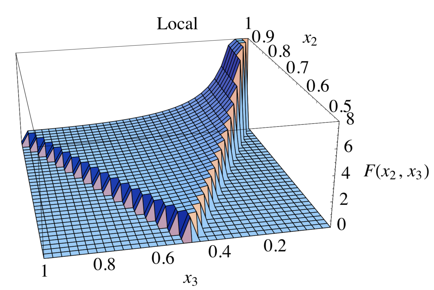
More specifically, the bispectrum for the local shape [4, 6, 7, 8] peaks for squeezed triangles $k_{3}\ll k_{1}\sim k_{2}$, see Figure 2. In this case, non-linearities develop outside the horizon during or immediately after inflation (e.g. multifield models of inflation).

Figure 3: Plot of the function $F(1,x_{2},x_{3})x_{2}^{2}x^{2}_{3}$ for non-Gaussianities generated by higher derivative interactions. From [37].

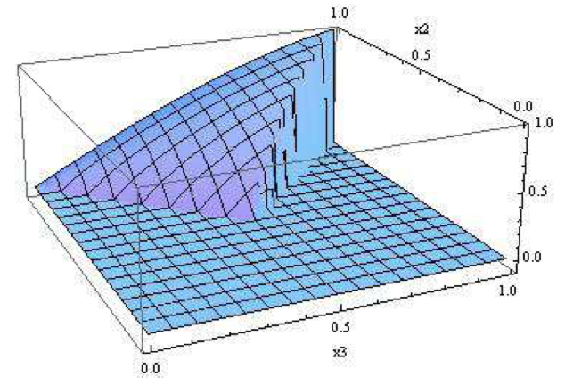
On the other hand, the bispectrum for the equilateral shape [38], see Figure 3, peaks for equilateral triangles $k_{1}=k_{2}=k_{3}$. Generally, in the equilateral family we can find single field models of inflation with non-canonical kinetic term $\mathcal{L}=P(\phi,X)$ with $X=-\frac{1}{2}\partial_{\mu}\phi\,\partial^{\mu}\phi$ (e.g. DBI or K-inflation) where NG comes from higher derivative interactions of the inflaton field, such as

$$\mathcal{L}\supset\delta\dot{\phi}(\nabla\delta\phi)^{2}\,.$$ (10)

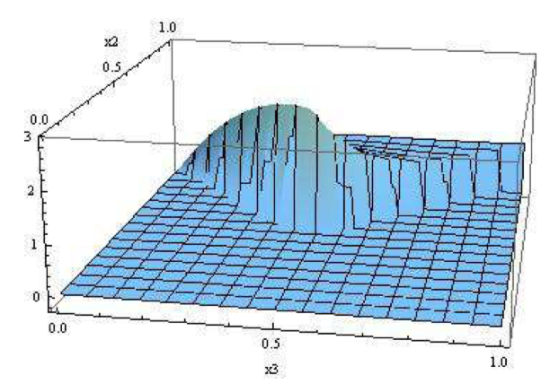
Finally, the bispectrum for the flattened shape peaks for flattened (or folded) triangles $k_{1}=k_{2}+k_{3}$, see Figure 4, and can be written in terms of the equilateral and orthogonal shapes [39]. It is characteristic for excited initial states (see [40, 41, 42]), higher derivative interactions [37] or models where a Galilean symmetry is imposed [43].

Figure 4: The folded template shape $F(x_{2},x_{3})x_{2}^{2}x^{2}_{3}$, the maximum is in the flat configuration ($k_{1}=1$, $k_{2}=k_{3}=\frac{1}{2}$). From [37].

However, there are many other shapes: e.g. directionally dependent bispectra, tensor bispectra, etc.

2.4 The role of $f_{\rm NL}$ and the detection of primordial non-Gaussianity

Clearly, detecting a non-zero primordial bispectrum (e.g. $f_{\rm NL}\neq 0$) proves that the initial seeds were non-Gaussian. Similarly, for the trispectrum and $n$-point correlation functions.
However, the opposite is not true, namely detecting $f_{\rm NL}\approx 0$ doesn’t prove Gaussianity. Actually, there are infinitely many ways PNG can evade observational bounds optimized to search for $f_{\rm NL}$ and similar higher-order parameters.
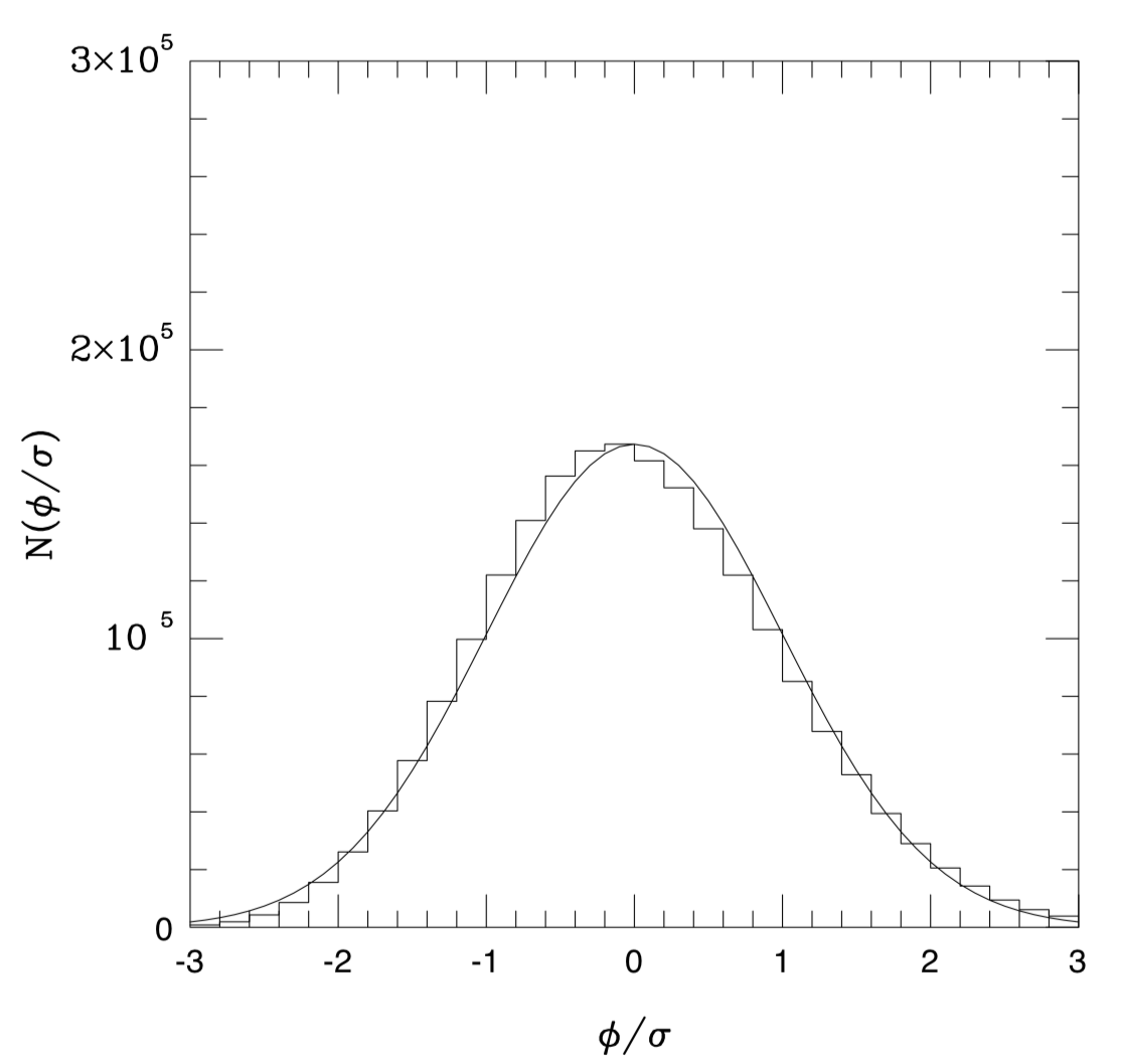
As an example, consider the situation where the linear density contrast $\delta$ is non-Gaussian [44]. In this case, by the central limit theorem, the gravitational potential $\Phi$ (which yields large-scale CMB anisotropies) tends to be much more Gaussian. Indeed, consider the non-Gaussian distribution of densities [44]

$$\delta(\mathbf{r})=\int f(|\mathbf{r}-\mathbf{r}^{\prime}|)\Delta(\mathbf{r}^{\prime})d^{3}\mathbf{r}^{\prime}$$ (11)

where $\Delta(\mathbf{r})$ is an uncorrelated field with a gamma distribution, and $f$ is chosen to give a Zel’dovich power spectrum ($P(k)\propto k$) for the density field. By solving Poisson’s equation, we get for the gravitational potential

$$\Phi(\mathbf{r})=-Ga^{2}\bar{\rho}\int\frac{\delta(\mathbf{r}^{\prime})d^{3}\mathbf{r}^{\prime}}{|\mathbf{r}-\mathbf{r}^{\prime}|}$$ (12)

with the resulting distribution very close to be Gaussian, see Figure 5.

Figure 5: On the left, the distribution of densities. Solid curve is a Gaussian distribution with the same mean and variance. On the right, the distribution of potentials for the same model. Solid curve is a Gaussian distribution with the same mean and variance. From [44].

3 Non-Gaussianity and Cosmic Microwave Background

As mentioned before, the Planck satellite has provided accurate measurements of higher-order CMB correlations, resulting in very stringent constraints on PNG.
Planck is a project of the European Space Agency, with instruments provided by two scientific Consortia funded by ESA member states (in particular the lead countries: France and Italy) with contributions from NASA (USA), and telescope reflectors provided in a collaboration between ESA and a scientific Consortium led and funded by Denmark.

Figure 6: Left column: temperature and polarization intensity Gaussian CMB simulations. Right column: temperature and polarization non-Gaussian maps with the same Gaussian seed as in the left column and $f_{\rm NL}=3000$. Temperatures are in mK. From [45].

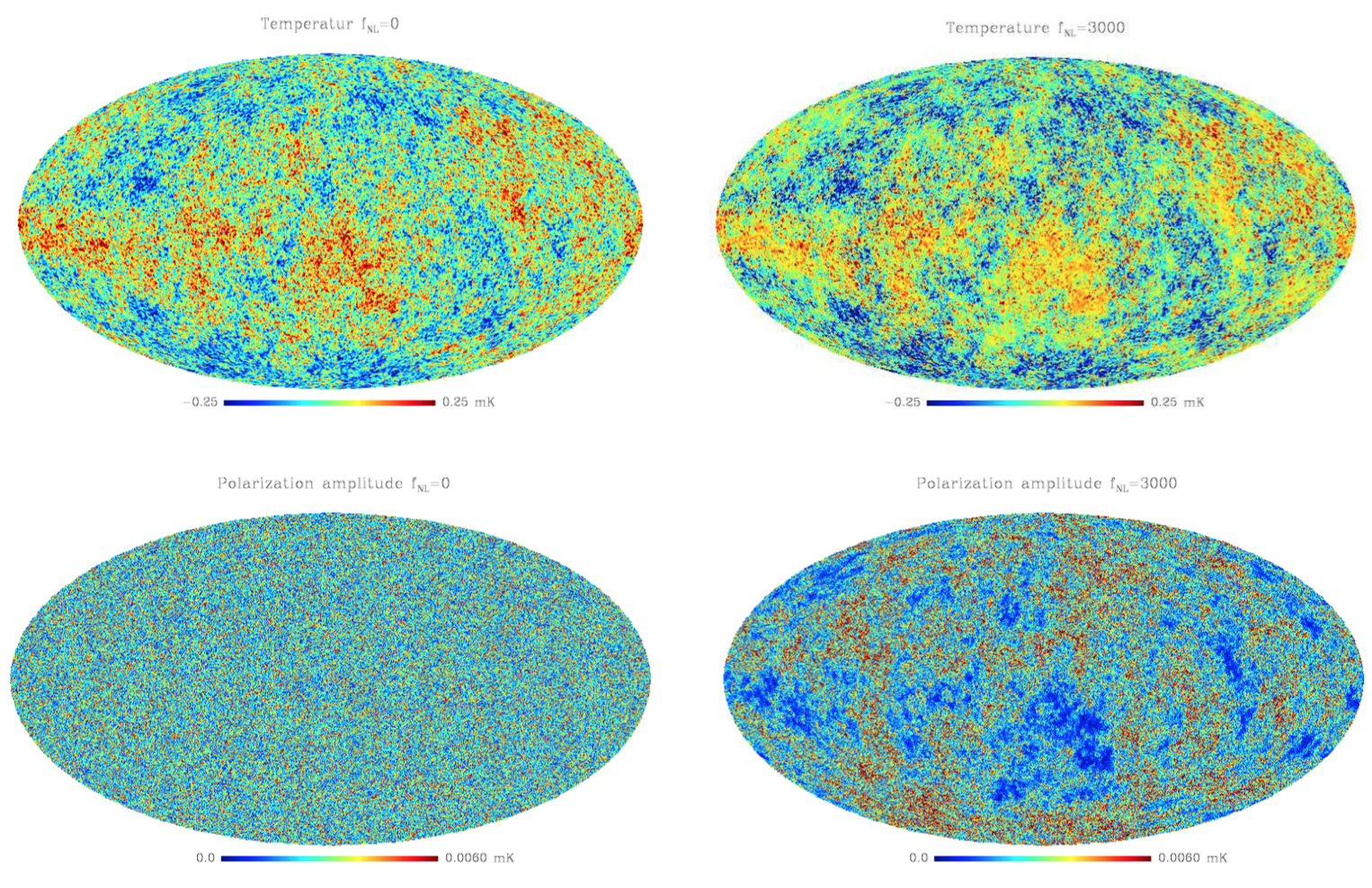
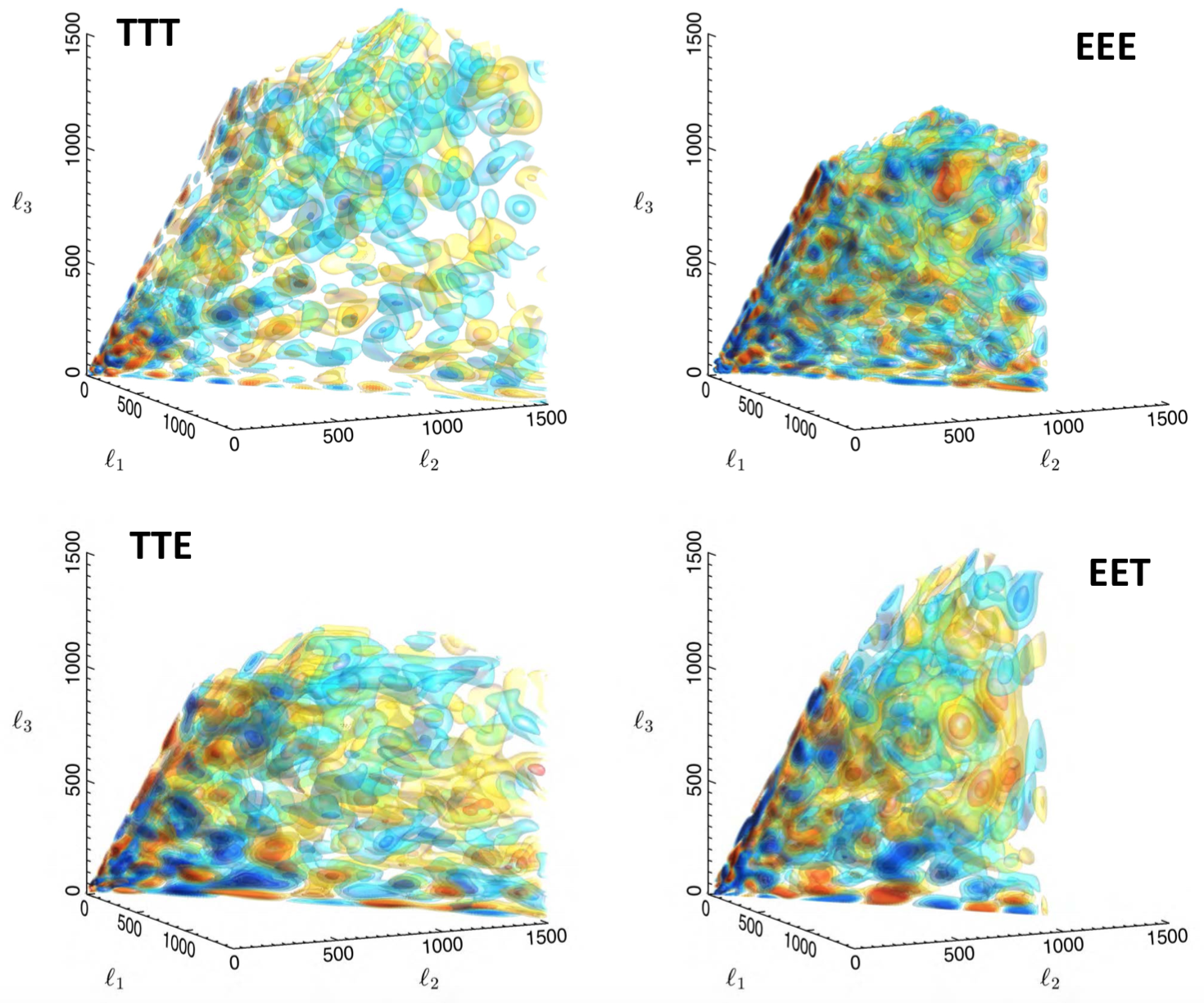
The Planck satellite has measured the CMB temperature and polarization anisotropies with great accuracy, and, since PNG affects both, we can compare the data with the NG CMB simulated maps, shown in Figure 6.

The latest release regarding non-Gaussianity [27] tested the local, equilateral, orthogonal (and many more) shapes for the bispectrum and provided new constraints on the primordial trispectrum parameter $g_{\rm NL}$ (while $\tau_{\rm NL}$ was constrained in the previous release [26]). A new Planck legacy release, which will improve the 2015 results in terms of more refined treatment of $E$-mode polarization, is in preparation.

The standard representation used in the Planck analysis for the CMB bispectrum is

$$B^{m_{1}m_{2}m_{3}}_{\ell_{1}\ell_{2}\ell_{3}}\equiv\left<a_{\ell_{1}m_{1}}a_{\ell_{2}m_{2}}a_{\ell_{3}m_{3}}\right>=\mathcal{G}_{m_{1}m_{2}m_{3}}^{\ell_{1}\ell_{2}\ell_{3}}b_{\ell_{1}\ell_{2}\ell_{3}}$$ (13)

where $\mathcal{G}_{m_{1}m_{2}m_{3}}^{\ell_{1}\ell_{2}\ell_{3}}$ are the Gaunt integrals

$$\mathcal{G}_{m_{1}m_{2}m_{3}}^{\ell_{1}\ell_{2}\ell_{3}}\equiv\int Y_{\ell_{1}m_{1}}(\hat{\mathbf{n}})Y_{\ell_{2}m_{2}}(\hat{\mathbf{n}})Y_{\ell_{3}m_{3}}(\hat{\mathbf{n}})d^{2}\hat{\mathbf{n}}=h_{\ell_{1}\ell_{2}\ell_{3}}\begin{pmatrix}\ell_{1}&\ell_{2}&\ell_{3}\\ m_{1}&m_{2}&m_{3}\end{pmatrix}$$ (14)

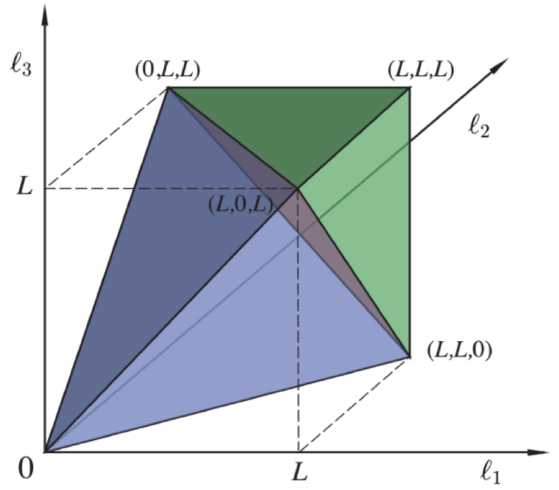
and the $\ell_{j}$ satisfy the following conditions, see Figure 7:

• triangle condition: $\ell_{1}\leq\ell_{2}+\ell_{3}$ for $\ell_{1}\geq\ell_{2},\ell_{3}$ and permutations

• parity condition: $\ell_{1}+\ell_{2}+\ell_{3}=2\ n$ with $n\in\mathbb{N}$

• resolution: $\ell_{1},\ell_{2},\ell_{3}\leq\ell_{max}$ with $\ell_{1},\ell_{2},\ell_{3}\in\mathbb{N}$.

Figure 7: Permitted observational domain for the CMB bispectrum $b_{\ell_{1}\ell_{2}\ell_{3}}$. Allowed multipole values $(\ell_{1},\ell_{2},\ell_{3})$ lie inside the shaded “tetrapyd” region (tetrahedron+pyramid), satisfying both the triangle condition and the experimental resolution. From [26].

As noticed before, the search for PNG is optimized in terms of $f_{\rm NL}$. Leaving aside complications coming from breaking of statistical isotropy (sky-cut, noise, etc.), the general procedure is to fit the theoretical bispectrum template

$$\hat{f}_{\rm NL}=\frac{1}{N}\sum B^{m_{1}m_{2}m_{3}}_{\ell_{1}\ell_{2}\ell_{3}}\left[\left(C^{-1}a\right)^{m_{1}}_{\ell_{1}}\left(C^{-1}a\right)^{m_{2}}_{\ell_{2}}\left(C^{-1}a\right)^{m_{3}}_{\ell_{3}}-3C^{-1}_{\ell_{1}m_{1}\ell_{2}m_{2}}\left(C^{-1}a\right)^{m_{3}}_{\ell_{3}}\right]$$ (15)

to the 3-point function obtained analyzing the data. Unfortunately, a brute force implementation scales like $\ell_{max}^{5}$, unfeasible at Planck (or WMAP) resolution. On the other hand, we can achieve a massive speed improvement ($\ell_{max}^{3}$ scaling) if the reduced bispectrum is separable. Generally, there are different ways to write the theoretical template in separable form:

• the KSW [46] separable template fitting and the Skew-Cl extension [47];

• the binned bispectrum presented in [48];

• the modal expansion described in [49].

The alternative implementations differ basically in terms of the separation technique adopted and of the projection domain.

More recent improvements can be found in [50] where the interested reader can find an exact expression for the multi-variate joint probability distribution function (PDF) of non-Gaussian fields, primordially arising from local transformations of a Gaussian field. This expression has been applied to the non-Gaussianity estimation from CMB maps and the halo mass function, obtaining both analytical expressions as well as approximations with specified range of validity.
The results for the CMB gave a fast way to compute the PDF, valid up to more than $7\,\sigma$ for $f_{\rm NL}$ values not ruled out by current observations, expressed as a combination of bispectrum and trispectrum of the temperature maps. Note that such expression is valid for any kind of non-Gaussianity and is not limited to the local type, providing a useful basis for a fully Bayesian analysis of the NG parameter.

Finally, note that, in principle, we could go to higher order. In fact, this may become important if we want to detect NG in observables characterized by a large $f_{\rm NL}$ (e.g. in high-redshift probes) and/or if $f_{\rm NL}$ (leading order bispectrum) and $g_{\rm NL}$ (leading-order trispectrum) are both depending on the same underlying physical coupling constant that we aim at determining. However, the expressions are rather involved and we refer the reader to [50] for details.

3.1 Planck results on primordial non-Gaussianity

In this section, we briefly present some of the Planck results on PNG, focusing on the improvements compared to the 2013 release and the differences between the methods used in the analysis, particularly concerning the Integrated Sachs-Wolfe (ISW) effect.

Let us start with the 2015 Planck analysis for the bispectrum in the modal representation, described in Figure 8, for the various combinations $TTT$, $EEE$, $TTE$, $EET$.
Note that compared to Planck 2013 the new constraints on local, equilateral, orthogonal bispectra have improved by up to 15%.

Figure 8: CMB temperature and polarization bispectrum reconstructions for Planck SMICA maps using the full set of polynomial modes with $n_{max}=2001$ and with signal-to-noise weighting. From [27].

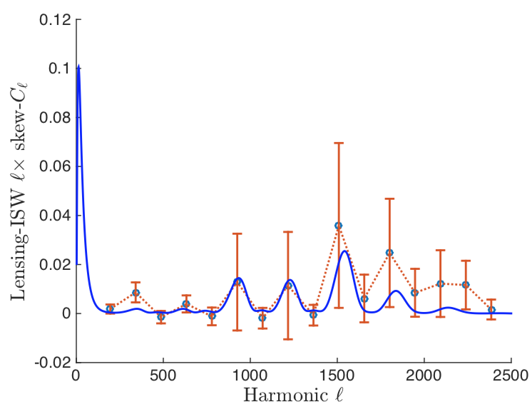
In the 2015 analysis particular attention was devoted to investigate the ISW-lensing effect which strongly affects the constraints on $f_{\rm NL}$ from Planck bispectrum. The results are confirmed using several $f_{\rm NL}$ estimators and CMB maps. Actually, different maps have been produced by the SMICA, NILC, SEVEM  and Commander-Ruler (or C-R) pipelines. Notice that the SMICA product is considered the preferred one overall. Having said this, the amplitude of the ISW-lensing bispectrum from the SMICA, NILC, SEVEM, and C-R  foreground-cleaned maps, for the KSW, binned, and modal (polynomial) estimators are summarized in Table 1. Remarkably, the coupling between weak lensing and ISW effect is the leading contamination to local NG, as the ISW lensing bispectrum has been detected with a significance of $2.8\,\sigma$ (see Figure 9), and improves to $3.0\,\sigma$ when including polarization. In conclusion, the bias in the three primordial $f_{\rm NL}$ parameters due to the ISW-lensing signal is described in Table 2.

lensing-ISW amplitude

Method . SMICA SEVEM NILC Commander

T

KSW . 0.79 $$\pm$$ 0.28 0.78 0.28 0.78 0.28 0.84 0.28

Binned . 0.59 0.33 0.60 0.33 0.68 0.33 0.65 0.36

Modal2 . 0.72 0.26 0.73 0.26 0.73 0.26 0.78 0.27

T+E

Binned . 0.82 0.27 0.75 0.28 0.85 0.26 0.84 0.27

Table 1: Results for the amplitude of the lensing-ISW bispectrum from the SMICA, SEVEM, NILC, and Commander foreground-cleaned maps, for different bispectrum estimators. Error bars are 68 % CL. From [27].

Figure 9: The skew-Cl spectrum for the lensing-ISW effect (red line with data points), from the temperature map. The blue curve is the theoretically-expected spectrum. From [27].

Actually, the new analysis was the first adopting also polarization data for PNG, and the Planck 2015 constraints on $T+E$ have confirmed $T$ results with significantly reduced error bars, see Table 3 for the latest constraints on $f_{\rm NL}$ for the various shapes.
Specifically, the Planck 2013 hints of NG in oscillatory feature models remain in $T$, but decrease significantly when polarization is included. Also, new estimators for high-frequency oscillations cover 10 times more parameter space, compared to the previous analysis.

lensing-ISW $$f_{\rm NL}$$ bias

Shape . SMICA SEVEM NILC Commander

T Local . 7.5 7.5 7.3 7.0

T Equilateral . 1.1 1.2 1.3 1.8

T Orthogonal . 27 27 26 26

E Local . 1.0 1.1 1.0 1.1

E Equilateral . 2.6 2.7 2.5 2.9

E Orthogonal . 1.3 1.3 1.2 1.5

T+E Local . 5.2 5.5 5.1 4.9

T+E Equilateral . 3.4 3.4 3.4 3.6

T+E Orthogonal . 10 11 10 10

Table 2: Bias in the three primordial $f_{\rm NL}$ parameters due to the lensing-ISW signal for the four component separation methods. From [27].

$$f_{\rm NL}$$(KSW)

Shape and method . Independent ISW-lensing subtracted

SMICA   (T)

Local. 10.25.7 2.55.7

Equilateral. 1370 1670

Orthogonal. 5633 3433

SMICA  (T+E)

Local. 6.55.0 0.85.0

Equilateral. 343 443

Orthogonal. 3621 2621

Table 3: Results for the $f_{\rm NL}$ parameters of the primordial local, equilateral, and orthogonal shapes, determined by the KSW estimator from the SMICA foreground-cleaned map. Error bars are $68\,\%$ CL. From [27].

Remarkably, the improvements in the Planck 2015 results have allowed to put new constraints on:

• isocurvature NG, where polarizartion data were crucial in this respect;

• tensor NG, where parity-odd $T$ limits are consistent with WMAP (null result);

• trispectrum due to cubic NG (in particular $g_{\rm NL}$ for a variety of shapes).

Finally, with the 2015 release we could also constraint the three fundamental shapes of the trispectrum

$$g_{\rm NL}^{local} =(-9.0\pm 7.7)\times 10^{4}\,,$$ (16)

$$g_{\rm NL}^{\dot{\sigma}^{4}} =(-0.2\pm 1.7)\times 10^{6}\,,$$

$$g_{\rm NL}^{(\partial{\sigma})^{4}} =(-0.1\pm 3.8)\times 10^{5}\,.$$

In conclusion, the Planck 2015 release contains a largely extended analysis of NG templates, and we expect that the upcoming release (the “Planck legacy” paper) will further improve the constraints on standard shapes (owing to refined treatment of $E$-mode polarization maps) and add some extra shapes (such as scale-dependent $f_{\rm NL}$, conformal symmetry), looking for features both in the power spectrum and the bispectrum.

3.2 Implications for inflation

One of the most important consequence from Planck data is that the simplest inflationary models (standard inflation) are still alive … and in very good shape!
Specifically, for standard inflation we refer to a single scalar field $\phi$ (representing a single clock), characterized by a Bunch-Davies initial vacuum state and a canonical kinetic term $X=-\frac{1}{2}\partial_{\mu}\phi\,\partial^{\mu}\phi$, performing a slow-roll dynamics by means of a potential $\mathcal{V}(\phi)$, minimally coupled to gravity, described by general relativity (GR)

$$S=\int d^{4}x\sqrt{-g}\left[X-\mathcal{V}(\phi)+\mathcal{L}_{int}(\phi,A_{\mu},\Psi)+\frac{M_{Pl}^{2}}{2}\,R\right]$$ (17)

where $\mathcal{L}_{int}$ is the interaction term between the inflaton and other fields such as gauge bosons $A_{\mu}$ or fermions $\Psi$.
Actually, standard inflation predicts tiny ($\mathcal{O}(10^{-2})$, thus no presently detectable) PNG.

However, alternatives to standard inflation have also been considered. In particular, results from Planck 2015 (which increased the number of modes from 600 to 2000 with respect to Planck 2013) constrained $f_{\rm NL}$ for a large number of inflationary models including:

• the equilateral family (DBI, EFT, ghost and K-inflation);

• the flattened shapes (non-Bunch Davies);

• feature models (oscillatory or scale-dependent bispectra);

• direction dependence;

• quasi-single-field;

• parity-odd models.

Since no evidence for NG has been found, we could only put tighter constraints on the parameters from the models above, for example on:

• the curvaton decay fraction $r_{D}>19\%$ (from local $f_{\rm NL}$, $T+E$),

• the speed of sound in the Effective Field Theory of Inflation [51] $c_{S}>0.024$ (from equilateral and orthogonal $f_{\rm NL}$),

• the speed of sound in DBI inflation $c_{S}>0.087$ (from $T+E$).

3.3 Primordial non-Gaussianity with CMB spectral distorsions

Possible measurements to improve the constraints on PNG include CMB spectral distorsions from acoustic wave dissipation that can probe a large range of scales, much more than CMB/LSS [52].

Actually, if $\mu$-anisotropies were measured we would access to

• $T\mu$ correlations, useful to investigate the primordial local $f_{\rm NL}$ (see [53]) or other squeezed shapes, e.g. excited initial states [54],

• $\mu\mu$ correlations, associated to the primordial local trispectrum, $\tau_{\rm NL}$ [55],

• $TT\mu$ bispectrum, related to the primordial local trispectrum $g_{\rm NL}$ [55].

While for Gaussian initial conditions the dissipated power in small patches (from $\approx 50\ \text{Mpc}^{-1}$ to $\approx 10^{4}\ \text{Mpc}^{-1}$) is isotropically distributed, squeezed bispectra associated to local NG generate couplings between large and small scales.
As a consequence of these coupling between long and short modes, the CMB temperature fluctuations on large scales can be coupled to spectral distortions arising from acoustic wave dissipation at very small scales, resulting in $T\mu$ correlations [56, 53, 57].
More specifically, following [57], consider the curvature perturbation at position $\vec{x}$ in terms of a Gaussian random variable $z(\vec{x})$

$$\zeta(\vec{x})=z(\vec{x})+\frac{3}{5}f^{loc}_{\rm NL}z^{2}(\vec{x})\,.$$ (18)

Splitting $\zeta(\vec{x})$ in long-wavelength and short-wavelength modes as $\zeta(\vec{x})=\zeta_{L}(\vec{x})+\zeta_{S}(\vec{x})$, and similarly writing $z(\vec{x})=z_{L}(\vec{x})+z_{S}(\vec{x})$ we get

$$\zeta_{L}+\zeta_{S}=z_{L}+z_{S}+\frac{3}{5}f^{loc}_{\rm NL}[z_{L}^{2}+2\,z_{L}\,z_{S}+z_{S}^{2}]\,,$$ (19)

and we conclude that, in presence of $f_{\rm NL}^{loc}\neq 0$, long and short modes can be coupled. In particular, to linear order in $f_{\rm NL}^{loc}$, the small-scale curvature fluctuation in the presence of some fixed long-wavelength curvature fluctuation is

$$\zeta_{S}=z_{S}\left(1+\frac{6}{5}f^{loc}_{\rm NL}\zeta_{L}\right)$$ (20)

thus modulating the (fractional) chemical-potential fluctuation, given by [56, 57, 58]

$$\frac{\delta\mu}{\mu}\approx\frac{\delta\left<\zeta^{2}\right>}{\left<\zeta^{2}\right>}\approx\frac{12}{5}f^{loc}_{\rm NL}\zeta_{L}\,.$$ (21)

Similarly, for the large-angle ($\ell\lesssim 100$, probing causally disconnected regions at the last scattering surface) the temperature fluctuation is determined primarily by the curvature fluctuation at the surface of last scatter, given by $\delta T/T\approx\zeta/5$ [56, 57].
As a consequence, the fractional chemical potential fluctuation $\frac{\delta\mu}{\mu}$ and the temperature fluctuation $\frac{\delta T}{T}$ are cross correlated with an angular power spectrum $C_{\ell}^{\mu T}$ equal to [56, 57]

$$C_{\ell}^{\mu T}=12f^{loc}_{\rm NL}C_{\ell}^{TT}\,.$$ (22)

4 Primordial non-Gaussianity and the Large-Scale Structure

Non-Gaussianity in Large-Scale Structure can be either of primordial origin or associated to gravitational instability.
In particular, to make contact with the CMB definition, PNG in LSS can be defined starting from the DM density fluctuation $\delta$ through the Poisson’s equation

$$\delta=-\left(\frac{3}{2}\Omega_{m}H^{2}\right)^{-1}\nabla^{2}\Phi$$ (23)

where we have used the comoving gauge for density fluctuation [59].
As before, we can write

$$\Phi=\phi_{L}+f_{\rm NL}(\phi_{L}^{2}-\left<\phi_{L}^{2}\right>)+g_{\rm NL}(\phi^{3}-\left<\phi_{L}^{2}\right>\phi_{L})+\dots$$ (24)

where $\phi_{L}$ is the linear Gaussian contribution and $f_{\rm NL}$ and $g_{\rm NL}$ are dimensionless non-linearity parameters .

In order to investigate PNG in LSS, generally N-body simulations have been playing a crucial role [60, 61, 62, 63, 64, 65, 66, 67]. The standard equations are

$$\Phi =\phi_{L}+f_{\rm NL}(\phi_{L}^{2}-\left<\phi_{L}^{2}\right>)$$ (25)

$$\nabla^{2}(\Phi\ast T)g(z) =-4\pi Ga^{2}\delta\rho_{DM}$$

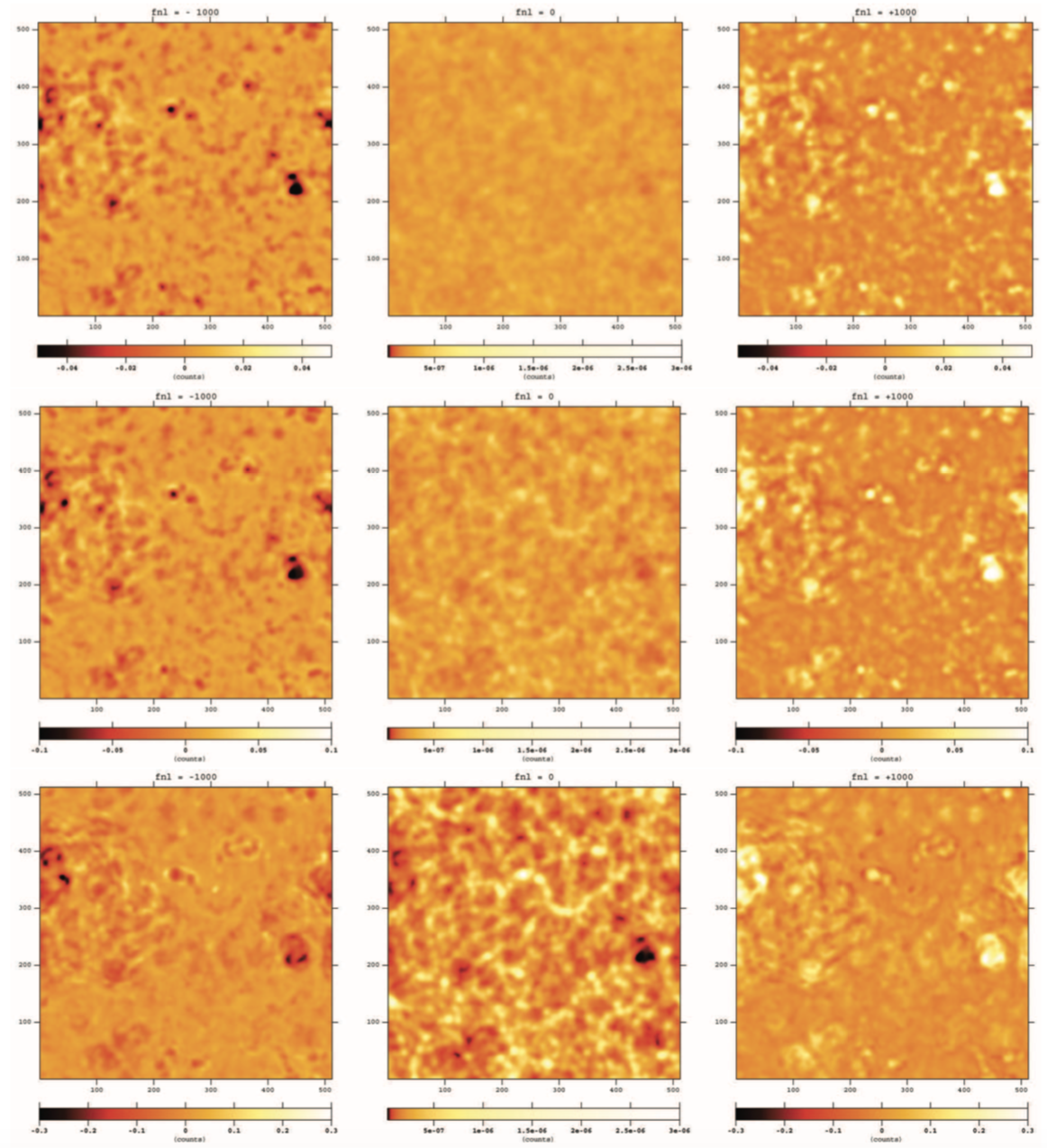
where $T$ is the matter transfer function and $g$ is the growth suppression factor. Typical results are shown in Figure 10.

Figure 10: Slice maps of simulated mass density fields at $z=5.15$ (top), $z=2.13$ (middle) and $z=0$ (bottom). The number of pixels at a side length is $512$ ($500h^{-1}$ Mpc) and that of the thickness is $32$ ($31.25h^{-1}$ Mpc). The panels in the middle row show the log of the projected density smoothed with a Gaussian filter of $10$ pixels width, corresponding to $9.8h^{-1}$ Mpc. The left and right panels are the relative residuals for the $f_{\rm NL}=\pm 1000$ runs. Each panel has the corresponding color bar and the range considered are different from panel to panel. From [61].

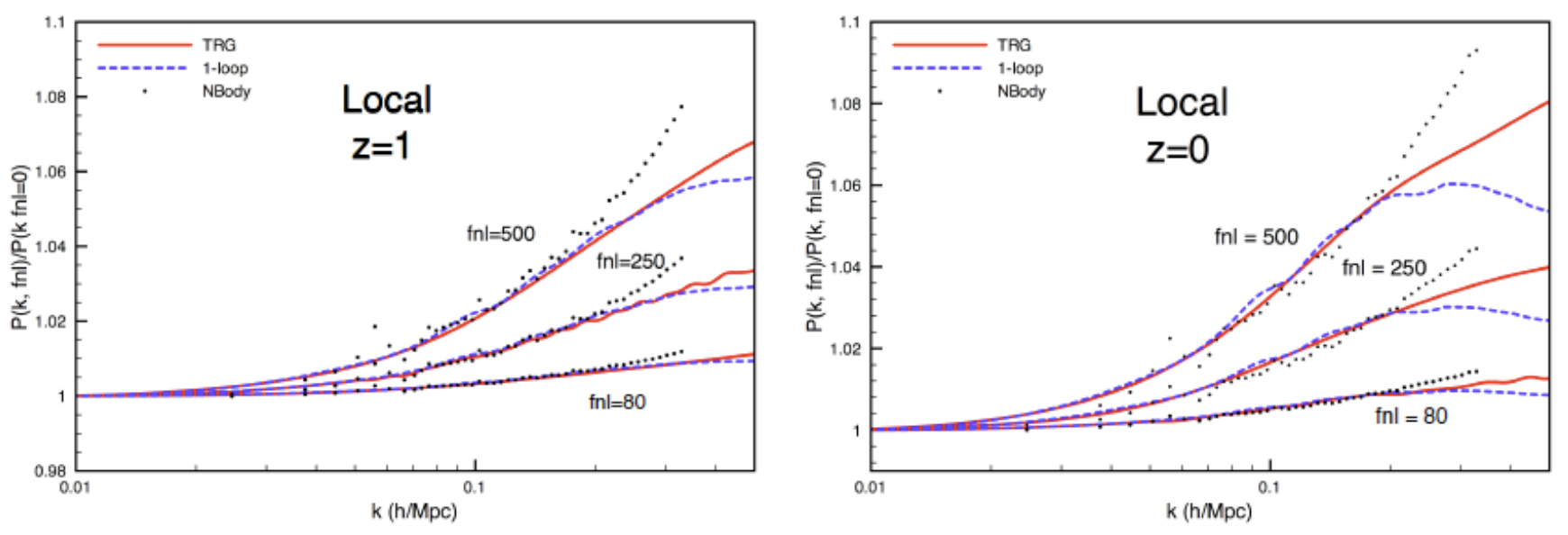
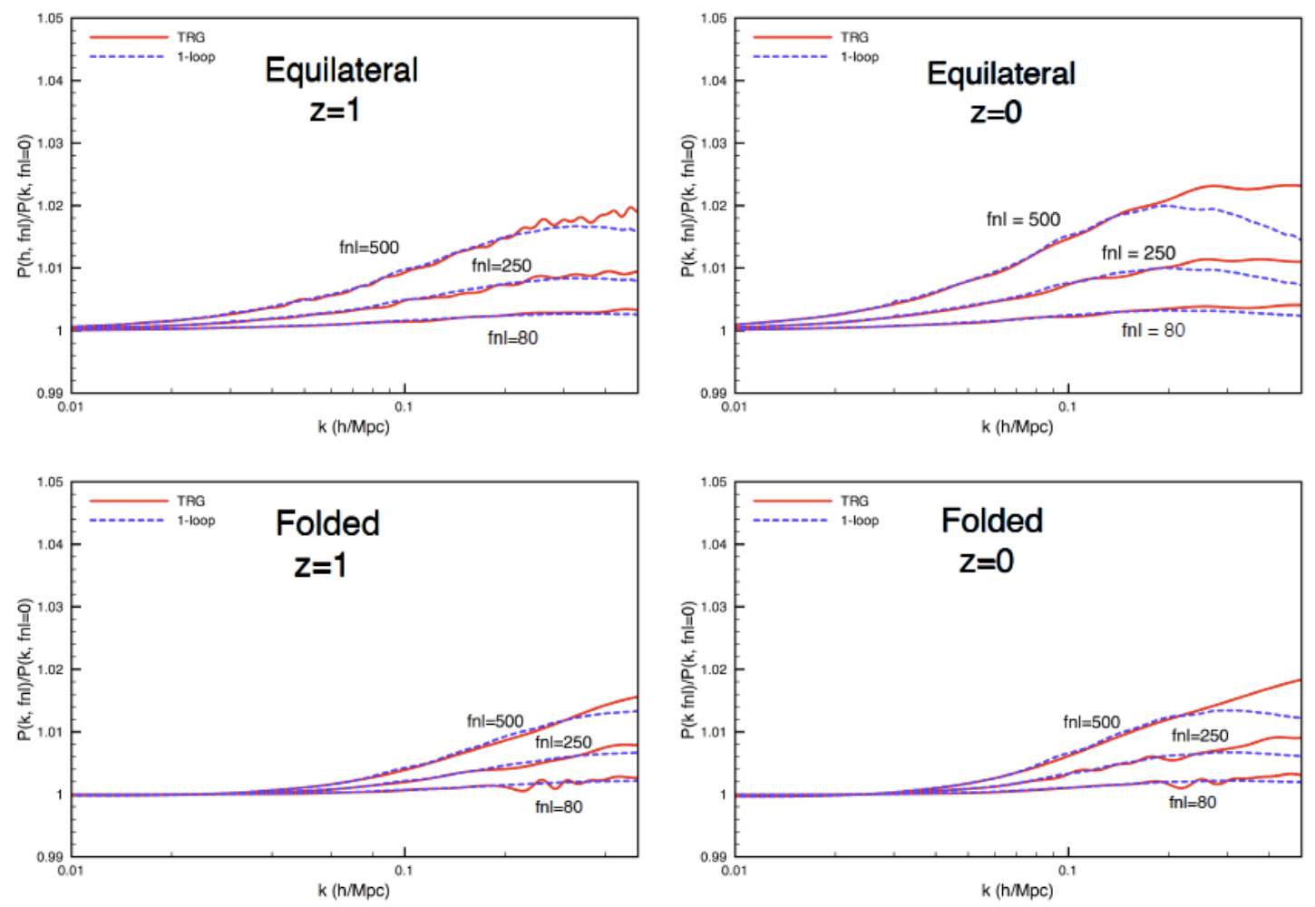
However, in the mild non-linear regime, analytical approaches have been developed to study the PNG effects on the matter power spectrum. Results for the local shape calculated using the Time Renormalization Group theory [68, 69] compared to N-body are shown in Figure 11, while for the equilateral and folded shapes see Figure 12.
Similar techniques include the renormalized perturbation theory [70, 71, 72], renormalization group approach [73], closure theory [74], Lagrangian perturbation theory [75, 76, 77], the time-sliced perturbation theory [78] and the Effective Field Theory of LSS (EFTofLSS) [79, 80]. Specifically, the EFTofLSS for non-Gaussian initial conditions have been developed in [81], see also [82, 83, 84, 85, 86, 87, 88].

Figure 11: Ratio of the non-Gaussian to Gaussian power spectrum for several values of $f_{\rm NL}$ in the local model. The dots correspond to the data from the N-body simulations of [89]. The red (continuous) line is the TRG result of this paper and the blue (dashed) line is the one-loop result. From [90].

Figure 12: Ratio of the non-Gaussian to Gaussian power spectrum for several values of $f_{\rm NL}$ in the equilateral (top panels) and folded (bottom panels) models. The red (continuous) lines are the TRG result of this paper and the blue (dashed) lines are the one-loop result. From [90].

4.1 Non-Gaussianity and halo mass function

Besides using the standard statistical estimators, like the (mass) bispectrum, trispectrum, etc., one can look at the tails of the distribution, i.e. at rare events.

Rare events have the advantage that they often maximize deviations from what is predicted by a Gaussian distribution, but have the obvious disadvantage of being rare! But remember that, according to the Press-Schechter-like schemes, all collapsed DM halos correspond to (rare) high peaks of the underlying density field.

In [91, 92] it was shown that clusters at high redshift ($z>1$) can probe NG down to $f_{\rm NL}\sim 10^{2}$, see also [93] for an alternative approach. Actually, many methods have been developed for the determination of mass function, such as

• the stochastic approach (first-crossing of a diffusive barrier) [94, 95, 96, 97],

• the ellipsoidal collapse method [98, 99],

• a combination of saddle-point and diffusive barrier [100],

• the Log-Edgeworth expantion [101],

• the excursion sets studied with correlated steps [102, 103].

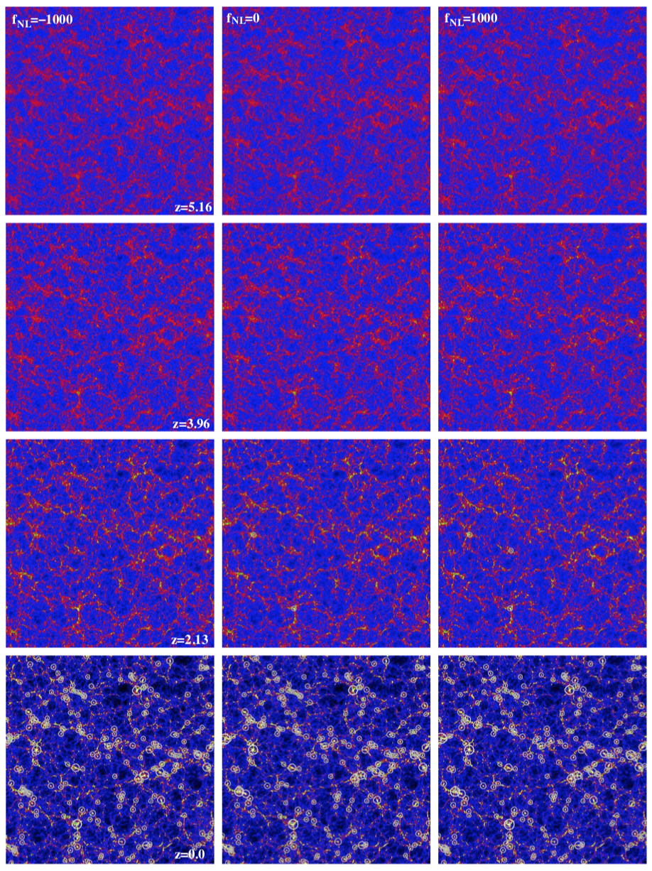
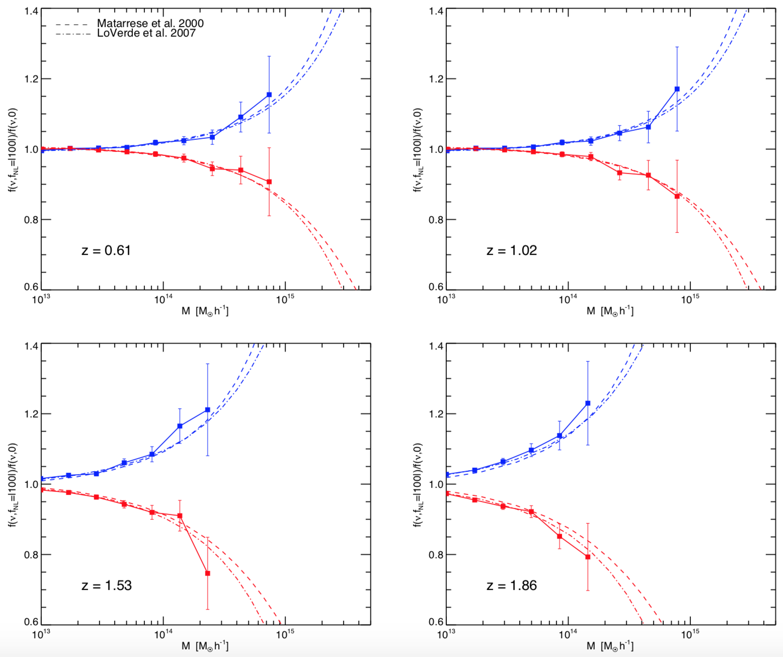
Remarkably, excellent agreement of analytical formulae with N-body simulations (e.g. see Figure 13 for DM halos in NG simulations and Figure 14 for the ration of the non-Gaussian $f_{\rm NL}$ to Gaussian mass function) have been found in [89, 64, 62], and in many other papers afterwards e.g. [104, 105, 106].

Figure 13: Mass density distribution and halo positions in a slice cut across the simulation box. The color-coded contours indicate different density levels ranging from dark (deep blue) underdense regions to bright (yellow) high density peaks. The halo positions are indicated by open circles with size proportional to their masses. Left panels: NG model with $f_{\rm NL}=-1000$. Central panels: Gaussian model. Right panels NG model with $f_{\rm NL}=+1000$. The mass and halo distributions are shown at various epochs, characterized by increasing redshifts (from bottom to top), as indicated in the panels. From [60].

Figure 14: Ratio of the non-Gaussian ($f_{\rm NL}=\pm 100$) to Gaussian mass function for different redshift snapshots: top left $z=0.61$; top right $z=1.02$; bottom left $z=1.53$; bottom right $z=1.86$. The dashed line is the mass function of [92] and the dot-dashed lines are that of [93], both including the $q$-correction. From [64].

Moreover, halo (galaxy) clustering and halo (galaxy) higher-order correlation functions represent further and more powerful implementations of this general idea.
Actually, the halo mass function (à-la-Press-Schechter) can be a useful tool to probe PNG as it essentially depends exponentially on the PNG parameters [92], by modulating the critical overdensity for collapse. Its calculation can be done along the lines of the original Press-Schechter approach, using a steepest-descent approximation to deal with (small) PNG. However, several effects have to be carefully considered such as non-Markovianity, already there in the Gaussian case, but unavoidable in NG case, or the details of the non-spherical collapse. While analytical treatments are welcome, the validation with N-body simulations is crucial. Still we need to better understand the connection between analytical and numerical quantities and real observables, and to what level is this affecting NG measurements.

• Should we necessarily go on with (extended) Press-Schechter-like approaches?

• Are alternative approaches viable such as Smoluchowski equation for the non-Poissonian random process (or the earliest attempt proposed in [107])?

In conclusion, rare events (e.g. high-z and massive clusters) offer interesting and promising opportunities for the detection of PNG, as both the mass-function of massive haloes and the number-counts of massive haloes are affected.

4.2 Halo bias in NG models

As it is well known, halos (galaxies) do not trace the underlying (dark) matter distribution. For this reason, following the original proposal [108], we introduce the “bias” parameters or Eulerian bias for galaxy clusters and later for galaxies (for a review see [109])

$$\delta_{halo}(x)=b_{1}\delta_{matter}(x)+b_{2}\delta_{matter}^{2}(x)+\dots$$ (26)

that allow to parametrize our ignorance about the way in which dark matter halos cluster in space with respect to the underlying dark matter.
Note that a complete set of the local bias terms (representing all possible local gravitational observables along the fluid trajectory) was presented in [110, 111, 112]. For the most general expansion up to second order in the Eulerian framework with Gaussian initial condition see also [113, 114, 115, 116, 117, 118, 119, 120, 121]. The various bias parameters can be generally regarded either as purely phenomenological ones (i.e. to be fitted to observations) or predicted by a theory (e.g. Press-Schecter together with Lagrangian perturbation theory).
Specifically, considering $\delta_{halo}(x)=b\ \delta_{matter}(x)$, it is possible to show that the halo bias is sensitive to PNG through a scale-dependent correction term (in Fourier space), see e.g. [122, 19, 123, 124, 125, 126, 127, 128, 129]. In particular, we have

$$\frac{\delta b(k)}{b}\sim\frac{2f_{\rm NL}\delta_{c}}{k^{2}}\,.$$ (27)

This opens interesting prospects for constraining or measuring NG in LSS but demands for an accurate evaluation of the effects of (general) NG on halo biasing.

The idea is to start from the results obtained in the 80’s in [130, 131] giving the general expression for the peak 2-point function as a function of N-point connected correlation functions of the background linear (i.e. Lagrangian) mass-density field

$$\xi_{h,M}(|\mathbf{x}_{1}-\mathbf{x}_{2}|)=-1+\exp\left\{\sum_{N=2}^{\infty}\sum_{n=1}^{N-1}\frac{\nu^{N}\sigma_{R}^{-N}}{j!(N-1)!}\xi^{(N)}\left[\underset{\text{$j$ times}}{\mathbf{x}_{1},\dots,\mathbf{x}_{1}},\underset{\text{$(N-j)$ times}}{\mathbf{x}_{2},\dots,\mathbf{x}_{2}}\right]\right\}$$ (28)

which requires many techniques such as the path-integral, the cluster expansion, the multinomial theorem and asymptotic expansion. The analysis of NG models was motivated in [132] on bulk flows.

In [123] this relation was applied to the case of NG of the gravitational potential, obtaining the power-spectrum of dark matter halos modeled as high “peaks” (up-crossing regions) of height $v=\delta_{c}/\sigma_{R}$ of the underlying mass density field (Kaiser’s model). Here $\delta_{c}(z)$ is the critical overdensity for collapse (at redshift $z$) and $\sigma_{R}$ is the root mean square mass fluctuation on scale $R$ ($M\sim R^{3}$).

The motion of peaks (going from Lagrangian to Eulerian space), which implies [116]

$$1+\delta_{h}(\mathbf{x}_{Eulerian})=(1+\delta_{h}(\mathbf{x}_{Lagrangian}))(1+\delta_{R}(\mathbf{x}_{Eulerian}))$$ (29)

and (to linear order) $b=1+b_{L}$ [133], allows to derive the scale-dependent halo bias in the presence of NG initial conditions. Corrections may arise from second-order bias and GR terms.

Alternative approaches (e.g. based on 1-loop calculations) have been developed in [74, 134, 76, 135]. Improvements in the fit with N-body simulations by assuming dependence on gravitational potential have been carried out in [63], while for the extension to bispectrum see [136]. Finally, the inclusion of $g_{\rm NL}$ and $f_{\rm NL}$ in analysis of QSO clustering was performed in [25].
Note that the extension to general (scale and configuration dependent) NG is straightforward [123]. Actually, we can write, in full generality, the $f$ bispectrum as $B_{f}(k_{1},k_{2},k_{3})$. Then, the relative NG correction to the halo bias is

$$\frac{\Delta b_{h}}{b_{h}}= \frac{\Delta_{c}(z)}{D(z)}\frac{1}{8\pi^{2}\sigma_{R}^{2}}\int dk_{1}\,k_{1}^{2}\mathcal{M}_{R}(k_{1})\times$$ (30)

$$\int_{-1}^{1}d\mu\frac{\mathcal{M}_{R}(\sqrt{\alpha})}{\mathcal{M}_{R}(k)}\frac{B_{\phi}(k_{1},\sqrt{\alpha},k)}{P_{\phi}(k)}$$

where $\alpha=k_{1}^{2}+k_{2}^{2}+2k_{1}k\mu$, $P_{\phi}$ is the power-spectrum of a Gaussian gravitational potential, while $\mathcal{M}_{R}$ is the factor connecting the smoothed linear overdensity with the primordial potential by means of the factor

$$\mathcal{M}_{R}(k)=\frac{2}{3}\frac{T(k)k^{2}}{H_{0}^{2}\Omega_{m,0}}W_{R}(k)$$ (31)

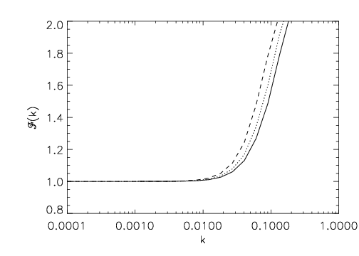
where $T(k)$ is the transfer function and $W_{R}(k)$ is the window function defining the radius $R$ of a proto-halo of mass $M(R)$. It also applies to non-local (e.g. “equilateral”) PNG (corresponding to DBI or ghost inflation) and universal PNG term (see also [126, 137, 138, 139]). The halo bias in NG models has been calculated in [123], the result is

$$b_{h}^{f_{\rm NL}}=1+\frac{\Delta_{c}(z)}{\sigma_{R}^{2}D^{2}(z)}\left[1+2f_{\rm NL}\frac{\Delta_{c}(z)}{D(z)}\frac{\mathcal{F}_{R}(z)}{\mathcal{M}_{R}(z)}\right]$$ (32)

where the form factor is given by

$$\mathcal{F}_{R}(k)=\frac{1}{8\pi^{2}\sigma_{R}^{2}}\int dk_{1}k_{1}^{2}\mathcal{M}_{R}(k_{1})P_{\phi}(k_{1})\int_{-1}^{1}d\mu\mathcal{M}_{R}(\sqrt{\alpha})\left[\frac{P_{\phi}(\sqrt{\alpha)}}{P_{\phi}(k)}+2\right]$$ (33)

and plotted, for three different masses, in Figure 15.

Figure 15: The function $\mathcal{F}_{R}(k)$ for three different masses: $1\times 10^{14}M_{\odot}$ (solid), $2\times 10^{14}M_{\odot}$ (dotted), $1\times 10^{14}M_{\odot}$ (dashed). From [123].

4.3 PNG with LSS: the galaxy bispectrum

The bispectrum of galaxies can be used to forecast the constraining power of LSS surveys on measuring the amplitude of PNG, see e.g. [140, 141]. In this section, we derive, following [142], the galaxy bispectrum.
The starting point is the relation between the linearly evolving density field $\delta_{lin}$ and the primordial gravitational potential

$$\delta_{lin}(\mathbf{k},z)=\alpha(k,z)\Phi_{in}(\mathbf{k})$$ (34)

with $\alpha(k,z)$ defined as

$$\alpha(k,z)\equiv\frac{2k^{2}c^{2}T(k)D(z)}{3\Omega_{m}H_{0}^{2}}$$ (35)

where $T(k)$ is the transfer function. Since the linearly evolving density includes non-Gaussian terms in presence of PNG, we can define the Gaussian part as

$$\delta_{G}(\mathbf{k},z)=\alpha(k,z)\varphi_{G}(\mathbf{k})\,.$$ (36)

With this definition, using second-order (Eulerian) perturbation theory, we get [143]

$$\delta^{(2)}(\mathbf{k},z) =\int\frac{d\mathbf{k}_{1}}{(2\pi)^{3}}\int\frac{d\mathbf{k}_{2}}{(2\pi)^{3}}\delta^{D}(\mathbf{k}-\mathbf{k}_{1}-\mathbf{k}_{2})\times$$ (37)

$$\times\left[\mathcal{F}_{2}(\mathbf{k}_{1},\mathbf{k}_{2})+f_{\rm NL}\frac{\alpha(k)}{\alpha(k_{1})\alpha(k_{2})}\right]\delta_{G}(\mathbf{k}_{1},z)\delta_{G}(\mathbf{k}_{2},z)$$

where the 2-nd order gravity-kernel $\mathcal{F}_{2}$ is given by

$$\mathcal{F}_{2}(\mathbf{k}_{1},\mathbf{k}_{2})=\frac{5}{7}+\frac{1}{2}\frac{\mathbf{k}_{1}\cdot\mathbf{k}_{2}}{k_{1}k_{2}}\left(\frac{k_{1}}{k_{2}}+\frac{k_{2}}{k_{1}}\right)+\frac{2}{7}\frac{(\mathbf{k}_{1}\cdot\mathbf{k}_{2})^{2}}{k_{1}^{2}k_{2}^{2}}\,.$$ (38)

The quantity $\delta(x)$ is expressed in the Eulerian frame, with the initial spatial coordinate $\mathbf{q}$ in the Lagrangian frame being related to the evolved Eulerian coordiate $\mathbf{x}$ through the formula

$$\mathbf{x}(\mathbf{q},\tau)=\mathbf{q}+\mathbf{\Psi}(\mathbf{q},\tau)$$ (39)

where $\mathbf{\Psi}$ is the displacement field. Using this relation, we can rewrite the second-order solution appearing in (37) as [144, 145]

$$\delta^{(2)}(\mathbf{x},\tau)=\frac{17}{21}(\delta_{lin}(\mathbf{x},z))^{2}+\frac{2}{7}s^{2}(\mathbf{x},z)-\mathbf{\Psi}(\mathbf{x},z)\cdot\nabla\delta(\mathbf{x},z)$$ (40)

where $s^{2}=s_{ij}s^{ij}$ and $s_{ij}$ is the trace-free tidal tensor, defined as

$$s_{ij}\equiv\left(\nabla_{i}\nabla_{j}-\frac{1}{3}\delta_{ij}^{K}\nabla^{2})\nabla^{-2}\delta\right)$$ (41)

and $\delta_{ij}^{K}$ is the Kronecker delta. In the following, we will omit the redshift dependence in the density and velocity fields.

We can introduce a long-short splitting of the gravitational potential and DM density field, such that, for local NG one easily finds (for local NG)

$$\delta_{lin,\ell}(\mathbf{k})=\delta_{G,\ell}+f_{\rm NL}\alpha(\varphi_{G,\ell}^{2}-\left<\varphi_{G,\ell}^{2}\right>)$$ (42)

with

$$\varphi_{G}(\mathbf{q})=\varphi_{G,\ell}(\mathbf{q})+\varphi_{G,s}(\mathbf{q})\,.$$ (43)

In Lagrangian space one can then introduce the expansion

$$\delta_{g}^{L}(\mathbf{q}) =\frac{n_{g}(\mathbf{q})-\left<n_{g}\right>}{\left<n_{h}\right>}$$ (44)

$$=b_{10}^{L}\delta_{lin}+b_{01}^{L}\varphi_{G}+b_{20}^{L}(\delta_{lin})^{2}+b_{11}^{L}\delta_{lin}\varphi_{G}+b_{02}^{L}\varphi_{G}^{2}+\dots$$

where the $5$ $b_{ij}$ represent our (generally unknown) bias parameters.
The final Eulerian position of the galaxy can be obtained by using the conservation law [116]

$$1+\delta_{g}^{E}(\mathbf{x},z)=[1+\delta(\mathbf{x},z)][1+\delta_{g}^{L}(\mathbf{q},z)]$$ (45)

to find

$$\delta_{g}^{E}(\mathbf{k})=\delta_{10}^{E}\delta+b_{01}^{E}\varphi_{G}+b_{20}^{E}\delta\ast\delta+b_{11}^{E}\delta\ast\varphi_{G}+b_{02}^{E}\varphi_{G}\ast\varphi_{G}-\frac{2}{7}b_{10}^{L}s^{2}-b_{01}n^{2}$$ (46)

where $s^{2}$ and $n^{2}$ are suitable expansion terms and the Eulerian bias parameters read:

$$b_{10}^{E} =1+b_{10}^{L}\,,$$ (47)

$$b_{01}^{E} =b_{01}^{L}\,,$$

$$b_{20}^{E} =\frac{8}{21}b_{10}^{L}+b_{20}^{L}\,,$$

$$b_{11}^{E} =b_{01}^{L}+b_{11}^{L}\,,$$

$$b_{20}^{E} =b_{02}^{L}\,.$$

Using the standard definitions for the galaxy power spectrum $P_{gg}$ and bispectrum $B_{ggg}$

$$\left<\delta_{g}^{E}(\mathbf{k}_{1})\delta_{g}^{E}(\mathbf{k}_{2})\right> =(2\pi)^{3}\delta^{D}(\mathbf{k}_{1}+\mathbf{k}_{2})P_{gg}(\mathbf{k}_{1})\,,$$ (48)

$$\left<\delta_{g}^{E}(\mathbf{k}_{1})\delta_{g}^{E}(\mathbf{k}_{2})\delta_{g}^{E}(\mathbf{k}_{3})\right> =(2\pi)^{3}\delta^{D}(\mathbf{k}_{1}+\mathbf{k}_{2}+\mathbf{k}_{3})B_{ggg}(\mathbf{k}_{1},\mathbf{k}_{2},\mathbf{k}_{3})\,.$$

we can simply write at tree-level

$$P_{gg}(\mathbf{k}_{1}) =E_{1}^{2}(\mathbf{k}_{1})P(k_{1})$$ (49)

$$B_{ggg}(\mathbf{k}_{1},\mathbf{k}_{2},\mathbf{k}_{3}) =2E_{1}(\mathbf{k}_{1})E_{1}(\mathbf{k}_{2})E_{2}(\mathbf{k}_{1},\mathbf{k}_{2})P(k_{1})P(k_{2})+2\ \text{cyc.}$$

where $P(k)$ is the matter power spectrum for the Gaussian source field $\varphi_{G}$, while the kernels $E_{i}$ are defined as

$$E_{1}(\mathbf{k}_{1})=b_{10}+\frac{b_{01}}{\alpha(k_{1})}$$ (50)

with the scale dependent bias term $b_{01}/\alpha(k_{1})\propto f_{\rm NL}/k_{1}^{2}$, and

$$E_{2}(\mathbf{k}_{1},\mathbf{k}_{2})= \ b_{10}\left[F_{2}(\mathbf{k}_{1},\mathbf{k}_{2})+f_{\rm NL}\frac{\alpha(|\mathbf{k}_{1}+\mathbf{k}_{2}|)}{\alpha(k_{1})\alpha(k_{2})}\right]$$ (51)

$$+\left[b_{20}-\frac{2}{7}b_{10}^{L}S_{2}(\mathbf{k}_{1},\mathbf{k}_{2})\right]+\frac{b_{11}}{2}\left[\frac{1}{\alpha(k_{1})}+\frac{1}{\alpha(k_{2})}\right]$$

$$+\frac{b_{02}}{\alpha(k_{1})\alpha(k_{2})}-b_{01}\left[\frac{N_{2}(\mathbf{k}_{1},\mathbf{k}_{2})}{\alpha(k_{2})}+\frac{N_{2}(\mathbf{k}_{2},\mathbf{k}_{a})}{\alpha(k_{1})}\right]\,.$$

Note that, general relativistic effects (including also redshift-space distortions, lensing, etc.) have to be taken into account both in the galaxy power-spectrum and bispectrum, as well as in the dark matter evolution.
The complete expression (very involved) for the galaxy bispectrum was written down for the first time recently, and can be found in [146] to be soon compared with observations, see also [147, 148, 149].

We conclude this section describing, following [142], the Fisher matrix forecasts on $\sigma_{f_{\rm NL}}$ (the accuracy of the determination of local non-linear parameter $f_{\rm NL}$) from measurements of the galaxy bispectrum, as well as the constraints on PNG from the galaxy power spectrum and bispectrum in future radio continuum and optical surveys [150]. See also [151] for the constraining power on primordial non-Gaussianity of the Dark Energy Survey (DES) as well as Euclid and WFIRST.
Particularly, the tree-level bispectra with local non-Gaussian initial conditions are shown in Table 4 in redshift space, where the covariance between different triangles has been neglected.
While many issues are still present (such as the need for full covariance, a better understanding of accurate bias model, the inclusion of general relativistic effects, or the proper implementation of the estimators), still moving from the 2D Planck data to the 3D maps of the forthcoming surveys represent a great potential as

• the bispectrum could do better than the power-spectrum,

• we might increase the accuracy to achieve $f_{\rm NL}\sim 1$.

In particular, the LSS bispectrum allows in principle tight constraints also on non-local shapes (e.g. equilateral). However, even if naive mode counting suggest that $\sigma_{f_{\rm NL}}\sim 1$ for the equilateral shape might be achievable by pushing $k_{max}$ high enough, modeling the gravitational bispectrum in the non-linear regime with high accuracy is very challenging, as the equilateral shape is more correlated than local to the non-linear gravitational bispectrum.

	Power Spectrum		Bispectrum
Sample	$\sigma_{f_{\rm NL}}$	$\sigma_{f_{\rm NL}}$	$\sigma_{f_{\rm NL}}$	$\sigma_{f_{\rm NL}}$
	bias float	bias fixed	bias float	bias fixed
BOSS	$21.30$	$13.28$	$1.04^{(0.65)}_{(2.47)}$	$0.57^{(0.35)}_{(1.48)}$
eBOSS	$14.21$	$11.12$	$1.18^{(0.82)}_{(2.02)}$	$0.70^{(0.48)}_{(1.29)}$
Euclid	$6.00$	$4.71$	$0.45^{(0.18)}_{(0.71)}$	$0.32^{(0.12)}_{(0.35)}$
DESI	$5.43$	$4.37$	$0.31^{(0.17)}_{(0.48)}$	$0.21^{(0.12)}_{(0.37)}$
BOSS + Euclid	$5.64$	$4.44$	$0.39^{(0.17)}_{(0.59)}$	$0.28^{(0.11)}_{(0.34)}$

Table 4: Forecasts for $\sigma_{f_{\rm NL}}$, the accuracy of the determination of local $f_{\rm NL}$, from the bispectrum of BOSS, eBOSS, DESI and Euclid. From [142].

Finally, possible future constraints on the amplitude $f_{\rm NL}$ for the local, equilateral and orthogonal shapes, through galaxy power spectrum and bispectrum measurements on large scales based on radio continuum (with 10 $\mu$Jy and 1 $\mu$Jy flux limits) and optical (spectroscopic and photometric) surveys are presented in Table 5, see [150] for details. Remarkably, for the local shape, LSS measurements can provide significant improvements over current Planck constraints on PNG.

	Planck	1 $\mu$Jy	10 $\mu$Jy	Spectroscopic	Photometric
Local	5.0	0.2	0.6	1.3	0.3
Equilateral	43	244	274	57	184
Orthogonal	21	18	29	18	38

Table 5: Summary of $1\sigma$ limits for the three PNG types considered, from radio continuum and optical surveys derived from combining the power spectrum and bispectrum and accounting for RSD, the trispectrum term and theoretical errors. From [150].

5 Controversial issues on non-Gaussianity

In this section, we present some aspects regarding non-Gaussianity which we think are still controversial or require further clarifications.

5.1 Single-field consistency relation

The first issue concerns the single-field consistency relation. Actually, as mentioned before, the common lore is that the “consistency relation”, implying $f_{\rm NL}=-5\,(n_{s}-1)/12$, can be gauged away by a non-linear rescaling of coordinates, up to sub-leading terms. As a consequence, the only residual term is proportional to $\epsilon$ thus of the same order of the amplitude of tensor modes.
More precisely, the bispectrum for single-field inflation can be represented as [6, 10, 11]:

$$B_{\zeta}(k_{1},k_{2},k_{3}) \propto\frac{(\Delta_{\zeta}^{2})^{2}}{(k_{1}k_{2}k_{3})^{2}}\left[(1-n_{s})\mathcal{S}_{loc.}(k_{1},k_{2},k_{3})+\frac{5}{3}\epsilon\mathcal{S}_{equil.}(k_{1},k_{2},k_{3})\right]$$ (52)

$$n_{s} =1-\eta-2\epsilon\,,\quad\text{with}\quad\epsilon\equiv\frac{\dot{H}}{H^{2}}\,,\ \eta\equiv\frac{\dot{\epsilon}}{H\epsilon}\,.$$

The observability of the so-called “Maldacena consistency relation”, related to the above bispectrum for single field inflation, in CMB and LSS data, has led to a long-standing controversy.
Recently, various groups have argued that the $(1-n_{s})$ term is totally unobservable (for single-clock inflation), as, in the strictly squeezed limit (one of the wave-numbers, say $k_{i}$, going to 0, $k_{i}\rightarrow 0$), this term can be gauged away by a suitable coordinate tranformation.
However, in [152] it has been argued that the term survives up to a “renormalization” which further reduces it by a factor of $\sim 0.1$ if one applies Conformal Fermi Coordinates (CFC) to get rid of such a “gauge mode”.

• Is this (CFC approach) the only way to deal with this term?

• Can we aim at an exact description, which is not affected by “spurious PNG”?

5.2 Non-Gaussian $f_{\rm NL}$-like terms generated by non-linear general relativistic evolution

An other important issue regards the role of the non-linear evolution of the matter perturbations in general relativity. Actually, second order DM dynamics in GR leads to (post-Newtonian) $\delta\zeta$-like terms which mimic local primordial non-Gaussianity [153]. For instance, these terms have been included in the halo bias in [125].
For a recent estimate of the effective non-Gaussianity due to general-relativistic lightcone effects mimicking a PNG signal, see [154] .

Remarkably, these GR terms can be recovered by a short-long mode splitting ($\lambda_{S}$ and $\lambda_{L}$, respectively) leading to a resummed non-linear contribution $\delta e^{-2\zeta}$ [157]. This comes from the modulation of sub-horizon scales due to modes entering the horizon at any given time. In the comoving gauge (suitable for calculation of halo bias) this would correspond to an $f_{\rm NL}=-5/3$ in the pure squeezed limit.
Then, we may ask the following question

• is such relativistic NG signature detectable via some cosmological observables?

Consider a patch of the Universe, where the comoving spatial element is given by

$$ds^{2}_{(3)}=e^{2\zeta}\delta_{ij}dx^{i}dx^{j}\,.$$ (53)

There is a global background which must be defined with respect to some scale $\lambda_{0}$, at least as large as all the other scales of interest, i.e., at least as large as our presently observable Universe.
Then, there is an other important scale, the separate Universe patches, $\lambda_{P}$, distinguished from $\lambda_{0}$ and we assume $\lambda_{0}\gg\lambda_{P}\gg\lambda_{S}$. This is large enough for each patch to be treated as locally homogeneous and isotropic, but patches must be stitched together to describe the long-wavelength perturbations on a scale $\lambda_{L}\gg\lambda_{P}$, see Figure 16. Thus,

$$\lambda_{0}>\lambda_{L}\gg\lambda_{P}\gg\lambda_{S}\,.$$ (54)

Figure 16: Schematic of the various scales in Eq. (54). From [158].

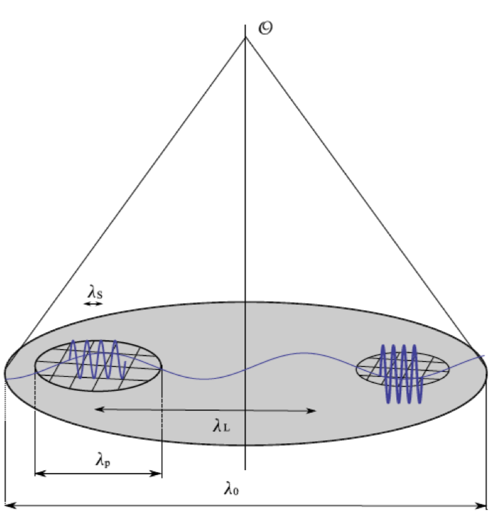
The local observer in a separate Universe patch cannot observe the effect of $\zeta_{L}$, which is locally homogeneous on the patch scale $\lambda_{P}$. However, local coordinates can be defined only locally and the long mode curvature perturbation is observable through a mapping from local to global coordinates.

In the halo bias case the effect is unobservable. Indeed, as pointed out in [159, 160, 161], a local physical redefinition of the mass gauges away such a NG effect (in the pure squeezed limit), similarly to Maldacena’s single-field NG contribution. This is true provided the halo bias definition is strictly local. We may ask the following questions:

• are there significant exceptions?

• are all non-linear GR effects fully accounted for by “projection effects”?

In general, this dynamically generated GR non-linearity is physical and cannot be gauged away by any local mass-rescaling, provided it involves scales larger than the patch required to define halo bias, but smaller than the separation between halos (and the distance of the halo to the observer).
Hence one would expect it to be in principle detectable in the matter bispectrum. Similarly, the observed galaxy bispectrum obtained via a full GR calculation must include all second-order GR non-linearities on such scales (only as projection effects?).

In conclusion, the separate Universe approach is very useful for many applications, but the effect of the external world cannot be always described by linear theory, thus the usual identification of large scales with the linear theory is only qualitative and can become misleading in some cases.
For example, on one hand, perturbations of order $N\gg 1$ give the leading contribution to $N$-th order moments, such as $\left<\delta^{N}\right>_{c}$. On the other hand, we know from non-linear Newtonian dynamics that $\left<\delta^{N}\right>_{c}\sim\left<\delta^{2}\right>^{N-1}$ on all scales (for scale-free spectra). Well inside a given separate Universe, the assumption that the only non-linearity is described by Newtonian physics might be too restrictive, as the relevance of non-linear GR effects in sub-patch dynamics depends upon the specific problem.

It would be interesting to see the effects of using, for example, the silent Universe description ([162]) to account for deviations of the patch from purely spherical behavior. Recall that over-dense patches evolve towards oblate ellipsoids and even under-dense ones can collapse to oblate ellipsoids, owing to tidal effects of surrounding matter. Recent approaches using the local tide approximation [163] go in this direction.

6 Concluding remarks

The concordance $\Lambda$CDM cosmological model describes the evolution of the Universe from 380,000 years after the Big Bang to the present time with astonishingly accuracy. However, the mechanism that generated the primordial fluctuations representing the seeds of the structures we observe in the CMB and in the LSS is unknown. Remarkably, inflation provides a causal mechanism for the generation of cosmological perturbations, whose detailed predictions are fully supported by CMB and LSS data.
Clearly, the direct detection of PGW and PNG with the specific features predicted by inflation would provide strong independent support to this framework.

In the previous sections, we have summarized the theoretical motivations for PNG and the present observational status. As stated before, Planck has provided stringent limits on $f_{\rm NL}$ which will be improved with polarization maps and using the full data in the upcoming “Planck legacy” paper.
In conclusion, among the short term goals, we need to look for more non-Gaussian shapes, such as scale-dependent $f_{\rm NL}$, make use of the bispectrum in 3D data and improve the constraints on $g_{\rm NL}$.

The final goal is to reconstruct the inflationary action by improving the sensitivity on NG parameters, searching for $f_{\rm NL}\sim 1$ for all shapes, taking into account non-linear general relativistic effects and second-order radiation transfer function contributions.