All-sky angular power spectra from cleaned WISESuperCOSMOS galaxy number counts
Abstract
Aiming to extract cosmological information from linear scales of the WISESuperCOSMOS photometric redshift catalog, we perform a characterization of the systematic effects associated with stellar content, evidencing the presence of contamination and obscuration. We create an integrated model for these effects (which together we call “usurper contamination”), devise a method to remove both of them simultaneously and show its functionality by applying it to a set of mock catalogs. When administered to WISESuperCOSMOS data, our method shows to improve the measurements of angular power spectra on scales and the extraction of cosmological parameters therefrom, even though a significant excess of power remains at these scales. When ignoring scales , we still find strong indications of systematics, albeit these can be localized in the southern equatorial hemisphere. An independent analysis of the northern hemisphere at agrees with the CDM model with parameters from the Planck satellite and gives and at 95% confidence limit when combined with priors on , and .
1 Introduction
Galaxy and quasar surveys are key observational tools in cosmology. Through them we can probe the matter distribution in the Universe and, therefore, test predictions of cosmological models and constrain their parameters [1, 2, 3, 4, 5, 6, 7, 8, 9]. A few interesting questions that have been tackled using wide-angle surveys are the homogeneity and isotropy of the Universe [10, 11, 12], the shape of the distribution function of galaxy density [13], the behavior of gravity and the growth of structure [14, 15], the accelerated expansion of the Universe and the properties of dark energy [16, 17], the amount of matter in the Universe [18], the existence of primordial non-Gaussianities [19] and the mass of neutrinos [20, 21].
To improve constraints on the relevant cosmological parameters – especially on the equation of state of dark energy, the mass of neutrinos, and on non-Gaussianities and other inflation signatures – deeper and wider surveys are desirable [22, 23, 24]. Moreover, these surveys are required in order to improve our knowledge in various other interesting topics. For instance, the cross-correlation between galaxy distribution and gravitational lensing of the cosmic microwave background (CMB) – which serves as a consistency check for our cosmological model, besides helping improve constraints on halo bias and on the amplitude of matter perturbations – peaks at large angular scales [25]. This is also the case for the integrated Sachs-Wolfe effect [26], probed by the cross-correlation of CMB temperature maps with galaxy distribution, whose signal comes from the evolution of gravitational potential along the CMB photon path. Another topic that requires almost full-sky galaxy surveys is the measurement of our own peculiar velocity with respect to all other galaxies [27, 28, 29]. Large galaxy surveys can also help us improve our understanding of galaxy bias, that could be enhanced at the largest scales if we assume that galaxies form at density peaks (see e.g. [30]).
This type of studies are among the main aims of the largest forthcoming surveys. The Large Synoptic Survey Telescope222http://www.lsst.org/ (LSST) [31] will cover up to redshifts , while the Euclid space telescope333http://www.euclid-ec.org will observe 15,000 and detect galaxies up to [32]. The huge volume probed by these surveys will lead to such a high number of observed galaxies and quasars that spectroscopic measurements will be performed only for a small fraction of them, while for most sources we will have to rely on photometric redshifts (photo-s hereafter) and photometric classification. These techniques are, however, plagued with high contamination levels, large systematic effects and uncertainties, which must be controlled and understood in order to fully mine the relevant datasets.
An existing testbed for such surveys is the WISESuperCOSMOS catalog [33] (WSC hereafter), a full-sky photometric galaxy dataset reaching . Our goal in this paper is to estimate cosmological parameters from this sample under the standard cosmological model CDM. In this process, we characterize the systematic effects associated with stellar density (which, although more prominent in the WSC, will also be present in LSST and Euclid) and devise a method for mitigating such effects, tested on simulations and real data. These efforts were aimed at improving the survey’s reach toward the largest scales (), commonly distrusted in cosmological analyses (e.g. [34, 35]). Finally, we also verified the impact of different assumptions about photo- properties on the measured parameters.
This work adds to previous WSC analyses that have investigated its observational and cosmological properties, such as hemispherical anisotropies [36], Minkowski functionals [37], cross-correlation with CMB lensing [38, 39] and temperature [40]. It also contributes with a new strategy for mitigating systematics to those previously proposed [41, 42, 43, 44, 45, 46].
The basic technique we employ here – the measurement of angular power spectra in tomographic redshift shells – has been applied before to other photometric galaxy catalogs such as the MegaZ [47] and the 2MASS Photometric Redshift datasets (2MPZ) [34], to photometric quasar samples [42] and spectroscopic galaxy data [35].
The outline of this paper is as follows: in Sec. 2 we describe the datasets used in this work, namely the WSC, the Sloan Digital Sky Survey, and the Gaia Data Release 2 catalogs. In Secs. 3.1 and 3.2 we expose the stellar contamination and obscuration effects existent in WSC. A method of modeling and mitigating these effects is presented in Sec. 3.3. The WSC data had their angular power spectra measured and cosmological parameters inferred using the methodology described in Sec. 4. Using simulations, we validate our treatment of systematic effects and our measurement methodology in Sec. 5. Our results – WSC angular power spectra and inferred cosmological parameters – are shown in Sec. 6. Sec. 7 presents tests for robustness and systematics, and in particular, Sec. 7.7 shows evidence for a systematic effect represented by a tension in the cosmological parameters constrained from the angular clustering measured from different equatorial hemispheres. Finally, we conclude and summarize our work in Sec. 8.
2 The dataset
The main dataset used in this work is the WISESuperCOSMOS (WSC) galaxy catalog [33], described in Sec. 2.1. To estimate the stellar contamination and obscuration in WSC, we used the Sloan Digital Sky Survey (SDSS) [48] and Gaia DR2 [49, 50] photometric catalogs as tracers of stars. These are described in Secs. 2.2 and 2.3, respectively.
2.1 WISESuperCOSMOS
The WSC catalog is a cross-match between two parent full-sky catalogs: the AllWISE release [51] from the Wide-field Infrared Survey Explorer (WISE) [52], a mid-infrared space survey in four bands – (3.4, 4.6, 12 and 22); and the SuperCOSMOS Sky Survey [53], a program of automated digitalization of optical photographic plates in the , and filters, taken by the United Kingdom Schmidt Telescope (UKST, in the southern hemisphere) and the Palomar Observatory Sky Survey-II (POSS-II, in the northern hemisphere).
To build the WSC catalog, only the bands , , and were used. Following the magnitude limits of the parent surveys, all WSC sources have magnitudes , and . To preferentially select galaxies over quasars and stars, WSC only includes extended sources according to SuperCOSMOS morphological classification meanClass. It should be noted that the SuperCOSMOS morphological classification is not as accurate as most recent optical surveys; its angular resolution is approximately [54], and the quality of the imaging technique is lower (photographic plates vs. CCDs).
We also point out that the WSC star/galaxy separation is not based only on SuperCOSMOS morphology but also on WISE colours [33]. WSC sources have (a cut aimed at removing bright stars), and (two color-cuts aimed at removing quasars). In this work, we further enforced: the requirement for all sources to reduce stellar contamination and maintain a constant galaxy selection function across the sky (in opposition to a cut dependent on Galactic latitude [33]); maximum Galactic extinction, ; removal of sources in highly contaminated regions such as near the Galactic plane and bulge, around the Magellanic Clouds and in regions presenting unusually high densities according to a lognormal distribution, all accomplished with the WSC final mask [33]; removal of sources in regions where Gaia stellar density is greater than 7 times its average (this increases the masked region around the bulge; see Sec. 2.3); and removal of a SuperCOSMOS tile with bad photometry.
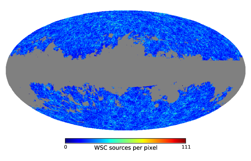
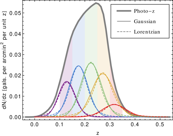
The photo-s for all the WSC sources were obtained with the artificial neural network code ANN [56]444http://www.homepages.ucl.ac.uk/~ucapola/annz.html, trained on a WSC cross-match with the complete and deep Galaxy And Mass Assembly (GAMA)-II spectroscopic dataset [57]. The adequacy of GAMA for photo- training in WSC has been discussed and demonstrated in [33]. As explained there, these photo-s were further corrected for asymmetries between their northern and southern distributions, likely caused by differences between the POSS-II and UKST pass-bands. That paper contains also a comprehensive analysis of photo- properties based on comparisons with several external spectroscopic datasets. A projection of all sources in the photometric redshift (photo-) range is presented in Fig. 1, and Fig. 2 shows the photo- distribution of WSC galaxies. In this work we binned the WSC sources in photo- shells of width , covering the range . However, for reasons presented in Sec. 3, most of our analysis ignores the first bin ().
It was shown in [38] that the WSC photo- errors can be modeled by a Gaussian with zero mean (i.e. no bias) and standard deviation . Also, that an even better model would be a generalized Lorentzian, where the probability density of a galaxy with photo- to have true redshift is:
| (2.1) |
where denotes the Gamma function. The WSC photo-s follows and .
The spectroscopic redshift (spec-) distribution of the galaxies in our photo- bin can be estimated from a convolution of and the photo- distribution :
| (2.2) |
where the th bin in photo- ranges from to . The resulting distributions in the different redshift bins are shown in Fig. 2. We verified that the expected spec- distributions in each bin are very well fitted by a Gaussian (generalized Lorentzian) when the photo- errors are Gaussian (generalized Lorentzian). Also, one can see in Fig. 2 that the mean values of the spec-s in every bin are practically independent of the distribution assumed for the photo- errors, whereas the FWHM may depend on it. Thus, when computing theoretical angular power spectra s to fit the data, we decided to keep the means of the spec- distributions fixed and let the widths vary as nuisance parameters.
2.2 Sloan Digital Sky Survey
The Sloan Digital Sky Survey (SDSS, [48]) is one of the largest astronomical surveys in operation. Here we use its Data Release (DR14) [58]. The survey has already covered of the northern hemisphere, imaging in the five broad bands. The effective photometric limit of the survey is ( completeness for point sources). In addition, its spectroscopic counterpart is complete down to for the Main Galaxy Sample (MGS) and deeper for other sub-projects, such as the Baryon Oscillation Spectroscopic Survey (BOSS) [16].
Despite containing a wealth of cosmological information, the SDSS data was only used here to verify the existence of stellar contamination and obscuration in the WSC catalog, as described in Sec. 3. The SDSS star-galaxy separation classifies extended objects as galaxies and those point-like as stars. This classification is based on a difference between two types of magnitudes, namely sources with are classified as galaxies and otherwise as stars.555The two types of magnitudes and represent magnitudes obtained using the point spread function (PSF) model and the best linear combination of exponential and de Vaucouleurs profiles, respectively. Note that the ‘stars’ according to this definition will include any point sources, also extragalactic ones such as quasars. The PSF of arcsec (full width at half maximum, FWHM) allows for a reliable star-galaxy separation up to [59] and accurate astrometric positions ( arcsec per coordinate) at [60].
2.3 Gaia
Gaia is a space mission of the European Space Agency (ESA) aimed at measuring the three-dimensional positions and velocities of about Milky Way stars [49]. It uses two optical telescopes of collecting area equipped with astrometry, photometry and spectrometry instruments. The astrometry is performed in the range nm (-band hereafter). Gaia Data Release 2 (DR2, [50]) contains point sources with measured parallaxes and proper motions at milliarcsecond (mas) and mas per year () precision, respectively, up to a band magnitude of 20.
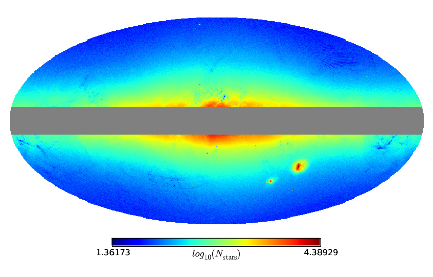
In order to create a representative full-sky stellar density map using the Gaia DR2 source catalog, we had to ensure minimal observational effects (i.e. anisotropic completeness) and minimal contamination by galaxies and quasars. To achieve the first goal we applied a magnitude cut ; as the limiting magnitudes in the regions of interest (away from the Galactic plane) are [61], we expect uniform sky completeness under this selection criterion. The second goal was achieved by taking advantage of the excellent astrometric measurements of Gaia: we assumed that the majority of observed stars should have either a non-zero parallax or a non-zero total proper motion. Thus, we enforced, for all the selected sources, a 5 detection of at least one of these quantities. We computed the total proper motion as , where , is the proper motion in the direction of right ascension and is the proper motion in the direction of declination . The uncertainty on was computed with the usual error propagation, taking into account the covariance between and measurement errors.
In order to avoid regions of high stellar density, here we only selected sources at Galactic latitudes . A map of the selected Gaia sources, in Galactic coordinates, is presented in Fig. 3.
3 Characterizing and cleaning the WSC catalog
3.1 Stellar contamination
As described in [33], the WSC catalog is affected by considerable stellar contamination, especially near the Galactic plane. In order to demonstrate this contamination, we follow the strategy applied in [33] of cross-matching WSC with SDSS photometric sources, taking advantage of the latter’s better star-galaxy separation. Our final analysis, however, is based on a stellar density template derived from Gaia’s observations (see Sec. 3.3).
We cross-matched the WSC sample and the photometric SDSS DR14, linking the nearest objects in the latter (within 2 arcsec) to objects in the former. In total, our cross-matched sample consists of sources which includes both stars and galaxies. The result of this cross-match is shown in Fig. 4. From the bottom panel, it is quite clear that stellar contamination exists and increases towards the Galactic plane and bulge. Also, there are hints that the WSC galaxies are partly obscured by stars, since the top panel shows a deficit of galaxies in the same regions where stars creep in. Overall, 96% percent of the matched sources are galaxies and 4% are stars, according to SDSS.
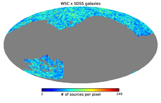
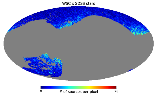
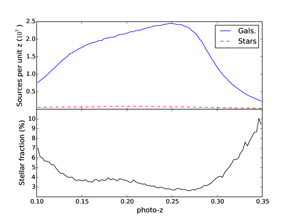
Fig. 5 shows how the amount of stellar contamination changes with redshift. We can see that, at high redshifts, the contamination (i.e. stellar fraction) increases significantly. This increase (and the one at low redshift) are mostly caused by a drop in the number of observed galaxies and not by an increase in the number of misclassified stars (see the top panel).
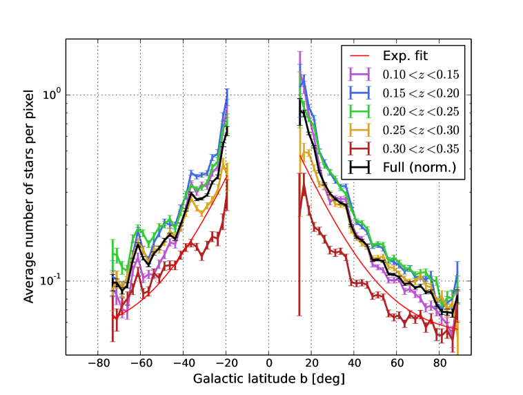
The average dependence with Galactic latitude of the number of stars contaminating WSC (according to SDSS classification) is shown in Fig. 6. We see that both Galactic hemispheres, as well as different redshift ranges, follow very similar trends. For instance, the binned redshift curves differ from the full range one mostly by a constant factor. Despite these similarities, subtle slope changes and hemispherical asymmetries are noticeable.
Figure 6 also shows the result of an exponential fit to the average number of stars per pixel in the range as a function of Galactic latitude :
| (3.1) |
where , and ; in the plot, the fit was scaled by 0.71 to ease visualization. We can see that the fit represents the stellar density reasonably well.
3.2 Stellar obscuration
As shown in Fig. 4 and already noted in previous works with SDSS data [41], the density of observed galaxies anti-correlates with the stellar density: regions with high concentration of stars tend to present lower galaxy counts. We call this phenomenon stellar obscuration. This is expected to affect mostly photometric datasets, such as WSC, due to issues such as blending and source misidentification. Spectroscopic surveys can avoid stellar contamination given that spectroscopy can easily separate stars from galaxies, but even they suffer from such obscuration, as shown in [41].
The approach used in [41] to estimate stellar obscuration was to correlate the observed number of galaxies with the density of foreground stars: as galaxies are, on average, homogeneously distributed on the sky, these two should be uncorrelated in the absence of systematic effects. This approach is feasible in the spectroscopic SDSS case because the galaxy sample there is free from stellar contamination. For WSC sources that include a large amount of stars disguised as galaxies, however, this approach is not possible: correlating WSC sources with stellar density would mix contributions from obscuration and contamination.
An alternative approach is to look at the standard deviation of the counts of galaxies inside pixels as a function of stellar density. The basic idea is that stellar obscuration will not only modulate the mean observed density but also the cosmological fluctuations around the mean, since the former multiplies the latter. Let us formalize this statement through a model for the observed projected density of sources at angular position , for a particular redshift bin , that takes into account both contamination and obscuration:
| (3.2) |
In the equation above, is the survey binary window function, is a template for the expected density of stars, is the real galaxy density, and and are Poisson fluctuations in the number of observed galaxies and stars, respectively. The non-negative parameters and control the amount of obscuration and contamination in the th bin, respectively. The noise terms obey the statistical properties , , and , such that the variance of the total noise is equal to the expected number of observed sources, .
Our model for the observed sources (Eq. 3.2) makes three important simplifications: first, the number of observed galaxies is linearly suppressed by the stellar density; second, both contamination and obscuration depend on the same template; third, the template is independent of redshift, although the final obscuration and contamination are modulated by bin-dependent parameters and . The fact that both obscuration and contamination follow the same template leads to a replacement of galaxies for stars, and thus we call this combined effect “usurper contamination”.
To estimate from the observed variance of , we first write as a pair of generalized coordinates , where specifies an isocontour of while by varying we move along this isocontour. We then compute the mean of for a fixed :
| (3.3) |
where
| (3.4) |
and
| (3.5) |
Note that due to our choice of coordinates, the value of only depends on . Also, we assumed that when averaging the noise along , we may approximate the result to zero. Now we can define the difference and compute the variance of source number counts for an isocontour of :
| (3.6) |
where is the true galaxy variance (i.e. it does not include systematic effects nor shot-noise). Eq. (3.6) assumes that the mean source number counts in , , approximates the expected value , and that is independent of the angular position. By placing all directly measurable quantities on the left hand side, we get a function of that might be fitted to extract the obscuration parameter :
| (3.7) |
In the absence of obscuration, the quantity on the left would be the variance due to cosmological fluctuations (and thus we call it ) and it should be constant all over the sky. We point out that, in practice, the estimation of is performed in a discrete way [the integral in Eq. (3.6), for instance, is actually a sum over pixels], and the isocontours are approximated by bands of similar values.
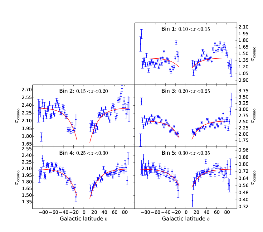
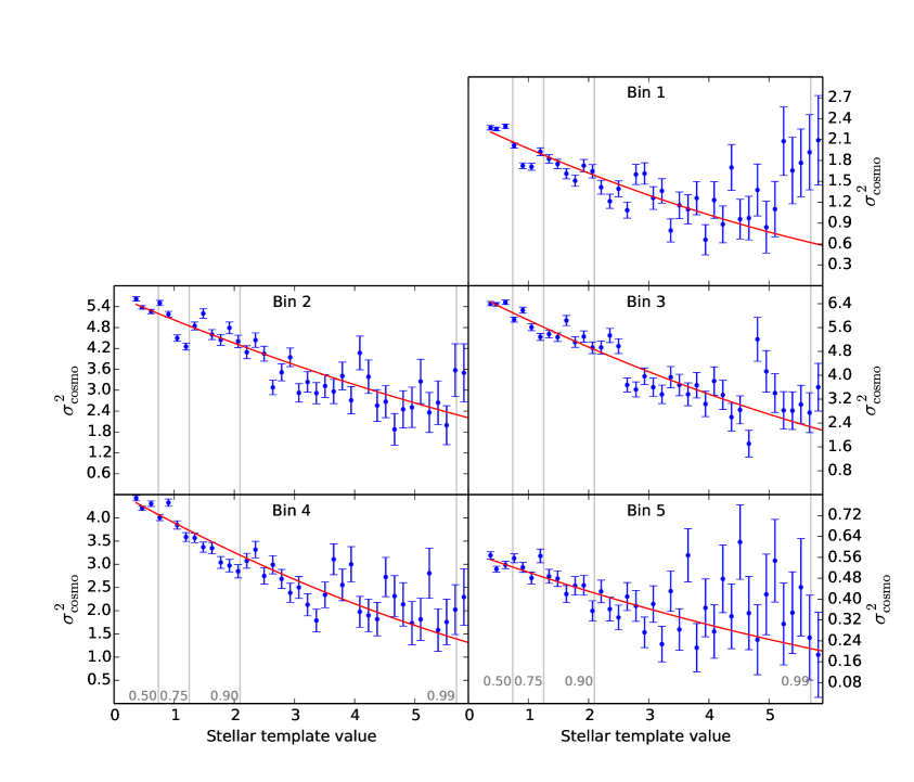
Fig. 7 shows as a function of Galactic latitude for each photo- bin. It is completely evident that the amplitude of the observed fluctuations is not constant and decreases towards the Galactic plane, quantitatively proving the existence of obscuration in the WSC data. This figure also shows that our obscuration model, given by the square root of Eq. (3.7) (depicted as a red line) describes really well the overall behavior of this effect (except for the first bin). Here it is important to emphasize that only and were fitted to , while was held fixed according to Eq. (3.1), estimated from contamination. Thus, Fig. 7 also shows that our assumption that both obscuration and contamination follow the same template is reasonable.
The error bars in Fig. 7 were computed by error propagation from the uncertainties on and , which are given by and , respectively [ is the number of pixels taken into account in each isocontour]. We interpret the fact that the scatter of the data points is larger than the one expected from the error bars as an indication that actually varies from one isocontour to another due to large-scale density fluctuations that are the size of the isocontours. It might also indicate that other factors are in play (e.g. Galactic extinction, seeing and bad photographic plates) or that the template can be improved.
3.3 Cleaning the WSC projected galaxy distribution
We can note from Fig. 6 that the stellar contamination is not perfectly symmetric across the Galactic plane. Moreover, Fig. 3 shows that the stellar density (and likely contamination) is larger near the Galactic bulge, as expected. Aiming at improving the removal of contamination and obscuration from WSC projected galaxy distribution, we built a stellar density template from the Gaia DR2 map presented in Fig. 3, which should accurately represent the stellar distribution – and thus contamination and obscuration – all over the sky.
A few unusually bright pixels – with excessive object counts due to the presence of globular clusters and nearby dwarf galaxies – can be seen in Fig. 3. To remove these count peaks, we computed, for all the pixels, the median of the number counts in neighboring pixels; if the central pixel value was more than twice the median, we replaced the former by the latter. Then, to attenuate the Poisson noise (visible in Fig. 6), we applied Gaussian smoothing with standard deviation arcmin in order to retain all the structure in our template up to the scales of interest. Finally, we applied the same mask as in the data (see Sec. 2.1) and normalized the template by its mean value (the template’s absolute scale does not affect the data treatment). The final result is shown in Fig. 8.
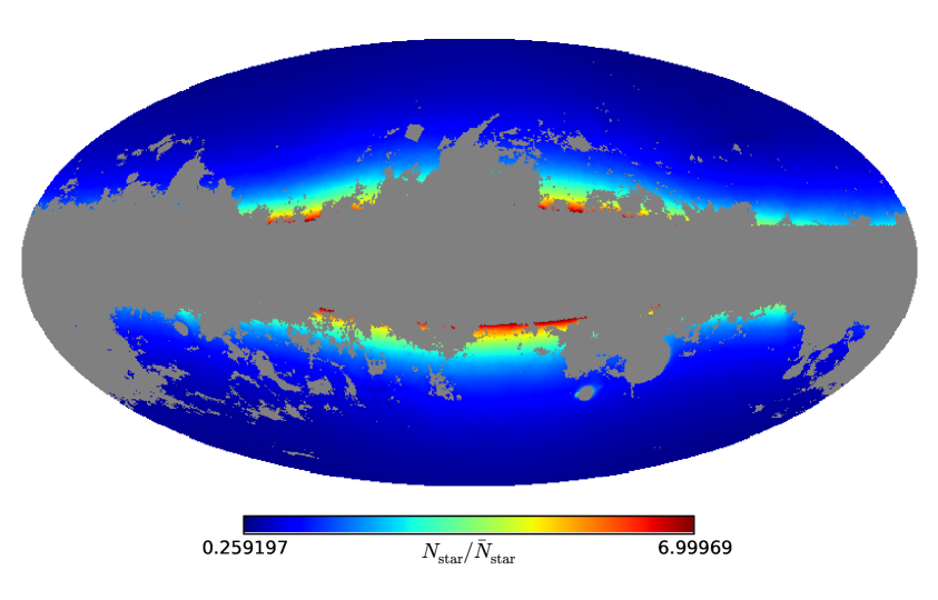
Using the template from Fig. 8, we estimated for all redshift bins with Eq. (3.7). Fig. 9 shows the data variance in template isocontours as a function of the template’s value and our fit. Again, our model describes reasonably well the obscuration effect, apart from the first bin.
We next removed the contamination using a slightly modified version of the approach proposed in [62, 46], i.e. we computed the correlation of the (weighted) data with the contamination template. The weighted number counts are defined as:
| (3.8) |
In the equation above, is our estimate for the obscuration parameter, and the first term inside the square brackets shows we assumed . Deviations from this assumption were studied in [44] and they mostly lead to a small re-scaling of the angular power spectrum; we also verified this effect in our simulations (see Sec. 5). We call the term inside the brackets that multiplies the weighted template.
Now we can compute the average weighted density in the redshift bin over the survey footprint and do the same for the weighted template:
| (3.9) |
where is the unmasked area of the survey. Assuming that the Poisson noise and the true galaxy overdensity do not correlate with our weighted template difference , can be estimated by:
| (3.10) |
where . In practice, we may expect a small random correlation between and , which was investigated and corrected for in [46]. We nevertheless ignore this bias as it does not affect our analysis significantly (see Sec. 5). Lastly, the true mean galaxy density is estimated from the data as:
| (3.11) |
The estimated parameters , and , are presented in Table 1, where we see that both obscuration and contamination are clearly present in all bins. Once more, the first bin shows higher values of systematics, and the estimated error bars are much larger as well, specially for the obscuration parameter. All these difficulties presented by the first bin indicate that its systematics are not as successfully modeled as for the other bins. On top of that, this redshift range is well covered by data with better constrained photo-s, larger sky coverage, and apparently less affected by systematics – namely the 2MPZ catalog [63, 34]. Thus, we decided to ignore the first redshift bin in the subsequent analysis.
| Bin | Photo- range | Mean spec- | |||
|---|---|---|---|---|---|
| 1 | 0.1280 | 0.0902(156) | 0.421(39) | 3.223(48) | |
| 2 | 0.1753 | 0.0681(75) | 0.259(28) | 5.499(41) | |
| 3 | 0.2248 | 0.0735(56) | 0.136(27) | 6.601(33) | |
| 4 | 0.2719 | 0.0818(50) | 0.095(25) | 5.826(23) | |
| 5 | 0.3180 | 0.0674(80) | 0.051(13) | 1.748(08) |
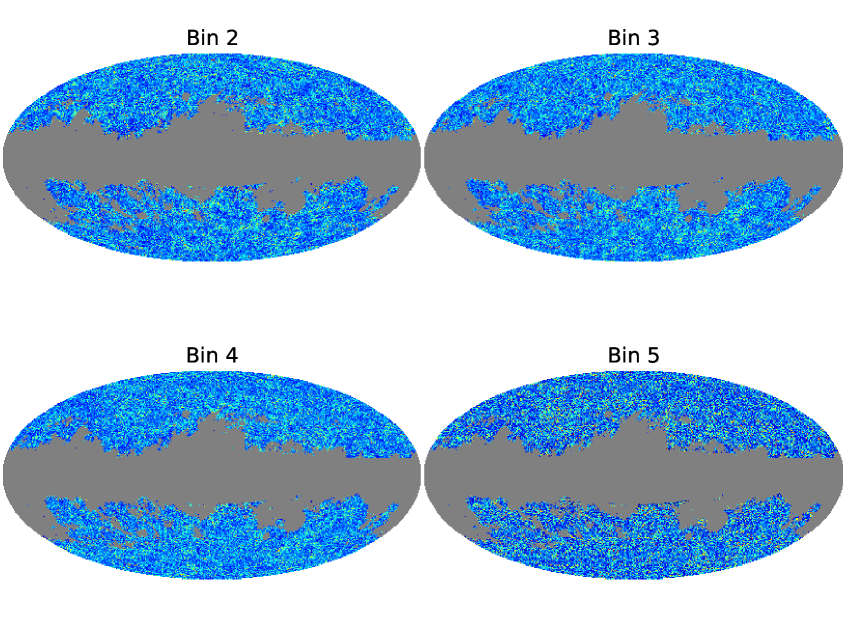
Using the estimated , and , we can solve Eq. (3.2) for inside the survey footprint and estimate the true galaxy density contrast :
| (3.12) |
These are shown in Fig. 10. From Eq. (3.12) we see that, even if our template and our parameter estimates all perfectly match the data, the first term inside the curly brackets might be negative due to Poisson fluctuations in [for instance, might be zero in a given pixel].

4 Methodology for cosmological analysis
4.1 Angular power spectrum estimation
We measured the auto and cross angular power spectra of the WSC density contrast maps using the NaMaster666http://github.com/LSSTDESC/NaMaster code [64], which is based on a pseudo- estimator proposed in [65], and includes further improvements [66, 46]. NaMaster first computes the so-called pseudo power spectra , which measure the variance of the coefficients used to expand the masked density contrast maps in spherical harmonics :
| (4.1) |
The coefficients represent the spherical harmonic transform of the product of the mask and the estimate of the underlying galaxy number density contrast, according to Eq. (3.12). Therefore, when transformed to harmonic space, this product translates into a convolution of the underlying (i.e., full sky) power spectrum and a mixing matrix [66]:

| (4.2) |
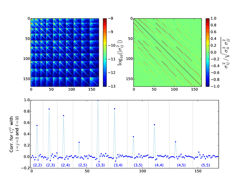
The mixing matrix – determined from the power spectrum of the mask (see e.g. equation 6 of [34]) – is shown in Fig. 11, where we present on the left hand side a 2D color map of the full , while on the left panel we present particular examples of the for three values of . Solving for by inverting the mixing matrix, our final estimate of the true, full-sky angular power spectra is given by:
| (4.3) |
where the denominator removes the effect of the pixelization ( is known as the pixel window function, computed with the Healpix package for our mask resolution) and is the shot-noise contribution, given by:
| (4.4) |
with the Kronecker delta. Table 2 shows that thanks to the large mean number density of galaxies in most redshift bins, the shot-noise term does not dominate on the scales we are interested in. There are two aspects of Eq. (4.4) worth pointing out. First, that these are the full number counts (including contamination by stars) that contribute to the shot-noise. Second, since we weight the data by a factor , the noise is also amplified.
We will present our measurements of the power spectrum in the form of averages in bins of width , and we consider angular scales from .
4.2 Estimation of cosmological parameters
In order to set constraints on cosmological parameters from the measured angular power spectra, we used the Markov Chain Monte Carlo (MCMC) code Montepython777http://baudren.github.io/montepython.html [67, 68]. We have adopted a flat CDM cosmological model with the following free parameters: , where is the Hubble constant; , the baryon density parameter; , the cold dark matter density parameter; , where is the amplitude of the primordial power spectrum; , the spectral index of the primordial power spectrum; the galaxy biases in each of the four redshift bins ; and the widths of the th bin’s spec- selection function as nuisance parameters; in total 13 parameters. We also computed the amplitude of matter density fluctuations as a derived parameter. As priors we used independent Gaussian distributions for parameters poorly constrained by our data: , and , with means and standard deviations according to Planck [69]. We point out that our narrow prior on is translated into prior constraints on as well.
The theoretical s used in the MCMC were computed by CLASS888http://class-code.net [70, 71], including contributions from redshift space distortions and non-linear structure growth [72, 73]. Together with the Planck priors, we applied the extra restriction , to avoid a crash in CLASS caused by reionization happening at too late times. To describe the spec- distribution of galaxies in each photo- bin, we used their Gaussian approximation; the impact of assuming a generalized Lorentzian distribution for the spec-s is discussed in Sec. 7.4.
To reduce the number of possible sources of systematic deviations between measured and true parameters, we restricted our analysis to linear scales. More specifically, for each we only kept the multipoles for which the contribution from the non-linear part of the matter power spectrum was smaller than 10%. Table 2 shows this maximum for each angular power spectrum.
| Bin | Bin | ||
|---|---|---|---|
| 2 | 2 | 70 | 362 |
| 2 | 3 | 80 | – |
| 2 | 4 | 89 | – |
| 2 | 5 | 103 | – |
| 3 | 3 | 93 | 367 |
| 3 | 4 | 104 | – |
| 3 | 5 | 117 | – |
| 4 | 4 | 117 | 316 |
| 4 | 5 | 129 | – |
| 5 | 5 | 140 | 180 |
The binned s were combined into a single data vector with 169 entries. We assumed a Gaussian likelihood, with the covariance (see Fig. 12) extracted from 2500 lognormal mock catalogs of the WSC, described in Sec. 5.1. The s are measured from these mocks, following the same procedure as used for the data (described in Secs. 3.3 and 4.1). The inverse of the covariance matrix estimated from the simulations has been corrected for the finite sample used to estimate it, following [74].
The sampling of the posterior was performed with 10 Markov chains of 100,000 entries, each one starting from a different point in the parameter space. The convergence of the chains was verified using the Gelman-Rubin diagnostic , and all parameters presented .
5 Validation of the analysis
To make sure that all the steps of our analysis work properly, we used the Full-sky Lognormal Astro-fields Simulation Kit (FLASK999http://www.astro.iag.usp.br/~flask) [75] to create hundreds of mock WSC catalogs including the obscuration and contamination effects described in Sec. 3. These mocks are described in detail in Sec. 5.1. The results obtained with our methodology are shown in Sec. 5.2.
5.1 Mock WSC maps
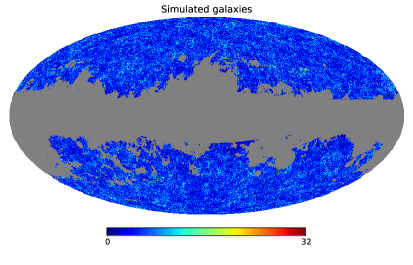
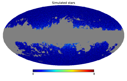
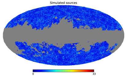
To create lognormal realizations that reproduce the basic statistical properties of the data, FLASK may use as input: a set of auto- and cross-s for all the redshift slices being simulated; the mean density of sources ; and the angular completeness , which includes the mask, obscuration and/or angular variations in density. FLASK output is a set of Healpix maps that include Poisson noise and that reproduce all one- and two-point statistics as required, including cross-correlations between redshift bins. It can also create realizations of stellar densities by assuming , setting to our template and Poisson sampling from it.
As the expected densities (angular-position dependent), we used for galaxies and for stars, where is our template (Fig. 8) and the remaining parameters are set according to Table 1. As input galaxy s we used smooth fits to the measured cleaned s, presented later in Fig. 16, up to . The maps of galaxies and stars, for each bin, were summed into a single map of sources, to which we applied our analysis. Fig. 13 shows an example of such a realization.
5.2 Recovery of mock properties
In this Section we test our methodology to account for the systematic effects and the likelihood machinery on our mock catalogs.
5.2.1 Obscuration and contamination parameters
The first step in our method is to estimate the obscuration and contamination parameters for all bins , along with the mean galaxy density . Table 3 shows the mean and standard deviation of these parameters, recovered from 2500 WSC mock realizations. It shows that our method traces quite well the true values in each of the bins, being able to detect obscuration and contamination at no less than 5.7 and 3.9, respectively. It does, however, produce a detectable average bias of on and on (i.e. overcorrecting, on average, both effects). This bias is likely caused by our simplifying assumption that the cosmological variance for counts-in-pixels, computed from a pixel set, does not depend on the template’s isocontour (Eq. 3.6), which happens to vary both in shape and in area. As density fluctuations are spatially correlated, variances computed in a smaller and compact set will, in general, be smaller. Since, as we show next, this bias does not significantly affect our results, we considered the method’s performance adequate despite of its presence.
| Bin | % bias | % bias | % bias | |||||||||
|---|---|---|---|---|---|---|---|---|---|---|---|---|
| 1 | 0.0902 | 0.0934 | 0.0157 | 3.4 | 0.421 | 0.435 | 0.039 | 3.2 | 3.223 | 3.22 | 0.049 | -0.1 |
| 2 | 0.0681 | 0.0705 | 0.0077 | 3.5 | 0.259 | 0.273 | 0.029 | 5.3 | 5.499 | 5.498 | 0.042 | -0.0 |
| 3 | 0.0735 | 0.0755 | 0.0056 | 2.6 | 0.136 | 0.15 | 0.028 | 9.0 | 6.601 | 6.601 | 0.033 | -0.0 |
| 4 | 0.0818 | 0.0836 | 0.005 | 2.2 | 0.095 | 0.106 | 0.024 | 10.5 | 5.826 | 5.826 | 0.023 | 0.0 |
| 5 | 0.0674 | 0.0703 | 0.0081 | 4.0 | 0.051 | 0.056 | 0.013 | 8.8 | 1.748 | 1.748 | 0.008 | 0.0 |
5.2.2 Angular power spectra
In order to verify the impact of our cleaning method on the s, we processed 750 simulations in three different ways101010Due to the large amount of time required to measure 10 s in three different ways from each simulation, we did not use all 2500 at this step.: (i) we ignored the obscuration and contamination present in them (equivalent to assuming even though they are not); (ii) we only corrected for contamination (equivalent to assuming ); and (iii) we applied the full cleaning method described in Sec. 3.3. We then measured the angular power spectra using our standard procedure (Sec. 4.1). Fig. 14 shows the average of 750 estimated s obtained after applying the three different cleaning processes in comparison to the true in the case of the cross-correlation between redshift bins 3 and 4, as an example. The general characteristics of the results are the same for all bin pairs.
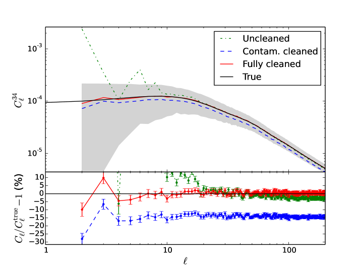
We see that, in our simulations, the typical effect of contamination is to increase the power on the largest scales (), showing at deviations with respect to the true spectrum larger than the error bars. This is clearly a systematic effect we need to correct for in the data. Similarly, we see that correcting only for contamination gives an estimate of the angular power spectrum which is biased low. This bias, also reported in [44], amounts to and reaches the size of the error bars on small scales. After correcting for obscuration, this bias is eliminated (although there seems to be a small positive and constant bias of , possibly caused by an overestimated ). This shows that when measuring cosmological or astrophysical parameters controlling the amplitude of the angular clustering signal (e.g. galaxy bias and primordial spectrum amplitude), correcting for obscuration is a key step to obtain accurate results. This comparison shows that, assuming our modeling of the systematic is correct, its application significantly improves the accuracy of the estimated power spectrum, leaving only possible residual bias which amounts to no more than of the error bars.
5.2.3 Cosmological parameters
Once we have quantified that our cleaning method properly corrects the measured power spectrum, we use the MCMC methodology to recover the input cosmological and nuisance parameters from cleaned s. The input s for the FLASK code were computed by CAMB sources111111http://camb.info/sources [76], including not only contributions from redshift space distortions and non-linearities, but also from a minimal neutrino configuration and all available effects (e.g. gravitational lensing and general relativistic corrections). Furthermore, the computation of the input s did not use the Limber approximation and adopted higher precision than the s sampled by the MCMC. In this way, we verified that any potential deviations in the recovered parameters are not caused by approximation schemes or by the omission of small physical effects. The input s were computed assuming a flat CDM model and Gaussian spec- selection function, and the simulations included the effects of obscuration and contamination. The procedure followed here mimics that applied to the real data.
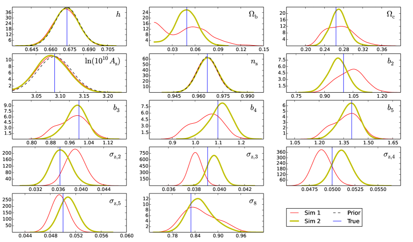
Figure 15 shows that all marginal posterior distributions for all the parameters measured from two independent simulations are compatible with their input values, thus validating our pipeline. We also point out that, while the covariance matrix used in our likelihood was estimated from simulations based on smooth fits to the measured s, the simulated data used in this test was generated from a different set of s, thus attesting that our covariance matrix does not bias the results. The reader might notice that posterior distribution for e.g. from one simulation is displaced from its true value. In this case, we point out that we have 13 independent parameters and, in fact, we should expect a few to deviate from their expected values by chance. The second simulation shows that this is indeed the case. Moreover, we see that the ability to pinpoint is affected by the specific realization of noise and cosmological fluctuations.
6 Results
In Fig. 16 we show the binned angular power spectra measured from the WSC data, both cleaned and uncleaned for contamination and obscuration. We see that the effect of cleaning the WSC is reasonably small on most scales, indicating that galaxy catalogs containing systematics can still provide cosmological information. Despite the smallness of the corrections, we point out two relevant aspects of them: first, applying them significantly reduces the power on the largest scales () in many cases, and as we showed in Sec. 5.2, this is caused by contamination removal; second, some cleaned s show an almost constant-factor increase in power at all scales, caused by obscuration correction, as we have previously discussed (see Fig. 14).
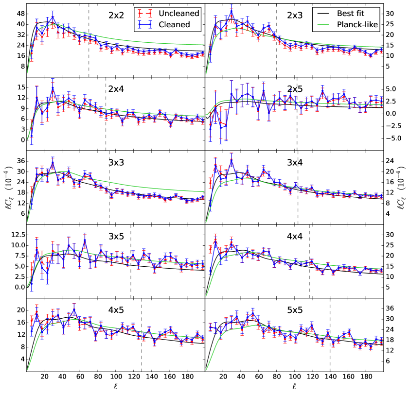
Figure 16 also shows the best-fit model to the cleaned data (black lines), as well as s obtained using cosmological parameters given by Planck [69] and nuisance parameters fitted “by eye” as a rough reference (green lines). By comparing them we see that WSC s present steeper slopes than the fiducial cosmology on the linear scales, and that these slope differences do not seem to be restricted to the largest scales only ().
A comparison of the best-fit obtained under different data processing strategies is presented in Table 4. In every case, the best-fit s and were obtained for that particular dataset by fitting all 13 parameters to it. We see that correcting the WSC count maps for obscuration and contamination improves the fit, but the model remains not very representative of the data. If we ignore multipoles , the fit improves significantly and reaches a -value level that could be considered adequate (larger than ). This may indicate that the largest scales are likely still contaminated even after our corrections, possibly due to a mismatch between the real contamination and our template. If we push the multipole cut to higher values, the agreement does not improve significantly, suggesting that the best-fit is not constrained by the largest scales after this point.
| Approach | d.o.f. | -value | |
|---|---|---|---|
| Uncleaned | 268 | 156 | |
| Cleaned | 237 | 156 | |
| 163 | 136 | ||
| 151 | 126 | ||
| North uncleaned | 398 | 156 | |
| North cleaned | 376 | 156 | |
| North | 148 | 136 | |
| South uncleaned | 248 | 156 | |
| South cleaned | 185 | 156 | |
| South | 157 | 136 |
Figure 17 shows the 1D and 2D posterior distributions for the cosmological parameters that were not directly restricted by Planck priors, for the first three approaches listed in Table 4, and compares them with the values according to Planck. In any case, the posteriors disagree with Planck values by more than . The most discrepant parameter is , which WSC data push to lower values. This is caused by the steep slope of WSC s, as shown in Fig. 16: lower cold matter density leads to less small-scale clustering, tilting the power spectrum and making it redder.
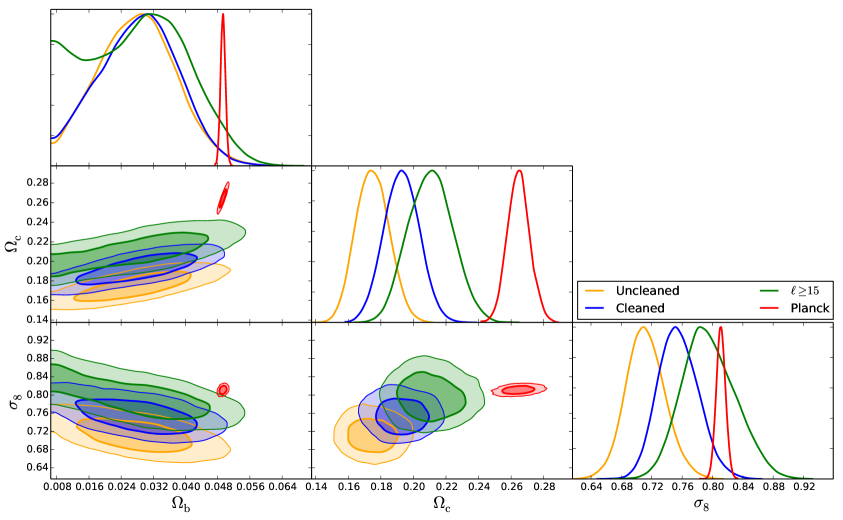
Fig. 17 also shows that the power reduction at the largest scales produced by our cleaning method significantly shifts the posterior closer to the Planck values without increasing its size. This demonstrates, using real data, the importance and advantages of our cleaning method. The removal of the largest scales () moves the posterior even closer to the Planck values but increases its width. This suggests that the stellar density template may be improved, or that the largest scales are affected by extra effects besides stellar obscuration and contamination. In either case, it is clear that identifying and taking these effects into account might be a better approach than ignoring the largest scales altogether, as the latter strategy would lead to worse precision.
7 Robustness tests and search for further systematics
To search for other potential sources of systematic effects in the WSC data, we applied a series of modifications to our analysis and checked their impact on the measured s, using the full-sky cleaned s with as our starting point. One of these tests, already mentioned in Sec. 6, consisted in ignoring scales , with the only impact on the results being that of making the posterior distributions wider.
7.1 Different stellar maps and masks
When considering possible residual systematics related to stellar density, we first raised two hypotheses, viz. (i) that problematic regions near the Galactic bulge could be biasing our results, and (ii) that the Gaussian smoothing applied to the Gaia map could have erased Galactic structures at intermediate scales () that were not removed by our fiducial template. In order to verify these claims, we created the template shown in the left panel of Fig. 18, consisting in an unsmoothed map with regions of stellar density three times the mean masked, and applied it in the removal of obscuration and contamination effects.
Another possibility we considered was that the map obtained from Gaia was not representing the contamination in the WSC. Hence, and based on the cross-match with SDSS presented in Sec. 3.1, we created a template with the simple exponential model given by Eq. (3.1) (central panel in Fig. 18). Finally, a third template was created, in which the model fitted to the matched SDSS stars had an exponential disk (with an extra longitudinal dependence) and a Gaussian bulge (Fig. 18, right panel). Note that despite the fact that this approach is based on a direct estimate of the contamination, it relies on an extrapolation from the SDSS footprint to the whole sky.
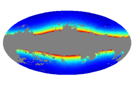
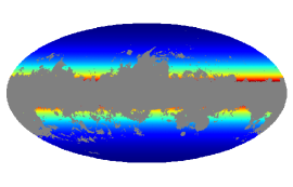
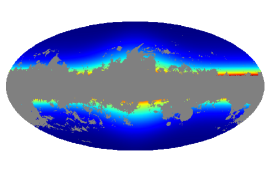
In all cases, the cleaning process reduced the power on the largest scales and only significantly affected multipoles . The two templates based on Gaia led to very similar outcomes and, for most s, improved the results (in terms of large scale power reduction) more than those based on the SDSS cross-match.
7.2 Uncleaned data with
Although we have shown in Secs. 5.2.2 and 5.2.3 that our cleaning method does not bias the results (and, in particular, does not tilt the s), this demonstration assumed that our stellar density template had the correct shape. To test whether our cleaning method could be biasing the results due to a mismatch between the template and the true stellar density distribution, we estimated the posterior distribution of the cosmological parameters from the uncleaned data, while ignoring the largest scales ().
Once more, the posteriors remained highly compatible with those for the cleaned case shown in Fig. 17. This testifies that our cleaning method only affects the large-scale modes and is not responsible for the disagreement between WSC and Planck.
7.3 Mixing matrix deconvolution and prior
As stated in Sec. 4.1, we estimated the angular power spectra of the unmasked sky by inverting Eq. (4.2), that is, we deconvolved the mixing matrix from the data by multiplying the observed pseudo-s by the inverse of the mixing matrix. As this process combines data from different scales, it could transfer to smaller scales the power coming from systematic effects on the largest scales. An alternative analysis that should not suffer from this effect would be to compare the data pseudo-s (after removing shot-noise and the pixel window function) with theoretical s convolved with the mixing matrix . If no anomalous power transfer happens during the mixing matrix deconvolution in the first approach, both methods should yield the same results. We ran the simple test of comparing the ratio between deconvolved data s and fiducial s with the ratio between data pseudo-s and the same (but convolved) fiducial s. Both ratios agreed to very good extent, demonstrating the robustness of our analysis against forward/backward modeling schemes.
Another analysis choice impact we decided to test was that of the prior. It is known that the Hubble constant inferred from Planck () is in tension with direct measurements using type Ia supernovae () [77]. We verified if the Planck prior could be responsible for the observed tension between estimated from WSC and Planck data by replacing it with direct measurements prior. Although this change displaced the WSC posteriors, it actually increased the tension on slightly.
7.4 Redshift distributions
As mentioned in Sec. 2.1, the WSC photo- errors can also be described by a generalized Lorentzian distribution, which results (from Eq. 2.2) in a spec- distribution in each photo- bin that can also be well modeled by the same distribution. To test whether the Gaussianity assumption used in our analysis could bias the results, we employed generalized Lorentzian functions as spec- distributions, and used it to generate a model of s and sample the posterior distribution of the constrained parameters.
Generalized Lorentzian functions have an extra parameter that controls the importance of its tails (see Eq. 2.1). We ran the MCMC under two configurations: (i) we let for each redshift bin vary freely between 1.5 and 4.4; and (ii) we fixed to the values estimated in [38]. In both cases, the posterior on the cosmological parameters remained quite similar to the one in Fig. 17.
We also investigated the scenario in which ignoring the photo- correction due to the north-south hemisphere asymmetry (used in our main analysis; see [33] for details) could bias our results: using the photo- computed directly by ANN, we performed again the redshift binning, the cleaning and the measurement of the . As a result, no significant change was observed.
7.5 Ignoring cross-s
Our main analysis extracted cosmological information not only from the power spectra in each redshift bin but also from the cross-correlation between different bins. These cross-s are more sensitive to the spec- distribution of the galaxies in each bin than the auto-s, since the overlap in the true redshift distributions is one of the main sources of signal in their case. To test if the cross-s could be biasing our results, we repeated the procedure to estimate cosmological parameters using only the auto-s. Although we noticed no significant displacement in the mean values, the width of the 1D posterior distributions are larger, showing that the cross-s do contain extra information.
7.6 Different color and magnitude cuts
The WSC catalog originally had a variable color cut dependent on the distance from the Galactic center, which we removed by applying a more stringent constant cut all over the sky (see Sec. 2.1). We computed the WSC s using this original color cut and verified that it results in more power on the largest scales than when using our cut , without much change on smaller scales. This effect is expected since a position-dependent color cut creates a variable galaxy selection function, likely making their expected number and bias also position-dependent. In other words, the homogeneity in the number counts discussed by [33] is achieved by the original WSC color cut not by removing stars at low latitudes but by removing both stars and galaxies.
Another potential source of systematics is angular variations of the survey depth, caused by changes in observing conditions (in SuperCOSMOS) or total exposure times (number of observations in WISE). To test for the presence of such features, we applied more conservative magnitude cuts, going from the WSC fiducial limits , and to , and . Apart from a constant factor increase in power in all s, expected as a consequence of the larger bias usually associated with brighter galaxies, no significant change was seen in the angular power spectra.
7.7 Analysis by hemispheres
In the full-sky analysis above we have found that, although our corrections for stellar systematics do shift the WSC posterior in the direction of Planck (with respect to the no-correction case), there is still considerable discrepancy between WSC and Planck parameters. As there is no significant evidence from other LSS studies at similar redshifts that this should be physical [78, 34, 79, 35], here we analyze a possible observational effect related to the WSC catalog. Namely, the underlying SuperCOSMOS data are based on measurements from two telescopes which had different effective passbands [53, 80]. The division between the two ‘hemispheres’ is at . As noted in [33], despite color-dependent corrections applied in SuperCOSMOS to match north and south [80], within the WSC flux limits (Sec. 2.1) there is still residual difference in mean galaxy surface density, the north one being up to 4% larger than in the south. As this might be a sign of a genuine systematic in the data, we decided to perform the same analysis as for the full sky also for the two hemispheres. Similar tests were done for 2MPZ [34], which also incorporates SuperCOSMOS as one of the input samples, but no significant differences between resulting cosmological parameters were found. We note that the second input sample included in WSC – WISE – does present non-uniformities in the data but not of hemispherical nature, but rather related to the satellite’s polar orbit and Moon avoidance maneuvers121212See http://wise2.ipac.caltech.edu/docs/release/allsky/expsup/sec3_4.html. Since these non-uniformities are much more involved, we did not investigate their possible impact on our results.
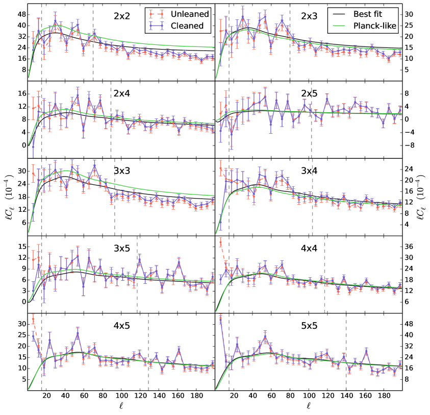
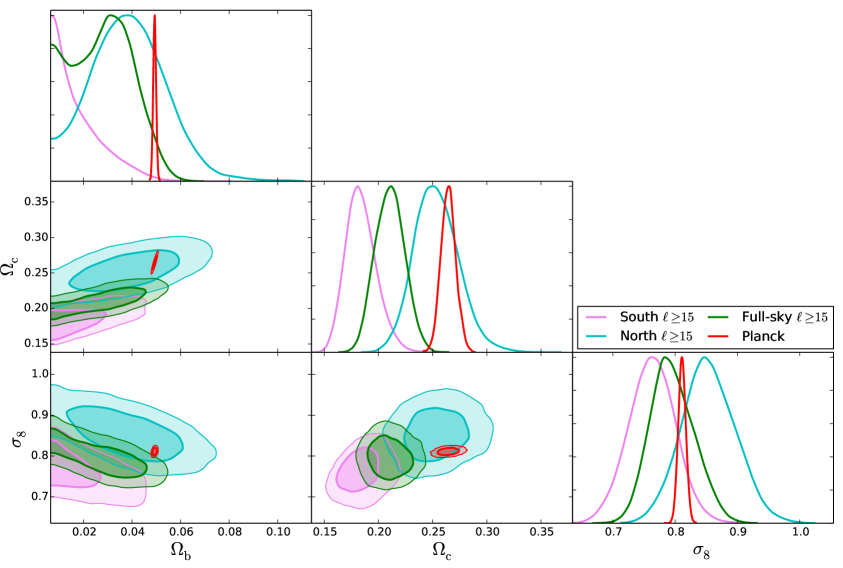
Both hemispheres present similar behavior as the full-sky analysis with respect to the impact of our cleaning process and removal of multipoles . When including all scales with and ignoring contamination, both hemispheres display a bad and a clear tension with the results from Planck. The cleaning process improves the fit and reduces the tension with Planck by lowering the power on the largest scales (). Fig. 19 shows the northern s before and after cleaning. The southern hemisphere – which already presented less excess of power on these scales – is better improved than the northern hemisphere and actually reaches an acceptable , although both remain inconsistent with Planck. When we remove the scales with , the becomes acceptable for both hemispheres, but only the northern hemisphere agrees with Planck. This may indicate that different systematics dominate each hemisphere. The values are shown in Table 4 and the posterior distributions for each hemisphere under the cut are shown and compared with the full-sky posteriors in Fig. 20. The values of all 13 parameters associated with these posteriors are presented in Table 5.
| Full-sky | North | South | ||||
|---|---|---|---|---|---|---|
| Parameter | Best-fit | Mean | Best-fit | Mean | Best-fit | Mean |
8 Conclusions and summary
In this work we have tested a method for estimating and correcting for stellar obscuration and contamination in galaxy redshift catalogs, aiming at extracting cosmological information therefrom. In particular, we have implemented it on the WISESuperCOSMOS (WSC) photo- dataset [33]. We first exposed in Sec. 3 the presence of both systematic effects in WSC, a feature that will be common – albeit with a smaller amplitude – in every photometric survey, including LSST, J-PAS and Euclid. In that Section we also proposed a model for this feature that ties both systematic effects together with a single stellar density template (Eq. 3.2), and showed that such an assumption is supported by the data (Figs. 7 and 9).
The fact that both effects – obscuration and contamination – are linked by the template demands a strategy other than simple correlation [62, 46] to quantify them. We proposed the usage of variance measurements in bands of constant stellar density as a way of determining obscuration (Eq. 3.7), which later can be used to estimate the contamination and real galaxy density (Eqs. 3.10 and 3.11). We verified that this strategy is able to detect and quantify all these parameters with less than 10% bias (Table 3). Although Figs. 14 and 15 show that the effect of any residual bias is negligible in the rest of our analysis, we propose that this cleaning method can be improved if we take into account that galaxy densities are spatially correlated.
It is worth pointing out that one may disentangle the effects of obscuration and contamination directly on the power spectra – since they result in different signatures (see Sec. 5.2.2) – by treating them as nuisance parameters and fitting them together with the cosmology. In this process, it is relevant to not only analyse the data s but also the cross power spectra between data and stellar density template. The contamination level may be better constrained by it, whereas the measurement of obscuration might benefit from a cross- between the template and the observed density difference squared, . Testing this approach should be part of a future work.
All of our methodology was validated by applying it to simulations created by the FLASK code [75] and comparing the measured power spectrum and the constrained parameters with their true input values (see Sec. 5). That analysis demonstrated that applying our cleaning method to data containing obscuration and contamination significantly improved the cosmological parameter inference. This method was also applied to real WSC data, and Table 4 and Fig. 17 show that it improved the power spectra fit at and increased the agreement between the cosmology derived from WSC power spectra and from the Planck satellite.
Despite the improvement obtained both in the full-sky and in separate hemispheres by removing contamination and obscuration, the constraints derived from the angular clustering of WSC still disagree with those derived from the Planck mission if we include the largest scales. In fact, the minimum shows that the standard model is a bad fit to the data in the full-sky and northern hemisphere case (see Table 4) even for parameter values significantly different from Planck. The fit is significantly improved if we ignore multipoles (reaching a -value of 6% for the full-sky case, which could be considered adequate), proving that much of the deviation between data and model happens at the largest scales. The reasons for this excess of power is still unclear and should be further investigated. Possible explanations are that (i) stellar density templates, used to remove contamination, must be improved to better represent WSC true distribution; and that (ii) important systematic effects not related to stars – possibly Galactic extinction and photometric/observational errors – need to be taken into account. We do point out, however, that we have tested three other templates (Fig. reffig:alt-templates) and they have led to similar (or more biased) results.
As the scales are close to the power spectrum turn-over at redshifts probed by WSC, we could claim that the excess of power at scales larger than this comes from physical effects not considered by our cosmological model, e.g.: by non-Gaussian initial conditions caused by certain inflationary models [81]; by the fact that galaxy forms at matter density peaks, which could lead to a scale-dependent bias [30]; or by alternative dark energy models that produce different redshift space distortions [82]. These effects, however, are expected to be small and probably should wait for the investigation of other possible systematics sources. It is worth pointing out that an excess of power is constantly seen on the largest scales of galaxy surveys [47, 34, 35], and due to its correlation with stellar density and other reasons, these modes are mostly discarded. This is unfortunate as the physical effects mentioned above remain untested.
We have tested our data for several potential sources of systematics using the full-sky data limited to as a reference. In Sec. 7 we verified that our results are not affected by photo- error distributions, cleaning strategy, color and magnitude cuts, photo- estimations, mixing matrix deconvolution, the use of cross-s and the restriction to . We did find, however, a hemispherical pattern in the data. Fig. 20 shows that the independent analyses of the two equatorial hemispheres lead to incompatible cosmological parameters: while the analysis restricted to and to the northern hemisphere agrees with Planck (with , and at 95% confidence limit when combined with Planck priors on , and ), the same analysis in the southern hemisphere does not. This difference in extracted cosmological parameters is traced back to different slopes in the measured power spectra, with the southern and full-sky s being steeper than the northern one. Considering it is unlikely that such a large difference has a cosmological origin – especially since cosmological parameters have been extracted from the southern hemisphere before and shown to agree with Planck [34, 79] – this indicates that systematics affecting scales are located in the southern part of WSC data.
Investigating what is the actual source of these systematics is beyond the scope of the present work. One possible explanation is residual miscalibration of SuperCOSMOS data in the south. Namely, the input photographic material for that sample was based on observations from two telescopes (POSS-II in the north and UKST in the south) with effectively different passbands. Despite the efforts to match the passbands using specific color terms, anchored to SDSS as the calibrator [80], differences may still exist. As the WSC sample is selected using maximum apparent magnitude cuts, in particular in the SuperCOSMOS and bands, this may propagate into inconsistent sample selections in the two hemispheres. Indeed, already in [33], a difference in effective source densities between north and south was reported.
However, the most plausible explanation for the north-south difference in large-scale power comes from residual uncertainties in photometric zero points. Where direct SDSS calibration was lacking, plate zero points were given an initial estimate from mean optical-2MASS color, and these values were then perturbed in an attempt to optimize agreement in plate overlap zones. It seems likely that this process will yield zero points that are imperfect at the level of a few hundredths of a magnitude [83], imprinting a pattern of tiles on the galaxy distribution with an rms variation in surface density of several percent. This is the right order of magnitude to cause the offsets that we measure (J. Peacock, private communication). The second input dataset of WSC – WISE – is unlikely to be at the origin of the hemispherical differences as any non-uniformity in that survey is related mostly to telescope’s polar orbit and Moon avoidance strategy. Thus, our present findings seem to suggest that the observed asymmetry is due to residual systematics in the UKST data.
Acknowledgments
The authors thank Vinicius Placco and Laura Sampedro for advice on the use of Gaia data, Filipe Abdalla for comments related to power spectrum measurements and cosmological parameter extraction and John Peacock for valuable information on SuperCOSMOS and useful advice on data analysis and interpretation.
We thank the Wide Field Astronomy Unit (WFAU) at the Institute for Astronomy, Edinburgh, for storing the WISESuperCOSMOS data, available for download from http://ssa.roe.ac.uk/WISExSCOS. We have also made use of data from the European Space Agency (ESA) mission Gaia (https://www.cosmos.esa.int/gaia), processed by the Gaia Data Processing and Analysis Consortium (DPAC, https://www.cosmos.esa.int/web/gaia/dpac/consortium). Funding for the DPAC has been provided by national institutions, in particular the institutions participating in the Gaia Multilateral Agreement. Funding for the Sloan Digital Sky Survey IV has been provided by the Alfred P. Sloan Foundation, the U.S. Department of Energy Office of Science, and the Participating Institutions. SDSS-IV acknowledges support and resources from the Center for High-Performance Computing at the University of Utah. The SDSS web site is http://www.sdss.org. SDSS-IV is managed by the Astrophysical Research Consortium for the Participating Institutions of the SDSS Collaboration including the Brazilian Participation Group, the Carnegie Institution for Science, Carnegie Mellon University, the Chilean Participation Group, the French Participation Group, Harvard-Smithsonian Center for Astrophysics, Instituto de Astrofísica de Canarias, The Johns Hopkins University, Kavli Institute for the Physics and Mathematics of the Universe (IPMU) / University of Tokyo, the Korean Participation Group, Lawrence Berkeley National Laboratory, Leibniz Institut für Astrophysik Potsdam (AIP), Max-Planck-Institut für Astronomie (MPIA Heidelberg), Max-Planck-Institut für Astrophysik (MPA Garching), Max-Planck-Institut für Extraterrestrische Physik (MPE), National Astronomical Observatories of China, New Mexico State University, New York University, University of Notre Dame, Observatário Nacional / MCTI, The Ohio State University, Pennsylvania State University, Shanghai Astronomical Observatory, United Kingdom Participation Group, Universidad Nacional Autónoma de México, University of Arizona, University of Colorado Boulder, University of Oxford, University of Portsmouth, University of Utah, University of Virginia, University of Washington, University of Wisconsin, Vanderbilt University, and Yale University.
This work has made use of the computing facilities of the Laboratory of Astroinformatics (IAG/USP, NAT/Unicsul), whose purchase was made possible by the Brazilian agency FAPESP (grant 2009/54006- 4) and the INCT-A. HSX acknowledges FAPESP Brazilian funding agency for the financial support. ABA acknowledges financial support from the Spanish Ministry of Economy and Competitiveness (MINECO) under the Severo Ochoa program SEV-2015-0548. MB is supported by the Netherlands Organization for Scientific Research, NWO, through grant number 614.001.451 and by the Polish Ministry of Science and Higher Education through grant DIR/WK/2018/12.
References
- [1] A. J. S. Hamilton, M. Tegmark and N. Padmanabhan, Linear redshift distortions and power in the IRAS Point Source Catalog Redshift Survey, MNRAS 317 (2000) L23 [astro-ph/0004334].
- [2] W. J. Percival, C. M. Baugh, J. Bland-Hawthorn, T. Bridges, R. Cannon, S. Cole et al., The 2dF Galaxy Redshift Survey: the power spectrum and the matter content of the Universe, MNRAS 327 (2001) 1297 [astro-ph/0105252].
- [3] M. Tegmark, A. J. S. Hamilton and Y. Xu, The power spectrum of galaxies in the 2dF 100k redshift survey, MNRAS 335 (2002) 887 [astro-ph/0111575].
- [4] S. Cole, W. J. Percival, J. A. Peacock, P. Norberg, C. M. Baugh, C. S. Frenk et al., The 2dF Galaxy Redshift Survey: power-spectrum analysis of the final data set and cosmological implications, MNRAS 362 (2005) 505 [astro-ph/0501174].
- [5] D. J. Eisenstein, I. Zehavi, D. W. Hogg, R. Scoccimarro, M. R. Blanton, R. C. Nichol et al., Detection of the Baryon Acoustic Peak in the Large-Scale Correlation Function of SDSS Luminous Red Galaxies, ApJ 633 (2005) 560 [astro-ph/0501171].
- [6] W. J. Percival, R. C. Nichol, D. J. Eisenstein, J. A. Frieman, M. Fukugita, J. Loveday et al., The Shape of the Sloan Digital Sky Survey Data Release 5 Galaxy Power Spectrum, ApJ 657 (2007) 645 [astro-ph/0608636].
- [7] A. G. Sánchez, E. A. Kazin, F. Beutler, C.-H. Chuang, A. J. Cuesta, D. J. Eisenstein et al., The clustering of galaxies in the SDSS-III Baryon Oscillation Spectroscopic Survey: cosmological constraints from the full shape of the clustering wedges, MNRAS 433 (2013) 1202 [1303.4396].
- [8] M. Yoon, D. Huterer, C. Gibelyou, A. Kovács and I. Szapudi, Dipolar modulation in number counts of WISE-2MASS sources, MNRAS 445 (2014) L60 [1406.1187].
- [9] D. Alonso, A. I. Salvador, F. J. Sánchez, M. Bilicki, J. García-Bellido and E. Sánchez, Homogeneity and isotropy in the Two Micron All Sky Survey Photometric Redshift catalogue, MNRAS 449 (2015) 670 [1412.5151].
- [10] P. Laurent, J.-M. Le Goff, E. Burtin, J.-C. Hamilton, D. W. Hogg, A. Myers et al., A 14 h-3 Gpc3 study of cosmic homogeneity using BOSS DR12 quasar sample, JCAP 11 (2016) 060 [1602.09010].
- [11] C. A. P. Bengaly, Jr., A. Bernui, J. S. Alcaniz, H. S. Xavier and C. P. Novaes, Is there evidence for anomalous dipole anisotropy in the large-scale structure?, MNRAS 464 (2017) 768 [1606.06751].
- [12] F. Avila, C. P. Novaes, A. Bernui and E. de Carvalho, The scale of homogeneity in the local Universe with the ALFALFA catalogue, JCAP 12 (2018) 041 [1806.04541].
- [13] L. Clerkin, D. Kirk, M. Manera, O. Lahav, F. Abdalla, A. Amara et al., Testing the lognormality of the galaxy and weak lensing convergence distributions from Dark Energy Survey maps, MNRAS 466 (2017) 1444 [1605.02036].
- [14] C. Blake, S. Brough, M. Colless, C. Contreras, W. Couch, S. Croom et al., The WiggleZ Dark Energy Survey: the growth rate of cosmic structure since redshift z=0.9, MNRAS 415 (2011) 2876 [1104.2948].
- [15] F. Beutler, S. Saito, H.-J. Seo, J. Brinkmann, K. S. Dawson, D. J. Eisenstein et al., The clustering of galaxies in the SDSS-III Baryon Oscillation Spectroscopic Survey: testing gravity with redshift space distortions using the power spectrum multipoles, MNRAS 443 (2014) 1065 [1312.4611].
- [16] L. Anderson, E. Aubourg, S. Bailey, D. Bizyaev, M. Blanton, A. S. Bolton et al., The clustering of galaxies in the SDSS-III Baryon Oscillation Spectroscopic Survey: baryon acoustic oscillations in the Data Release 9 spectroscopic galaxy sample, MNRAS 427 (2012) 3435 [1203.6594].
- [17] E. de Carvalho, A. Bernui, G. C. Carvalho, C. P. Novaes and H. S. Xavier, Angular Baryon Acoustic Oscillation measure at z=2.225 from the SDSS quasar survey, JCAP 4 (2018) 064 [1709.00113].
- [18] J. A. Peacock, S. Cole, P. Norberg, C. M. Baugh, J. Bland-Hawthorn, T. Bridges et al., A measurement of the cosmological mass density from clustering in the 2dF Galaxy Redshift Survey, Nature 410 (2001) 169 [astro-ph/0103143].
- [19] A. J. Ross, W. J. Percival, A. Carnero, G.-b. Zhao, M. Manera, A. Raccanelli et al., The clustering of galaxies in the SDSS-III DR9 Baryon Oscillation Spectroscopic Survey: constraints on primordial non-Gaussianity, MNRAS 428 (2013) 1116 [1208.1491].
- [20] S. Riemer-Sørensen, C. Blake, D. Parkinson, T. M. Davis, S. Brough, M. Colless et al., WiggleZ Dark Energy Survey: Cosmological neutrino mass constraint from blue high-redshift galaxies, PRD 85 (2012) 081101 [1112.4940].
- [21] A. Loureiro, A. Cuceu, F. B. Abdalla, B. Moraes, L. Whiteway, M. McLeod et al., On The Upper Bound of Neutrino Masses from Combined Cosmological Observations and Particle Physics Experiments, arXiv e-prints (2018) [1811.02578].
- [22] M. Takada, E. Komatsu and T. Futamase, Cosmology with high-redshift galaxy survey: Neutrino mass and inflation, PRD 73 (2006) 083520 [astro-ph/0512374].
- [23] C. Carbone, L. Verde, Y. Wang and A. Cimatti, Neutrino constraints from future nearly all-sky spectroscopic galaxy surveys, JCAP 3 (2011) 030 [1012.2868].
- [24] R. de Putter and O. Doré, Designing an inflation galaxy survey: How to measure (fNL)1 using scale-dependent galaxy bias, PRD 95 (2017) 123513 [1412.3854].
- [25] A. Lewis and A. Challinor, Weak gravitational lensing of the CMB, Phys. Rep. 429 (2006) 1 [astro-ph/0601594].
- [26] Planck Collaboration, P. A. R. Ade, N. Aghanim, C. Armitage-Caplan, M. Arnaud, M. Ashdown et al., Planck 2013 results. XIX. The integrated Sachs-Wolfe effect, A&A 571 (2014) A19 [1303.5079].
- [27] C. Blake and J. Wall, A velocity dipole in the distribution of radio galaxies, Nature 416 (2002) 150 [astro-ph/0203385].
- [28] P. Erdoǧdu, J. P. Huchra, O. Lahav, M. Colless, R. M. Cutri, E. Falco et al., The dipole anisotropy of the 2 Micron All-Sky Redshift Survey, MNRAS 368 (2006) 1515 [astro-ph/0507166].
- [29] M. Bilicki, M. Chodorowski, T. Jarrett and G. A. Mamon, Is the Two Micron All Sky Survey Clustering Dipole Convergent?, ApJ 741 (2011) 31 [1102.4356].
- [30] R. Durrer, A. Gabrielli, M. Joyce and F. Sylos Labini, Bias and the Power Spectrum beyond the Turnover, ApJ 585 (2003) L1 [astro-ph/0211653].
- [31] LSST Science Collaboration, P. A. Abell, J. Allison, S. F. Anderson, J. R. Andrew, J. R. P. Angel et al., LSST Science Book, Version 2.0, arXiv e-prints (2009) arXiv:0912.0201 [0912.0201].
- [32] L. Amendola, S. Appleby, A. Avgoustidis, D. Bacon, T. Baker, M. Baldi et al., Cosmology and fundamental physics with the Euclid satellite, Living Reviews in Relativity 21 (2018) 2 [1606.00180].
- [33] M. Bilicki, J. A. Peacock, T. H. Jarrett, M. E. Cluver, N. Maddox, M. J. I. Brown et al., WISE SuperCOSMOS Photometric Redshift Catalog: 20 Million Galaxies over 3 Steradians, ApJS 225 (2016) 5 [1607.01182].
- [34] A. Balaguera-Antolínez, M. Bilicki, E. Branchini and A. Postiglione, Extracting cosmological information from the angular power spectrum of the 2MASS Photometric Redshift catalogue, MNRAS 476 (2018) 1050 [1711.04583].
- [35] A. Loureiro, B. Moraes, F. B. Abdalla, A. Cuceu, M. McLeod, L. Whiteway et al., ZXCorr: Cosmological Measurements from Angular Power Spectra Analysis of BOSS DR12 Tomography, arXiv e-prints (2018) arXiv:1809.07204 [1809.07204].
- [36] C. A. P. Bengaly, C. P. Novaes, H. S. Xavier, M. Bilicki, A. Bernui and J. S. Alcaniz, The dipole anisotropy of WISE SuperCOSMOS number counts, MNRAS 475 (2018) L106 [1707.08091].
- [37] C. P. Novaes, A. Bernui, H. S. Xavier and G. A. Marques, Tomographic local 2D analyses of the WISExSuperCOSMOS all-sky galaxy catalogue, MNRAS 478 (2018) 3253 [1805.04078].
- [38] J. A. Peacock and M. Bilicki, Wide-area tomography of CMB lensing and the growth of cosmological density fluctuations, MNRAS 481 (2018) 1133 [1805.11525].
- [39] S. Raghunathan, F. Bianchini and C. L. Reichardt, Imprints of gravitational lensing in the Planck cosmic microwave background data at the location of WISESCOS galaxies, PRD 98 (2018) 043506 [1710.09770].
- [40] B. Stölzner, A. Cuoco, J. Lesgourgues and M. Bilicki, Updated tomographic analysis of the integrated Sachs-Wolfe effect and implications for dark energy, PRD 97 (2018) 063506 [1710.03238].
- [41] A. J. Ross, W. J. Percival, A. G. Sánchez, L. Samushia, S. Ho, E. Kazin et al., The clustering of galaxies in the SDSS-III Baryon Oscillation Spectroscopic Survey: analysis of potential systematics, MNRAS 424 (2012) 564 [1203.6499].
- [42] B. Leistedt, H. V. Peiris, D. J. Mortlock, A. Benoit-Lévy and A. Pontzen, Estimating the large-scale angular power spectrum in the presence of systematics: a case study of Sloan Digital Sky Survey quasars, MNRAS 435 (2013) 1857 [1306.0005].
- [43] B. Leistedt and H. V. Peiris, Exploiting the full potential of photometric quasar surveys: optimal power spectra through blind mitigation of systematics, MNRAS 444 (2014) 2 [1404.6530].
- [44] D. L. Shafer and D. Huterer, Multiplicative errors in the galaxy power spectrum: self-calibration of unknown photometric systematics for precision cosmology, MNRAS 447 (2015) 2961 [1410.0035].
- [45] F. Elsner, B. Leistedt and H. V. Peiris, Unbiased methods for removing systematics from galaxy clustering measurements, MNRAS 456 (2016) 2095 [1509.08933].
- [46] F. Elsner, B. Leistedt and H. V. Peiris, Unbiased pseudo-Cℓ power spectrum estimation with mode projection, MNRAS 465 (2017) 1847 [1609.03577].
- [47] S. A. Thomas, F. B. Abdalla and O. Lahav, Excess Clustering on Large Scales in the MegaZ DR7 Photometric Redshift Survey, PRL 106 (2011) 241301 [1012.2272].
- [48] D. G. York, J. Adelman, J. E. Anderson, Jr., S. F. Anderson, J. Annis, N. A. Bahcall et al., The Sloan Digital Sky Survey: Technical Summary, AJ 120 (2000) 1579 [astro-ph/0006396].
- [49] Gaia Collaboration, T. Prusti, J. H. J. de Bruijne, A. G. A. Brown, A. Vallenari, C. Babusiaux et al., The Gaia mission, A&A 595 (2016) A1 [1609.04153].
- [50] Gaia Collaboration, A. G. A. Brown, A. Vallenari, T. Prusti, J. H. J. de Bruijne, C. Babusiaux et al., Gaia Data Release 2. Summary of the contents and survey properties, A&A 616 (2018) A1 [1804.09365].
- [51] R. M. Cutri, E. L. Wright, T. Conrow, J. W. Fowler, P. R. M. Eisenhardt, C. Grillmair et al., Explanatory Supplement to the AllWISE Data Release Products, tech. rep., Nov., 2013.
- [52] E. L. Wright, P. R. M. Eisenhardt, A. K. Mainzer, M. E. Ressler, R. M. Cutri, T. Jarrett et al., The Wide-field Infrared Survey Explorer (WISE): Mission Description and Initial On-orbit Performance, AJ 140 (2010) 1868 [1008.0031].
- [53] N. C. Hambly, H. T. MacGillivray, M. A. Read, S. B. Tritton, E. B. Thomson, B. D. Kelly et al., The SuperCOSMOS Sky Survey - I. Introduction and description, MNRAS 326 (2001) 1279 [astro-ph/0108286].
- [54] N. C. Hambly, M. J. Irwin and H. T. MacGillivray, The SuperCOSMOS Sky Survey - II. Image detection, parametrization, classification and photometry, MNRAS 326 (2001) 1295 [astro-ph/0108290].
- [55] K. M. Górski, E. Hivon, A. J. Banday, B. D. Wandelt, F. K. Hansen, M. Reinecke et al., HEALPix: A Framework for High-Resolution Discretization and Fast Analysis of Data Distributed on the Sphere, ApJ 622 (2005) 759 [astro-ph/0409513].
- [56] A. A. Collister and O. Lahav, ANNz: Estimating Photometric Redshifts Using Artificial Neural Networks, PASP 116 (2004) 345 [astro-ph/0311058].
- [57] S. P. Driver, P. Norberg, I. K. Baldry, S. P. Bamford, A. M. Hopkins, J. Liske et al., GAMA: towards a physical understanding of galaxy formation, Astronomy and Geophysics 50 (2009) 5.12 [0910.5123].
- [58] B. Abolfathi, D. S. Aguado, G. Aguilar, C. Allende Prieto, A. Almeida, T. T. Ananna et al., The Fourteenth Data Release of the Sloan Digital Sky Survey: First Spectroscopic Data from the Extended Baryon Oscillation Spectroscopic Survey and from the Second Phase of the Apache Point Observatory Galactic Evolution Experiment, ApJS 235 (2018) 42 [1707.09322].
- [59] R. H. Lupton, Z. Ivezic, J. E. Gunn, G. Knapp, M. A. Strauss and N. Yasuda, SDSS Imaging Pipelines, in Survey and Other Telescope Technologies and Discoveries (J. A. Tyson and S. Wolff, eds.), vol. 4836 of Proc. SPIE, pp. 350–356, Dec., 2002, DOI.
- [60] J. R. Pier, J. A. Munn, R. B. Hindsley, G. S. Hennessy, S. M. Kent, R. H. Lupton et al., Astrometric Calibration of the Sloan Digital Sky Survey, AJ 125 (2003) 1559 [astro-ph/0211375].
- [61] F. Arenou, X. Luri, C. Babusiaux, C. Fabricius, A. Helmi, T. Muraveva et al., Gaia Data Release 2. Catalogue validation, A&A 616 (2018) A17 [1804.09375].
- [62] G. B. Rybicki and W. H. Press, Interpolation, realization, and reconstruction of noisy, irregularly sampled data, ApJ 398 (1992) 169.
- [63] M. Bilicki, T. H. Jarrett, J. A. Peacock, M. E. Cluver and L. Steward, Two Micron All Sky Survey Photometric Redshift Catalog: A Comprehensive Three-dimensional Census of the Whole Sky, ApJS 210 (2014) 9 [1311.5246].
- [64] D. Alonso, J. Sanchez and A. Slosar, A unified pseudo- framework, arXiv e-prints (2018) [1809.09603].
- [65] P. J. E. Peebles, Statistical Analysis of Catalogs of Extragalactic Objects. I. Theory, ApJ 185 (1973) 413.
- [66] E. Hivon, K. M. Górski, C. B. Netterfield, B. P. Crill, S. Prunet and F. Hansen, MASTER of the Cosmic Microwave Background Anisotropy Power Spectrum: A Fast Method for Statistical Analysis of Large and Complex Cosmic Microwave Background Data Sets, ApJ 567 (2002) 2 [astro-ph/0105302].
- [67] B. Audren, J. Lesgourgues, K. Benabed and S. Prunet, Conservative constraints on early cosmology with MONTE PYTHON, JCAP 2 (2013) 001 [1210.7183].
- [68] T. Brinckmann and J. Lesgourgues, MontePython 3: boosted MCMC sampler and other features, arXiv e-prints (2018) [1804.07261].
- [69] Planck Collaboration, P. A. R. Ade, N. Aghanim, M. Arnaud, M. Ashdown, J. Aumont et al., Planck 2015 results. XIII. Cosmological parameters, A&A 594 (2016) A13 [1502.01589].
- [70] D. Blas, J. Lesgourgues and T. Tram, The Cosmic Linear Anisotropy Solving System (CLASS). Part II: Approximation schemes, JCAP 7 (2011) 034 [1104.2933].
- [71] E. Di Dio, F. Montanari, J. Lesgourgues and R. Durrer, The CLASSgal code for relativistic cosmological large scale structure, JCAP 11 (2013) 044 [1307.1459].
- [72] R. E. Smith, J. A. Peacock, A. Jenkins, S. D. M. White, C. S. Frenk, F. R. Pearce et al., Stable clustering, the halo model and non-linear cosmological power spectra, MNRAS 341 (2003) 1311 [astro-ph/0207664].
- [73] R. Takahashi, M. Sato, T. Nishimichi, A. Taruya and M. Oguri, Revising the Halofit Model for the Nonlinear Matter Power Spectrum, ApJ 761 (2012) 152 [1208.2701].
- [74] J. Hartlap, P. Simon and P. Schneider, Why your model parameter confidences might be too optimistic. Unbiased estimation of the inverse covariance matrix, A&A 464 (2007) 399 [astro-ph/0608064].
- [75] H. S. Xavier, F. B. Abdalla and B. Joachimi, Improving lognormal models for cosmological fields, MNRAS 459 (2016) 3693 [1602.08503].
- [76] A. Challinor and A. Lewis, Linear power spectrum of observed source number counts, PRD 84 (2011) 043516 [1105.5292].
- [77] A. G. Riess, L. M. Macri, S. L. Hoffmann, D. Scolnic, S. Casertano, A. V. Filippenko et al., A 2.4% Determination of the Local Value of the Hubble Constant, ApJ 826 (2016) 56 [1604.01424].
- [78] H. Gil-Marín, L. Verde, J. Noreña, A. J. Cuesta, L. Samushia, W. J. Percival et al., The power spectrum and bispectrum of SDSS DR11 BOSS galaxies - II. Cosmological interpretation, MNRAS 452 (2015) 1914 [1408.0027].
- [79] T. M. C. Abbott, F. B. Abdalla, A. Alarcon, J. Aleksić, S. Allam, S. Allen et al., Dark Energy Survey year 1 results: Cosmological constraints from galaxy clustering and weak lensing, PRD 98 (2018) 043526.
- [80] J. A. Peacock, N. C. Hambly, M. Bilicki, H. T. MacGillivray, L. Miller, M. A. Read et al., The SuperCOSMOS all-sky galaxy catalogue, MNRAS 462 (2016) 2085 [1607.01189].
- [81] N. Dalal, O. Doré, D. Huterer and A. Shirokov, Imprints of primordial non-Gaussianities on large-scale structure: Scale-dependent bias and abundance of virialized objects, PRD 77 (2008) 123514 [0710.4560].
- [82] M. Takada, Can a galaxy redshift survey measure dark energy clustering?, PRD 74 (2006) 043505 [astro-ph/0606533].
- [83] M. F. Skrutskie et al., The Two Micron All Sky Survey (2MASS), AJ 131 (2006) 1163.