Theory and Phenomenology of Two Higgs Doublet Type-II Seesaw
model at the LHC Run-2

B. Ait Ouazghour brahim.aitouazghour@edu.uca.ac.ma LPHEA, Faculty of Science Semlalia, Cadi Ayyad University, P.O.B. 2390 Marrakech, Morocco    A. Arhrib aarhrib@gmail.com Faculty of Sciences and techniques, Abdelmalek Essaadi University, B.P. 416. Tanger, Morocco    R. Benbrik r.benbrik@uca.ac.ma LPHEA, Faculty of Science Semlalia, Cadi Ayyad University, P.O.B. 2390 Marrakech, Morocco MSISM Team, Faculté Polydisciplinaire de Safi, Sidi Bouzid, B.P. 4162, Safi, Morocco    M. Chabab mchabab@uca.ac.ma LPHEA, Faculty of Science Semlalia, Cadi Ayyad University, P.O.B. 2390 Marrakech, Morocco    L. Rahili rahililarbi@gmail.com LPHEA, Faculty of Science Semlalia, Cadi Ayyad University, P.O.B. 2390 Marrakech, Morocco EPTHE, Faculty of Sciences, Ibn Zohr University, B.P 8106, Agadir, Morocco
Abstract

Abstract

We study the most popular scalar extension of the Standard Model, namely the Two Higgs doublet model, extended by a complex triplet scalar (2HDMcT). Such considering model with a very small vacuum expectation value, provides a solution to the massive neutrinos through the so-called type II seesaw mechanism. We show that the 2HDMcT enlarged parameter space allow for a rich and interesting phenomenology compatible with current experimental constraints. In this paper the 2HDMcT is subject to a detailed scrutiny. Indeed, a complete set of tree level unitarity constraints on the coupling parameters of the potential is determined, and the exact tree-level boundedness from below constraints on these couplings are generated for all directions. We then perform an extensive parameter scan in the 2HDMcT parameter space, delimited by the above derived theoretical constraints as well as by experimental limits. We find that an important triplet admixtures are still compatible with the Higgs data and investigate which observables will allow to restrict the triplet nature most effectively in the next runs of the LHC. Finally, we emphasize new production and decay channels and their phenomenological relevance and treatment at the LHC.

I Introduction

After the discovery of a Standard-Model-like Higgs boson at the Large Hadron Collider (LHC) in 2012 Aad:2012tfa ; Chatrchyan:2012ufa , the Standard Model (SM) of particle physics has been established as the most successful theory describing the elementary particles and their interactions. Despite its success, the SM has several drawbacks that have suggested theoretical investigations as well as experimental searches of physics beyond it. As an example, the observed neutrino oscillation cannot be explained within the SM  Patrignani:2016xqp . Indeed, although the SM Higgs field is responsible for the generation of the masses of all known fundamental particles, it is unable to accommodate the tiny observed neutrino masses. Within a renormalisable theory where new heavy fields are introduced, the neutrino masses are generated via the dimension-five Weinberg operator Weinberg:1979sa , this is the so called seesaw mechanism. Different realisations of such a mechanism can be classified into three types: type I Minkowski:1977sc ; GellMann:1980vs ; Yanagida:1979as ; Mohapatra:1979ia ; Schechter:1980gr in which only right-handed neutrinos coupling to the Higgs field, type II Mohapatra:1980yp ; Lazarides:1980nt ; Wetterich:1981bx ; Schechter:1981cv where a new scalar field in the adjoint representation of SU(2)L𝑆𝑈subscript2𝐿SU(2)_{L} and type III Foot:1988aq which involves two extra fermionic fields. In the above seesaw mechanisms heavy fields are supplemented to the SM spectrum in such a way the desired neutrino properties are reproduced once the electroweak symmetry is broken.

In the type II seesaw model, also dubbed Higgs triplet models (HTM), Arhrib:2011uy ; Arhrib:2011vc ; Chabab:2014ara ; Chabab:2015nel ; Arhrib:2014nya ; Camargo:2018uzw , the SM Lagrangian is augmented by a SU(2)L𝑆𝑈subscript2𝐿SU(2)_{L} scalar triplet field ΔΔ\Delta with hypercharge YΔ=2subscript𝑌Δ2Y_{\Delta}=2. In HTM, neutrino masses are proportional to the vacuum expectation value (vev) of the triplet field. Hence, the small values of neutrino masses is guaranteed by the smallness of the triplet vev assumed to be less than 1 GeV and the non-conservation of lepton number which is explicitly broken by a trilinear coupling μ𝜇\mu term in the HTM scalar potential. The latter, protected by symmetry, is naturally small, thus ensuring small neutrino masses. The model spectrum contains several scalar particles, including a pair of singly charged Higgs boson (H±)superscript𝐻plus-or-minus(H^{\pm}) and doubly charged Higgs boson (H±±)superscript𝐻plus-or-minusabsentplus-or-minus(H^{\pm\pm}). In addition, it also predicts a CP-odd neutral scalar (A0)superscript𝐴0(A^{0}) as well as two CP even neutral scalars, hh and H𝐻H. The lightest scalar hh has essentially the same couplings to the fermions and vector bosons as the Higgs boson of the SM within a large region of the HTM parameter space.

By the new discovery of 125 scalar boson at the LHC, the phenomenology of two-Higgs-doublet mod (2HDM) has been investigated broadly in the literature. In the present work, due to the similarity in mass generation mechanism between type-II seesaw and the Higgs mechanism, we extend HTM and focus on the two Higgs double model extension to the type-II seesaw model, displaying phenomenological characteristics notably different from the scalar sector emerging from the HTM. In this context, we study several Higgs processes giving rise to the production times branching ratios of heavy Higgs bosons and focus on. Unlike most of the earlier studies, we consider here a framework where both type I and type II seesaw mechanisms are implemented and contribute to neutrino mass generation. We consider a high integrated luminosity of LHC collisions at a centre-of-mass energy of 13 TeV.

The content of the paper is laid out as follows. In Sec. II, we derive some crucial features of the 2HDMcT, with a focus on the particle content and the scalar potential of the model, followed by discussions on the minimization conditions of the scalar potential and the scalar mass spectra. Besides, in this work we investigate the impact of two new terms introduced in the model scalar potential. Sec. III, is devoted to the study of the theoretical constraints on the scalar potential parameters from tree-level vacuum stability and perturbative unitarity of the scalar sector. In Sec. IV, we further impose the LHC constraints associated with the 125 GeV Higgs boson and its signal strength to delimit the parameter space. Finally, we present some phenomenological aspects in Sec.LABEL:sec:higgs-phynomenology, benchmark points in Sec.VI and summarise our findings in Sec. VII.

II General considerations of 2HDM with triplet

II.1 The Higgs sector

In a model with two Higgs doublets H1,2subscript𝐻12H_{1,2}, the Two Higgs Doublet Type-II Seesaw Model (2HDMcT) contains an additional SU(2)L𝑆𝑈subscript2𝐿SU(2)_{L} triplet Higgs field ΔΔ\Delta with hypercharge Y=2𝑌2Y=2 and lepton number L=2𝐿2L=-2,

H1subscript𝐻1\displaystyle H_{1} =\displaystyle= (ϕ1+ϕ10),H2=(ϕ2+ϕ20),Δ=(δ+/2δ++δ0δ+/2)formulae-sequencesuperscriptsubscriptitalic-ϕ1subscriptsuperscriptitalic-ϕ01subscript𝐻2superscriptsubscriptitalic-ϕ2subscriptsuperscriptitalic-ϕ02Δsuperscript𝛿2superscript𝛿absentsuperscript𝛿0superscript𝛿2\displaystyle\left(\begin{array}[]{c}\phi_{1}^{+}\\ \phi^{0}_{1}\\ \end{array}\right){,}~{}~{}~{}H_{2}=\left(\begin{array}[]{c}\phi_{2}^{+}\\ \phi^{0}_{2}\\ \end{array}\right){,}~{}~{}~{}\Delta=\left(\begin{array}[]{cc}\delta^{+}/\sqrt{2}&\delta^{++}\\ \delta^{0}&-\delta^{+}/\sqrt{2}\\ \end{array}\right) (7)

The most general renormalizable and gauge invariant Lagrangian of the 2HDMcT scalar sector is given by,

\displaystyle\mathcal{L} =\displaystyle= (DμH)(DμH)+Tr(DμΔ)(DμΔ)V(H,Δ)+Yukawasuperscriptsubscript𝐷𝜇𝐻superscript𝐷𝜇𝐻𝑇𝑟superscriptsubscript𝐷𝜇Δsuperscript𝐷𝜇Δ𝑉𝐻ΔsubscriptYukawa\displaystyle(D_{\mu}{H})^{\dagger}(D^{\mu}{H})+Tr(D_{\mu}{\Delta})^{\dagger}(D^{\mu}{\Delta})-V(H,\Delta)+\mathcal{L}_{\rm Yukawa} (8)

where the scalar potential V(H,Δ)𝑉𝐻ΔV(H,\Delta), symmetric under a group SU(2)L×U(1)Y𝑆𝑈subscript2𝐿𝑈subscript1𝑌SU(2)_{L}\times U(1)_{Y}, reads as Chen-Nomura-2014

V(Hi,Δ)=V(H1,H2)+V(Δ)+Vint(H1,H2,Δ)𝑉subscript𝐻𝑖Δ𝑉subscript𝐻1subscript𝐻2𝑉Δsubscript𝑉𝑖𝑛𝑡subscript𝐻1subscript𝐻2Δ\displaystyle V(H_{i},\Delta)=V(H_{1},H_{2})+V(\Delta)+V_{int}(H_{1},H_{2},\Delta) (9)

where :

V(H1,H2)𝑉subscript𝐻1subscript𝐻2\displaystyle V(H_{1},H_{2}) =\displaystyle= m12H1H1+m22H2H2m32(H1H2+H2H1)+λ12(H1H1)2+λ22(H2H2)2subscriptsuperscript𝑚21superscriptsubscript𝐻1subscript𝐻1subscriptsuperscript𝑚22superscriptsubscript𝐻2subscript𝐻2superscriptsubscript𝑚32superscriptsubscript𝐻1subscript𝐻2superscriptsubscript𝐻2subscript𝐻1subscript𝜆12superscriptsuperscriptsubscript𝐻1subscript𝐻12subscript𝜆22superscriptsuperscriptsubscript𝐻2subscript𝐻22\displaystyle m^{2}_{1}\,H_{1}^{\dagger}H_{1}+m^{2}_{2}\,H_{2}^{\dagger}H_{2}-m_{3}^{2}\,\left(H_{1}^{\dagger}H_{2}+H_{2}^{\dagger}H_{1}\right)+\frac{\lambda_{1}}{2}(H_{1}^{\dagger}H_{1})^{2}+\frac{\lambda_{2}}{2}(H_{2}^{\dagger}H_{2})^{2} (10)
+λ3H1H1H2H2+λ4H1H2H2H1+λ52[(H1H2)2+(H2H1)2]subscript𝜆3superscriptsubscript𝐻1subscript𝐻1superscriptsubscript𝐻2subscript𝐻2subscript𝜆4superscriptsubscript𝐻1subscript𝐻2superscriptsubscript𝐻2subscript𝐻1subscript𝜆52delimited-[]superscriptsuperscriptsubscript𝐻1subscript𝐻22superscriptsuperscriptsubscript𝐻2subscript𝐻12\displaystyle+\lambda_{3}\,H_{1}^{\dagger}H_{1}\,H_{2}^{\dagger}H_{2}+\lambda_{4}\,H_{1}^{\dagger}H_{2}\,H_{2}^{\dagger}H_{1}+\frac{\lambda_{5}}{2}\left[(H_{1}^{\dagger}H_{2})^{2}+(H_{2}^{\dagger}H_{1})^{2}\right]
V(Δ)𝑉Δ\displaystyle V(\Delta) =\displaystyle= mΔ2Tr(ΔΔ)+λ¯8(TrΔΔ)2+λ¯9Tr(ΔΔ)2subscriptsuperscript𝑚2Δ𝑇𝑟superscriptΔΔsubscript¯𝜆8superscript𝑇𝑟superscriptΔΔ2subscript¯𝜆9𝑇𝑟superscriptsuperscriptΔΔ2\displaystyle m^{2}_{\Delta}\,Tr(\Delta^{\dagger}{\Delta})+\bar{\lambda}_{8}(Tr\Delta^{\dagger}{\Delta})^{2}+\bar{\lambda}_{9}Tr(\Delta^{\dagger}{\Delta})^{2} (11)
Vint(H1,H2,Δ)subscript𝑉𝑖𝑛𝑡subscript𝐻1subscript𝐻2Δ\displaystyle V_{int}(H_{1},H_{2},\Delta) =\displaystyle= [μ1H1Tiσ2ΔH1+μ2H2Tiσ2ΔH2+μ3H1Tiσ2ΔH2+h.c.]\displaystyle[\mu_{1}H_{1}^{T}{i}\sigma^{2}\Delta^{\dagger}H_{1}+\mu_{2}H_{2}^{T}{i}\sigma^{2}\Delta^{\dagger}H_{2}+\mu_{3}H_{1}^{T}{i}\sigma^{2}\Delta^{\dagger}H_{2}+{\rm h.c.}] (12)
+λ6H1H1TrΔΔ+λ7H2H2TrΔΔ+λ8H1ΔΔH1+λ9H2ΔΔH2subscript𝜆6superscriptsubscript𝐻1subscript𝐻1𝑇𝑟superscriptΔΔsubscript𝜆7superscriptsubscript𝐻2subscript𝐻2𝑇𝑟superscriptΔΔsubscript𝜆8superscriptsubscript𝐻1ΔsuperscriptΔsubscript𝐻1subscript𝜆9superscriptsubscript𝐻2ΔsuperscriptΔsubscript𝐻2\displaystyle+\lambda_{6}\,H_{1}^{\dagger}H_{1}Tr\Delta^{\dagger}{\Delta}+\lambda_{7}\,H_{2}^{\dagger}H_{2}Tr\Delta^{\dagger}{\Delta}+\lambda_{8}\,H_{1}^{\dagger}{\Delta}\Delta^{\dagger}H_{1}+\lambda_{9}\,H_{2}^{\dagger}{\Delta}\Delta^{\dagger}H_{2}

In the above, mi2subscriptsuperscript𝑚2𝑖m^{2}_{i}, i=1,2,3 and mΔ2subscriptsuperscript𝑚2Δm^{2}_{\Delta} are mass squared parameters, λisubscript𝜆𝑖\lambda_{i}, i=1,…,5 are dimensionless couplings not related to the triplet, λ¯isubscript¯𝜆𝑖{\bar{\lambda}_{i}}, i=8,9 are dimensionless couplings related to the triplet field, while μisubscript𝜇𝑖\mu_{i}, i=1,2,3 with λisubscript𝜆𝑖\lambda_{i}, i=6,…,9, are dimensionless couplings that mixe all three Higgs fields. In Eq. 12, Tr𝑇𝑟Tr denotes the trace over 2×2222\times 2 matrices, where for convenience we have used the 2×2222\times 2 traceless matrix representation for the triplet. Also, the potential defined in Eq. 12 exhausts all possible gauge invariant renormalizable operators. For instance, a terms of the form λ10H1ΔΔH1subscript𝜆10superscriptsubscript𝐻1superscriptΔΔsubscript𝐻1\lambda_{10}H_{1}^{\dagger}\Delta^{\dagger}{\Delta}H_{1} and λ11H2ΔΔH2subscript𝜆11superscriptsubscript𝐻2superscriptΔΔsubscript𝐻2\lambda_{11}H_{2}^{\dagger}\Delta^{\dagger}{\Delta}H_{2} Chen-Nomura-2014 , which would be legitimate to add if ΔΔ\Delta contained a singlet component, can actually be projected on the λ6,7subscript𝜆67\lambda_{6,7} and λ8,9subscript𝜆89\lambda_{8,9} operators appearing in Eq. 12 thanks to the identity HiΔΔHi+HiΔΔHisuperscriptsubscript𝐻𝑖superscriptΔΔsubscript𝐻𝑖superscriptsubscript𝐻𝑖ΔsuperscriptΔsubscript𝐻𝑖H_{i}^{\dagger}\Delta^{\dagger}\Delta\,H_{i}+H_{i}^{\dagger}\Delta\Delta^{\dagger}H_{i} =HiHiTr(ΔΔ)absentsuperscriptsubscript𝐻𝑖subscript𝐻𝑖𝑇𝑟superscriptΔΔ=H_{i}^{\dagger}H_{i}Tr(\Delta^{\dagger}{\Delta}) which is valid because ΔΔ\Delta is a traceless 2×2222\times 2 matrix.

Subsequently, we will assume that all these parameters are real valued. Indeed, apart from the μisubscript𝜇𝑖\mu_{i} terms, all the other operators in V(Hi,Δ)𝑉subscript𝐻𝑖ΔV(H_{i},\Delta) are self-conjugate so that, by hermicity of the potential, only the real parts of the λ𝜆\lambda’s and the m12,m22,mΔ2superscriptsubscript𝑚12superscriptsubscript𝑚22superscriptsubscript𝑚Δ2m_{1}^{2},m_{2}^{2},m_{\Delta}^{2} mass parameters are relevant. As for μisubscript𝜇𝑖\mu_{i}, the only parameters that can pick up a would be CP-phases, these phases are unphysical and can always be absorbed in a redefinition of the fields Hisubscript𝐻𝑖H_{i} and ΔΔ\Delta. One thus concludes that the 2HDMcT Lagrangian is CP conserving. The electroweak symmetry is spontaneously broken when the neutral components of the Higgs fields acquire vacuum expectation values v1subscript𝑣1v_{1}, v2subscript𝑣2v_{2} and vtsubscript𝑣𝑡v_{t}. Thus we can shift the Higgs fields in the following way,

ϕ10=v1+ρ1+iη12,ϕ20=v2+ρ2+iη22,δ0=vt+ρ0+iη02formulae-sequencesubscriptsuperscriptitalic-ϕ01subscript𝑣1subscript𝜌1𝑖subscript𝜂12formulae-sequencesubscriptsuperscriptitalic-ϕ02subscript𝑣2subscript𝜌2𝑖subscript𝜂22superscript𝛿0subscript𝑣𝑡subscript𝜌0𝑖subscript𝜂02\displaystyle\phi^{0}_{1}=\frac{v_{1}+\rho_{1}+i\eta_{1}}{\sqrt{2}},\quad\quad\phi^{0}_{2}=\frac{v_{2}+\rho_{2}+i\eta_{2}}{\sqrt{2}},\quad\quad\delta^{0}=\frac{v_{t}+\rho_{0}+i\eta_{0}}{\sqrt{2}} (13)

finding minimization conditions, or tree-level tadpole equations, given by

Vlinear=T1ρ1+T2ρ2+T3ρ0=0,subscript𝑉𝑙𝑖𝑛𝑒𝑎𝑟subscript𝑇1subscript𝜌1subscript𝑇2subscript𝜌2subscript𝑇3subscript𝜌00\displaystyle V_{linear}=T_{1}\rho_{1}+T_{2}\rho_{2}+T_{3}\rho_{0}=0, (14)

where it is safe to take Ti=0subscript𝑇𝑖0T_{i}=0 ( i=1,2,3) which leads to,

m12superscriptsubscript𝑚12\displaystyle m_{1}^{2} =\displaystyle= 2m32v2+2(2μ1v1+μ3v2)vtv1(λ1v12+λ345v22+λ68+vt2)2v12superscriptsubscript𝑚32subscript𝑣222subscript𝜇1subscript𝑣1subscript𝜇3subscript𝑣2subscript𝑣𝑡subscript𝑣1subscript𝜆1superscriptsubscript𝑣12subscript𝜆345superscriptsubscript𝑣22superscriptsubscript𝜆68superscriptsubscript𝑣𝑡22subscript𝑣1\displaystyle\frac{2\,m_{3}^{2}\,v_{2}+\sqrt{2}(2\,\mu_{1}{v_{1}}+\mu_{3}\,v_{2})\,v_{t}-v_{1}\,(\lambda_{1}\,v_{1}^{2}+\lambda_{345}\,v_{2}^{2}+\lambda_{68}^{+}\,v_{t}^{2})}{2\,v_{1}} (15)
m22superscriptsubscript𝑚22\displaystyle m_{2}^{2} =\displaystyle= 2m32v1+2(2μ2v2+μ3v1)vtv2(λ2v22+λ345v12+λ79+vt2)2v22superscriptsubscript𝑚32subscript𝑣122subscript𝜇2subscript𝑣2subscript𝜇3subscript𝑣1subscript𝑣𝑡subscript𝑣2subscript𝜆2superscriptsubscript𝑣22subscript𝜆345superscriptsubscript𝑣12superscriptsubscript𝜆79superscriptsubscript𝑣𝑡22subscript𝑣2\displaystyle\frac{2\,m_{3}^{2}\,v_{1}+\sqrt{2}(2\,\mu_{2}{v_{2}}+\mu_{3}\,v_{1})\,v_{t}-v_{2}\,(\lambda_{2}\,v_{2}^{2}+\lambda_{345}\,v_{1}^{2}+\lambda_{79}^{+}\,v_{t}^{2})}{2\,v_{2}} (16)
mΔ2subscriptsuperscript𝑚2Δ\displaystyle m^{2}_{\Delta} =\displaystyle= 2(μ1v12+v2(μ3v1+μ2v2))vt(λ68+v12+2λ¯89+vt2+λ79+v22)2vt2subscript𝜇1superscriptsubscript𝑣12subscript𝑣2subscript𝜇3subscript𝑣1subscript𝜇2subscript𝑣2subscript𝑣𝑡superscriptsubscript𝜆68superscriptsubscript𝑣122superscriptsubscript¯𝜆89superscriptsubscript𝑣𝑡2superscriptsubscript𝜆79superscriptsubscript𝑣222subscript𝑣𝑡\displaystyle\frac{\sqrt{2}(\mu_{1}{v_{1}^{2}}+v_{2}\,(\mu_{3}{v_{1}}+\mu_{2}{v_{2}}))-v_{t}(\lambda_{68}^{+}v_{1}^{2}+2\bar{\lambda}_{89}^{+}v_{t}^{2}+\lambda_{79}^{+}v_{2}^{2})}{2\,v_{t}} (17)

with λij+=λi+λjsuperscriptsubscript𝜆𝑖𝑗subscript𝜆𝑖subscript𝜆𝑗\lambda_{ij}^{+}=\lambda_{i}+\lambda_{j}, λ¯ij+=λ¯i+λ¯jsuperscriptsubscript¯𝜆𝑖𝑗subscript¯𝜆𝑖subscript¯𝜆𝑗\bar{\lambda}_{ij}^{+}=\bar{\lambda}_{i}+\bar{\lambda}_{j} and λ345=λ3+λ4+λ5subscript𝜆345subscript𝜆3subscript𝜆4subscript𝜆5\lambda_{345}=\lambda_{3}+\lambda_{4}+\lambda_{5}. If the terms associated to vt3superscriptsubscript𝑣𝑡3v_{t}^{3} are omitted in Eq. 17, then we can derive a new expression for vtsubscript𝑣𝑡v_{t} as a function of the triplet scalar mass,

vtμ1v12+μ3v1v2+μ2v222(mΔ2+λ68+v12/2+λ79+v22/2)subscript𝑣𝑡subscript𝜇1superscriptsubscript𝑣12subscript𝜇3subscript𝑣1subscript𝑣2subscript𝜇2superscriptsubscript𝑣222subscriptsuperscript𝑚2Δsuperscriptsubscript𝜆68superscriptsubscript𝑣122superscriptsubscript𝜆79superscriptsubscript𝑣222\displaystyle v_{t}\approx\frac{\mu_{1}v_{1}^{2}+\mu_{3}v_{1}v_{2}+\mu_{2}v_{2}^{2}}{\sqrt{2}(m^{2}_{\Delta}+\lambda_{68}^{+}v_{1}^{2}/2+\lambda_{79}^{+}v_{2}^{2}/2)} (18)

Furthermore, for mΔsubscript𝑚Δm_{\Delta} sufficiently large compared to v1,2subscript𝑣12v_{1,2}, we see that the above formula reduces to, vtμ1v12/2mΔ2similar-tosubscript𝑣𝑡subscript𝜇1subscriptsuperscript𝑣212subscriptsuperscript𝑚2Δv_{t}\sim\mu_{1}v^{2}_{1}/\sqrt{2}m^{2}_{\Delta}, which is referred as type II seesaw mechanism. 111In the absence of μ1subscript𝜇1\mu_{1}, μ2subscript𝜇2\mu_{2} and μ3subscript𝜇3\mu_{3} the mΔ2subscriptsuperscript𝑚2Δm^{2}_{\Delta} becomes negative leading to a spontaneous violation of lepton number. The resulting Higgs spectrum contains a massless triplet scalar, called Majoron J𝐽J. This model was excluded by LEP.

The 2HDMcT model has altogether 242424 degrees of freedom: 21 parameters originating from the scalar potential given by Eq. 9 and tree vacuum expectation values of the Higgs doublets and triplet fields. However, thanks to the three minimisation conditions, the W𝑊W gauge boson mass and the correct electroweak scales, the parameters m12superscriptsubscript𝑚12m_{1}^{2}, m22superscriptsubscript𝑚22m_{2}^{2}, mΔ2superscriptsubscript𝑚Δ2m_{\Delta}^{2} and v𝑣v can be eliminated.

II.2 Higgs masses and mixing angles

In what follows, we will use Eqs. 15, 16 and 17 to trade the mass parameters m112superscriptsubscript𝑚112m_{11}^{2}, m222superscriptsubscript𝑚222m_{22}^{2} and mΔ2superscriptsubscript𝑚Δ2m_{\Delta}^{2} for the rest of parameters given in the potential. Thus, the 14×14141414\times 14 squared mass matrix is given by,

2=122Vηi2|Hi=Hi,Δ=Δsuperscript2evaluated-at12superscript2𝑉superscriptsubscript𝜂𝑖2formulae-sequencesubscript𝐻𝑖delimited-⟨⟩subscript𝐻𝑖Δdelimited-⟨⟩Δ{\mathcal{M}}^{2}=\frac{1}{2}\frac{\partial^{2}V}{\partial\eta_{i}^{2}}|_{H_{i}=\langle H_{i}\rangle,\Delta=\langle\Delta\rangle} (19)

by denoting the corresponding VEV’s

H1=(0v1/2),H2=(0v2/2)andΔ\displaystyle\langle H_{1}\rangle=\left(\begin{array}[]{c}0\\ v_{1}/\sqrt{2}\\ \end{array}\right)~{}~{}~{}~{}{\rm,}~{}~{}~{}~{}\langle H_{2}\rangle=\left(\begin{array}[]{c}0\\ v_{2}/\sqrt{2}\\ \end{array}\right)~{}~{}~{}{\rm and}~{}~{}~{}~{}\langle\Delta\rangle =(00vt/20),absent00subscript𝑣𝑡20\displaystyle=\left(\begin{array}[]{cc}0&0\\ v_{t}/\sqrt{2}&0\\ \end{array}\right)~{}~{}~{},~{}~{}~{}~{}~{} (26)

Eq. 9 can be recast in a block diagonal form of one doubly degenerate eigenvalue mH±±2superscriptsubscript𝑚superscript𝐻plus-or-minusabsentplus-or-minus2m_{H^{\pm\pm}}^{2} and three 3×3333\times 3 matrices denoted in the following by ±2superscriptsubscriptplus-or-minus2{\mathcal{M}}_{\pm}^{2}, 𝒞𝒫odd2superscriptsubscript𝒞subscript𝒫𝑜𝑑𝑑2{\mathcal{M}}_{{\mathcal{CP}}_{odd}}^{2} and 𝒞𝒫even2superscriptsubscript𝒞subscript𝒫𝑒𝑣𝑒𝑛2{\mathcal{M}}_{{\mathcal{CP}}_{even}}^{2}. The bilinear part of the Higgs potential is then given by:

VH1,H2,Δ(2)subscriptsuperscript𝑉2subscript𝐻1subscript𝐻2Δ\displaystyle V^{(2)}_{H_{1},H_{2},\Delta} =\displaystyle= 12(ρ1,ρ2,δ0)𝒞𝒫even2(ρ1ρ2ρ0)+12(η1,η2,η0)𝒞𝒫odd2(η1η2η0)12matrixsubscript𝜌1subscript𝜌2superscript𝛿0superscriptsubscript𝒞subscript𝒫𝑒𝑣𝑒𝑛2matrixsubscript𝜌1subscript𝜌2subscript𝜌012matrixsubscript𝜂1subscript𝜂2subscript𝜂0superscriptsubscript𝒞subscript𝒫𝑜𝑑𝑑2matrixsubscript𝜂1subscript𝜂2subscript𝜂0\displaystyle\frac{1}{2}\begin{pmatrix}\rho_{1},\rho_{2},\delta^{0}\end{pmatrix}\mathcal{M}_{{\mathcal{CP}}_{even}}^{2}\begin{pmatrix}\rho_{1}\\ \rho_{2}\\ \rho_{0}\end{pmatrix}+\frac{1}{2}\begin{pmatrix}\eta_{1},\eta_{2},\eta_{0}\end{pmatrix}\mathcal{M}_{{\mathcal{CP}}_{odd}}^{2}\begin{pmatrix}\eta_{1}\\ \eta_{2}\\ \eta_{0}\end{pmatrix} (27)
+(ϕ1,ϕ2,δ)±2(ϕ1+ϕ2+δ+)+δ++±±2δ,matrixsubscriptsuperscriptitalic-ϕ1subscriptsuperscriptitalic-ϕ2superscript𝛿superscriptsubscriptplus-or-minus2matrixsubscriptsuperscriptitalic-ϕ1subscriptsuperscriptitalic-ϕ2superscript𝛿superscript𝛿absentsuperscriptsubscriptplus-or-minusabsentplus-or-minus2superscript𝛿absent\displaystyle+\begin{pmatrix}\phi^{-}_{1},\phi^{-}_{2},\delta^{-}\end{pmatrix}\mathcal{M}_{\pm}^{2}\begin{pmatrix}\phi^{+}_{1}\\ \phi^{+}_{2}\\ \delta^{+}\end{pmatrix}+\delta^{++}{\mathcal{M}_{\pm\pm}^{2}}\delta^{--}\cdots,

at tree-level. The elements of these mass matrices are explicitly presented below.

Mass of the doubly charged field

The double eigenvalue mH±±2superscriptsubscript𝑚superscript𝐻plus-or-minusabsentplus-or-minus2m_{H^{\pm\pm}}^{2}, corresponding to the doubly charged eigenstate δ±±superscript𝛿plus-or-minusabsentplus-or-minus\delta^{\pm\pm}, can simply be determined by collecting all the coefficients of δ++δsuperscript𝛿absentsuperscript𝛿absent\delta^{++}\delta^{--} in the scalar potential. It is given by reads,

mH±±2=2μ1v12+2μ3v1v2+2μ2v22λ8v12vtλ9v22vt2λ¯9vt32vtsuperscriptsubscript𝑚superscript𝐻plus-or-minusabsentplus-or-minus22subscript𝜇1superscriptsubscript𝑣122subscript𝜇3subscript𝑣1subscript𝑣22subscript𝜇2superscriptsubscript𝑣22subscript𝜆8superscriptsubscript𝑣12subscript𝑣𝑡subscript𝜆9superscriptsubscript𝑣22subscript𝑣𝑡2subscript¯𝜆9superscriptsubscript𝑣𝑡32subscript𝑣𝑡\displaystyle m_{H^{\pm\pm}}^{2}=\frac{\sqrt{2}\mu_{1}v_{1}^{2}+\sqrt{2}\mu_{3}v_{1}v_{2}+\sqrt{2}\mu_{2}v_{2}^{2}-\lambda_{8}v_{1}^{2}v_{t}-\lambda_{9}v_{2}^{2}v_{t}-2\bar{\lambda}_{9}v_{t}^{3}}{2v_{t}} (28)

Mass of the simply charged field

The mass-squared matrix for the simply charged field in the (ϕ1,ϕ2,δsuperscriptsubscriptitalic-ϕ1superscriptsubscriptitalic-ϕ2superscript𝛿\phi_{1}^{-},\phi_{2}^{-},\delta^{-}) basis reads as:

±2=(11±12(λ45+v1v22m32)14(v1A2μ3v2)12(λ45+v1v22m32)22±14(v2B2μ3v1)14(v1A2μ3v2)14(v2B2μ3v1)33±)superscriptsubscriptplus-or-minus2subscriptsuperscriptplus-or-minus1112superscriptsubscript𝜆45subscript𝑣1subscript𝑣22superscriptsubscript𝑚3214subscript𝑣1𝐴2subscript𝜇3subscript𝑣212superscriptsubscript𝜆45subscript𝑣1subscript𝑣22superscriptsubscript𝑚32subscriptsuperscriptplus-or-minus2214subscript𝑣2𝐵2subscript𝜇3subscript𝑣114subscript𝑣1𝐴2subscript𝜇3subscript𝑣214subscript𝑣2𝐵2subscript𝜇3subscript𝑣1subscriptsuperscriptplus-or-minus33\displaystyle{\mathcal{M}}_{\pm}^{2}=\left(\begin{array}[]{ccc}{\mathcal{M}}^{\pm}_{11}&\frac{1}{2}\left(\lambda_{45}^{+}v_{1}v_{2}-2m_{3}^{2}\right)&\frac{1}{4}\left(v_{1}A-2\mu_{3}v_{2}\right)\\ \frac{1}{2}\left(\lambda_{45}^{+}v_{1}v_{2}-2m_{3}^{2}\right)&{\mathcal{M}}^{\pm}_{22}&\frac{1}{4}\left(v_{2}B-2\mu_{3}v_{1}\right)\\ \frac{1}{4}\left(v_{1}A-2\mu_{3}v_{2}\right)&\frac{1}{4}\left(v_{2}B-2\mu_{3}v_{1}\right)&{\mathcal{M}}^{\pm}_{33}\\ \end{array}\right) (32)

where A=2λ8vt4μ1𝐴2subscript𝜆8subscript𝑣𝑡4subscript𝜇1A=\sqrt{2}\lambda_{8}v_{t}-4\mu_{1}, B=2λ9vt4μ2𝐵2subscript𝜆9subscript𝑣𝑡4subscript𝜇2B=\sqrt{2}\lambda_{9}v_{t}-4\mu_{2} and the diagonal terms are given by,

11±subscriptsuperscriptplus-or-minus11\displaystyle{\mathcal{M}}^{\pm}_{11} =\displaystyle= 2m32v2+v1vt(22μ1λ8vt)+2μ3v2vtλ45+v1v222v12superscriptsubscript𝑚32subscript𝑣2subscript𝑣1subscript𝑣𝑡22subscript𝜇1subscript𝜆8subscript𝑣𝑡2subscript𝜇3subscript𝑣2subscript𝑣𝑡superscriptsubscript𝜆45subscript𝑣1superscriptsubscript𝑣222subscript𝑣1\displaystyle\frac{2m_{3}^{2}v_{2}+v_{1}v_{t}\left(2\sqrt{2}\mu_{1}-\lambda_{8}v_{t}\right)+\sqrt{2}\mu_{3}v_{2}v_{t}-\lambda_{45}^{+}v_{1}v_{2}^{2}}{2v_{1}}
22±subscriptsuperscriptplus-or-minus22\displaystyle{\mathcal{M}}^{\pm}_{22} =\displaystyle= 2m32v1+v2vt(22μ2λ9vt)+2μ3v1vtλ45+v12v22v22superscriptsubscript𝑚32subscript𝑣1subscript𝑣2subscript𝑣𝑡22subscript𝜇2subscript𝜆9subscript𝑣𝑡2subscript𝜇3subscript𝑣1subscript𝑣𝑡superscriptsubscript𝜆45superscriptsubscript𝑣12subscript𝑣22subscript𝑣2\displaystyle\frac{2m_{3}^{2}v_{1}+v_{2}v_{t}\left(2\sqrt{2}\mu_{2}-\lambda_{9}v_{t}\right)+\sqrt{2}\mu_{3}v_{1}v_{t}-\lambda_{45}^{+}v_{1}^{2}v_{2}}{2v_{2}}
33±subscriptsuperscriptplus-or-minus33\displaystyle{\mathcal{M}}^{\pm}_{33} =\displaystyle= v12(22μ1λ8vt)+v22(22μ2λ9vt)+22μ3v2v12λ9¯vt34vtsuperscriptsubscript𝑣1222subscript𝜇1subscript𝜆8subscript𝑣𝑡superscriptsubscript𝑣2222subscript𝜇2subscript𝜆9subscript𝑣𝑡22subscript𝜇3subscript𝑣2subscript𝑣12¯subscript𝜆9superscriptsubscript𝑣𝑡34subscript𝑣𝑡\displaystyle\frac{v_{1}^{2}\left(2\sqrt{2}\mu_{1}-\lambda_{8}v_{t}\right)+v_{2}^{2}\left(2\sqrt{2}\mu_{2}-\lambda_{9}v_{t}\right)+2\sqrt{2}\mu_{3}v_{2}v_{1}-2\bar{\lambda_{9}}v_{t}^{3}}{4v_{t}} (33)

Among the three eigenvalues of this matrix, one is zero and corresponds to the charged Goldstone bosons G±superscript𝐺plus-or-minusG^{\pm}, while the two others correspond to the singly charged Higgs bosons denoted by mH1±2superscriptsubscript𝑚superscriptsubscript𝐻1plus-or-minus2m_{H_{1}^{\pm}}^{2} and mH2±2superscriptsubscript𝑚superscriptsubscript𝐻2plus-or-minus2m_{H_{2}^{\pm}}^{2} given by,

mH1,2±2=14v02vt[v0(v0(212±csβseβvt+κ)+22vt2(23±csβ+13±seβ))csβseβ𝒴]subscriptsuperscript𝑚2subscriptsuperscript𝐻plus-or-minus1214superscriptsubscript𝑣02subscript𝑣𝑡delimited-[]minus-or-plussubscript𝑣0subscript𝑣02superscriptsubscript12plus-or-minussubscriptcs𝛽subscriptse𝛽subscript𝑣𝑡𝜅22superscriptsubscript𝑣𝑡2superscriptsubscript23plus-or-minussubscriptcs𝛽superscriptsubscript13plus-or-minussubscriptse𝛽subscriptcs𝛽subscriptse𝛽𝒴\displaystyle m^{2}_{H^{\pm}_{1,2}}=\frac{1}{4v_{0}^{2}v_{t}}\Big{[}-v_{0}\left(v_{0}\left(2{\mathcal{M}}_{12}^{\pm}\text{cs}_{\beta}\text{se}_{\beta}v_{t}+\kappa\right)+2\sqrt{2}v_{t}^{2}\left({\mathcal{M}}_{23}^{\pm}\text{cs}_{\beta}+{\mathcal{M}}_{13}^{\pm}\text{se}_{\beta}\right)\right)\mp\text{cs}_{\beta}\text{se}_{\beta}\sqrt{\mathcal{Y}}\Big{]} (34)

where cxsubscriptc𝑥\text{c}_{x}, sxsubscripts𝑥\text{s}_{x}, csxsubscriptcs𝑥\text{cs}_{x}, sexsubscriptse𝑥\text{se}_{x} stand for the cos(x)𝑥\cos(x), sin(x)𝑥\sin(x), csc(x)𝑥\csc(x), sec(x)𝑥\sec(x) respectively, while v0=v12+v22subscript𝑣0superscriptsubscript𝑣12superscriptsubscript𝑣22v_{0}=\sqrt{v_{1}^{2}+v_{2}^{2}}, v=v12+v22+2vt2𝑣superscriptsubscript𝑣12superscriptsubscript𝑣222superscriptsubscript𝑣𝑡2v=\sqrt{v_{1}^{2}+v_{2}^{2}+2v_{t}^{2}}, κ=2v0(13±cβ+23±sβ)𝜅2subscript𝑣0superscriptsubscript13plus-or-minussubscript𝑐𝛽superscriptsubscript23plus-or-minussubscript𝑠𝛽\kappa=\sqrt{2}v_{0}\left({\mathcal{M}}_{13}^{\pm}c_{\beta}+{\mathcal{M}}_{23}^{\pm}s_{\beta}\right) and

𝒴𝒴\displaystyle\mathcal{Y} =\displaystyle= v02((v0(κcβsβ+212±vt)+22vt2(23±cβ+13±sβ))2\displaystyle v_{0}^{2}\Big{(}\big{(}v_{0}\left(\kappa c_{\beta}s_{\beta}+2{\mathcal{M}}^{\pm}_{12}v_{t}\right)+2\sqrt{2}v_{t}^{2}\left({\mathcal{M}}^{\pm}_{23}c_{\beta}+{\mathcal{M}}^{\pm}_{13}s_{\beta}\right)\big{)}^{2} (35)
\displaystyle- 4v2s2βvt(κ12±+213±23±vt))\displaystyle 4v^{2}s_{2\beta}v_{t}\big{(}\kappa{\mathcal{M}}^{\pm}_{12}+2{\mathcal{M}}^{\pm}_{13}{\mathcal{M}}^{\pm}_{23}v_{t}\big{)}\Big{)}

The above symmetric squared matrix ±2superscriptsubscriptplus-or-minus2{\mathcal{M}}_{\pm}^{2} is diagonalized via 𝒞𝒞{\mathcal{C}} as:

𝒞±2𝒞T𝒞superscriptsubscriptplus-or-minus2superscript𝒞𝑇\displaystyle{\mathcal{C}}{\mathcal{M}}_{\pm}^{2}{\mathcal{C}}^{T} =\displaystyle= diag(mG±2,mH1±2,mH2±2)𝑑𝑖𝑎𝑔subscriptsuperscript𝑚2superscript𝐺plus-or-minussubscriptsuperscript𝑚2superscriptsubscript𝐻1plus-or-minussubscriptsuperscript𝑚2superscriptsubscript𝐻2plus-or-minus\displaystyle diag(m^{2}_{G^{\pm}},m^{2}_{H_{1}^{\pm}},m^{2}_{H_{2}^{\pm}}) (36)

where the 𝒞𝒞{\mathcal{C}} rotation matrix is described by three mixing angles θ1±subscriptsuperscript𝜃plus-or-minus1\theta^{\pm}_{1}, θ2±subscriptsuperscript𝜃plus-or-minus2\theta^{\pm}_{2} and θ3±subscriptsuperscript𝜃plus-or-minus3\theta^{\pm}_{3}, and the corresponding expressions for the 𝒞𝒞{\mathcal{C}} elements are give in Appendix A as a function of the parameters inputs of our model.

Mass of the neutral pseudo-scalar field

As to the mass-squared matrix for the neutral 𝒞𝒫odd𝒞subscript𝒫𝑜𝑑𝑑{{\mathcal{CP}}_{odd}} pseudoscalar field in the basis (η1,η2,η0subscript𝜂1subscript𝜂2subscript𝜂0\eta_{1},\eta_{2},\eta_{0}), it is expressed as:

odd2=(11odd2m32+2μ3vt+2λ5v1v222μ1v1+μ3v222m32+2μ3vt+2λ5v1v2222odd2μ2v2+μ3v122μ1v1+μ3v222μ2v2+μ3v1233odd)superscriptsubscript𝑜𝑑𝑑2superscriptsubscript11𝑜𝑑𝑑2superscriptsubscript𝑚322subscript𝜇3subscript𝑣𝑡2subscript𝜆5subscript𝑣1subscript𝑣222subscript𝜇1subscript𝑣1subscript𝜇3subscript𝑣222superscriptsubscript𝑚322subscript𝜇3subscript𝑣𝑡2subscript𝜆5subscript𝑣1subscript𝑣22superscriptsubscript22𝑜𝑑𝑑2subscript𝜇2subscript𝑣2subscript𝜇3subscript𝑣122subscript𝜇1subscript𝑣1subscript𝜇3subscript𝑣222subscript𝜇2subscript𝑣2subscript𝜇3subscript𝑣12superscriptsubscript33𝑜𝑑𝑑\displaystyle{\mathcal{M}}_{odd}^{2}=\left(\begin{array}[]{ccc}{\mathcal{M}}_{11}^{odd}&\frac{-2m_{3}^{2}+\sqrt{2}\mu_{3}v_{t}+2\lambda_{5}v_{1}v_{2}}{2}&-\frac{2\mu_{1}v_{1}+\mu_{3}v_{2}}{\sqrt{2}}\\ \frac{-2m_{3}^{2}+\sqrt{2}\mu_{3}v_{t}+2\lambda_{5}v_{1}v_{2}}{2}&{\mathcal{M}}_{22}^{odd}&-\frac{2\mu_{2}v_{2}+\mu_{3}v_{1}}{\sqrt{2}}\\ -\frac{2\mu_{1}v_{1}+\mu_{3}v_{2}}{\sqrt{2}}&-\frac{2\mu_{2}v_{2}+\mu_{3}v_{1}}{\sqrt{2}}&{\mathcal{M}}_{33}^{odd}\end{array}\right) (40)

the diagonal terms are given by,

11oddsuperscriptsubscript11𝑜𝑑𝑑\displaystyle{\mathcal{M}}_{11}^{odd} =\displaystyle= 2m32v2+42μ1v1vt+2μ3v2vt2λ5v1v222v12superscriptsubscript𝑚32subscript𝑣242subscript𝜇1subscript𝑣1subscript𝑣𝑡2subscript𝜇3subscript𝑣2subscript𝑣𝑡2subscript𝜆5subscript𝑣1superscriptsubscript𝑣222subscript𝑣1\displaystyle\frac{2m_{3}^{2}v_{2}+4\sqrt{2}\mu_{1}v_{1}v_{t}+\sqrt{2}\mu_{3}v_{2}v_{t}-2\lambda_{5}v_{1}v_{2}^{2}}{2v_{1}}
22oddsuperscriptsubscript22𝑜𝑑𝑑\displaystyle{\mathcal{M}}_{22}^{odd} =\displaystyle= 2m32v1+42μ2v2vt+2μ3v1vt2λ5v12v22v22superscriptsubscript𝑚32subscript𝑣142subscript𝜇2subscript𝑣2subscript𝑣𝑡2subscript𝜇3subscript𝑣1subscript𝑣𝑡2subscript𝜆5superscriptsubscript𝑣12subscript𝑣22subscript𝑣2\displaystyle\frac{2m_{3}^{2}v_{1}+4\sqrt{2}\mu_{2}v_{2}v_{t}+\sqrt{2}\mu_{3}v_{1}v_{t}-2\lambda_{5}v_{1}^{2}v_{2}}{2v_{2}}
33oddsuperscriptsubscript33𝑜𝑑𝑑\displaystyle{\mathcal{M}}_{33}^{odd} =\displaystyle= η1v12+μ3v2v1+μ2v222vtsubscript𝜂1superscriptsubscript𝑣12subscript𝜇3subscript𝑣2subscript𝑣1subscript𝜇2superscriptsubscript𝑣222subscript𝑣𝑡\displaystyle\frac{\eta_{1}v_{1}^{2}+\mu_{3}v_{2}v_{1}+\mu_{2}v_{2}^{2}}{\sqrt{2}v_{t}} (41)

here, 𝒞𝒫odd2superscriptsubscript𝒞subscript𝒫𝑜𝑑𝑑2{\mathcal{M}}_{{\mathcal{CP}}_{odd}}^{2} has three eigenvalues, one is zero corresponding to the neutral Goldstone boson G0superscript𝐺0G^{0} while the two others are the physical states 𝒞𝒫odd𝒞subscript𝒫𝑜𝑑𝑑{{\mathcal{CP}}_{odd}} A1subscript𝐴1A_{1} and A2subscript𝐴2A_{2}, by setting,

ϱitalic-ϱ\displaystyle\varrho =\displaystyle= 23oddcβ+13oddsβsuperscriptsubscript23𝑜𝑑𝑑subscript𝑐𝛽superscriptsubscript13𝑜𝑑𝑑subscript𝑠𝛽\displaystyle{\mathcal{M}}_{23}^{odd}c_{\beta}+{\mathcal{M}}_{13}^{odd}s_{\beta}
ϝitalic-ϝ\displaystyle\digamma =\displaystyle= 13oddcβ+23oddsβsuperscriptsubscript13𝑜𝑑𝑑subscript𝑐𝛽superscriptsubscript23𝑜𝑑𝑑subscript𝑠𝛽\displaystyle{\mathcal{M}}_{13}^{odd}c_{\beta}+{\mathcal{M}}_{23}^{odd}s_{\beta} (42)
𝒳𝒳\displaystyle\mathcal{X} =\displaystyle= [v02((v02ϝcβsβ+212oddv0vt+4ϱvt2)24s2βvt(4vt2+v02)(213odd23odvt+12oddv0ϝ))]\displaystyle\Big{[}v_{0}^{2}\left(\left(v_{0}^{2}\digamma c_{\beta}s_{\beta}+2{\mathcal{M}}_{12}^{odd}v_{0}v_{t}+4\varrho v_{t}^{2}\right){}^{2}-4s_{2\beta}v_{t}\left(4v_{t}^{2}+v_{0}^{2}\right)\left(2{\mathcal{M}}_{13}^{odd}{\mathcal{M}}_{23}^{od}v_{t}+{\mathcal{M}}_{12}^{odd}v_{0}\digamma\right)\right)\Big{]}

theirs masses read as,

mA1,22=14v02vt[v0(2csβseβvt(12oddv0+2ϱvt)+v02ϝ)csβseβ𝒳]subscriptsuperscript𝑚2subscript𝐴1214superscriptsubscript𝑣02subscript𝑣𝑡delimited-[]minus-or-plussubscript𝑣02subscriptcs𝛽subscriptse𝛽subscript𝑣𝑡superscriptsubscript12𝑜𝑑𝑑subscript𝑣02italic-ϱsubscript𝑣𝑡superscriptsubscript𝑣02italic-ϝsubscriptcs𝛽subscriptse𝛽𝒳\displaystyle m^{2}_{A_{1,2}}=\frac{1}{4v_{0}^{2}v_{t}}\Big{[}-v_{0}\left(2\text{cs}_{\beta}\text{se}_{\beta}v_{t}\left({\mathcal{M}}_{12}^{odd}v_{0}+2\varrho v_{t}\right)+v_{0}^{2}\digamma\right)\mp\text{cs}_{\beta}\text{se}_{\beta}\sqrt{\mathcal{X}}\Big{]} (43)

while the diagonalization of such matrix is done in this case by the introduction of an unitary matrix 𝒪𝒪{\mathcal{O}} described by three mixing angles β1subscript𝛽1\beta_{1}, β2subscript𝛽2\beta_{2} and β3subscript𝛽3\beta_{3} whose expressions can be found in the appendix A as,

𝒪𝒞𝒫odd2𝒪T𝒪superscriptsubscript𝒞subscript𝒫𝑜𝑑𝑑2superscript𝒪𝑇\displaystyle{\mathcal{O}}{\mathcal{M}}_{{{\mathcal{CP}}_{odd}}}^{2}{\mathcal{O}}^{T} =\displaystyle= diag(mG02,mA12,mA22)𝑑𝑖𝑎𝑔subscriptsuperscript𝑚2superscript𝐺0subscriptsuperscript𝑚2subscript𝐴1subscriptsuperscript𝑚2subscript𝐴2\displaystyle diag(m^{2}_{G^{0}},m^{2}_{A_{1}},m^{2}_{A_{2}}) (44)

Mass of the neutral scalar field

In the basis (ρ1,ρ2,ρ0subscript𝜌1subscript𝜌2subscript𝜌0\rho_{1},\rho_{2},\rho_{0}) the neutral scalar mass matrix reads :

𝒞𝒫even2=(mρ1ρ12mρ2ρ12mρ0ρ12mρ1ρ22mρ2ρ22mρ0ρ22mρ1ρ02mρ2ρ02mρ0ρ02)superscriptsubscript𝒞subscript𝒫𝑒𝑣𝑒𝑛2superscriptsubscript𝑚subscript𝜌1subscript𝜌12superscriptsubscript𝑚subscript𝜌2subscript𝜌12superscriptsubscript𝑚subscript𝜌0subscript𝜌12superscriptsubscript𝑚subscript𝜌1subscript𝜌22superscriptsubscript𝑚subscript𝜌2subscript𝜌22superscriptsubscript𝑚subscript𝜌0subscript𝜌22superscriptsubscript𝑚subscript𝜌1subscript𝜌02superscriptsubscript𝑚subscript𝜌2subscript𝜌02superscriptsubscript𝑚subscript𝜌0subscript𝜌02\displaystyle{\mathcal{M}}_{{\mathcal{CP}}_{even}}^{2}=\left(\begin{array}[]{ccc}m_{\rho_{1}\rho_{1}}^{2}&m_{\rho_{2}\rho_{1}}^{2}&m_{\rho_{0}\rho_{1}}^{2}\\ m_{\rho_{1}\rho_{2}}^{2}&m_{\rho_{2}\rho_{2}}^{2}&m_{\rho_{0}\rho_{2}}^{2}\\ m_{\rho_{1}\rho_{0}}^{2}&m_{\rho_{2}\rho_{0}}^{2}&m_{\rho_{0}\rho_{0}}^{2}\end{array}\right) (48)

Its diagonal terms are,

mρ1ρ12superscriptsubscript𝑚subscript𝜌1subscript𝜌12\displaystyle m_{\rho_{1}\rho_{1}}^{2} =\displaystyle= λ1v12+v2(2m32+μ3vt)2v1subscript𝜆1superscriptsubscript𝑣12subscript𝑣22superscriptsubscript𝑚32subscript𝜇3subscript𝑣𝑡2subscript𝑣1\displaystyle\lambda_{1}v_{1}^{2}+\frac{v_{2}\left(\sqrt{2}m_{3}^{2}+\mu_{3}v_{t}\right)}{\sqrt{2}v_{1}}
mρ2ρ22superscriptsubscript𝑚subscript𝜌2subscript𝜌22\displaystyle m_{\rho_{2}\rho_{2}}^{2} =\displaystyle= λ2v22+v1(2m32+μ3vt)2v2subscript𝜆2superscriptsubscript𝑣22subscript𝑣12superscriptsubscript𝑚32subscript𝜇3subscript𝑣𝑡2subscript𝑣2\displaystyle\lambda_{2}v_{2}^{2}+\frac{v_{1}\left(\sqrt{2}m_{3}^{2}+\mu_{3}v_{t}\right)}{\sqrt{2}v_{2}}
mρ0ρ02superscriptsubscript𝑚subscript𝜌0subscript𝜌02\displaystyle m_{\rho_{0}\rho_{0}}^{2} =\displaystyle= 4(λ¯8+λ¯9)vt3+2(μ1v12+μ3v2v1+μ2v22)2vt4subscript¯𝜆8subscript¯𝜆9superscriptsubscript𝑣𝑡32subscript𝜇1superscriptsubscript𝑣12subscript𝜇3subscript𝑣2subscript𝑣1subscript𝜇2superscriptsubscript𝑣222subscript𝑣𝑡\displaystyle\frac{4\left(\bar{\lambda}_{8}+\bar{\lambda}_{9}\right)v_{t}^{3}+\sqrt{2}\left(\mu_{1}v_{1}^{2}+\mu_{3}v_{2}v_{1}+\mu_{2}v_{2}^{2}\right)}{2v_{t}} (49)

while the off-diagonal terms are given by,

mρ2ρ12superscriptsubscript𝑚subscript𝜌2subscript𝜌12\displaystyle m_{\rho_{2}\rho_{1}}^{2} =\displaystyle= mρ1ρ22=12(2v1v2λ3452m32μ3vt)superscriptsubscript𝑚subscript𝜌1subscript𝜌22122subscript𝑣1subscript𝑣2subscript𝜆3452superscriptsubscript𝑚32subscript𝜇3subscript𝑣𝑡\displaystyle m_{\rho_{1}\rho_{2}}^{2}=\frac{1}{\sqrt{2}}\left(\sqrt{2}v_{1}v_{2}\lambda_{345}-\sqrt{2}m_{3}^{2}-\mu_{3}v_{t}\right)
mρ0ρ12superscriptsubscript𝑚subscript𝜌0subscript𝜌12\displaystyle m_{\rho_{0}\rho_{1}}^{2} =\displaystyle= mρ1ρ02=12(2v1vt(λ6+λ8)(2μ1v1+μ3v2))superscriptsubscript𝑚subscript𝜌1subscript𝜌02122subscript𝑣1subscript𝑣𝑡subscript𝜆6subscript𝜆82subscript𝜇1subscript𝑣1subscript𝜇3subscript𝑣2\displaystyle m_{\rho_{1}\rho_{0}}^{2}=\frac{1}{\sqrt{2}}\left(\sqrt{2}v_{1}v_{t}(\lambda_{6}+\lambda_{8})-(2\mu_{1}v_{1}+\mu_{3}v_{2})\right)
mρ0ρ22superscriptsubscript𝑚subscript𝜌0subscript𝜌22\displaystyle m_{\rho_{0}\rho_{2}}^{2} =\displaystyle= mρ2ρ02=12(2v2vt(λ7+λ9)(2μ2v2+μ3v1))superscriptsubscript𝑚subscript𝜌2subscript𝜌02122subscript𝑣2subscript𝑣𝑡subscript𝜆7subscript𝜆92subscript𝜇2subscript𝑣2subscript𝜇3subscript𝑣1\displaystyle m_{\rho_{2}\rho_{0}}^{2}=\frac{1}{\sqrt{2}}\left(\sqrt{2}v_{2}v_{t}(\lambda_{7}+\lambda_{9})-(2\mu_{2}v_{2}+\mu_{3}v_{1})\right) (50)

The mass matrix can be diagonalised by an orthogonal matrix {\mathcal{E}} which we parametrise as

=(cα1cα2sα1cα2sα2(cα1sα2sα3+sα1cα3)cα1cα3sα1sα2sα3cα2sα3cα1sα2cα3+sα1sα3(cα1sα3+sα1sα2cα3)cα2cα3)subscript𝑐subscript𝛼1subscript𝑐subscript𝛼2subscript𝑠subscript𝛼1subscript𝑐subscript𝛼2subscript𝑠subscript𝛼2subscript𝑐subscript𝛼1subscript𝑠subscript𝛼2subscript𝑠subscript𝛼3subscript𝑠subscript𝛼1subscript𝑐subscript𝛼3subscript𝑐subscript𝛼1subscript𝑐subscript𝛼3subscript𝑠subscript𝛼1subscript𝑠subscript𝛼2subscript𝑠subscript𝛼3subscript𝑐subscript𝛼2subscript𝑠subscript𝛼3subscript𝑐subscript𝛼1subscript𝑠subscript𝛼2subscript𝑐subscript𝛼3subscript𝑠subscript𝛼1subscript𝑠subscript𝛼3subscript𝑐subscript𝛼1subscript𝑠subscript𝛼3subscript𝑠subscript𝛼1subscript𝑠subscript𝛼2subscript𝑐subscript𝛼3subscript𝑐subscript𝛼2subscript𝑐subscript𝛼3\displaystyle{\mathcal{E}}=\left(\begin{array}[]{ccc}c_{\alpha_{1}}c_{\alpha_{2}}&s_{\alpha_{1}}c_{\alpha_{2}}&s_{\alpha_{2}}\\ -(c_{\alpha_{1}}s_{\alpha_{2}}s_{\alpha_{3}}+s_{\alpha_{1}}c_{\alpha_{3}})&c_{\alpha_{1}}c_{\alpha_{3}}-s_{\alpha_{1}}s_{\alpha_{2}}s_{\alpha_{3}}&c_{\alpha_{2}}s_{\alpha_{3}}\\ -c_{\alpha_{1}}s_{\alpha_{2}}c_{\alpha_{3}}+s_{\alpha_{1}}s_{\alpha_{3}}&-(c_{\alpha_{1}}s_{\alpha_{3}}+s_{\alpha_{1}}s_{\alpha_{2}}c_{\alpha_{3}})&c_{\alpha_{2}}c_{\alpha_{3}}\end{array}\right) (54)

where the mixing angles α1subscript𝛼1\alpha_{1}, α2subscript𝛼2\alpha_{2} and α3subscript𝛼3\alpha_{3} can be chosen in the range

π2α1,2,3π2.𝜋2subscript𝛼123𝜋2\displaystyle-\frac{\pi}{2}\leq\alpha_{1,2,3}\leq\frac{\pi}{2}\;. (55)

the rotation between the two basis (ρ1,ρ2,ρ0subscript𝜌1subscript𝜌2subscript𝜌0\rho_{1},\rho_{2},\rho_{0}) and (h1,h2,h3subscript1subscript2subscript3h_{1},h_{2},h_{3}) diagonalises the mass matrix 𝒞𝒫even2superscriptsubscript𝒞subscript𝒫𝑒𝑣𝑒𝑛2{\mathcal{M}}_{{\mathcal{CP}}_{even}}^{2} as,

𝒞𝒫even2Tsuperscriptsubscript𝒞subscript𝒫𝑒𝑣𝑒𝑛2superscript𝑇\displaystyle{\mathcal{E}}{\mathcal{M}}_{{{\mathcal{CP}}_{even}}}^{2}{\mathcal{E}}^{T} =\displaystyle= diag(mh12,mh22,mh32)𝑑𝑖𝑎𝑔subscriptsuperscript𝑚2subscript1subscriptsuperscript𝑚2subscript2subscriptsuperscript𝑚2subscript3\displaystyle diag(m^{2}_{h_{1}},m^{2}_{h_{2}},m^{2}_{h_{3}}) (56)

and leads to three mass eigenstates, ordered by ascending mass as:

mh12<mh22<mh32.subscriptsuperscript𝑚2subscript1subscriptsuperscript𝑚2subscript2subscriptsuperscript𝑚2subscript3\displaystyle m^{2}_{h_{1}}<m^{2}_{h_{2}}<m^{2}_{h_{3}}\;. (57)

One choice of input parameters implemented in 2HDMcT consistes to use the following hybrid parameterisation,

𝒫I={α1,α2,α3,mh1,mh2,mh3,mH±±,λ1,λ3,λ4,λ6,λ8,λ¯8,λ¯9,μ1,vt,tanβ}subscript𝒫𝐼subscript𝛼1subscript𝛼2subscript𝛼3subscript𝑚subscript1subscript𝑚subscript2subscript𝑚subscript3subscript𝑚superscript𝐻plus-or-minusabsentplus-or-minussubscript𝜆1subscript𝜆3subscript𝜆4subscript𝜆6subscript𝜆8subscript¯𝜆8subscript¯𝜆9subscript𝜇1subscript𝑣𝑡𝛽\displaystyle\mathcal{P}_{I}=\left\{\alpha_{1},\alpha_{2},\alpha_{3},m_{h_{1}},m_{h_{2}},m_{h_{3}},m_{H^{\pm\pm}},\lambda_{1},\lambda_{3},\lambda_{4},\lambda_{6},\lambda_{8},\bar{\lambda}_{8},\bar{\lambda}_{9},\mu_{1},v_{t},\tan\beta\right\} (58)

in which tanβ=v2/v1=tanθ1±=tanβ1𝛽subscript𝑣2subscript𝑣1subscriptsuperscript𝜃plus-or-minus1subscript𝛽1\tan\beta=v_{2}/v_{1}=\tan\theta^{\pm}_{1}=\tan\beta_{1}.

In Appendix B, we discuss the second choice of input parameters in the physical basis 2HDMcT. Using the Eqs. 56 and 28, one can easily express the reset of Lagrangian parameters in terms of those given by. 58. These are given by

λ2=cβ2+λ1v02cβ4+(122mh12+222mh22+322mh32)sβ2v02sβ4subscript𝜆2superscriptsubscript𝑐𝛽2subscript𝜆1superscriptsubscript𝑣02superscriptsubscript𝑐𝛽4superscriptsubscript122superscriptsubscript𝑚subscript12superscriptsubscript222superscriptsubscript𝑚subscript22superscriptsubscript322superscriptsubscript𝑚subscript32superscriptsubscript𝑠𝛽2superscriptsubscript𝑣02superscriptsubscript𝑠𝛽4\displaystyle\lambda_{2}=\frac{-\mathcal{B}c_{\beta}^{2}+\lambda_{1}v_{0}^{2}c_{\beta}^{4}+\left({\mathcal{E}}_{12}^{2}m_{h_{1}}^{2}+{\mathcal{E}}_{22}^{2}m_{h_{2}}^{2}+{\mathcal{E}}_{32}^{2}m_{h_{3}}^{2}\right)s_{\beta}^{2}}{v_{0}^{2}s_{\beta}^{4}}
λ5=(λ34+v02sβ2)cβλ1v02cβ3+(1112mh12+2122mh22+3132mh32)sβv02cβsβ2subscript𝜆5subscriptsuperscript𝜆34superscriptsubscript𝑣02superscriptsubscript𝑠𝛽2subscript𝑐𝛽subscript𝜆1superscriptsubscript𝑣02superscriptsubscript𝑐𝛽3subscript11subscript12superscriptsubscript𝑚subscript12subscript21subscript22superscriptsubscript𝑚subscript22subscript31subscript32superscriptsubscript𝑚subscript32subscript𝑠𝛽superscriptsubscript𝑣02subscript𝑐𝛽superscriptsubscript𝑠𝛽2\displaystyle\lambda_{5}=\frac{\left(\mathcal{B}-\lambda^{+}_{34}v_{0}^{2}s_{\beta}^{2}\right)c_{\beta}-\lambda_{1}v_{0}^{2}c_{\beta}^{3}+\left({\mathcal{E}}_{11}{\mathcal{E}}_{12}m_{h_{1}}^{2}+{\mathcal{E}}_{21}{\mathcal{E}}_{22}m_{h_{2}}^{2}+{\mathcal{E}}_{31}{\mathcal{E}}_{32}m_{h_{3}}^{2}\right)s_{\beta}}{v_{0}^{2}c_{\beta}s_{\beta}^{2}}
λ9=λ8v02cβ2+22mH±±22(2λ¯8+3λ¯9)vt2v02sβ2subscript𝜆9subscript𝜆8superscriptsubscript𝑣02superscriptsubscript𝑐𝛽222superscriptsubscript𝑚superscript𝐻plus-or-minusabsentplus-or-minus222subscript¯𝜆83subscript¯𝜆9superscriptsubscript𝑣𝑡2superscriptsubscript𝑣02superscriptsubscript𝑠𝛽2\displaystyle\lambda_{9}=\frac{-\lambda_{8}v_{0}^{2}c_{\beta}^{2}+2\mathcal{F}-2m_{H^{\pm\pm}}^{2}-2\left(2\bar{\lambda}_{8}+3\bar{\lambda}_{9}\right)v_{t}^{2}}{v_{0}^{2}s_{\beta}^{2}}
λ7=v0(𝒜cβ+sβ)+vt(λ6v02cβ22+2mH±±2+2(2λ¯8+3λ¯9)vt2)v02sβ2vtsubscript𝜆7subscript𝑣0𝒜subscript𝑐𝛽subscript𝑠𝛽subscript𝑣𝑡subscript𝜆6superscriptsubscript𝑣02superscriptsubscript𝑐𝛽222superscriptsubscript𝑚superscript𝐻plus-or-minusabsentplus-or-minus222subscript¯𝜆83subscript¯𝜆9superscriptsubscript𝑣𝑡2superscriptsubscript𝑣02superscriptsubscript𝑠𝛽2subscript𝑣𝑡\displaystyle\lambda_{7}=\frac{v_{0}\left(\mathcal{A}c_{\beta}+\mathcal{M}s_{\beta}\right)+v_{t}\left(-\lambda_{6}v_{0}^{2}c_{\beta}^{2}-2\mathcal{F}+2m_{H^{\pm\pm}}^{2}+2\left(2\bar{\lambda}_{8}+3\bar{\lambda}_{9}\right)v_{t}^{2}\right)}{v_{0}^{2}s_{\beta}^{2}v_{t}}
μ2=cβ(2𝒜+v0cβ(2μ12λ68+vt))2v0sβ2subscript𝜇2subscript𝑐𝛽2𝒜subscript𝑣0subscript𝑐𝛽2subscript𝜇12superscriptsubscript𝜆68subscript𝑣𝑡2subscript𝑣0superscriptsubscript𝑠𝛽2\displaystyle\mu_{2}=\frac{c_{\beta}\left(2\mathcal{A}+v_{0}c_{\beta}\left(\sqrt{2}\mu_{1}-2\lambda_{68}^{+}v_{t}\right)\right)}{\sqrt{2}v_{0}s_{\beta}^{2}}
μ3=2(𝒜v0cβ+v02cβ2(λ68+vt2μ1)+vt(132mh12+232mh22+332mh322λ¯89+vt2))v02cβsβsubscript𝜇32𝒜subscript𝑣0subscript𝑐𝛽superscriptsubscript𝑣02superscriptsubscript𝑐𝛽2superscriptsubscript𝜆68subscript𝑣𝑡2subscript𝜇1subscript𝑣𝑡superscriptsubscript132superscriptsubscript𝑚subscript12superscriptsubscript232superscriptsubscript𝑚subscript22superscriptsubscript332superscriptsubscript𝑚subscript322superscriptsubscript¯𝜆89superscriptsubscript𝑣𝑡2superscriptsubscript𝑣02subscript𝑐𝛽subscript𝑠𝛽\displaystyle\mu_{3}=\frac{\sqrt{2}\left(-\mathcal{A}v_{0}c_{\beta}+v_{0}^{2}c_{\beta}^{2}\left(\lambda_{68}^{+}v_{t}-\sqrt{2}\mu_{1}\right)+v_{t}\left({\mathcal{E}}_{13}^{2}m_{h_{1}}^{2}+{\mathcal{E}}_{23}^{2}m_{h_{2}}^{2}+{\mathcal{E}}_{33}^{2}m_{h_{3}}^{2}-2\bar{\lambda}_{89}^{+}v_{t}^{2}\right)\right)}{v_{0}^{2}c_{\beta}s_{\beta}}
m32=𝒜vt+v0cβ(vt(λ68+vt2μ1))λ1v03cβ3v0sβsuperscriptsubscript𝑚32𝒜subscript𝑣𝑡subscript𝑣0subscript𝑐𝛽subscript𝑣𝑡superscriptsubscript𝜆68subscript𝑣𝑡2subscript𝜇1subscript𝜆1superscriptsubscript𝑣03superscriptsubscript𝑐𝛽3subscript𝑣0subscript𝑠𝛽\displaystyle m_{3}^{2}=\frac{\mathcal{A}v_{t}+v_{0}c_{\beta}\left(\mathcal{B}-v_{t}\left(\lambda_{68}^{+}v_{t}-\sqrt{2}\mu_{1}\right)\right)-\lambda_{1}v_{0}^{3}c_{\beta}^{3}}{v_{0}s_{\beta}} (59)

where v0=v12+v22subscript𝑣0superscriptsubscript𝑣12superscriptsubscript𝑣22v_{0}=\sqrt{v_{1}^{2}+v_{2}^{2}} and

𝒜=1113mh12+2123mh22+3133mh32𝒜subscript11subscript13superscriptsubscript𝑚subscript12subscript21subscript23superscriptsubscript𝑚subscript22subscript31subscript33superscriptsubscript𝑚subscript32\displaystyle\mathcal{A}={\mathcal{E}}_{11}{\mathcal{E}}_{13}m_{h_{1}}^{2}+{\mathcal{E}}_{21}{\mathcal{E}}_{23}m_{h_{2}}^{2}+{\mathcal{E}}_{31}{\mathcal{E}}_{33}m_{h_{3}}^{2}
=112mh12+212mh22+312mh32superscriptsubscript112superscriptsubscript𝑚subscript12superscriptsubscript212superscriptsubscript𝑚subscript22superscriptsubscript312superscriptsubscript𝑚subscript32\displaystyle\mathcal{B}={\mathcal{E}}_{11}^{2}m_{h_{1}}^{2}+{\mathcal{E}}_{21}^{2}m_{h_{2}}^{2}+{\mathcal{E}}_{31}^{2}m_{h_{3}}^{2}
=132mh12+232mh22+332mh32superscriptsubscript132superscriptsubscript𝑚subscript12superscriptsubscript232superscriptsubscript𝑚subscript22superscriptsubscript332superscriptsubscript𝑚subscript32\displaystyle\mathcal{F}={\mathcal{E}}_{13}^{2}m_{h_{1}}^{2}+{\mathcal{E}}_{23}^{2}m_{h_{2}}^{2}+{\mathcal{E}}_{33}^{2}m_{h_{3}}^{2}
=1213mh12+2223mh22+3233mh32subscript12subscript13superscriptsubscript𝑚subscript12subscript22subscript23superscriptsubscript𝑚subscript22subscript32subscript33superscriptsubscript𝑚subscript32\displaystyle\mathcal{M}={\mathcal{E}}_{12}{\mathcal{E}}_{13}m_{h_{1}}^{2}+{\mathcal{E}}_{22}{\mathcal{E}}_{23}m_{h_{2}}^{2}+{\mathcal{E}}_{32}{\mathcal{E}}_{33}m_{h_{3}}^{2} (60)

the remaining 10 parameters consist of the 6 charged and 𝒞𝒫odd𝒞subscript𝒫𝑜𝑑𝑑{{\mathcal{CP}}_{odd}} sectors mixing angles given respectively by θi±subscriptsuperscript𝜃plus-or-minus𝑖\theta^{\pm}_{i} (i=1,2,3),

θ2±=sin1(𝒞13)subscriptsuperscript𝜃plus-or-minus2superscript1subscript𝒞13\displaystyle\theta^{\pm}_{2}=\sin^{-1}\left({\mathcal{C}}_{13}\right)
θ1±=cos1(𝒞11/cosθ2±)subscriptsuperscript𝜃plus-or-minus1superscript1subscript𝒞11subscriptsuperscript𝜃plus-or-minus2\displaystyle\theta^{\pm}_{1}=\cos^{-1}\left({\mathcal{C}}_{11}/\cos\theta^{\pm}_{2}\right)
θ3±=cos1(𝒞33/cosθ2±)subscriptsuperscript𝜃plus-or-minus3superscript1subscript𝒞33subscriptsuperscript𝜃plus-or-minus2\displaystyle\theta^{\pm}_{3}=\cos^{-1}\left({\mathcal{C}}_{33}/\cos\theta^{\pm}_{2}\right) (61)

and βjsubscript𝛽𝑗\beta_{j} (j=1,2,3)

β2=sin1(𝒪13)subscript𝛽2superscript1subscript𝒪13\displaystyle\beta_{2}=\sin^{-1}\left({\mathcal{O}}_{13}\right)
β1=cos1(𝒪11/cosβ2)subscript𝛽1superscript1subscript𝒪11subscript𝛽2\displaystyle\beta_{1}=\cos^{-1}\left({\mathcal{O}}_{11}/\cos\beta_{2}\right)
β3=cos1(𝒪33/cosβ2)subscript𝛽3superscript1subscript𝒪33subscript𝛽2\displaystyle\beta_{3}=\cos^{-1}\left({\mathcal{O}}_{33}/\cos\beta_{2}\right) (62)

and 4 Higgs bosons masses, two of them correspond to the charged states H1,2±superscriptsubscript𝐻12plus-or-minusH_{1,2}^{\pm} masses, while the two others are matched to 𝒞𝒫odd𝒞subscript𝒫𝑜𝑑𝑑{{\mathcal{CP}}_{odd}} states A1,2subscript𝐴12A_{1,2} as discussed previously.

II.3 Yukawa and gauge bosons textures

YukawasubscriptYukawa\mathcal{L}_{\rm Yukawa} contains all the Yukawa sector of the SM plus one extra Yukawa term that leads after spontaneous symmetry breaking to (Majorana) mass terms for the neutrinos, without requiring right-handed neutrino states,

YukawaYνLTCiσ2ΔL+h.c.formulae-sequencetensor-productsubscript𝑌𝜈superscript𝐿𝑇𝐶𝑖superscript𝜎2Δ𝐿hsubscriptYukawac-\mathcal{L}_{\rm Yukawa}\supset-Y_{\nu}L^{T}C\otimes i\sigma^{2}\Delta L+{\rm h.c.} (63)

where L𝐿L denotes SU(2)L𝑆𝑈subscript2𝐿SU(2)_{L} doublets of left-handed leptons, Yνsubscript𝑌𝜈Y_{\nu} denotes neutrino Yukawa couplings, C𝐶C the charge conjugation operator. The 2subscript2\mathbb{Z}_{2} symmetry is imposed in order to avoid tree-level FCNCs. Furthermore, and in terms of the various αisubscript𝛼𝑖\alpha_{i} which appear in the expressions of ijsubscript𝑖𝑗\mathcal{E}_{ij} matrix elements, we liste in table-1, all the 𝒞𝒫even𝒞subscript𝒫𝑒𝑣𝑒𝑛{\mathcal{CP}}_{even} hisubscript𝑖h_{i} (i=1,2,3) Yukawa couplings for both type I and type II in the model.

CUh1subscriptsuperscript𝐶subscript1𝑈C^{h_{1}}_{U} CDh1subscriptsuperscript𝐶subscript1𝐷C^{h_{1}}_{D} CUh2subscriptsuperscript𝐶subscript2𝑈C^{h_{2}}_{U} CDh2subscriptsuperscript𝐶subscript2𝐷C^{h_{2}}_{D} CUh3subscriptsuperscript𝐶subscript3𝑈C^{h_{3}}_{U} CDh3subscriptsuperscript𝐶subscript3𝐷C^{h_{3}}_{D}
type-I 12sβsubscript12subscript𝑠𝛽\displaystyle\frac{\mathcal{E}_{12}}{s_{\beta}} 12sβsubscript12subscript𝑠𝛽\displaystyle\frac{\mathcal{E}_{12}}{s_{\beta}} 22sβsubscript22subscript𝑠𝛽\displaystyle\frac{\mathcal{E}_{22}}{s_{\beta}} 22sβsubscript22subscript𝑠𝛽\displaystyle\frac{\mathcal{E}_{22}}{s_{\beta}} 32sβsubscript32subscript𝑠𝛽\displaystyle\frac{\mathcal{E}_{32}}{s_{\beta}} 32sβsubscript32subscript𝑠𝛽\displaystyle\frac{\mathcal{E}_{32}}{s_{\beta}}
type-II 12sβsubscript12subscript𝑠𝛽\displaystyle\frac{\mathcal{E}_{12}}{s_{\beta}} 11cβsubscript11subscript𝑐𝛽\displaystyle\frac{\mathcal{E}_{11}}{c_{\beta}} 22sβsubscript22subscript𝑠𝛽\displaystyle\frac{\mathcal{E}_{22}}{s_{\beta}} 21cβsubscript21subscript𝑐𝛽\displaystyle\frac{\mathcal{E}_{21}}{c_{\beta}} 32sβsubscript32subscript𝑠𝛽\displaystyle\frac{\mathcal{E}_{32}}{s_{\beta}} 31cβsubscript31subscript𝑐𝛽\displaystyle\frac{\mathcal{E}_{31}}{c_{\beta}}
Table 1: Normalized Yukawa couplings coefficients of the neutral Higgs bosons hisubscript𝑖h_{i} to the up-quarks, down-quarks (u,d𝑢𝑑u,d) in 2HDMcT.
CWhisubscriptsuperscript𝐶subscript𝑖𝑊C^{h_{i}}_{W} CZhisubscriptsuperscript𝐶subscript𝑖𝑍C^{h_{i}}_{Z}
h1subscript1h_{1} v1v11+v2v21+2vtv31subscript𝑣1𝑣subscript11subscript𝑣2𝑣subscript212subscript𝑣𝑡𝑣subscript31\displaystyle{\frac{v_{1}}{v}\mathcal{E}_{11}+\frac{v_{2}}{v}\mathcal{E}_{21}+2\,\frac{v_{t}}{v}\mathcal{E}_{31}} v1v11+v2v21+4vtv31subscript𝑣1𝑣subscript11subscript𝑣2𝑣subscript214subscript𝑣𝑡𝑣subscript31\displaystyle{\frac{v_{1}}{v}\mathcal{E}_{11}+\frac{v_{2}}{v}\mathcal{E}_{21}+4\,\frac{v_{t}}{v}\mathcal{E}_{31}}
h2subscript2h_{2} v1v12+v2v22+2vtv32subscript𝑣1𝑣subscript12subscript𝑣2𝑣subscript222subscript𝑣𝑡𝑣subscript32\displaystyle{\frac{v_{1}}{v}\mathcal{E}_{12}+\frac{v_{2}}{v}\mathcal{E}_{22}+2\,\frac{v_{t}}{v}\mathcal{E}_{32}} v1v12+v2v22+4vtv32subscript𝑣1𝑣subscript12subscript𝑣2𝑣subscript224subscript𝑣𝑡𝑣subscript32\displaystyle{\frac{v_{1}}{v}\mathcal{E}_{12}+\frac{v_{2}}{v}\mathcal{E}_{22}+4\,\frac{v_{t}}{v}\mathcal{E}_{32}}
h3subscript3h_{3} v1v13+v2v23+2vtv33subscript𝑣1𝑣subscript13subscript𝑣2𝑣subscript232subscript𝑣𝑡𝑣subscript33\displaystyle{\frac{v_{1}}{v}\mathcal{E}_{13}+\frac{v_{2}}{v}\mathcal{E}_{23}+2\,\frac{v_{t}}{v}\mathcal{E}_{33}} v1v13+v2v23+4vtv33subscript𝑣1𝑣subscript13subscript𝑣2𝑣subscript234subscript𝑣𝑡𝑣subscript33\displaystyle{\frac{v_{1}}{v}\mathcal{E}_{13}+\frac{v_{2}}{v}\mathcal{E}_{23}+4\,\frac{v_{t}}{v}\mathcal{E}_{33}}
Table 2: The normalized couplings of the neutral 𝒞𝒫even𝒞subscript𝒫𝑒𝑣𝑒𝑛{\mathcal{CP}}_{even} Hisubscript𝐻𝑖H_{i} Higgs bosons to the massive gauge bosons V=W,Z𝑉𝑊𝑍V=W,Z in 2HDMcT.

On the other hand, expanding the covariant derivative DμsubscriptD𝜇{\rm D}_{\mu}, and performing the usual transformations on the gauge and scalar fields to obtain the physical fields, one can identify the Higgs couplings Hisubscript𝐻𝑖H_{i} to the massive gauge bosons V=W,Z𝑉𝑊𝑍V=W,Z as given in table-2. Note that in our model, The triplet field ΔΔ\Delta does directly couple to the SM particles, so a new contribution will be appears, and the two couplings CVhisubscriptsuperscript𝐶subscript𝑖𝑉C^{h_{i}}_{V} (V=W±,Z𝑉superscript𝑊plus-or-minus𝑍V=W^{\pm},Z) differs from one to another by a factor 2 associated to vtsubscript𝑣𝑡v_{t}.

III Theoretical Constraints

III.1 Unitarity

Physics beyond the Standard Model (BSM) refers to the theoretical developments needed to explain the deficiencies of the SM, and any SM extension might tend to reproduce the entirety of current phenomena. Here the question usually addressed is which theory BSM is the right one, can only be settled via experiments. In our paper, we will globally scrutinise the 2HDMcT model, looking for the space of parameters allowed by all the theoretical constraints as well as experimental ones. In this subsection, we apply perturbative unitarity to a complex triplet field ΔΔ\Delta coupled to the two Higgs doublet field of 2HDM, and as usual we consider the elastic 22222\to 2 scattering processes for this purpose. The explicit formulas for all the eigenvalues are given by,

a1±=12(λ1+λ2±(λ1λ2)2+4λ52,a2±=12(λ1+λ2±λ122λ2λ1+λ22+4λ52)\displaystyle a_{1}^{\pm}=\frac{1}{2}(\lambda_{1}+\lambda_{2}\pm\sqrt{(\lambda_{1}-\lambda_{2})^{2}+4\lambda_{5}^{2}},\hskip 11.38092pta_{2}^{\pm}=\frac{1}{2}\left(\lambda_{1}+\lambda_{2}\pm\sqrt{\lambda_{1}^{2}-2\lambda_{2}\lambda_{1}+\lambda_{2}^{2}+4\lambda_{5}^{2}}\right)
a3±=λ3±λ4,a4±=λ3±λ5,a5±=λ3+2λ4±3λ5,a6=λ6,a7=λ7,a8=2λ¯8formulae-sequencesuperscriptsubscript𝑎3plus-or-minusplus-or-minussubscript𝜆3subscript𝜆4formulae-sequencesuperscriptsubscript𝑎4plus-or-minusplus-or-minussubscript𝜆3subscript𝜆5formulae-sequencesuperscriptsubscript𝑎5plus-or-minusplus-or-minussubscript𝜆32subscript𝜆43subscript𝜆5formulae-sequencesubscript𝑎6subscript𝜆6formulae-sequencesubscript𝑎7subscript𝜆7subscript𝑎82subscript¯𝜆8\displaystyle a_{3}^{\pm}=\lambda_{3}\pm\lambda_{4},\hskip 11.38092pta_{4}^{\pm}=\lambda_{3}\pm\lambda_{5},\hskip 11.38092pta_{5}^{\pm}=\lambda_{3}+2\lambda_{4}\pm 3\lambda_{5},\hskip 11.38092pta_{6}=\lambda_{6},\hskip 11.38092pta_{7}=\lambda_{7},\hskip 11.38092pta_{8}=2\bar{\lambda}_{8}
a9=λ6+λ8,a10=λ7+λ9,a11=λ6+32λ8,a12=λ612λ8,a13=λ7+32λ9formulae-sequencesubscript𝑎9subscript𝜆6subscript𝜆8formulae-sequencesubscript𝑎10subscript𝜆7subscript𝜆9formulae-sequencesubscript𝑎11subscript𝜆632subscript𝜆8formulae-sequencesubscript𝑎12subscript𝜆612subscript𝜆8subscript𝑎13subscript𝜆732subscript𝜆9\displaystyle a_{9}=\lambda_{6}+\lambda_{8},\hskip 11.38092pta_{10}=\lambda_{7}+\lambda_{9},\hskip 11.38092pta_{11}=\lambda_{6}+\frac{3}{2}\lambda_{8},\hskip 11.38092pta_{12}=\lambda_{6}-\frac{1}{2}\lambda_{8},\hskip 11.38092pta_{13}=\lambda_{7}+\frac{3}{2}\lambda_{9}
a14=λ712λ9,a15=2(λ¯8+λ¯9),a16=2λ¯8+λ¯9formulae-sequencesubscript𝑎14subscript𝜆712subscript𝜆9formulae-sequencesubscript𝑎152subscript¯𝜆8subscript¯𝜆9subscript𝑎162subscript¯𝜆8subscript¯𝜆9\displaystyle a_{14}=\lambda_{7}-\frac{1}{2}\lambda_{9},\hskip 11.38092pta_{15}=2(\bar{\lambda}_{8}+\bar{\lambda}_{9}),\hskip 11.38092pta_{16}=2\bar{\lambda}_{8}+\bar{\lambda}_{9} (64)

in addition with three other a17,18,19subscript𝑎171819a_{17,18,19} eigenvalues originating from the cubic polynomial equation,

x3(λ1+λ2+2λ¯8+4λ¯9)x2+(λ1λ2λ42λ82+2λ1λ¯8+2λ2λ¯8λ92+4λ1λ¯9+4λ2λ¯9)xsuperscript𝑥3subscript𝜆1subscript𝜆22subscript¯𝜆84subscript¯𝜆9superscript𝑥2subscript𝜆1subscript𝜆2superscriptsubscript𝜆42superscriptsubscript𝜆822subscript𝜆1subscript¯𝜆82subscript𝜆2subscript¯𝜆8superscriptsubscript𝜆924subscript𝜆1subscript¯𝜆94subscript𝜆2subscript¯𝜆9𝑥\displaystyle x^{3}-\big{(}\lambda_{1}+\lambda_{2}+2\bar{\lambda}_{8}+4\bar{\lambda}_{9})\,x^{2}+(\lambda_{1}\lambda_{2}-\lambda_{4}^{2}-\lambda_{8}^{2}+2\lambda_{1}\bar{\lambda}_{8}+2\lambda_{2}\bar{\lambda}_{8}-\lambda_{9}^{2}+4\lambda_{1}\bar{\lambda}_{9}+4\lambda_{2}\bar{\lambda}_{9})\,x
+(λ2λ822λ1λ2λ¯8+2λ42λ¯82λ4λ8λ9+λ1λ924λ1λ2λ¯9+4λ42λ¯9)=0subscript𝜆2superscriptsubscript𝜆822subscript𝜆1subscript𝜆2subscript¯𝜆82superscriptsubscript𝜆42subscript¯𝜆82subscript𝜆4subscript𝜆8subscript𝜆9subscript𝜆1superscriptsubscript𝜆924subscript𝜆1subscript𝜆2subscript¯𝜆94superscriptsubscript𝜆42subscript¯𝜆90\displaystyle+(\lambda_{2}\lambda_{8}^{2}-2\lambda_{1}\lambda_{2}\bar{\lambda}_{8}+2\lambda_{4}^{2}\bar{\lambda}_{8}-2\lambda_{4}\lambda_{8}\lambda_{9}+\lambda_{1}\lambda_{9}^{2}-4\lambda_{1}\lambda_{2}\bar{\lambda}_{9}+4\lambda_{4}^{2}\bar{\lambda}_{9})=0 (65)

for which the solutions have been extensively detailed in Appendix C, Eq. 245. To ensure the unitarity constraints, the absolute value of the above eigenvalues must be bounded from above as Arhrib:2000is ; Akeroyd:2000wc ,

|ai|0.5i=1,,19formulae-sequencesubscript𝑎𝑖0.5𝑖119\displaystyle|a_{i}|\leq 0.5\,\quad\quad\quad i=1,...,19 (66)

In Appendix C, we describe in more detail the scattering matrix of all the two-body processes in the scalar sector of the 2HDMcT model.

III.2 Boundedness From Below (BFB)

In order to derive the BFB constraints, we require that the vacuum is stable at tree level. Generically, this means that the scalar potential has to be bounded from below at large scalar fields values in any directions of the field space. Thus, the potential is asymptotically dominated by the quartic terms,

V(4)(H1,H2,Δ)superscript𝑉4subscript𝐻1subscript𝐻2Δ\displaystyle V^{(4)}(H_{1},H_{2},\Delta) =\displaystyle= λ12(H1H1)2+λ22(H2H2)2+λ3H1H1H2H2+λ4H1H2H2H1subscript𝜆12superscriptsuperscriptsubscript𝐻1subscript𝐻12subscript𝜆22superscriptsuperscriptsubscript𝐻2subscript𝐻22subscript𝜆3superscriptsubscript𝐻1subscript𝐻1superscriptsubscript𝐻2subscript𝐻2subscript𝜆4superscriptsubscript𝐻1subscript𝐻2superscriptsubscript𝐻2subscript𝐻1\displaystyle\frac{\lambda_{1}}{2}(H_{1}^{\dagger}H_{1})^{2}+\frac{\lambda_{2}}{2}(H_{2}^{\dagger}H_{2})^{2}+\lambda_{3}\,H_{1}^{\dagger}H_{1}\,H_{2}^{\dagger}H_{2}+\lambda_{4}\,H_{1}^{\dagger}H_{2}\,H_{2}^{\dagger}H_{1} (67)
+\displaystyle+ λ52[(H1H2)2+(H2H1)2]+λ6H1H1TrΔΔ+λ7H2H2TrΔΔsubscript𝜆52delimited-[]superscriptsuperscriptsubscript𝐻1subscript𝐻22superscriptsuperscriptsubscript𝐻2subscript𝐻12subscript𝜆6superscriptsubscript𝐻1subscript𝐻1𝑇𝑟superscriptΔΔsubscript𝜆7superscriptsubscript𝐻2subscript𝐻2𝑇𝑟superscriptΔΔ\displaystyle\frac{\lambda_{5}}{2}\left[(H_{1}^{\dagger}H_{2})^{2}+(H_{2}^{\dagger}H_{1})^{2}\right]+\lambda_{6}\,H_{1}^{\dagger}H_{1}Tr\Delta^{\dagger}{\Delta}+\lambda_{7}\,H_{2}^{\dagger}H_{2}Tr\Delta^{\dagger}{\Delta}
+\displaystyle+ λ8H1ΔΔH1+λ9H2ΔΔH2+λ¯8(TrΔΔ)2+λ¯9Tr(ΔΔ)2subscript𝜆8superscriptsubscript𝐻1ΔsuperscriptΔsubscript𝐻1subscript𝜆9superscriptsubscript𝐻2ΔsuperscriptΔsubscript𝐻2subscript¯𝜆8superscript𝑇𝑟superscriptΔΔ2subscript¯𝜆9𝑇𝑟superscriptsuperscriptΔΔ2\displaystyle\lambda_{8}\,H_{1}^{\dagger}{\Delta}\Delta^{\dagger}H_{1}+\lambda_{9}\,H_{2}^{\dagger}{\Delta}\Delta^{\dagger}H_{2}+\bar{\lambda}_{8}(Tr\Delta^{\dagger}{\Delta})^{2}+\bar{\lambda}_{9}Tr(\Delta^{\dagger}{\Delta})^{2}

Therefore, to obtain in this model the full set of BFB conditions valid for all directions, it is suitable to only consider V(4)(H1,H2,Δ)superscript𝑉4subscript𝐻1subscript𝐻2ΔV^{(4)}(H_{1},H_{2},\Delta) than to study the full scalar potential. As an illustration, consider for instance the case where there is no coupling between doublets Hisubscript𝐻𝑖H_{i} and triplet ΔΔ\Delta Higgs bosons, i.e. λ3=λ4=λ5=λ6=λ7=λ8=λ9=0subscript𝜆3subscript𝜆4subscript𝜆5subscript𝜆6subscript𝜆7subscript𝜆8subscript𝜆90\lambda_{3}=\lambda_{4}=\lambda_{5}=\lambda_{6}=\lambda_{7}=\lambda_{8}=\lambda_{9}=0. Obviously, one can see that,

λ1>0&λ2>0&λ¯8>0&λ¯9>0subscript𝜆10subscript𝜆20subscript¯𝜆80subscript¯𝜆90\lambda_{1}>0\;\;{\rm\&}\;\;\lambda_{2}>0\;\;{\rm\&}\;\;\bar{\lambda}_{8}>0\;\;{\rm\&}\;\;\bar{\lambda}_{9}>0 (68)

Given this, all the other necessary and sufficient conditions for stability are listed in Appendix D and can be read as,

Ω2HDMΩ1Ω2Ω3Ω4Ω5subscriptΩ2HDMsubscriptΩ1subscriptΩ2subscriptΩ3subscriptΩ4subscriptΩ5\displaystyle\Omega_{\text{2HDM}}\cup\Omega_{1}\cup\Omega_{2}\cup\Omega_{3}\cup\Omega_{4}\cup\Omega_{5} (69)

with

Ω2HDMsubscriptΩ2HDM\displaystyle\Omega_{\text{2HDM}} =\displaystyle= {λ1,λ2>0,λ3+λ1λ2>0,λ3+λ4|λ5|+λ1λ2>0}formulae-sequencesubscript𝜆1subscript𝜆20formulae-sequencesubscript𝜆3subscript𝜆1subscript𝜆20subscript𝜆3subscript𝜆4subscript𝜆5subscript𝜆1subscript𝜆20\displaystyle\Bigg{\{}\lambda_{1}\,,\,\lambda_{2}\,>0\,,\,\lambda_{3}+\sqrt{\lambda_{1}\lambda_{2}}>0\,,\,\lambda_{3}+\lambda_{4}-|\lambda_{5}|+\sqrt{\lambda_{1}\lambda_{2}}>0\Bigg{\}} (70)

the corresponding 2HDM BFB constraints well known in the literature, whereas the Ωi(i=1,..,5)\Omega_{i}\,(i=1,..,5) stand for the new contraints added as follows,

Ω1subscriptΩ1\displaystyle\Omega_{1} =\displaystyle= {λ6,λ7>0,λ6+λ8>0,λ7+λ9>0,λ¯8+λ¯9>0,λ¯8+λ¯92>0}formulae-sequencesubscript𝜆6subscript𝜆70formulae-sequencesubscript𝜆6subscript𝜆80formulae-sequencesubscript𝜆7subscript𝜆90formulae-sequencesubscript¯𝜆8subscript¯𝜆90subscript¯𝜆8subscript¯𝜆920\displaystyle\Bigg{\{}\lambda_{6}\,,\,\lambda_{7}>0\,,\,\lambda_{6}+\lambda_{8}>0\,,\,\lambda_{7}+\lambda_{9}>0\,,\,\bar{\lambda}_{8}+\bar{\lambda}_{9}>0\,,\,\bar{\lambda}_{8}+\frac{\bar{\lambda}_{9}}{2}>0\Bigg{\}}
Ω2subscriptΩ2\displaystyle\Omega_{2} =\displaystyle= {(λ¯92λ1|λ8|λ¯8+λ¯9)or(2λ6+λ8+(4λ1λ¯9λ82)(1+2λ¯8λ¯9))}subscript¯𝜆92subscript𝜆1subscript𝜆8subscript¯𝜆8subscript¯𝜆9or2subscript𝜆6subscript𝜆84subscript𝜆1subscript¯𝜆9superscriptsubscript𝜆8212subscript¯𝜆8subscript¯𝜆9\displaystyle\Bigg{\{}\bigg{(}\bar{\lambda}_{9}\sqrt{2\lambda_{1}}\geq|\lambda_{8}|\sqrt{\bar{\lambda}_{8}+\bar{\lambda}_{9}}\bigg{)}\,\text{or}\,\bigg{(}2\lambda_{6}+\lambda_{8}+\sqrt{\big{(}4\lambda_{1}\bar{\lambda}_{9}-\lambda_{8}^{2}\big{)}\big{(}1+2\frac{\bar{\lambda}_{8}}{\bar{\lambda}_{9}}\big{)}}\bigg{)}\Bigg{\}}
Ω3subscriptΩ3\displaystyle\Omega_{3} =\displaystyle= {(λ¯92λ2|λ9|λ¯8+λ¯9)or(2λ7+λ9+(4λ2λ¯9λ92)(1+2λ¯8λ¯9))}subscript¯𝜆92subscript𝜆2subscript𝜆9subscript¯𝜆8subscript¯𝜆9or2subscript𝜆7subscript𝜆94subscript𝜆2subscript¯𝜆9superscriptsubscript𝜆9212subscript¯𝜆8subscript¯𝜆9\displaystyle\Bigg{\{}\bigg{(}\bar{\lambda}_{9}\sqrt{2\lambda_{2}}\geq|\lambda_{9}|\sqrt{\bar{\lambda}_{8}+\bar{\lambda}_{9}}\bigg{)}\,\text{or}\,\bigg{(}2\lambda_{7}+\lambda_{9}+\sqrt{\big{(}4\lambda_{2}\bar{\lambda}_{9}-\lambda_{9}^{2}\big{)}\big{(}1+2\frac{\bar{\lambda}_{8}}{\bar{\lambda}_{9}}\big{)}}\bigg{)}\Bigg{\}}
Ω4subscriptΩ4\displaystyle\Omega_{4} =\displaystyle= {λ6+2λ1(λ¯8+λ¯9)>0,λ6+λ8+2λ1(λ¯8+λ¯9)>0}formulae-sequencesubscript𝜆62subscript𝜆1subscript¯𝜆8subscript¯𝜆90subscript𝜆6subscript𝜆82subscript𝜆1subscript¯𝜆8subscript¯𝜆90\displaystyle\Bigg{\{}\lambda_{6}+\sqrt{2\lambda_{1}(\bar{\lambda}_{8}+\bar{\lambda}_{9})}>0\,,\,\lambda_{6}+\lambda_{8}+\sqrt{2\lambda_{1}(\bar{\lambda}_{8}+\bar{\lambda}_{9})}>0\Bigg{\}}
Ω5subscriptΩ5\displaystyle\Omega_{5} =\displaystyle= {λ7+2λ2(λ¯8+λ¯9)>0,λ7+λ9+2λ2(λ¯8+λ¯9)>0}formulae-sequencesubscript𝜆72subscript𝜆2subscript¯𝜆8subscript¯𝜆90subscript𝜆7subscript𝜆92subscript𝜆2subscript¯𝜆8subscript¯𝜆90\displaystyle\Bigg{\{}\lambda_{7}+\sqrt{2\lambda_{2}(\bar{\lambda}_{8}+\bar{\lambda}_{9})}>0\,,\,\lambda_{7}+\lambda_{9}+\sqrt{2\lambda_{2}(\bar{\lambda}_{8}+\bar{\lambda}_{9})}>0\Bigg{\}} (71)

besides other are mentioned in Appendix D.

III.3 Bounds from theoretical constraints

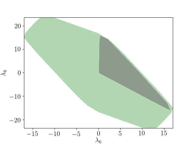
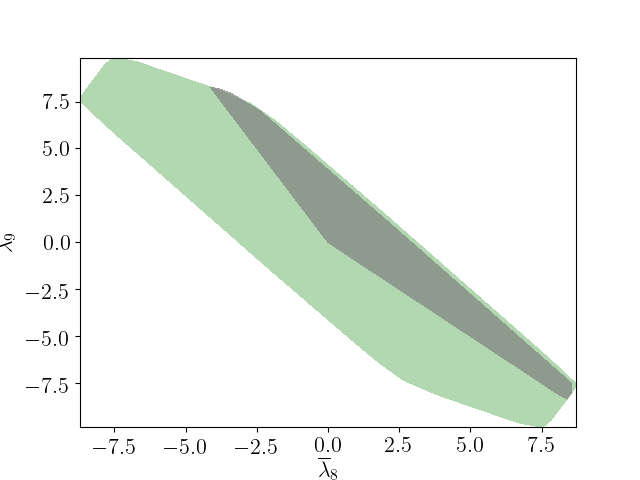
In order to validate our rough analytical understanding and to further explore the impact of the unitarity and BFB constraints we use the numerical machinery. There are many possibilities what to use as input parameters. Naively using the initial Lagrangian parameters will hardly produce points which are in agreement with the Higgs measurements. Therefore, we trade hybrid parameterization. With that choice, the full set of parameters is given by Eq. 58. As first step, we show in Fig. 1, all generated points in the planes λ6subscript𝜆6\lambda_{6} vs λ8subscript𝜆8\lambda_{8}, λ7subscript𝜆7\lambda_{7} vs λ9subscript𝜆9\lambda_{9} and λ¯8subscript¯𝜆8\bar{\lambda}_{8} vs λ¯9subscript¯𝜆9\bar{\lambda}_{9}.

Refer to caption
Refer to caption
Refer to caption
Figure 1: The allowed ranges of (λ6,λ8)subscript𝜆6subscript𝜆8(\lambda_{6},\lambda_{8}) (left), (λ7,λ9)subscript𝜆7subscript𝜆9(\lambda_{7},\lambda_{9}) (middle) and (λ¯8,λ¯9)subscript¯𝜆8subscript¯𝜆9(\bar{\lambda}_{8},\bar{\lambda}_{9}) (right) by imposing unitarity (green), combined unitarity and BFB (grey) constraints.

In the 2HDMcT, the presence of the triplet field implies a new scalar couplings λ6,7,8,9subscript𝜆6789\lambda_{6,7,8,9} et λ¯8,9subscript¯𝜆89\bar{\lambda}_{8,9} and the vacuum stability condition requires that not only λ1,20subscript𝜆120\lambda_{1,2}\geq 0 but also λ7,80subscript𝜆780\lambda_{7,8}\geq 0 with the conditions in Eq. (71). By varying λ1,5subscript𝜆15\lambda_{1,...5} in [8π:8π]delimited-[]:8𝜋8𝜋[-8\pi:8\pi], we show in Fig. 1, the allowed domains on λ6,7,8,9subscript𝜆6789\lambda_{6,7,8,9} et λ¯8,9subscript¯𝜆89\bar{\lambda}_{8,9} plans without conflicting with the theoretical constraints. We assume that the seesaw mechanism at the TeV scale that we consider here, is a ”low-energy” effective phenomenological manifestation at high energy scale. We therefore assume that the couplings remain perturbative up to GUT scale.

IV Limits from experimental constraints

IV.1 Oblic parameters

Strong indirect probe of physics beyond SM is provided by the oblique parameters S, T and U. More than that, the calculations of several observables check their dependences on those oblique parameters, for example, and not as a limitation, the ρ𝜌\rho parameter veltman75 , i.e. ρ=mW2/mZ2cW2𝜌superscriptsubscript𝑚𝑊2superscriptsubscript𝑚𝑍2superscriptsubscript𝑐𝑊2\rho=m_{W}^{2}/m_{Z}^{2}c_{W}^{2}. In the SM, this parameter is equal to 1 at tree level. In the THDMcT, the new triplet contributions to W𝑊W and Z𝑍Z masses readily form Eq. 26 and the kinetic terms in Eq. 8 leads to write,

mZ2=g2(v12+v22+4vt2)4cos2θWsuperscriptsubscript𝑚𝑍2superscript𝑔2superscriptsubscript𝑣12superscriptsubscript𝑣224superscriptsubscript𝑣𝑡24superscript2subscript𝜃𝑊\displaystyle m_{Z}^{2}=\frac{g^{2}\,(v_{1}^{2}+v_{2}^{2}+4v_{t}^{2})}{4\,\cos^{2}\theta_{W}} (72)
mW2=g2(v12+v22+2vt2)4=g2v24superscriptsubscript𝑚𝑊2superscript𝑔2superscriptsubscript𝑣12superscriptsubscript𝑣222superscriptsubscript𝑣𝑡24superscript𝑔2superscript𝑣24\displaystyle m_{W}^{2}=\frac{g^{2}\,(v_{1}^{2}+v_{2}^{2}+2v_{t}^{2})}{4}=\frac{g^{2}\,v^{2}}{4} (73)

the modified form of the ρ𝜌\rho parameter reads

ρ=v02+2vt2v02+4vt212vt2v02=1+δρ0𝜌superscriptsubscript𝑣022superscriptsubscript𝑣𝑡2superscriptsubscript𝑣024superscriptsubscript𝑣𝑡212superscriptsubscript𝑣𝑡2superscriptsubscript𝑣021𝛿𝜌0\displaystyle\rho=\frac{v_{0}^{2}+2v_{t}^{2}}{v_{0}^{2}+4v_{t}^{2}}\approx 1-2\frac{v_{t}^{2}}{v_{0}^{2}}=1+\delta\rho\neq 0 (74)

The impact of a 2HDMcT in the so-called electroweak precision requires that ρ𝜌\rho to be close to its SM value: ρ=1.00040.0004+0.0003𝜌subscriptsuperscript1.00040.00030.0004\rho=1.0004^{+0.0003}_{-0.0004} pdg2016 . Then, one gets an upper bound for vt<5subscript𝑣𝑡5v_{t}<5 GeV. Furthermore, the major contribution to the T-parameter comes from the loops involving the scalar triplet when vtsubscript𝑣𝑡v_{t} equal to zero or less. Also, since deviations from the Standard Model expectations in U𝑈U are negligible negU , then we will assume the latter to be zero and consider only S𝑆S and T𝑇T. We compute their χST2subscriptsuperscript𝜒2𝑆𝑇\chi^{2}_{ST} contribution through,

χST2=(SSbestTTbest)(0.00850.00630.00630.0057)1(SSbestTTbest)subscriptsuperscript𝜒2𝑆𝑇𝑆superscript𝑆𝑏𝑒𝑠𝑡𝑇superscript𝑇𝑏𝑒𝑠𝑡superscript0.00850.00630.00630.00571𝑆superscript𝑆𝑏𝑒𝑠𝑡𝑇superscript𝑇𝑏𝑒𝑠𝑡\displaystyle\chi^{2}_{ST}=\left(\begin{array}[]{cc}S-S^{best}&T-T^{best}\end{array}\right)\left(\begin{array}[]{cc}0.0085&0.0063\\ 0.0063&0.0057\end{array}\right)^{-1}\left(\begin{array}[]{c}S-S^{best}\\ T-T^{best}\end{array}\right) (80)

For U=0𝑈0U=0,the electroweak fit gives the values.

Sbest=0.06,Tbest=0.097\displaystyle S^{best}=0.06\;\;\;\;\;\;,\;\;\;\;\;T^{best}=0.097 (81)

The contribution of the scalar triplet to S𝑆S and T𝑇T reads as sharma2012

T=T2HDMcT=14πsw2mW2[+F(m++2,m+2)++, 0F(m+2,m02)]TsubscriptT2𝐻𝐷𝑀𝑐𝑇14𝜋subscriptsuperscript𝑠2𝑤subscriptsuperscript𝑚2𝑊delimited-[]subscript𝐹superscriptsubscript𝑚absent2superscriptsubscript𝑚2subscript 0𝐹superscriptsubscript𝑚2superscriptsubscript𝑚02\displaystyle\text{T}=\text{T}_{2HDMcT}=\frac{1}{4\pi s^{2}_{w}m^{2}_{W}}\bigg{[}\sum_{+}F(m_{++}^{2},m_{+}^{2})+\sum_{+,\,0}F(m_{+}^{2},m_{0}^{2})\bigg{]} (82)
S=S2HDMcT=13π[0log(m++2m02)+60ξ(m02mZ2,m02mZ2)+6(12sw2)2ξ(m++2mZ2,m++2mZ2)\displaystyle\text{S}=\text{S}_{2HDMcT}=-\frac{1}{3\pi}\bigg{[}\sum_{0}\log\left(\frac{m_{++}^{2}}{m_{0}^{2}}\right)+6\sum_{0}\xi\left(\frac{m_{0}^{2}}{m_{Z}^{2}},\frac{m_{0}^{2}}{m_{Z}^{2}}\right)+6(1-2s^{2}_{w})^{2}\xi\left(\frac{m_{++}^{2}}{m_{Z}^{2}},\frac{m_{++}^{2}}{m_{Z}^{2}}\right)
+6sw4+ξ(m+2mZ2,m+2mZ2)]\displaystyle\hskip 17.07182pt+6s^{4}_{w}\sum_{+}\xi\left(\frac{m_{+}^{2}}{m_{Z}^{2}},\frac{m_{+}^{2}}{m_{Z}^{2}}\right)\bigg{]} (83)

where, m++=mH±±subscript𝑚absentsubscript𝑚superscript𝐻plus-or-minusabsentplus-or-minusm_{++}=m_{H^{\pm\pm}}, m+=mH1±,mH2±subscript𝑚subscript𝑚superscriptsubscript𝐻1plus-or-minussubscript𝑚superscriptsubscript𝐻2plus-or-minusm_{+}=m_{H_{1}^{\pm}},m_{H_{2}^{\pm}} and m0=mh2,mh3subscript𝑚0subscript𝑚subscript2subscript𝑚subscript3m_{0}=m_{h_{2}},m_{h_{3}}, while swsubscript𝑠𝑤s_{w} stands for the sinus of the Weinberg angle θwsubscript𝜃𝑤\theta_{w}. The function ξ(x,y)𝜉𝑥𝑦\xi(x,y) and F(x,y)𝐹𝑥𝑦F(x,y) are defined by,

F(x,y)=x+y2xyxyln(xy)𝐹𝑥𝑦𝑥𝑦2𝑥𝑦𝑥𝑦𝑥𝑦\displaystyle F(x,y)=\frac{x+y}{2}-\frac{xy}{x-y}\ln\left(\frac{x}{y}\right) (84)
ξ(x,y)𝜉𝑥𝑦\displaystyle\xi(x,y) =\displaystyle= 49512(x+y)+16(xy)2+14[x2y213(xy)3x2+y2xy]lnxy49512𝑥𝑦16superscript𝑥𝑦214delimited-[]superscript𝑥2superscript𝑦213superscript𝑥𝑦3superscript𝑥2superscript𝑦2𝑥𝑦𝑥𝑦\displaystyle\frac{4}{9}-\frac{5}{12}\left(x+y\right)+\frac{1}{6}\left(x-y\right)^{2}+\frac{1}{4}\Big{[}x^{2}-y^{2}-\frac{1}{3}\left(x-y\right)^{3}-\frac{x^{2}+y^{2}}{x-y}\Big{]}\ln\frac{x}{y} (85)
\displaystyle- 112d(x,y)f(x,y)112𝑑𝑥𝑦𝑓𝑥𝑦\displaystyle\frac{1}{12}d\left(x,y\right)f\left(x,y\right)
f(x,y)={2d(x,y)[arctanxy+1d(x,y)arctanxy1d(x,y)ford(x,y)>00ford(x,y)=0d(x,y)ln[x+y1+d(x,y)x+y1d(x,y)]ford(x,y)<0\displaystyle f\left(x,y\right)=\left\{\begin{matrix}-2\sqrt{d\left(x,y\right)}\Big{[}\arctan\frac{x-y+1}{\sqrt{d\left(x,y\right)}}-\arctan\frac{x-y-1}{\sqrt{d\left(x,y\right)}}&for&d\left(x,y\right)>0\\ 0&for&d\left(x,y\right)=0\\ \sqrt{-d\left(x,y\right)}\ln\Big{[}\frac{x+y-1+\sqrt{-d\left(x,y\right)}}{x+y-1-\sqrt{-d\left(x,y\right)}}\Big{]}&for&d\left(x,y\right)<0\end{matrix}\right. (86)
d(x,y)=1+2(x+y)(xy)2𝑑𝑥𝑦12𝑥𝑦superscript𝑥𝑦2\displaystyle d\left(x,y\right)=-1+2\left(x+y\right)-\left(x-y\right)^{2} (87)

IV.2 Direct LHC and LEP constraints

The HiggsBounds code HiggsBounds is used to test a model against experimental data from LEP, Tevatron and the LHC. In our analysis we use part function of HiggsBounds version 5.2.0beta5.2.0𝑏𝑒𝑡𝑎5.2.0beta with the latest constraints for heavy Higgs bosons. The required input for HiggsBounds program are masses for all the scalar, the effective Higgs couplings, the total decay widths for all scalar and the branching ratios. The exclusion test at 2σ2𝜎2\sigma is then performed on the five physical scalars of our model. HiggsBounds returns a binary result indicating if the specific model point has been excluded at 95%percent\% C.L. or not.

Both experiments ATLAS and CMS at LHC reported the discovery of a scalar particule with mass around 125.09 GeV masse_higgs . Meanwhile, this has been strengthen further by ATLAS and CMS with the first 13 TeV results. In our model, we identify the Higgs field H1subscript𝐻1H_{1} with the observed SM-like Higgs boson with a mass:

mh1=125.09±0.4GeVsubscript𝑚subscript1plus-or-minus125.090.4GeV\displaystyle m_{h_{1}}=125.09\pm 0.4\,\text{GeV} (88)

We include both the measured signal rates from the ATLAS and CMS Run I and Run II and their combinaisons in our study via the public code HiggsSignals-2.2.1beta HiggsSignals .

The global χ𝜒\chi-square is defined by:

χ2=χHS2(8TeV)+χHS2( 13TeV)+χST2superscript𝜒2subscriptsuperscript𝜒28𝑇𝑒𝑉𝐻𝑆subscriptsuperscript𝜒213𝑇𝑒𝑉𝐻𝑆subscriptsuperscript𝜒2𝑆𝑇\displaystyle\chi^{2}=\chi^{2\,(8\,TeV)}_{HS}+\chi^{2\,(\,13TeV)}_{HS}+\chi^{2}_{ST} (89)

we then determine the minimal χ2superscript𝜒2\chi^{2} value over the scanned parameter space, χmin2subscriptsuperscript𝜒2𝑚𝑖𝑛\chi^{2}_{min}, and keep the allowed parameter space that features a χ2superscript𝜒2\chi^{2} value within Δχ2=χ2χmin22.3, 5.99, 11.8formulae-sequenceΔsuperscript𝜒2superscript𝜒2subscriptsuperscript𝜒2𝑚𝑖𝑛2.35.9911.8\Delta\chi^{2}=\chi^{2}-\chi^{2}_{min}\leq 2.3,\,5.99,\,11.8 (which corresponds respectively to 68%percent\% CL, 95.5%percent\% CL and 99.7%percent\% CL.)

V Light and heavy Higgs Phenomenology

In this section we study the influence of the constraints presented in the previous section (indirect, LEP, Tevatron and LHC constraints) on the free parameters. For this purpose we generate a set of 109superscript10910^{9} points randomly for each of the two different types of model defined in Tables 1 and 2 with random values for each of the free parameters. The available ranges we use in the simulation are given:

mh1mh2mh31TeV,  80GeVmH±±1TeV,π2α1,2,3π21tanβ40,102μ1102,vt=1GeV,λ10.15,λ31.6,λ41.6matrixformulae-sequencesubscript𝑚subscript1subscript𝑚subscript2subscript𝑚subscript31TeV80GeVsubscript𝑚superscript𝐻plus-or-minusabsentplus-or-minus1TeV𝜋2subscript𝛼123𝜋2formulae-sequence1𝛽40superscript102subscript𝜇1superscript102formulae-sequencesubscript𝑣𝑡1GeVformulae-sequencesubscript𝜆10.15formulae-sequencesubscript𝜆31.6subscript𝜆41.6\displaystyle\begin{matrix}m_{h_{1}}\leq m_{h_{2}}\leq m_{h_{3}}\leq 1\,\text{TeV},\,\,80\,\text{GeV}\leq m_{H^{\pm\pm}}\leq 1\,\text{TeV},\,\,\\ \frac{-\pi}{2}\leq\alpha_{1,2,3}\leq\frac{\pi}{2}\\ 1\leq\tan\beta\leq 40,\,\,-10^{2}\leq\mu_{1}\leq 10^{2},\,\,v_{t}=1\,\text{GeV},\,\,\,\lambda_{1}\approx 0.15,\,\,\lambda_{3}\approx 1.6,\,\,\lambda_{4}\approx 1.6\end{matrix} (90)

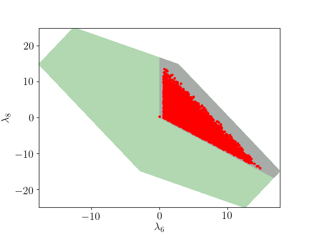
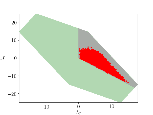
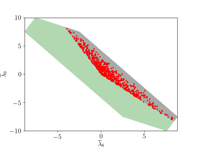
λ1subscript𝜆1\lambda_{1}, λ3subscript𝜆3\lambda_{3} and λ4subscript𝜆4\lambda_{4} are set respectively to the values 0.150.150.15, 1.61.61.6 and 1.61.61.6 for the sake of simplification. The ranges for λ6subscript𝜆6\lambda_{6}, λ7subscript𝜆7\lambda_{7}, λ8subscript𝜆8\lambda_{8}, λ9subscript𝜆9\lambda_{9}, λ¯8subscript¯𝜆8\bar{\lambda}_{8} and λ¯9subscript¯𝜆9\bar{\lambda}_{9} resulted from the unitarity and boundedness constraints as can be seen from Fig. 2. For simplicity, let us classify the dimensionless parameters in the scalar potential into two different sets according to the following two types of constraints:

  • First set of constraints includes the unitarity, vacuum stability and BFB constraints as well as non-tachyonic masses. We refer to this set as C1subscript𝐶1C_{1}.

  • The second set of constraints contains C1subscript𝐶1C_{1} and constraints from Higgs data. We refer to this set as C2subscript𝐶2C_{2}.

Refer to caption
Refer to caption
Refer to caption
Figure 2: The largest (λ6,λ8)subscript𝜆6subscript𝜆8(\lambda_{6},\lambda_{8}) (left), (λ7,λ8)subscript𝜆7subscript𝜆8(\lambda_{7},\lambda_{8}) (center) and (λ¯8,λ¯9)subscript¯𝜆8subscript¯𝜆9(\bar{\lambda}_{8},\bar{\lambda}_{9}) (right) domain allowed by C1subscript𝐶1C_{1} (gray) and C2subscript𝐶2C_{2} (red)

In Fig. 2, all the generated points are plotted in the planes λ6subscript𝜆6\lambda_{6} vs λ8subscript𝜆8\lambda_{8}, λ7subscript𝜆7\lambda_{7} vs λ9subscript𝜆9\lambda_{9} and λ¯8subscript¯𝜆8\bar{\lambda}_{8} vs λ¯9subscript¯𝜆9\bar{\lambda}_{9}, as we can see C2subscript𝐶2C_{2} set of constraints reduce the above domain of λ6subscript𝜆6\lambda_{6}, λ7subscript𝜆7\lambda_{7}, λ8subscript𝜆8\lambda_{8}, λ9subscript𝜆9\lambda_{9}, λ¯8subscript¯𝜆8\bar{\lambda}_{8} and λ¯9subscript¯𝜆9\bar{\lambda}_{9}.

Looking now at the plane λ¯8subscript¯𝜆8\bar{\lambda}_{8} vs λ¯9subscript¯𝜆9\bar{\lambda}_{9} are not very much restricted by C2subscript𝐶2C_{2} constraint due to the fact that λ¯8subscript¯𝜆8\bar{\lambda}_{8} and λ¯9subscript¯𝜆9\bar{\lambda}_{9} are always dependent of the vev of scalar triplet.

In Fig. 3, we present the allowed points in the (sign(CVh1)sin(α1π/2),tanβ)signsuperscriptsubscriptCVsubscripth1subscript𝛼1𝜋2𝛽(\rm{sign}(C_{V}^{h_{1}})\sin(\alpha_{1}-\pi/2)\,,\,\tan\beta) plane, that passes all constraints in type II (left) and type I (right) at 1σ1𝜎1\sigma, 2σ2𝜎2\sigma and 3σ3𝜎3\sigma. In type-II, one can appreciate that the mixing angle α1subscript𝛼1\alpha_{1} seems more constrained than in type-I. Results are shown by imposing the conditions C1subscript𝐶1C_{1} and C2subscript𝐶2C_{2}. The later has a strong impact on how the mixing angles are constrained. Fig.3(left) displays wrong-sing Yukawa couplings scenario at 2σ𝜎\sigma.

Refer to caption
Refer to caption
Figure 3: The allowed regions in (sgn(CVh1)sin(α1π/2)𝑠𝑔𝑛superscriptsubscript𝐶𝑉subscript1subscript𝛼1𝜋2sgn(C_{V}^{h_{1}})\sin(\alpha_{1}-\pi/2), tanβ𝛽\tan\beta) after imposing C1subscript𝐶1C_{1} and C2subscript𝐶2C_{2} constraints, where the left and right panels represent the allowed values in type-II(left), type-I(right), respectively. The errors for χ𝜒\chi-square fit are 99.7% CL (red), 95.5% CL (blue) and 68% CL (yellow).

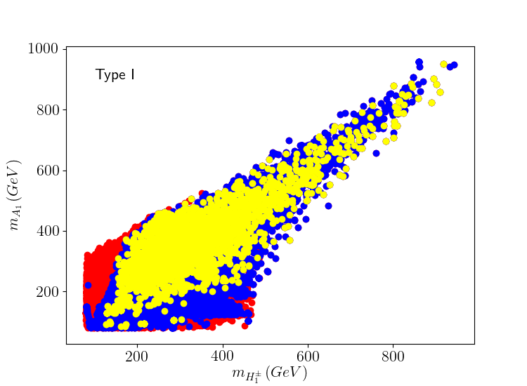
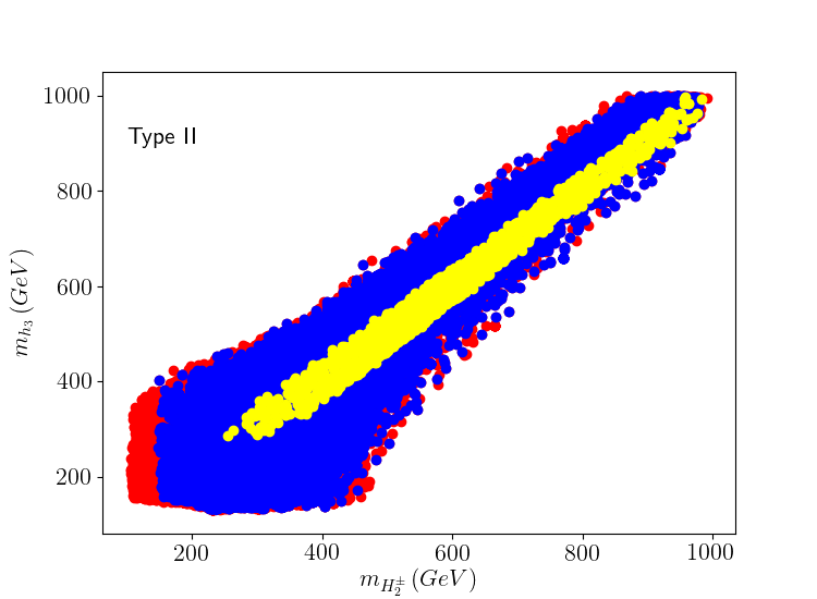
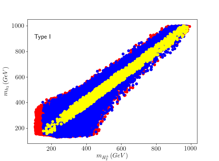
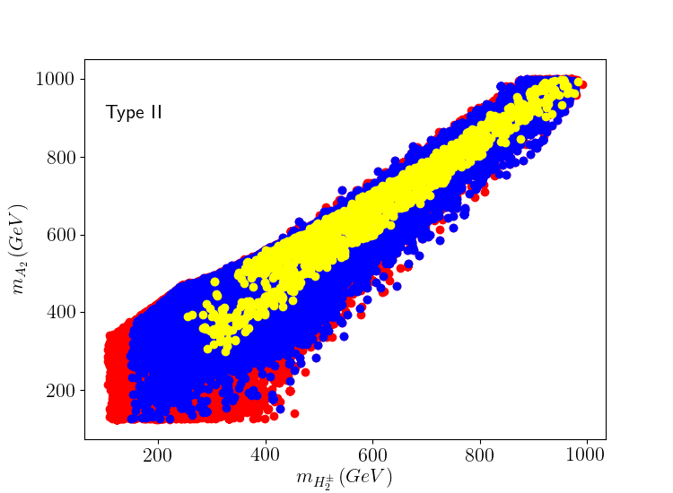
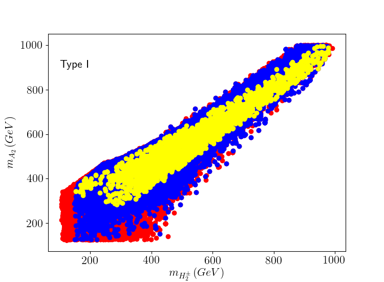
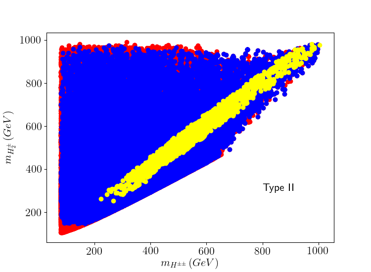
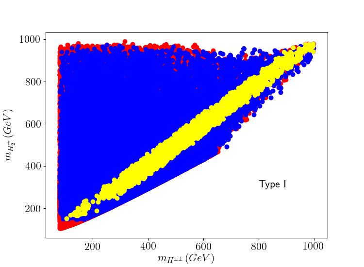
In Fig. 4, the allowed ranges are plotted in the planes mA1subscript𝑚subscript𝐴1m_{A_{1}}, mA2subscript𝑚subscript𝐴2m_{A_{2}}, mh3subscript𝑚subscript3m_{h_{3}} and mH±±subscript𝑚superscript𝐻plus-or-minusabsentplus-or-minusm_{H^{\pm\pm}} vs mH2±subscript𝑚subscriptsuperscript𝐻plus-or-minus2m_{H^{\pm}_{2}}. The left-columns panels corresponds to type-II, the right-column to the type-I, all points passed the constraints mentioned above at 1σ𝜎\sigma (yellow), 2σ𝜎\sigma (blue) and 3σ𝜎\sigma (red). As can be seeing most of the masses can be light in type-I less than 300 GeV.
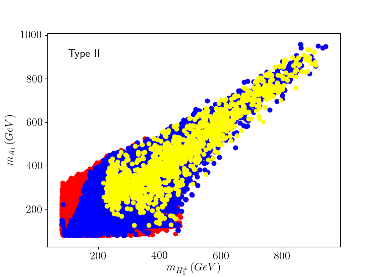
Refer to caption
Refer to caption
Refer to caption
Refer to caption
Refer to caption
Refer to caption
Refer to caption
Refer to caption
Figure 4: Allowed mass ranges in 2HDMcT type-II (left column) and type-I (right column) taking into account all theoretical and experimental constraints.

Looking only at the yellow points, those which pass the C2subscript𝐶2C_{2} constraint, we can see that the mA2subscript𝑚subscript𝐴2m_{A_{2}}, mH2±subscript𝑚subscriptsuperscript𝐻plus-or-minus2m_{H^{\pm}_{2}}, mh3subscript𝑚subscript3m_{h_{3}} and mH±±subscript𝑚superscript𝐻plus-or-minusabsentplus-or-minusm_{H^{\pm\pm}} masses are bounded in type II where we find that most of the yellow points lie in the ranges mH1±,H2±,A1,A2,h2,h3,H±±[200,1000]subscript𝑚superscriptsubscript𝐻1plus-or-minussuperscriptsubscript𝐻2plus-or-minussubscript𝐴1subscript𝐴2subscript2subscript3superscript𝐻plus-or-minusabsentplus-or-minus2001000m_{H_{1}^{\pm},H_{2}^{\pm},A_{1},A_{2},h_{2},h_{3},H^{\pm\pm}}\in[200,1000] GeV.

The sensitivity of the Higgs couplings of h1subscript1h_{1} at the LHC is not appreciably better than 20%percent\%, leaving thus a significant window of opportunity for new physics. Here we investigate the correlations among relevant couplings within the C1𝐶1C1 and C2subscript𝐶2C_{2} constraints. In Fig 5, we show these correlations which are consistent within the BRs of mh1=125subscript𝑚subscript1125m_{h_{1}}=125 GeV within 1σ𝜎\sigma (yellow) and 2σ𝜎\sigma(blue). This is related to the fact that the central values of some Higgs couplings deviate from the SM, which strongly restrict the range of deviations from the SM. While the decay h1Zγsubscript1𝑍𝛾h_{1}\to Z\gamma is not yet observed at the LHC, the correlation between the h1WW,γγsubscript1𝑊𝑊𝛾𝛾h_{1}\to WW,\gamma\gamma and hbb¯𝑏¯𝑏h\to b\bar{b} couplings can now be measured by the experiments. The ratio of the BR of WW𝑊𝑊WW to that γγ𝛾𝛾\gamma\gamma can be measured with an accuracy better than 5%percent\% and an integrated luminosity that is expected to be accumulated by the High Luminosity LHC.

Refer to caption
Refer to caption
Refer to caption
Refer to caption
Figure 5: Correlation plots between the BRs of (a) h1WWsubscript1𝑊𝑊h_{1}\to WW vs h1γγsubscript1𝛾𝛾h_{1}\to\gamma\gamma, (b) h1WWsubscript1𝑊𝑊h_{1}\to WW vs h1bb¯subscript1𝑏¯𝑏h_{1}\to b\bar{b}, (c) h1ττsubscript1𝜏𝜏h_{1}\to\tau\tau vs h1γγsubscript1𝛾𝛾h_{1}\to\gamma\gamma and (d) h1γγsubscript1𝛾𝛾h_{1}\to\gamma\gamma vs h1h1Zγsubscript1subscript1𝑍𝛾h_{1}\to h_{1}\to Z\gamma in 2HDMcT type-II by considering the BRs of the lightest h1subscript1h_{1} boson consistent within 95.5% CL (blue) and 68% CL (yellow)

In the following, we will scrutinize the impact of the searches for heavy Higgs particles in 2HDMcT ordered by their decay products. First we will address the bosonic decays to VV𝑉𝑉VV (V=γ,Z,W±𝑉𝛾𝑍superscript𝑊plus-or-minusV=\gamma,Z,W^{\pm}) and fermionic mode ττ+superscript𝜏superscript𝜏\tau^{-}\tau^{+} branching ratios of the neutral Higgs (h2subscript2h_{2}, h3subscript3h_{3}, A1subscript𝐴1A_{1} and A2subscript𝐴2A_{2}) using both CMS and ATLAS Higgs data for 8 TeV ATLAS1 ; ATLAS2 ; ATLAS3 and 13 TeV ATLAS4 ; ATLAS5 ; ATLAS6 ; ATLAS7 ; ATLAS88 . After that, we will turn towards the pair production of hihjsubscript𝑖subscript𝑗h_{i}h_{j}. The narrow width approximation will be applied throughout this section, we will comment on its validity at the end of the text section. We define the cross section as,

σ2HDMcT(ppϕ)=kg2σSM(ppϕ),ϕ=h2,3orA1,2formulae-sequencesuperscript𝜎2𝐻𝐷𝑀𝑐𝑇𝑝𝑝italic-ϕsubscriptsuperscript𝑘2𝑔superscript𝜎𝑆𝑀𝑝𝑝italic-ϕitalic-ϕsubscript23𝑜𝑟subscript𝐴12\displaystyle\sigma^{2HDMcT}(pp\rightarrow\phi)=k^{2}_{g}\sigma^{SM}(pp\rightarrow\phi),\,\,\ \phi=h_{2,3}\,\,or\,\,A_{1,2} (91)

where σSM(ggϕ)superscript𝜎𝑆𝑀𝑔𝑔italic-ϕ\sigma^{SM}(gg\rightarrow\phi) is the cross section for Higgs production in gluon fusion in the SM, and kg2=Γ2HDMcT(ϕgg)/ΓSM(ϕgg)subscriptsuperscript𝑘2𝑔subscriptΓ2𝐻𝐷𝑀𝑐𝑇italic-ϕ𝑔𝑔subscriptΓ𝑆𝑀italic-ϕ𝑔𝑔k^{2}_{g}=\Gamma_{2HDMcT}(\phi\rightarrow gg)/\Gamma_{SM}(\phi\rightarrow gg), with Γ2HDMcT(ϕgg)subscriptΓ2𝐻𝐷𝑀𝑐𝑇italic-ϕ𝑔𝑔\Gamma_{2HDMcT}(\phi\rightarrow gg) and ΓSM(ϕgg)subscriptΓ𝑆𝑀italic-ϕ𝑔𝑔\Gamma_{SM}(\phi\rightarrow gg) are the partial decay rates in 2HDMcT and SM respectively.

h2,3ZZsubscript23𝑍𝑍h_{2,3}\to ZZ and WW𝑊𝑊WW

We use Sushi v1.6.0 public code Sushi1 ; Sushi2 at NNLO QCD to perform the calculation of the cross sections for Higgs production in gluon fusion (ggF)𝑔𝑔𝐹(ggF) and bottom-quark annihilation in the SM at 13 TeV. The relative coupling of h2,3subscript23h_{2,3} to the two vector bosons ZZ𝑍𝑍ZZ and WW𝑊𝑊WW is universal and type independent. However, the production of the h2,3subscript23h_{2,3} differs between the types. In Fig. (6) we plot the production cross sections in proton proton fusion times ZZ𝑍𝑍ZZ and WW𝑊𝑊WW branching ratios of h2,3subscript23h_{2,3} Higgs after imposing C1subscript𝐶1C_{1} and C2subscript𝐶2C_{2} constrains within 99.7% CL (red), 95.5% CL (blue) and 68% CL(yellow) of the Higgs data. It is well seeing from Fig. (6) that h2,3WW/ZZsubscript23𝑊𝑊𝑍𝑍h_{2,3}\to WW/ZZ rates are compared to what would be expected at Run-II LHC. The colored lines in Fig. (6) denote the observed limits in ZZ/WW𝑍𝑍𝑊𝑊ZZ/WW final states from 13 TeV ATLAS data ATLAS10 ; ATLAS11 ; ATLAS12 ; ATLAS13 . The direct LHC searches for this channels yield a strong suppression of σ×BR𝜎𝐵𝑅\sigma\times BR. For ZZ𝑍𝑍ZZ searches the mh2250subscript𝑚subscript2250m_{h_{2}}\leq 250 GeV region is constrained by Run-I data whereas Run-II data determine the dominant limits for the rest of the mass region. For the WW𝑊𝑊WW searches, Run-I data dictate the limit until 350 GeV and the high mass range is dominated by Run-II data.
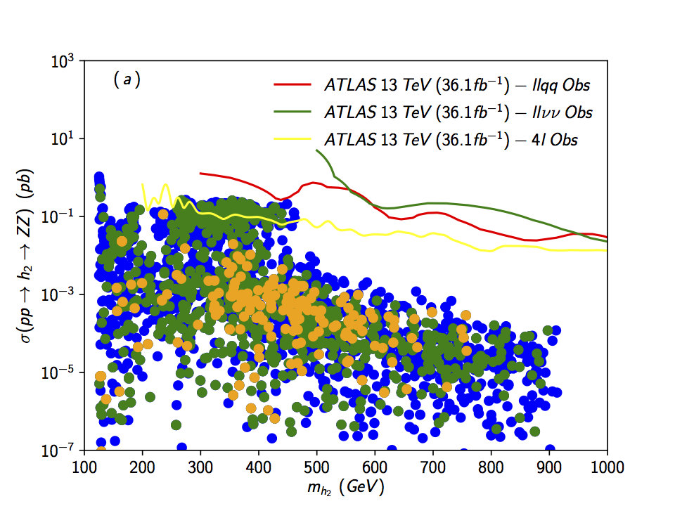
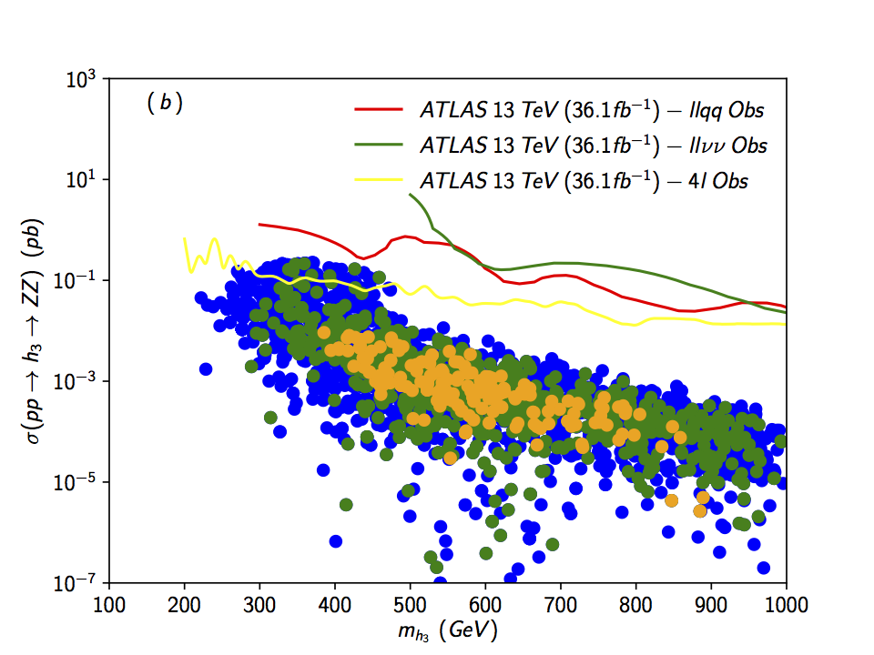
Refer to caption
Refer to caption
Refer to caption
Refer to caption
Figure 6: Scatter plot for σ(pph2,3)×Br(h2,3ZZ,WW)𝜎𝑝𝑝subscript23𝐵𝑟subscript23𝑍𝑍𝑊𝑊\sigma(pp\to h_{2,3})\times Br(h_{2,3}\to ZZ,WW) as a function mh2,3subscript𝑚subscript23m_{h_{2,3}} after imposing C1subscript𝐶1C_{1} and C2subscript𝐶2C_{2} constrains assuming 99.7% CL (red), 95.5% CL (blue) and 68% CL (yellow) in 2HDMcT type-II

h2,3,A1,2γγsubscript23subscript𝐴12𝛾𝛾h_{2,3},A_{1,2}\to\gamma\gamma

Direct searches for a heavy Higgs decaying to two photons constrain σ×BR𝜎𝐵𝑅\sigma\times BR by roughly one magnitude compared the ATLAS limit in CP-even decay modes (see Fig. 7). The searches in the di-photon decay channel of a pseudoscalar Higgs yield a suppression of σ×BR𝜎𝐵𝑅\sigma\times BR one to three orders of magnitude compared to the ATLAS limit for mA1,2400subscript𝑚subscript𝐴12400m_{A_{1,2}}\leq 400 GeV certain intermediate σ×BR𝜎𝐵𝑅\sigma\times BR regions for low mA1,2subscript𝑚subscript𝐴12m_{A_{1,2}} are disfavoured by the prior.
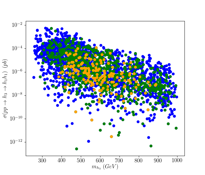
Refer to caption
Refer to caption
Refer to caption
Refer to caption
Figure 7: Scatter plot in the mϕsubscript𝑚italic-ϕm_{\phi}-[σ×Br(ϕγγ)]delimited-[]𝜎𝐵𝑟italic-ϕ𝛾𝛾[\sigma\times Br(\phi\rightarrow\gamma\gamma)] (ϕ=h2,3italic-ϕsubscript23\phi=h_{2,3} or A2,3subscript𝐴23A_{2,3}) planes after imposing C3subscript𝐶3C_{3} constrains at s=13𝑠13\sqrt{s}=13 TeV. The errors for χ𝜒\chi-square fit are 99.7% CL (red), 95.5% CL (blue) and 68% CL (yellow) in 2HDMcT type-II.
Refer to caption
Refer to caption
Refer to caption
Refer to caption
Figure 8: The same as Fig. (7) but for ττ𝜏𝜏\tau\tau pair production at s=13𝑠13\sqrt{s}=13 TeV in 2HDMcT type-II
Refer to caption
Refer to caption
Refer to caption
Refer to caption
Figure 9: The same as Fig. (7) but for hihjsubscript𝑖subscript𝑗h_{i}h_{j} pair production at s=13𝑠13\sqrt{s}=13 TeV in 2HDMcT type-II

In Fig. 8 we plot the production cross section in proton proton fusion times ττ𝜏𝜏\tau\tau branching ration after imposing C3subscript𝐶3C_{3} constrains. The errors for χ𝜒\chi-square fit are 99.7% CL (red), 95.5% CL (blue) and 68% CL (yellow). The red(green) solid line in Fig. 8 is the upper limit on the cross-section times branching ration from the ATLAS𝐴𝑇𝐿𝐴𝑆ATLAS 13 TeV results ATLAS14 (CMS𝐶𝑀𝑆CMS 13 TeV results ATLAS15 ). The colored lines in Fig. 7 denote the observed limits from 13 TeV ATLAS data ATLAS16 .

h2,3hihjsubscript23subscript𝑖subscript𝑗h_{2,3}\to h_{i}h_{j} with (i,j)=(1,2)𝑖𝑗12(i,j)=(1,2)

Finally, in Fig. (9) we present a sample of points generated for Higgs pair production in the scenario where the observed Higgs boson is the lightest scalar h1subscript1h_{1} (top panels) and the next-to-lighest scalar (bottom panels). We present cross sections as a function of the masses of the two new scalars that can be involved in the chain decay contributions. We overlay three layers of point for which the total cross section is within 3σ3𝜎3\sigma (red), 2σ(blue)2𝜎𝑏𝑙𝑢𝑒2\sigma(blue) and 1σ1𝜎1\sigma respectively at the LHC Run-2. In the upper plots, where h1subscript1h_{1} chain decays become possible above 250 GeV. In Fig.(9) at nearly mh1mh2similar-tosubscript𝑚subscript1subscript𝑚subscript2m_{h_{1}}\sim m_{h_{2}}, which means that some opening decay channels contribute to chain decay h3h1+h1,h1+h2subscript3subscript1subscript1subscript1subscript2h_{3}\to h_{1}+h_{1},h_{1}+h_{2} and h2+h2subscript2subscript2h_{2}+h_{2}. This means that imposing a constraint on the parameter space with including the chain decay contribution would be too strong at the LHC Run-2. Overall, the shape of the three different σ𝜎\sigma regions in the various panels is the results of an interplay between the kinematics and the applied constraints. To certain extent the structure can be directly related to the exclusion curves from the collider searches imposed by HiggsBound. The strong increase at mh3=250subscript𝑚subscript3250m_{h_{3}}=250 GeV in the lower left panel is due the opening of the decay h3h2+h2subscript3subscript2subscript2h_{3}\to h_{2}+h_{2} and the decrease in the number of points for large values of mh3subscript𝑚subscript3m_{h_{3}} is due the S and T parameters.

VI Benchmark points for the LHC Run-2 in 2HDMcT

Benchmark points In this section we provide a set of benchmark points in 2HDMcT. There are chosen to cover various physical situations. From a phenomenological perspective we are interested in maximising various visibility of the new scalars in the LHC Run-2 and in covering, simultaneously, many kinematically different possibilities. In particular, we are interested in scenarios where hSM=h1subscript𝑆𝑀subscript1h_{SM}=h_{1}, hSM=h2subscript𝑆𝑀subscript2h_{SM}=h_{2} and hSM=h3subscript𝑆𝑀subscript3h_{SM}=h_{3} while preserving consistency with LHC Run-2 measurements. Thus, in many of the points presented below we have tried to maximise the cross section for the cross sections. At the same time we required the rates of the SM-like Higgs within 2σ2𝜎2\sigma from the global signal strength provided by the ATLAS and CMS data from LHC Run-2. Table (3), contains the parameters that define the chosen benchmark points and the production rate of the lightest as well as next-to-lightest Higgs bosons h2subscript2h_{2} and h3subscript3h_{3} in the various final states.

BP1 BP2 BP3 BP4 BP5
mh1subscript𝑚1m_{h1} (GeV) 125.1125.1125.1 125.1125.1125.1 12.75 77.27 21.8
mh2subscript𝑚subscript2m_{h_{2}} (GeV) 415.46 354.18 125.1125.1125.1 125.1125.1125.1 101.7
mh3subscript𝑚subscript3m_{h_{3}} (GeV) 426.17 937.02 155.96 448.59 125.1125.1125.1
mA1subscript𝑚subscript𝐴1m_{A_{1}} (GeV) 258.76 311.72 152.46 174.34 104
mA2subscript𝑚subscript𝐴2m_{A_{2}} (GeV) 417.81 936.06 270.28 457 327
mH1±subscript𝑚subscriptsuperscript𝐻plus-or-minus1m_{H^{\pm}_{1}} (GeV) 270.22 267.60 147.13 232.8 143
mH2±subscript𝑚subscriptsuperscript𝐻plus-or-minus2m_{H^{\pm}_{2}} (GeV) 386.35 906.42 164.24 434.7 174.87
mH±±subscript𝑚superscript𝐻plus-or-minusabsentplus-or-minusm_{H^{\pm\pm}} (GeV) 352.06 875.54 161.01 397.2 174.89
α1subscript𝛼1\alpha_{1} -1.26 -1.25 -0.46 -0.58 -0.08
α2subscript𝛼2\alpha_{2} -0.011 -0.086 -0.16 0.45 -0.06
α3subscript𝛼3\alpha_{3} -1.08 -0.12 -0.13 -0.08 -1.25
vtsubscript𝑣𝑡v_{t} (GeV) 1 1 1 1 1
λ6subscript𝜆6\lambda_{6} 5.56 0.89 6.24 4.17 5.92
λ7subscript𝜆7\lambda_{7} 1.13 0.69 5.52 4.57 7.08
λ8subscript𝜆8\lambda_{8} 2.75 1.54 -2.92 1.5 -4.64
λ9subscript𝜆9\lambda_{9} 1.50 3.36 0.90 -1.04 -0.6
tanβ𝛽\tan\beta 2.57 2.53 1.7 1.07 8.83
μ1subscript𝜇1\mu_{1} 26.22 16.42 -21.49 -36 56.69
μ2subscript𝜇2\mu_{2} 11.9 263.7 6.19 -451 1.19
μ3subscript𝜇3\mu_{3} -28.95 -615.2 3.41 525.42 -14.69
μh1subscript𝜇subscript1\mu_{h_{1}} 0.88 0.86 0.043 0.069 0.78
σ1σ(ggh1)subscript𝜎1𝜎𝑔𝑔subscript1\sigma_{1}\equiv\sigma(gg\rightarrow h_{1}) 132.9 [pb] 131.7 [pb] 10003.81 [pb] 175.45 [pb] 423.9[pb]
σ1×BR(h1WW)subscript𝜎1BRsubscript1𝑊𝑊\sigma_{1}\times{\rm BR}(h_{1}\rightarrow WW) 11.69 [pb] 10.70 [pb] 0 [fb] 0[fb] 0[pb]
σ1×BR(h1ZZ)subscript𝜎1BRsubscript1𝑍𝑍\sigma_{1}\times{\rm BR}(h_{1}\rightarrow ZZ) 1.73×10³absentsuperscript103\times 10^{3} [fb] 1.59×10³absentsuperscript103\times 10^{3}[fb] 0 [fb] 0 [fb] 0 [pb]
σ1×BR(h1bb)subscript𝜎1BRsubscript1𝑏𝑏\sigma_{1}\times{\rm BR}(h_{1}\rightarrow bb) 35.1 [pb] 35.96 [pb] 4811 [pb] 71.62 [pb] 177.45 [pb]
σ1×BR(h1ττ)subscript𝜎1BRsubscript1𝜏𝜏\sigma_{1}\times{\rm BR}(h_{1}\rightarrow\tau\tau) 4.24 [pb] 4.35[pb] 452×103absentsuperscript103\times 10^{3}[fb] 7.8×10³absentsuperscript103\times 10^{3} [fb] 17.7×10³absentsuperscript103\times 10^{3}[fb]
σ1×BR(h1γγ)subscript𝜎1BRsubscript1𝛾𝛾\sigma_{1}\times{\rm BR}(h_{1}\rightarrow\gamma\gamma) 0.12×10³absentsuperscript103\times 10^{3} [fb] 0.12×10³absentsuperscript103\times 10^{3}[fb] 7 [fb] 8.4 [fb] 0.34 [fb]
μh2subscript𝜇subscript2\mu_{h_{2}} 0.03 0.095 0.78 0.6 0.01
σ2σ(ggh2)subscript𝜎2𝜎𝑔𝑔subscript2\sigma_{2}\equiv\sigma(gg\rightarrow h_{2}) 0.53 [pb] 4.74 [pb] 106.18 [pb] 94.83 [pb] 18.31 [pb]
σ2×BR(h2WW)subscript𝜎2BRsubscript2𝑊𝑊\sigma_{2}\times{\rm BR}(h_{2}\rightarrow WW) 0.11 [pb] 0.56 [pb] 9.55×10³absentsuperscript103\times 10^{3}[fb] 11.4×10³absentsuperscript103\times 10^{3} [fb] 4.98×10³absentsuperscript103\times 10^{-3}[pb]
σ2×BR(h2ZZ)subscript𝜎2BRsubscript2𝑍𝑍\sigma_{2}\times{\rm BR}(h_{2}\rightarrow ZZ) 52 [fb] 260[fb] 1.41×10³absentsuperscript103\times 10^{3}[fb] 1.69×10³absentsuperscript103\times 10^{3} [fb] 9.66×10⁵absentsuperscript105\times 10^{-5} [pb]
σ2×BR(h2bb)subscript𝜎2BRsubscript2𝑏𝑏\sigma_{2}\times{\rm BR}(h_{2}\rightarrow bb) 6.2×10⁴absentsuperscript104\times 10^{-4} [pb] 4.1×10³absentsuperscript103\times 10^{-3}[pb] 19.06[pb] 23.12 [pb] 0.35[pb]
σ2×BR(h2ττ)subscript𝜎2BRsubscript2𝜏𝜏\sigma_{2}\times{\rm BR}(h_{2}\rightarrow\tau\tau) 9.38×10⁵absentsuperscript105\times 10^{-5} [pb] 6.1×10⁴absentsuperscript104\times 10^{-4}[pb] 2.3 ×10³absentsuperscript103\times 10^{3}[fb] 2.79×10³absentsuperscript103\times 10^{3} [fb] 0.041×10³absentsuperscript103\times 10^{3}[fb]
σ2×BR(h2γγ)subscript𝜎2BRsubscript2𝛾𝛾\sigma_{2}\times{\rm BR}(h_{2}\rightarrow\gamma\gamma) 7.401×10⁴absentsuperscript104\times 10^{-4} [fb] 7.86×10³absentsuperscript103\times 10^{-3}[fb] 0.1×10³absentsuperscript103\times 10^{3} [fb] 0.08×10³absentsuperscript103\times 10^{3} [fb] 1.86 [fb]
BR(h2h1h1)BRsubscript2subscript1subscript1{\rm BR}(h_{2}\rightarrow h_{1}h_{1}) % 5.1×10²absentsuperscript102\times 10^{-2} 1.6 ×10²absentsuperscript102\times 10^{-2} 25.69 0 94.68
μh3subscript𝜇subscript3\mu_{h_{3}} 0.11 0.0003 4.69×10⁵absentsuperscript105\times 10^{-5} 0.51 1.07
σ3σ(ggh3)subscript𝜎3𝜎𝑔𝑔subscript3\sigma_{3}\equiv\sigma(gg\rightarrow h_{3}) 1.43[pb] 4.6×10⁴absentsuperscript104\times 10^{-4} [pb] 0.15 [pb] 2.79 [pb] 93.87 [pb]
σ3×BR(h3WW)subscript𝜎3BRsubscript3𝑊𝑊\sigma_{3}\times{\rm BR}(h_{3}\rightarrow WW) 0.35[pb] 1.52×10⁶absentsuperscript106\times 10^{-6}[pb] 7 [fb] 2.4 [fb] 8.86 [pb]
σ3×BR(h3ZZ)subscript𝜎3BRsubscript3𝑍𝑍\sigma_{3}\times{\rm BR}(h_{3}\rightarrow ZZ) 1.6×10²absentsuperscript102\times 10^{2}[fb] 1.52×10³absentsuperscript103\times 10^{-3}[fb] 0.8 [fb] 2.2 [fb] 1.32[pb]
σ3×BR(h3bb)subscript𝜎3BRsubscript3𝑏𝑏\sigma_{3}\times{\rm BR}(h_{3}\rightarrow bb) 1.8×10³absentsuperscript103\times 10^{-3}[pb] 2.7×10⁸absentsuperscript108\times 10^{-8}[pb] 0.004 [pb] 4.2×10⁴absentsuperscript104\times 10^{-4}[pb] 19.14[pb]
σ3×BR(h3ττ)subscript𝜎3BRsubscript3𝜏𝜏\sigma_{3}\times{\rm BR}(h_{3}\rightarrow\tau\tau) 2.7×10⁴absentsuperscript104\times 10^{-4}[pb] 4.6×10⁹absentsuperscript109\times 10^{-9}[pb] 0.56[fb] 6.46×10²absentsuperscript102\times 10^{-2}[fb] 2.31[fb]
σ3×BR(h3γγ)subscript𝜎3BRsubscript3𝛾𝛾\sigma_{3}\times{\rm BR}(h_{3}\rightarrow\gamma\gamma) 2.027×10³absentsuperscript103\times 10^{-3} [fb] 2.25×10⁸absentsuperscript108\times 10^{-8} [fb] 1.54×10³absentsuperscript103\times 10^{-3} [fb] 5.05×10³absentsuperscript103\times 10^{-3} [fb] 0.14 [fb]
BR(h3i=1,2hihj)BRsubscript3subscript𝑖12subscript𝑖subscript𝑗{\rm BR}(h_{3}\rightarrow\sum_{i=1,2}h_{i}h_{j}) % 6.9×10²absentsuperscript102\times 10^{-2} 6.1×10²absentsuperscript102\times 10^{-2} 81.3 0.79 18.42
Table 3: Benchmark points for LHC Run-2 in 2HDMcT. The cross sections are for s13𝑠13\sqrt{s}\equiv 13 TeV.

We also give the signal rates μhisubscript𝜇subscript𝑖\mu_{h_{i}} (i=1,2,3)𝑖123(i=1,2,3) we have chosen two points where the SM-like Higgs is the lightest Higgs boson (BP1 and BP2) two points where it is the next-to-lightest Higgs boson (BP3 and BP4) and one poin where it is the heaviest (BP5).

Most points were chosen such that the cross sections for the indirect decay channels of the new scalars can compete with the direct decays. In particular we have tried to maximise h3h1+h2subscript3subscript1subscript2h_{3}\to h_{1}+h_{2} where all decays scalars could be observed at once. We have furthermore chosen points with large cross sections for the new scalars, so that they can be detected directly in their decays. In BP1, the lightest Higgs boson is h1subscript1h_{1} and decay channel h3h2+h2subscript3subscript2subscript2h_{3}\to h_{2}+h_{2} is eventually closed. The presented point has a maximum cross section so that all new scalars can be expected to be observed. In BP2, the SM Higgs-like still h1subscript1h_{1} but we allow h3h2+h2subscript3subscript2subscript2h_{3}\to h_{2}+h_{2} now is open with a large possible branching ratio. For the BP3 where h2subscript2h_{2} is the SM-like Higgs boson and mh1<mh2/2subscript𝑚subscript1subscript𝑚subscript22m_{h_{1}}<m_{h_{2}}/2, all kinematic situations for the scalar decays ara available while the spectrum remains light. So that Higgs-Higgs decays present an interesting discovery option for the heavy Higgs states. Furthermore, large production cross sections have been required for the new light scalar h1subscript1h_{1} so it will be visible in tes direct decays in addition to chain production from heavier scalars. With BP4, the situation is different from the previous one, so that the channel h2h1+h1subscript2subscript1subscript1h_{2}\to h_{1}+h_{1} is kinematically closed. At the same time the direct h1subscript1h_{1} production rates are increased. Lastly, in BP5 benchmark the spectrum is very light. So that the production of h1subscript1h_{1} is possible through h3h1+h1subscript3subscript1subscript1h_{3}\to h_{1}+h_{1} or h3h1+h2subscript3subscript1subscript2h_{3}\to h_{1}+h_{2}. This benchmark point has been required to have large branching ratios for h1h1subscript1subscript1h_{1}h_{1} and h1h2subscript1subscript2h_{1}h_{2}, however the direct production rates of the heavier h2subscript2h_{2} are expected to be small, but still accessible at the LHC Run-2.

VII Summary

In this paper we presented a comprehensive analysis of the scalar sector in 2HDMcT, when the bosons mix with arbitrary angle αisubscript𝛼𝑖\alpha_{i} (i = 1, 2, 3). Of the bare states in the model, one is usual neutral component of the SM Higgs doublet. We started by presenting the model and the theoretical constraints that were imposed. Indeed we have discussed the questions of unitarity and vacuum stability in this model and showed the allowed parameter ranges. We have shown that, in the case of vanishing new extra parameters, the spectrum of the scalar Higgs is reduced to HTM. Later on we studied the phenomenological aspects of the scalar sector by by imposing both theoretical and experimental constraints from combined LHC results by identifying the lighter of them with the 125 Higgs boson of standard model. In the numerical analysis, we first investigated how important the contributions from Higgs to gauge bosons decays can be compared to its direct production and decay. Depending on the mixing angles and the scenarios, the production rates can attain a maximum values ranging between 0.1 fb1𝑓superscript𝑏1fb^{-1} and 100 fb1𝑓superscript𝑏1fb^{-1} while remaining compatible with the Higgs signal measurements within 2σ𝜎\sigma. We have tested the main chain decays of heavy Higgs bosons scenario where the power to discriminate them from other extended models like 2HDM depends critically on differentiating their couplings and decays.

Acknowledgments

R. Benbrik thanks Uppsala University for the warm hospitality. Part of this work was done within H2020-MSCA-RISE-2014 no. 645722 (NonMinimalHiggs) project. This work is also supported also by the Moroccan Ministry of Higher Education and Scientific Research MESRSFC and CNRST: Projet PPR/2015/6.

Appendices

Appendix A Diagonalization Matrices

The rotation between the physical and non-physical states are given by:

(G±H1±H2±)=𝒞(ϕ1±ϕ2±δ±)and(G0A1A2)=𝒪(η1η2η0)matrixformulae-sequencematrixsuperscript𝐺plus-or-minussuperscriptsubscript𝐻1plus-or-minussuperscriptsubscript𝐻2plus-or-minus𝒞matrixsuperscriptsubscriptitalic-ϕ1plus-or-minussuperscriptsubscriptitalic-ϕ2plus-or-minussuperscript𝛿plus-or-minusandmatrixsuperscript𝐺0subscript𝐴1subscript𝐴2𝒪matrixsubscript𝜂1subscript𝜂2subscript𝜂0\displaystyle\begin{matrix}\left(\begin{matrix}G^{\pm}\\ H_{1}^{\pm}\\ H_{2}^{\pm}\end{matrix}\right)={\mathcal{C}}\left(\begin{matrix}\phi_{1}^{\pm}\\ \phi_{2}^{\pm}\\ \delta^{\pm}\end{matrix}\right)\quad\,{\rm and}\quad\,\left(\begin{matrix}G^{0}\\ A_{1}\\ A_{2}\end{matrix}\right)={\mathcal{O}}\left(\begin{matrix}\eta_{1}\\ \eta_{2}\\ \eta_{0}\end{matrix}\right)\end{matrix} (92)

The matrices elements for each sector are given below.

A.1 charged sector

In terms of the mixing angles θi±superscriptsubscript𝜃𝑖plus-or-minus\theta_{i}^{\pm}

𝒞=(𝒞11𝒞12𝒞13𝒞21𝒞22𝒞23𝒞31𝒞32𝒞33)=(cθ1±cθ2±sθ1±cθ2±sθ2±(cθ1±sθ2±sθ3±+sθ1±cθ3±)cθ1±cθ3±sθ1±sθ2±sθ3±cθ2±sθ3±cθ1±sθ2±cθ3±+sθ1±sθ3±(cθ1±sθ3±+sθ1±sθ2±cθ3±)cθ2±cθ3±)𝒞subscript𝒞11subscript𝒞12subscript𝒞13subscript𝒞21subscript𝒞22subscript𝒞23subscript𝒞31subscript𝒞32subscript𝒞33subscript𝑐subscriptsuperscript𝜃plus-or-minus1subscript𝑐subscriptsuperscript𝜃plus-or-minus2subscript𝑠subscriptsuperscript𝜃plus-or-minus1subscript𝑐subscriptsuperscript𝜃plus-or-minus2subscript𝑠subscriptsuperscript𝜃plus-or-minus2subscript𝑐subscriptsuperscript𝜃plus-or-minus1subscript𝑠subscriptsuperscript𝜃plus-or-minus2subscript𝑠subscriptsuperscript𝜃plus-or-minus3subscript𝑠subscriptsuperscript𝜃plus-or-minus1subscript𝑐subscriptsuperscript𝜃plus-or-minus3subscript𝑐subscriptsuperscript𝜃plus-or-minus1subscript𝑐subscriptsuperscript𝜃plus-or-minus3subscript𝑠subscriptsuperscript𝜃plus-or-minus1subscript𝑠subscriptsuperscript𝜃plus-or-minus2subscript𝑠subscriptsuperscript𝜃plus-or-minus3subscript𝑐subscriptsuperscript𝜃plus-or-minus2subscript𝑠subscriptsuperscript𝜃plus-or-minus3subscript𝑐subscriptsuperscript𝜃plus-or-minus1subscript𝑠subscriptsuperscript𝜃plus-or-minus2subscript𝑐subscriptsuperscript𝜃plus-or-minus3subscript𝑠subscriptsuperscript𝜃plus-or-minus1subscript𝑠subscriptsuperscript𝜃plus-or-minus3subscript𝑐subscriptsuperscript𝜃plus-or-minus1subscript𝑠subscriptsuperscript𝜃plus-or-minus3subscript𝑠subscriptsuperscript𝜃plus-or-minus1subscript𝑠subscriptsuperscript𝜃plus-or-minus2subscript𝑐subscriptsuperscript𝜃plus-or-minus3subscript𝑐subscriptsuperscript𝜃plus-or-minus2subscript𝑐subscriptsuperscript𝜃plus-or-minus3\displaystyle{\mathcal{C}}=\left(\begin{array}[]{ccc}{\mathcal{C}}_{11}&{\mathcal{C}}_{12}&{\mathcal{C}}_{13}\\ {\mathcal{C}}_{21}&{\mathcal{C}}_{22}&{\mathcal{C}}_{23}\\ {\mathcal{C}}_{31}&{\mathcal{C}}_{32}&{\mathcal{C}}_{33}\end{array}\right)=\left(\begin{array}[]{ccc}c_{\theta^{\pm}_{1}}c_{\theta^{\pm}_{2}}&s_{\theta^{\pm}_{1}}c_{\theta^{\pm}_{2}}&s_{\theta^{\pm}_{2}}\\ -(c_{\theta^{\pm}_{1}}s_{\theta^{\pm}_{2}}s_{\theta^{\pm}_{3}}+s_{\theta^{\pm}_{1}}c_{\theta^{\pm}_{3}})&c_{\theta^{\pm}_{1}}c_{\theta^{\pm}_{3}}-s_{\theta^{\pm}_{1}}s_{\theta^{\pm}_{2}}s_{\theta^{\pm}_{3}}&c_{\theta^{\pm}_{2}}s_{\theta^{\pm}_{3}}\\ -c_{\theta^{\pm}_{1}}s_{\theta^{\pm}_{2}}c_{\theta^{\pm}_{3}}+s_{\theta^{\pm}_{1}}s_{\theta^{\pm}_{3}}&-(c_{\theta^{\pm}_{1}}s_{\theta^{\pm}_{3}}+s_{\theta^{\pm}_{1}}s_{\theta^{\pm}_{2}}c_{\theta^{\pm}_{3}})&c_{\theta^{\pm}_{2}}c_{\theta^{\pm}_{3}}\end{array}\right) (99)

where in the hybrid parameterization 𝒫Isubscript𝒫𝐼\mathcal{P}_{I}, these elements are given by,

𝒞11=v1v,𝒞12=v2v,𝒞13=2vtvformulae-sequencesubscript𝒞11subscript𝑣1𝑣formulae-sequencesubscript𝒞12subscript𝑣2𝑣subscript𝒞132subscript𝑣𝑡𝑣\displaystyle{\mathcal{C}}_{11}=\frac{v_{1}}{v},\hskip 102.43008pt{\mathcal{C}}_{12}=\frac{v_{2}}{v},\hskip 102.43008pt{\mathcal{C}}_{13}=\sqrt{2}\frac{v_{t}}{v} (100)
𝒞21=x1𝒩,𝒞22=x2𝒩,𝒞22=1𝒩formulae-sequencesubscript𝒞21subscript𝑥1𝒩formulae-sequencesubscript𝒞22subscript𝑥2𝒩subscript𝒞221𝒩\displaystyle{\mathcal{C}}_{21}=\frac{x_{1}}{\sqrt{\mathcal{N}}},\hskip 92.47145pt{\mathcal{C}}_{22}=\frac{x_{2}}{\sqrt{\mathcal{N}}},\hskip 91.04872pt{\mathcal{C}}_{22}=\frac{1}{\sqrt{\mathcal{N}}} (101)
𝒞31=𝒞21[mH1±2mH2±2],𝒞32=𝒞32[mH1±2mH2±2],𝒞33=𝒞23[mH1±2mH2±2]formulae-sequencesubscript𝒞31subscript𝒞21delimited-[]subscriptsuperscript𝑚2superscriptsubscript𝐻1plus-or-minussubscriptsuperscript𝑚2superscriptsubscript𝐻2plus-or-minusformulae-sequencesubscript𝒞32subscript𝒞32delimited-[]subscriptsuperscript𝑚2superscriptsubscript𝐻1plus-or-minussubscriptsuperscript𝑚2superscriptsubscript𝐻2plus-or-minussubscript𝒞33subscript𝒞23delimited-[]subscriptsuperscript𝑚2superscriptsubscript𝐻1plus-or-minussubscriptsuperscript𝑚2superscriptsubscript𝐻2plus-or-minus\displaystyle{\mathcal{C}}_{31}={\mathcal{C}}_{21}[m^{2}_{H_{1}^{\pm}}\to m^{2}_{H_{2}^{\pm}}],\hskip 28.45274pt{\mathcal{C}}_{32}={\mathcal{C}}_{32}[m^{2}_{H_{1}^{\pm}}\to m^{2}_{H_{2}^{\pm}}],\hskip 28.45274pt{\mathcal{C}}_{33}={\mathcal{C}}_{23}[m^{2}_{H_{1}^{\pm}}\to m^{2}_{H_{2}^{\pm}}] (102)

where v0=v12+v22subscript𝑣0superscriptsubscript𝑣12superscriptsubscript𝑣22v_{0}=\sqrt{v_{1}^{2}+v_{2}^{2}} and

x1=v0cβ(v0(12±(13±cβ+23±sβ)+13±mH1±2sβ)+213±23±vt)2v0vt(mH1±2(M23cβ+13±sβ)+12±(13±cβ+23±sβ))+v02mH1±2(cβmH1±2sβ+12±)+213±23±vt2subscript𝑥1subscript𝑣0subscript𝑐𝛽subscript𝑣0subscriptsuperscriptplus-or-minus12subscriptsuperscriptplus-or-minus13subscript𝑐𝛽subscriptsuperscriptplus-or-minus23subscript𝑠𝛽subscriptsuperscriptplus-or-minus13superscriptsubscript𝑚subscriptsuperscript𝐻plus-or-minus12subscript𝑠𝛽2subscriptsuperscriptplus-or-minus13subscriptsuperscriptplus-or-minus23subscript𝑣𝑡2subscript𝑣0subscript𝑣𝑡superscriptsubscript𝑚subscriptsuperscript𝐻plus-or-minus12subscript𝑀23subscript𝑐𝛽subscriptsuperscriptplus-or-minus13subscript𝑠𝛽subscriptsuperscriptplus-or-minus12subscriptsuperscriptplus-or-minus13subscript𝑐𝛽subscriptsuperscriptplus-or-minus23subscript𝑠𝛽superscriptsubscript𝑣02superscriptsubscript𝑚subscriptsuperscript𝐻plus-or-minus12subscript𝑐𝛽superscriptsubscript𝑚subscriptsuperscript𝐻plus-or-minus12subscript𝑠𝛽subscriptsuperscriptplus-or-minus122subscriptsuperscriptplus-or-minus13subscriptsuperscriptplus-or-minus23superscriptsubscript𝑣𝑡2\displaystyle x_{1}=\frac{v_{0}c_{\beta}\left(v_{0}\left({\mathcal{M}}^{\pm}_{12}\left({\mathcal{M}}^{\pm}_{13}c_{\beta}+{\mathcal{M}}^{\pm}_{23}s_{\beta}\right)+{\mathcal{M}}^{\pm}_{13}m_{H^{\pm}_{1}}^{2}s_{\beta}\right)+\sqrt{2}{\mathcal{M}}^{\pm}_{13}{\mathcal{M}}^{\pm}_{23}v_{t}\right)}{\sqrt{2}v_{0}v_{t}\left(m_{H^{\pm}_{1}}^{2}\left(M_{23}c_{\beta}+{\mathcal{M}}^{\pm}_{13}s_{\beta}\right)+{\mathcal{M}}^{\pm}_{12}\left({\mathcal{M}}^{\pm}_{13}c_{\beta}+{\mathcal{M}}^{\pm}_{23}s_{\beta}\right)\right)+v_{0}^{2}m_{H^{\pm}_{1}}^{2}\left(c_{\beta}m_{H^{\pm}_{1}}^{2}s_{\beta}+{\mathcal{M}}^{\pm}_{12}\right)+2{\mathcal{M}}^{\pm}_{13}{\mathcal{M}}^{\pm}_{23}v_{t}^{2}}
x2=v0sβ(23±(v0cβmH1±2+213±vt)+12±v0(13±cβ+23±sβ))2v0vt(mH1±2(23±cβ+13±sβ)+12±(13±cβ+23±sβ))+v02mH1±2(cβmH1±2sβ+12±)+213±23±vt2subscript𝑥2subscript𝑣0subscript𝑠𝛽subscriptsuperscriptplus-or-minus23subscript𝑣0subscript𝑐𝛽superscriptsubscript𝑚subscriptsuperscript𝐻plus-or-minus122subscriptsuperscriptplus-or-minus13subscript𝑣𝑡subscriptsuperscriptplus-or-minus12subscript𝑣0subscriptsuperscriptplus-or-minus13subscript𝑐𝛽subscriptsuperscriptplus-or-minus23subscript𝑠𝛽2subscript𝑣0subscript𝑣𝑡superscriptsubscript𝑚subscriptsuperscript𝐻plus-or-minus12subscriptsuperscriptplus-or-minus23subscript𝑐𝛽subscriptsuperscriptplus-or-minus13subscript𝑠𝛽subscriptsuperscriptplus-or-minus12subscriptsuperscriptplus-or-minus13subscript𝑐𝛽subscriptsuperscriptplus-or-minus23subscript𝑠𝛽superscriptsubscript𝑣02superscriptsubscript𝑚subscriptsuperscript𝐻plus-or-minus12subscript𝑐𝛽superscriptsubscript𝑚subscriptsuperscript𝐻plus-or-minus12subscript𝑠𝛽subscriptsuperscriptplus-or-minus122subscriptsuperscriptplus-or-minus13subscriptsuperscriptplus-or-minus23superscriptsubscript𝑣𝑡2\displaystyle x_{2}=\frac{v_{0}s_{\beta}\left({\mathcal{M}}^{\pm}_{23}\left(v_{0}c_{\beta}m_{H^{\pm}_{1}}^{2}+\sqrt{2}{\mathcal{M}}^{\pm}_{13}v_{t}\right)+{\mathcal{M}}^{\pm}_{12}v_{0}\left({\mathcal{M}}^{\pm}_{13}c_{\beta}+{\mathcal{M}}^{\pm}_{23}s_{\beta}\right)\right)}{\sqrt{2}v_{0}v_{t}\left(m_{H^{\pm}_{1}}^{2}\left({\mathcal{M}}^{\pm}_{23}c_{\beta}+{\mathcal{M}}^{\pm}_{13}s_{\beta}\right)+{\mathcal{M}}^{\pm}_{12}\left({\mathcal{M}}^{\pm}_{13}c_{\beta}+{\mathcal{M}}^{\pm}_{23}s_{\beta}\right)\right)+v_{0}^{2}m_{H^{\pm}_{1}}^{2}\left(c_{\beta}m_{H^{\pm}_{1}}^{2}s_{\beta}+{\mathcal{M}}^{\pm}_{12}\right)+2{\mathcal{M}}^{\pm}_{13}{\mathcal{M}}^{\pm}_{23}v_{t}^{2}}
𝒩=1+x12+x22𝒩1superscriptsubscript𝑥12superscriptsubscript𝑥22\displaystyle{\mathcal{N}}=\sqrt{1+x_{1}^{2}+x_{2}^{2}} (105)

Furthermore

tanθ1±=𝒞12𝒞11=v2v1;tanθ2±=𝒞13𝒞12sθ1±;tanθ3±=𝒞23𝒞33superscriptsubscript𝜃1plus-or-minussubscript𝒞12subscript𝒞11subscript𝑣2subscript𝑣1superscriptsubscript𝜃2plus-or-minussubscript𝒞13subscript𝒞12subscript𝑠superscriptsubscript𝜃1plus-or-minussuperscriptsubscript𝜃3plus-or-minussubscript𝒞23subscript𝒞33\displaystyle\begin{array}[]{ccc}\tan\theta_{1}^{\pm}=\frac{{\mathcal{C}}_{12}}{{\mathcal{C}}_{11}}=\frac{v_{2}}{v_{1}}\quad;&\tan\theta_{2}^{\pm}=\frac{{\mathcal{C}}_{13}}{{\mathcal{C}}_{12}}s_{\theta_{1}^{\pm}}\quad;&\tan\theta_{3}^{\pm}=\frac{{\mathcal{C}}_{23}}{{\mathcal{C}}_{33}}\end{array} (107)

A.2 𝒞𝒫odd𝒞subscript𝒫𝑜𝑑𝑑{\mathcal{CP}}_{odd} sector

For the terms of odd sector, the rotation matrix 𝒪𝒪{\mathcal{O}} can be expressed in terms of the mixing angles βisubscript𝛽𝑖\beta_{i} as,

𝒪=(𝒪11𝒪12𝒪13𝒪21𝒪22𝒪23𝒪31𝒪32𝒪33)=(cβ1cβ2sβ1cβ2sβ2(cβ1sβ2sβ3+sθ1±cβ3)cβ1cβ3sβ1sβ2sβ3cβ2sβ3cβ1sβ2cβ3+sβ1sβ3(cβ1sβ3+sβ1sβ2cβ3)cβ2cβ3)𝒪subscript𝒪11subscript𝒪12subscript𝒪13subscript𝒪21subscript𝒪22subscript𝒪23subscript𝒪31subscript𝒪32subscript𝒪33subscript𝑐subscript𝛽1subscript𝑐subscript𝛽2subscript𝑠subscript𝛽1subscript𝑐subscript𝛽2subscript𝑠subscript𝛽2subscript𝑐subscript𝛽1subscript𝑠subscript𝛽2subscript𝑠subscript𝛽3subscript𝑠subscriptsuperscript𝜃plus-or-minus1subscript𝑐subscript𝛽3subscript𝑐subscript𝛽1subscript𝑐subscript𝛽3subscript𝑠subscript𝛽1subscript𝑠subscript𝛽2subscript𝑠subscript𝛽3subscript𝑐subscript𝛽2subscript𝑠subscript𝛽3subscript𝑐subscript𝛽1subscript𝑠subscript𝛽2subscript𝑐subscript𝛽3subscript𝑠subscript𝛽1subscript𝑠subscript𝛽3subscript𝑐subscript𝛽1subscript𝑠subscript𝛽3subscript𝑠subscript𝛽1subscript𝑠subscript𝛽2subscript𝑐subscript𝛽3subscript𝑐subscript𝛽2subscript𝑐subscript𝛽3\displaystyle{\mathcal{O}}=\left(\begin{array}[]{ccc}{\mathcal{O}}_{11}&{\mathcal{O}}_{12}&{\mathcal{O}}_{13}\\ {\mathcal{O}}_{21}&{\mathcal{O}}_{22}&{\mathcal{O}}_{23}\\ {\mathcal{O}}_{31}&{\mathcal{O}}_{32}&{\mathcal{O}}_{33}\end{array}\right)=\left(\begin{array}[]{ccc}c_{\beta_{1}}c_{\beta_{2}}&s_{\beta_{1}}c_{\beta_{2}}&s_{\beta_{2}}\\ -(c_{\beta_{1}}s_{\beta_{2}}s_{\beta_{3}}+s_{\theta^{\pm}_{1}}c_{\beta_{3}})&c_{\beta_{1}}c_{\beta_{3}}-s_{\beta_{1}}s_{\beta_{2}}s_{\beta_{3}}&c_{\beta_{2}}s_{\beta_{3}}\\ -c_{\beta_{1}}s_{\beta_{2}}c_{\beta_{3}}+s_{\beta_{1}}s_{\beta_{3}}&-(c_{\beta_{1}}s_{\beta_{3}}+s_{\beta_{1}}s_{\beta_{2}}c_{\beta_{3}})&c_{\beta_{2}}c_{\beta_{3}}\end{array}\right) (114)
𝒪11=v1v,𝒪12=v2v,𝒪13=2vtvformulae-sequencesubscript𝒪11subscript𝑣1𝑣formulae-sequencesubscript𝒪12subscript𝑣2𝑣subscript𝒪132subscript𝑣𝑡𝑣\displaystyle{\mathcal{O}}_{11}=\frac{v_{1}}{v},\hskip 88.2037pt{\mathcal{O}}_{12}=\frac{v_{2}}{v},\hskip 88.2037pt{\mathcal{O}}_{13}=\sqrt{2}\frac{v_{t}}{v} (115)
𝒪21=y1𝒩1,𝒪22=y2𝒩1,𝒪22=1𝒩1formulae-sequencesubscript𝒪21subscript𝑦1subscript𝒩1formulae-sequencesubscript𝒪22subscript𝑦2subscript𝒩1subscript𝒪221subscript𝒩1\displaystyle{\mathcal{O}}_{21}=\frac{y_{1}}{\sqrt{\mathcal{N}_{1}}},\hskip 79.6678pt{\mathcal{O}}_{22}=\frac{y_{2}}{\sqrt{\mathcal{N}_{1}}},\hskip 73.97733pt{\mathcal{O}}_{22}=\frac{1}{\sqrt{\mathcal{N}_{1}}} (116)
𝒪31=𝒪21[mA12mA22],𝒪32=𝒪32[mA12mA22],𝒪33=𝒪23[mA12mA22]formulae-sequencesubscript𝒪31subscript𝒪21delimited-[]subscriptsuperscript𝑚2subscript𝐴1subscriptsuperscript𝑚2subscript𝐴2formulae-sequencesubscript𝒪32subscript𝒪32delimited-[]subscriptsuperscript𝑚2subscript𝐴1subscriptsuperscript𝑚2subscript𝐴2subscript𝒪33subscript𝒪23delimited-[]subscriptsuperscript𝑚2subscript𝐴1subscriptsuperscript𝑚2subscript𝐴2\displaystyle{\mathcal{O}}_{31}={\mathcal{O}}_{21}[m^{2}_{A_{1}}\to m^{2}_{A_{2}}],\hskip 28.45274pt{\mathcal{O}}_{32}={\mathcal{O}}_{32}[m^{2}_{A_{1}}\to m^{2}_{A_{2}}],\hskip 28.45274pt{\mathcal{O}}_{33}={\mathcal{O}}_{23}[m^{2}_{A_{1}}\to m^{2}_{A_{2}}] (117)

with v0=v12+v22subscript𝑣0superscriptsubscript𝑣12superscriptsubscript𝑣22v_{0}=\sqrt{v_{1}^{2}+v_{2}^{2}} and,

y1=v0cβ(v0(13oddmA12sβ+12odd(13oddcβ+23oddsβ))+213odd23oddvt)2v0vt(mA12(23oddcβ+13oddsβ)+12odd(13oddcβ+23oddsβ))+v02mA12(mA12cβsβ+12odd)+413odd23oddvt2subscript𝑦1subscript𝑣0subscript𝑐𝛽subscript𝑣0subscriptsuperscript𝑜𝑑𝑑13superscriptsubscript𝑚subscript𝐴12subscript𝑠𝛽subscriptsuperscript𝑜𝑑𝑑12subscriptsuperscript𝑜𝑑𝑑13subscript𝑐𝛽subscriptsuperscript𝑜𝑑𝑑23subscript𝑠𝛽2subscriptsuperscript𝑜𝑑𝑑13subscriptsuperscript𝑜𝑑𝑑23subscript𝑣𝑡2subscript𝑣0subscript𝑣𝑡superscriptsubscript𝑚subscript𝐴12subscriptsuperscript𝑜𝑑𝑑23subscript𝑐𝛽subscriptsuperscript𝑜𝑑𝑑13subscript𝑠𝛽subscriptsuperscript𝑜𝑑𝑑12subscriptsuperscript𝑜𝑑𝑑13subscript𝑐𝛽subscriptsuperscript𝑜𝑑𝑑23subscript𝑠𝛽superscriptsubscript𝑣02superscriptsubscript𝑚subscript𝐴12superscriptsubscript𝑚subscript𝐴12subscript𝑐𝛽subscript𝑠𝛽subscriptsuperscript𝑜𝑑𝑑124subscriptsuperscript𝑜𝑑𝑑13subscriptsuperscript𝑜𝑑𝑑23superscriptsubscript𝑣𝑡2\displaystyle y_{1}=\frac{v_{0}c_{\beta}\left(v_{0}\left({\mathcal{M}}^{odd}_{13}m_{A_{1}}^{2}s_{\beta}+{\mathcal{M}}^{odd}_{12}\left({\mathcal{M}}^{odd}_{13}c_{\beta}+{\mathcal{M}}^{odd}_{23}s_{\beta}\right)\right)+2{\mathcal{M}}^{odd}_{13}{\mathcal{M}}^{odd}_{23}v_{t}\right)}{2v_{0}v_{t}\left(m_{A_{1}}^{2}\left({\mathcal{M}}^{odd}_{23}c_{\beta}+{\mathcal{M}}^{odd}_{13}s_{\beta}\right)+{\mathcal{M}}^{odd}_{12}\left({\mathcal{M}}^{odd}_{13}c_{\beta}+{\mathcal{M}}^{odd}_{23}s_{\beta}\right)\right)+v_{0}^{2}m_{A_{1}}^{2}\left(m_{A_{1}}^{2}c_{\beta}s_{\beta}+{\mathcal{M}}^{odd}_{12}\right)+4{\mathcal{M}}^{odd}_{13}{\mathcal{M}}^{odd}_{23}v_{t}^{2}}
y2=v0sβ(23odd(v0mA12cβ+213oddvt)+12oddv0(13oddcβ+23oddsβ))2v0vt(mA12(23oddcβ+13oddsβ)+12odd(13oddcβ+23oddsβ))+v02mA12(mA12cβsβ+12odd)+413odd23oddvt2subscript𝑦2subscript𝑣0subscript𝑠𝛽subscriptsuperscript𝑜𝑑𝑑23subscript𝑣0superscriptsubscript𝑚subscript𝐴12subscript𝑐𝛽2subscriptsuperscript𝑜𝑑𝑑13subscript𝑣𝑡subscriptsuperscript𝑜𝑑𝑑12subscript𝑣0subscriptsuperscript𝑜𝑑𝑑13subscript𝑐𝛽subscriptsuperscript𝑜𝑑𝑑23subscript𝑠𝛽2subscript𝑣0subscript𝑣𝑡superscriptsubscript𝑚subscript𝐴12subscriptsuperscript𝑜𝑑𝑑23subscript𝑐𝛽subscriptsuperscript𝑜𝑑𝑑13subscript𝑠𝛽subscriptsuperscript𝑜𝑑𝑑12subscriptsuperscript𝑜𝑑𝑑13subscript𝑐𝛽subscriptsuperscript𝑜𝑑𝑑23subscript𝑠𝛽superscriptsubscript𝑣02superscriptsubscript𝑚subscript𝐴12superscriptsubscript𝑚subscript𝐴12subscript𝑐𝛽subscript𝑠𝛽subscriptsuperscript𝑜𝑑𝑑124subscriptsuperscript𝑜𝑑𝑑13subscriptsuperscript𝑜𝑑𝑑23superscriptsubscript𝑣𝑡2\displaystyle y_{2}=\frac{v_{0}s_{\beta}\left({\mathcal{M}}^{odd}_{23}\left(v_{0}m_{A_{1}}^{2}c_{\beta}+2{\mathcal{M}}^{odd}_{13}v_{t}\right)+{\mathcal{M}}^{odd}_{12}v_{0}\left({\mathcal{M}}^{odd}_{13}c_{\beta}+{\mathcal{M}}^{odd}_{23}s_{\beta}\right)\right)}{2v_{0}v_{t}\left(m_{A_{1}}^{2}\left({\mathcal{M}}^{odd}_{23}c_{\beta}+{\mathcal{M}}^{odd}_{13}s_{\beta}\right)+{\mathcal{M}}^{odd}_{12}\left({\mathcal{M}}^{odd}_{13}c_{\beta}+{\mathcal{M}}^{odd}_{23}s_{\beta}\right)\right)+v_{0}^{2}m_{A_{1}}^{2}\left(m_{A_{1}}^{2}c_{\beta}s_{\beta}+{\mathcal{M}}^{odd}_{12}\right)+4{\mathcal{M}}^{odd}_{13}{\mathcal{M}}^{odd}_{23}v_{t}^{2}}
𝒩1=1+y12+y22subscript𝒩11superscriptsubscript𝑦12superscriptsubscript𝑦22\displaystyle{\mathcal{N}_{1}}=\sqrt{1+y_{1}^{2}+y_{2}^{2}} (120)

and

tanβ1=𝒪12𝒪11=v2v1,tanβ2=𝒪13𝒪12sβ1,tanβ3=𝒪23𝒪33subscript𝛽1subscript𝒪12subscript𝒪11subscript𝑣2subscript𝑣1subscript𝛽2subscript𝒪13subscript𝒪12subscript𝑠subscript𝛽1subscript𝛽3subscript𝒪23subscript𝒪33\displaystyle\begin{array}[]{ccc}\tan\beta_{1}=\frac{{\mathcal{O}}_{12}}{{\mathcal{O}}_{11}}=\frac{v_{2}}{v_{1}}\quad,&\tan\beta_{2}=\frac{{\mathcal{O}}_{13}}{{\mathcal{O}}_{12}}s_{\beta_{1}}\quad,&\tan\beta_{3}=\frac{{\mathcal{O}}_{23}}{{\mathcal{O}}_{33}}\end{array} (122)

Appendix B Setting the model parameters

There are currently two choices of input parameters implemented in 2HDMcT. To ease export formalities for second set, a simplified approximations should be adopted for such purpose. Indeed, the 𝒞ij(i,j=1,2,3)\mathcal{C}_{ij}(i,j=1,2,3) and 𝒪ij(i,j=1,2,3)\mathcal{O}_{ij}(i,j=1,2,3) are nearly the same as vt<<v0much-less-thansubscript𝑣𝑡subscript𝑣0v_{t}<<v_{0}, which involves

θ2±=β2=0subscriptsuperscript𝜃plus-or-minus2subscript𝛽20\displaystyle\theta^{\pm}_{2}=\beta_{2}=0 (123)
sinθ1±=sinβ1=v2v0=sinβsubscriptsuperscript𝜃plus-or-minus1subscript𝛽1subscript𝑣2subscript𝑣0𝛽\displaystyle\sin\theta^{\pm}_{1}=\sin\beta_{1}=\frac{v_{2}}{v_{0}}=\sin\beta (124)
cosθ1±=cosβ1=v1v0=cosβsubscriptsuperscript𝜃plus-or-minus1subscript𝛽1subscript𝑣1subscript𝑣0𝛽\displaystyle\cos\theta^{\pm}_{1}=\cos\beta_{1}=\frac{v_{1}}{v_{0}}=\cos\beta (125)

Using the Eqs. 123, 124 and 125, the matrices 𝒞𝒞\mathcal{C} and 𝒪𝒪\mathcal{O} become,

𝒞=(cβsβ0sβcθ3±cβcθ3±sθ3±sβsθ3±cβsθ3±cθ3±)𝒞subscript𝑐𝛽subscript𝑠𝛽0subscript𝑠𝛽subscript𝑐subscriptsuperscript𝜃plus-or-minus3subscript𝑐𝛽subscript𝑐subscriptsuperscript𝜃plus-or-minus3subscript𝑠subscriptsuperscript𝜃plus-or-minus3subscript𝑠𝛽subscript𝑠subscriptsuperscript𝜃plus-or-minus3subscript𝑐𝛽subscript𝑠subscriptsuperscript𝜃plus-or-minus3subscript𝑐subscriptsuperscript𝜃plus-or-minus3\displaystyle{\mathcal{C}}=\left(\begin{array}[]{ccc}c_{\beta}&s_{\beta}&0\\ -s_{\beta}c_{\theta^{\pm}_{3}}&c_{\beta}c_{\theta^{\pm}_{3}}&s_{\theta^{\pm}_{3}}\\ s_{\beta}s_{\theta^{\pm}_{3}}&-c_{\beta}s_{\theta^{\pm}_{3}}&c_{\theta^{\pm}_{3}}\end{array}\right) ,𝒪=(cβsβ0sβcβ3cβcβ3sβ3sβsβ3cβsβ3cβ3)\displaystyle\,\,\,\,\,,\,\,\,\,{\mathcal{O}}=\left(\begin{array}[]{ccc}c_{\beta}&s_{\beta}&0\\ -s_{\beta}c_{\beta_{3}}&c_{\beta}c_{\beta_{3}}&s_{\beta_{3}}\\ s_{\beta}s_{\beta_{3}}&-c_{\beta}s_{\beta_{3}}&c_{\beta_{3}}\end{array}\right) (132)

using again Eqs. 28, 36, 44, 56 and 132, the non physical parameters can be expressed through the masses, mixing angles, μ1subscript𝜇1\mu_{1} and m122superscriptsubscript𝑚122m_{12}^{2}. The input set becomes:

𝒫II={μ1,vt,α1,2,3,θ2±,β3,tanβ,mh1,h2,h3,mA1,A2,mH1±,H2±,mH±±}subscript𝒫𝐼𝐼subscript𝜇1subscript𝑣𝑡subscript𝛼123subscriptsuperscript𝜃plus-or-minus2subscript𝛽3𝛽subscript𝑚subscript1subscript2subscript3subscript𝑚subscript𝐴1subscript𝐴2subscript𝑚superscriptsubscript𝐻1plus-or-minussuperscriptsubscript𝐻2plus-or-minussubscript𝑚superscript𝐻plus-or-minusabsentplus-or-minus\displaystyle\mathcal{P}_{II}=\left\{\mu_{1},v_{t},\alpha_{1,2,3},\theta^{\pm}_{2},\beta_{3},\tan\beta,m_{h_{1},h_{2},h_{3}},m_{A_{1},A_{2}},m_{H_{1}^{\pm},H_{2}^{\pm}},m_{H^{\pm\pm}}\right\} (133)

One can then provide the following expressions for the non-physical parameters,

λ1=scβ2(mA22sβsβ32(sβ+tβ)+2cα12(cα22mh12+sα22(cα32mh32+mh22sα32))2v02\displaystyle\lambda_{1}=\frac{\text{sc}_{\beta}^{2}\left(\right.-m_{A_{2}}^{2}s_{\beta}s_{\beta_{3}}^{2}\left(s_{\beta}+t_{\beta}\right)+2c_{\alpha_{1}}^{2}\left(c_{\alpha_{2}}^{2}m_{h_{1}}^{2}+s_{\alpha_{2}}^{2}\left(c_{\alpha_{3}}^{2}m_{h_{3}}^{2}+m_{h_{2}}^{2}s_{\alpha_{3}}^{2}\right)\right)}{2v_{0}^{2}}
2sα12(cα32mh22+mh32sα32)+(mh22mh32)s2α1sα2s2α32m122tβ+22μ1vt)2v02,\displaystyle\frac{2s_{\alpha_{1}}^{2}\left(c_{\alpha_{3}}^{2}m_{h_{2}}^{2}+m_{h_{3}}^{2}s_{\alpha_{3}}^{2}\right)+\left(m_{h_{2}}^{2}-m_{h_{3}}^{2}\right)s_{2\alpha_{1}}s_{\alpha_{2}}s_{2\alpha_{3}}-2m_{12}^{2}t_{\beta}+2\sqrt{2}\mu_{1}v_{t}\left.\right)}{2v_{0}^{2}}, (134)
λ2=12v02(csβ2(mA22cβ(cβ+1)sβ32+2cα12(cα32mh22+mh32sα32)+2sα12(cα22mh12\displaystyle\lambda_{2}=\frac{1}{2v_{0}^{2}}\left(\right.\text{cs}_{\beta}^{2}\left(\right.-m_{A_{2}}^{2}c_{\beta}\left(c_{\beta}+1\right)s_{\beta_{3}}^{2}+2c_{\alpha_{1}}^{2}\left(c_{\alpha_{3}}^{2}m_{h_{2}}^{2}+m_{h_{3}}^{2}s_{\alpha_{3}}^{2}\right)+2s_{\alpha_{1}}^{2}\left(\right.c_{\alpha_{2}}^{2}m_{h_{1}}^{2}
+sα22(cα32mh32+mh22sα32))2m122ctβ+22μ1ctβ2vt+(mh32mh22)s2α1sα2s2α3))\displaystyle+s_{\alpha_{2}}^{2}\left(c_{\alpha_{3}}^{2}m_{h_{3}}^{2}+m_{h_{2}}^{2}s_{\alpha_{3}}^{2}\right)\left.\right)-2m_{12}^{2}\text{ct}_{\beta}+2\sqrt{2}\mu_{1}\text{ct}_{\beta}^{2}v_{t}+\left(m_{h_{3}}^{2}-m_{h_{2}}^{2}\right)s_{2\alpha_{1}}s_{\alpha_{2}}s_{2\alpha_{3}}\left.\right)\left.\right) (135)
λ3=12v02(mA22sβ32(scβ+1)+csβscβ(cα12(mh32mh22)sα2s2α3+s2α1(cα22mh12\displaystyle\lambda_{3}=\frac{1}{2v_{0}^{2}}\left(\right.m_{A_{2}}^{2}s_{\beta_{3}}^{2}\left(\text{sc}_{\beta}+1\right)+\text{cs}_{\beta}\text{sc}_{\beta}\left(\right.c_{\alpha_{1}}^{2}\left(m_{h_{3}}^{2}-m_{h_{2}}^{2}\right)s_{\alpha_{2}}s_{2\alpha_{3}}+s_{2\alpha_{1}}\left(\right.c_{\alpha_{2}}^{2}m_{h_{1}}^{2}
+cα32(mh32sα22mh22))2m122)+4cθ3±2mh12+2cs2β((mh22mh32)sα2s2α3sα12\displaystyle+c_{\alpha_{3}}^{2}\left(m_{h_{3}}^{2}s_{\alpha_{2}}^{2}-m_{h_{2}}^{2}\right)\left.\right)-2m_{12}^{2}\left.\right)+4c_{\theta^{\pm}_{3}}^{2}m_{h_{1}}^{2}+2\text{cs}_{2\beta}\left(\right.\left(m_{h_{2}}^{2}-m_{h_{3}}^{2}\right)s_{\alpha_{2}}s_{2\alpha_{3}}s_{\alpha_{1}}^{2}
+s2α1sα32(mh22sα22mh32))22μ1csβ2vt4mh22sθ3±2scβ),\displaystyle+s_{2\alpha_{1}}s_{\alpha_{3}}^{2}\left(m_{h_{2}}^{2}s_{\alpha_{2}}^{2}-m_{h_{3}}^{2}\right)\left.\right)-2\sqrt{2}\mu_{1}\text{cs}_{\beta}^{2}v_{t}-4m_{h_{2}}^{2}s_{\theta^{\pm}_{3}}^{2}\text{sc}_{\beta}\left.\right),\hskip 91.04872pt (136)
λ4=2mA12cβ32mA22sβ32(scβ1)4cθ3±2mh12+2m122csβscβ22μ1csβ2vt+4mh22sθ3±2scβ2v02subscript𝜆42superscriptsubscript𝑚subscript𝐴12superscriptsubscript𝑐subscript𝛽32superscriptsubscript𝑚subscript𝐴22superscriptsubscript𝑠subscript𝛽32subscriptsc𝛽14superscriptsubscript𝑐subscriptsuperscript𝜃plus-or-minus32superscriptsubscript𝑚subscript122superscriptsubscript𝑚122subscriptcs𝛽subscriptsc𝛽22subscript𝜇1superscriptsubscriptcs𝛽2subscript𝑣𝑡4superscriptsubscript𝑚subscript22superscriptsubscript𝑠subscriptsuperscript𝜃plus-or-minus32subscriptsc𝛽2superscriptsubscript𝑣02\displaystyle\lambda_{4}=\frac{2m_{A_{1}}^{2}c_{\beta_{3}}^{2}-m_{A_{2}}^{2}s_{\beta_{3}}^{2}\left(\text{sc}_{\beta}-1\right)-4c_{\theta^{\pm}_{3}}^{2}m_{h_{1}}^{2}+2m_{12}^{2}\text{cs}_{\beta}\text{sc}_{\beta}-2\sqrt{2}\mu_{1}\text{cs}_{\beta}^{2}v_{t}+4m_{h_{2}}^{2}s_{\theta^{\pm}_{3}}^{2}\text{sc}_{\beta}}{2v_{0}^{2}} (137)
λ5=2mA12cβ32+mA22sβ32(scβ1)+2m122csβscβ+22μ1csβ2vt2v02subscript𝜆52superscriptsubscript𝑚subscript𝐴12superscriptsubscript𝑐subscript𝛽32superscriptsubscript𝑚subscript𝐴22superscriptsubscript𝑠subscript𝛽32subscriptsc𝛽12superscriptsubscript𝑚122subscriptcs𝛽subscriptsc𝛽22subscript𝜇1superscriptsubscriptcs𝛽2subscript𝑣𝑡2superscriptsubscript𝑣02\displaystyle\lambda_{5}=\frac{-2m_{A_{1}}^{2}c_{\beta_{3}}^{2}+m_{A_{2}}^{2}s_{\beta_{3}}^{2}\left(\text{sc}_{\beta}-1\right)+2m_{12}^{2}\text{cs}_{\beta}\text{sc}_{\beta}+2\sqrt{2}\mu_{1}\text{cs}_{\beta}^{2}v_{t}}{2v_{0}^{2}} (138)
λ6subscript𝜆6\displaystyle\lambda_{6} =\displaystyle= scβ(8v0cβ24sβ22(mA22c2β3mA224c2θ3±mh22+4mh22)+cα1s2α2vt(c2α3(mh22mh32)4v0vt2\displaystyle\frac{\text{sc}_{\beta}\left(\right.8v_{0}c_{\frac{\beta}{2}}^{4}s_{\frac{\beta}{2}}^{2}\left(m_{A_{2}}^{2}c_{2\beta_{3}}-m_{A_{2}}^{2}-4c_{2\theta^{\pm}_{3}}m_{h_{2}}^{2}+4m_{h_{2}}^{2}\right)+c_{\alpha_{1}}s_{2\alpha_{2}}v_{t}\left(\right.c_{2\alpha_{3}}\left(m_{h_{2}}^{2}-m_{h_{3}}^{2}\right)}{4v_{0}v_{t}^{2}}\hskip 256.0748pt (139)
2mh12mh22mh32)+2cα2(mh32mh22)sα1s2α3vt)4v0vt2\displaystyle\frac{2m_{h_{1}}^{2}-m_{h_{2}}^{2}-m_{h_{3}}^{2}\left.\right)+2c_{\alpha_{2}}\left(m_{h_{3}}^{2}-m_{h_{2}}^{2}\right)s_{\alpha_{1}}s_{2\alpha_{3}}v_{t}\left.\right)}{4v_{0}v_{t}^{2}}
λ7subscript𝜆7\displaystyle\lambda_{7} =\displaystyle= 2v0cβ22(mA22c2β3mA224c2θ3±mh22+4mh22)+csβvt(sα1s2α2(c2α3(mh22mh32)4v0vt2\displaystyle\frac{2v_{0}c_{\frac{\beta}{2}}^{2}\left(m_{A_{2}}^{2}c_{2\beta_{3}}-m_{A_{2}}^{2}-4c_{2\theta^{\pm}_{3}}m_{h_{2}}^{2}+4m_{h_{2}}^{2}\right)+\text{cs}_{\beta}v_{t}\left(\right.s_{\alpha_{1}}s_{2\alpha_{2}}\left(\right.c_{2\alpha_{3}}\left(m_{h_{2}}^{2}-m_{h_{3}}^{2}\right)}{4v_{0}v_{t}^{2}}\hskip 256.0748pt (141)
2mh12mh22mh32)+2cα1cα2(mh22mh32)s2α3)4v0vt2\displaystyle\frac{2m_{h_{1}}^{2}-m_{h_{2}}^{2}-m_{h_{3}}^{2}\left.\right)+2c_{\alpha_{1}}c_{\alpha_{2}}\left(m_{h_{2}}^{2}-m_{h_{3}}^{2}\right)s_{2\alpha_{3}}\left.\right)}{4v_{0}v_{t}^{2}}
λ8=sβ(sβ+tβ)(mA22sβ322mh22sθ3±2)vt2subscript𝜆8subscript𝑠𝛽subscript𝑠𝛽subscript𝑡𝛽superscriptsubscript𝑚subscript𝐴22superscriptsubscript𝑠subscript𝛽322superscriptsubscript𝑚subscript22superscriptsubscript𝑠subscriptsuperscript𝜃plus-or-minus32superscriptsubscript𝑣𝑡2\displaystyle\lambda_{8}=\frac{s_{\beta}\left(s_{\beta}+t_{\beta}\right)\left(m_{A_{2}}^{2}s_{\beta_{3}}^{2}-2m_{h_{2}}^{2}s_{\theta^{\pm}_{3}}^{2}\right)}{v_{t}^{2}} (142)
λ9=cβ22(mA22(c2β3)+mA22+2c2θ3±mh222mh22)vt2subscript𝜆9superscriptsubscript𝑐𝛽22superscriptsubscript𝑚subscript𝐴22subscript𝑐2subscript𝛽3superscriptsubscript𝑚subscript𝐴222subscript𝑐2subscriptsuperscript𝜃plus-or-minus3superscriptsubscript𝑚subscript222superscriptsubscript𝑚subscript22superscriptsubscript𝑣𝑡2\displaystyle\lambda_{9}=\frac{c_{\frac{\beta}{2}}^{2}\left(m_{A_{2}}^{2}\left(-c_{2\beta_{3}}\right)+m_{A_{2}}^{2}+2c_{2\theta^{\pm}_{3}}m_{h_{2}}^{2}-2m_{h_{2}}^{2}\right)}{v_{t}^{2}} (143)
λ¯8=2v02cβ26sβ22(mA22(1c2β3)+(8c2θ3±8)mh22)+cα22vt2(cα32mh32+mh22sα32)+vt2(mh12sα22+2mH±2)2vt4subscript¯𝜆82superscriptsubscript𝑣02superscriptsubscript𝑐𝛽26superscriptsubscript𝑠𝛽22superscriptsubscript𝑚subscript𝐴221subscript𝑐2subscript𝛽38subscript𝑐2subscriptsuperscript𝜃plus-or-minus38superscriptsubscript𝑚subscript22superscriptsubscript𝑐subscript𝛼22superscriptsubscript𝑣𝑡2superscriptsubscript𝑐subscript𝛼32superscriptsubscript𝑚subscript32superscriptsubscript𝑚subscript22superscriptsubscript𝑠subscript𝛼32superscriptsubscript𝑣𝑡2superscriptsubscript𝑚subscript12superscriptsubscript𝑠subscript𝛼222superscriptsubscript𝑚superscript𝐻minus-or-plusabsentplus-or-minus22superscriptsubscript𝑣𝑡4\displaystyle\overline{\lambda}_{8}=\frac{2v_{0}^{2}c_{\frac{\beta}{2}}^{6}s_{\frac{\beta}{2}}^{2}\left(m_{A_{2}}^{2}(1-c_{2\beta_{3}})+(8c_{2\theta^{\pm}_{3}}-8)m_{h_{2}}^{2}\right)+c_{\alpha_{2}}^{2}v_{t}^{2}\left(c_{\alpha_{3}}^{2}m_{h_{3}}^{2}+m_{h_{2}}^{2}s_{\alpha_{3}}^{2}\right)+v_{t}^{2}\left(m_{h_{1}}^{2}s_{\alpha_{2}}^{2}+2m_{H^{\mp\pm}}^{2}\right)}{2v_{t}^{4}} (144)
λ¯9=2v02cβ26sβ22(mA22c2β3mA224c2θ3±mh22+4mh22)mH±±2vt2vt4subscript¯𝜆92superscriptsubscript𝑣02superscriptsubscript𝑐𝛽26superscriptsubscript𝑠𝛽22superscriptsubscript𝑚subscript𝐴22subscript𝑐2subscript𝛽3superscriptsubscript𝑚subscript𝐴224subscript𝑐2subscriptsuperscript𝜃plus-or-minus3superscriptsubscript𝑚subscript224superscriptsubscript𝑚subscript22superscriptsubscript𝑚superscript𝐻plus-or-minusabsentplus-or-minus2superscriptsubscript𝑣𝑡2superscriptsubscript𝑣𝑡4\displaystyle\bar{\lambda}_{9}=\frac{2v_{0}^{2}c_{\frac{\beta}{2}}^{6}s_{\frac{\beta}{2}}^{2}\left(m_{A_{2}}^{2}c_{2\beta_{3}}-m_{A_{2}}^{2}-4c_{2\theta^{\pm}_{3}}m_{h_{2}}^{2}+4m_{h_{2}}^{2}\right)-m_{H^{\pm\pm}}^{2}v_{t}^{2}}{v_{t}^{4}} (145)
μ2=mA22sβ2sβ3222vt+μ1ctβ2subscript𝜇2superscriptsubscript𝑚subscript𝐴22superscriptsubscript𝑠𝛽2superscriptsubscript𝑠subscript𝛽3222subscript𝑣𝑡subscript𝜇1superscriptsubscriptct𝛽2\displaystyle\mu_{2}=\frac{m_{A_{2}}^{2}s_{\beta}^{2}s_{\beta_{3}}^{2}}{2\sqrt{2}v_{t}}+\mu_{1}\text{ct}_{\beta}^{2} (146)
μ3=mA22(cβ+1)sβsβ3222μ1ctβvt2vtsubscript𝜇3superscriptsubscript𝑚subscript𝐴22subscript𝑐𝛽1subscript𝑠𝛽superscriptsubscript𝑠subscript𝛽3222subscript𝜇1subscriptct𝛽subscript𝑣𝑡2subscript𝑣𝑡\displaystyle\mu_{3}=\frac{m_{A_{2}}^{2}\left(c_{\beta}+1\right)s_{\beta}s_{\beta_{3}}^{2}-2\sqrt{2}\mu_{1}\text{ct}_{\beta}v_{t}}{\sqrt{2}v_{t}} (147)

with tx=tanxsubscriptt𝑥𝑥\text{t}_{x}=\tan x, ctx=1/tanxsubscriptct𝑥1𝑥\text{ct}_{x}=1/\tan x, cx=cosxsubscriptc𝑥𝑥\text{c}_{x}=\cos x, sx=sinxsubscripts𝑥𝑥\text{s}_{x}=\sin x, s2x=sin2xsubscripts2𝑥2𝑥\text{s}_{2x}=\sin 2x, csx=1/cosxsubscriptcs𝑥1𝑥\text{cs}_{x}=1/\cos x, sex=1/sinxsubscriptse𝑥1𝑥\text{se}_{x}=1/\sin x

Appendix C Unitarity Constraints Matrices

The unitarity constraints are derived in the basis of unrotated states, corresponding to the fields before electroweak symmetry breaking. The quartic scalar vertices have in this case a much simpler form than the complicated functions of λisubscript𝜆𝑖\lambda_{i}, α1subscript𝛼1\alpha_{1}, 𝒪ijsubscript𝒪𝑖𝑗{\mathcal{O}}_{ij} and 𝒞ijsubscript𝒞𝑖𝑗{\mathcal{C}}_{ij} obtained in the physical basis (H±±superscript𝐻plus-or-minusabsentplus-or-minusH^{\pm\pm}, H1±superscriptsubscript𝐻1plus-or-minusH_{1}^{\pm}, H2±superscriptsubscript𝐻2plus-or-minusH_{2}^{\pm}, G±superscript𝐺plus-or-minusG^{\pm}, H1subscript𝐻1H_{1}, H2subscript𝐻2H_{2}, H3subscript𝐻3H_{3}, A1subscript𝐴1A_{1}, A2subscript𝐴2A_{2} and G0superscript𝐺0G^{0}) of mass eigenstate fields. The S𝑆S-matrix for the physical fields is related by a unitary transformation to the S𝑆S-matrix for the unrotated fields.

Close inspection shows that the full set of 222-body scalar scattering processes leads to a 40×40404040\times 40 S𝑆S-matrix which can be decomposed into 7 block submatrices corresponding to mutually unmixed sets of channels with definite charge and CP states. One has the following submatrix dimensions, structured in terms of net electric charge in the initial/final states: S(1)(18×18)superscript𝑆11818{S}^{(1)}(18\times 18), S(2)(10×10)superscript𝑆21010{S}^{(2)}(10\times 10) and S(3)(3×3)superscript𝑆333{S}^{(3)}(3\times 3), corresponding to 00-charge channels, S(4)(21×21)superscript𝑆42121{S}^{(4)}(21\times 21) corresponding to the 111-charge channels, S(5)(12×12)superscript𝑆51212{S}^{(5)}(12\times 12) corresponding to the 222-charge channels, S(6)(3×3)superscript𝑆633{S}^{(6)}(3\times 3) corresponding to the 333-charge channels and finally S(7)(1×1)superscript𝑆711{S}^{(7)}(1\times 1) corresponding to the 444-charge channels.

The first submatrix 1subscript1{\cal M}_{1} corresponds to scattering whose initial and final states are one of the following : (ϕ1+δsuperscriptsubscriptitalic-ϕ1superscript𝛿\phi_{1}^{+}\delta^{-}, δ+ϕ1superscript𝛿superscriptsubscriptitalic-ϕ1\delta^{+}\phi_{1}^{-}, ϕ2+δsuperscriptsubscriptitalic-ϕ2superscript𝛿\phi_{2}^{+}\delta^{-}, δ+ϕ2superscript𝛿superscriptsubscriptitalic-ϕ2\delta^{+}\phi_{2}^{-}, ϕ1+ϕ2superscriptsubscriptitalic-ϕ1superscriptsubscriptitalic-ϕ2\phi_{1}^{+}\phi_{2}^{-}, ϕ2+ϕ1superscriptsubscriptitalic-ϕ2superscriptsubscriptitalic-ϕ1\phi_{2}^{+}\phi_{1}^{-}, ρ1η0subscript𝜌1subscript𝜂0\rho_{1}\eta_{0}, ρ2η0subscript𝜌2subscript𝜂0\rho_{2}\eta_{0}, ρ1η2subscript𝜌1subscript𝜂2\rho_{1}\eta_{2}, ρ0η1subscript𝜌0subscript𝜂1\rho_{0}\eta_{1}, ρ0η2subscript𝜌0subscript𝜂2\rho_{0}\eta_{2}, ρ2η1subscript𝜌2subscript𝜂1\rho_{2}\eta_{1}, η1η0subscript𝜂1subscript𝜂0\eta_{1}\eta_{0}, η2η0subscript𝜂2subscript𝜂0\eta_{2}\eta_{0}, η1η2subscript𝜂1subscript𝜂2\eta_{1}\eta_{2}, ρ1ρ0subscript𝜌1subscript𝜌0\rho_{1}\rho_{0}, ρ2ρ0subscript𝜌2subscript𝜌0\rho_{2}\rho_{0}, ρ1ρ2subscript𝜌1subscript𝜌2\rho_{1}\rho_{2}). With the help of Mathematica one finds,

1=(111(7×7)112(7×11)121(11×7)122(11×11))subscript1superscriptsubscript11177superscriptsubscript112711missing-subexpressionmissing-subexpressionsuperscriptsubscript121117superscriptsubscript1221111\displaystyle{\cal M}_{1}=\left(\begin{array}[]{c|c}\,\displaystyle{\cal M}_{1}^{11}\,(7\times 7)&\,\displaystyle{\cal M}_{1}^{12}\,(7\times 11)\\ \hline\cr\,\displaystyle{\cal M}_{1}^{21}\,(11\times 7)&\,\displaystyle{\cal M}_{1}^{22}\,(11\times 11)\end{array}\right) (150)

with,

111(7×7)=(λ~68 0 0 0 0 0iλ8220λ~68 0 0 0 0+iλ8220 0λ~79 0 0 0 00 0 0λ~79 0 0 00 0 0 0λ34+ 2λ5 00 0 0 0 2λ5λ34+ 0+iλ822iλ822 0 0 0 0λ68+)superscriptsubscript11177subscript~𝜆68 0 0 0 0 0𝑖subscript𝜆8220subscript~𝜆68 0 0 0 0𝑖subscript𝜆8220 0subscript~𝜆79 0 0 0 00 0 0subscript~𝜆79 0 0 00 0 0 0superscriptsubscript𝜆342subscript𝜆5 00 0 0 02subscript𝜆5superscriptsubscript𝜆34 0𝑖subscript𝜆822𝑖subscript𝜆822 0 0 0 0superscriptsubscript𝜆68\displaystyle{\cal M}_{1}^{11}\,(7\times 7)=\hskip 9.10509pt\left(\begin{array}[]{ccccccc}\displaystyle\tilde{\lambda}_{68}&\,\displaystyle 0&\,\displaystyle 0&\,\displaystyle 0&\,\displaystyle 0&\,\displaystyle 0&\,\displaystyle-i\frac{\lambda_{8}}{2\sqrt{2}}\\ \displaystyle 0&\,\displaystyle\tilde{\lambda}_{68}&\,\displaystyle 0&\,\displaystyle 0&\,\displaystyle 0&\,\displaystyle 0&\,\displaystyle+i\frac{\lambda_{8}}{2\sqrt{2}}\\ \displaystyle 0&\,\displaystyle 0&\,\displaystyle\tilde{\lambda}_{79}&\,\displaystyle 0&\,\displaystyle 0&\,\displaystyle 0&\,\displaystyle 0\\ \displaystyle 0&\,\displaystyle 0&\,\displaystyle 0&\,\displaystyle\tilde{\lambda}_{79}&\,\displaystyle 0&\,\displaystyle 0&\,\displaystyle 0\\ \displaystyle 0&\,\displaystyle 0&\,\displaystyle 0&\,\displaystyle 0&\,\displaystyle\lambda_{34}^{+}&\,\displaystyle 2\lambda_{5}&\,\displaystyle 0\\ \displaystyle 0&\,\displaystyle 0&\,\displaystyle 0&\,\displaystyle 0&\,\displaystyle 2\lambda_{5}&\,\displaystyle\lambda_{34}^{+}&\,\displaystyle 0\\ \displaystyle+i\frac{\lambda_{8}}{2\sqrt{2}}&\,\displaystyle-i\frac{\lambda_{8}}{2\sqrt{2}}&\,\displaystyle 0&\,\displaystyle 0&\,\displaystyle 0&\,\displaystyle 0&\,\displaystyle\lambda_{68}^{+}\\ \end{array}\right) (158)
122(11×11)=(λ79+ 0 0 0 0 0 0 0 0 0 00λL 0 0λ5 0 0 0 0 0 00 0λ68+ 0 0 0 0 0 0 0 00 0 0λ79+ 0 0 0 0 0 0 00λ5 0 0λL 0 0 0 0 0 00 0 0 0 0λ68+ 0 0 0 0 00 0 0 0 0 0λ¯79+ 0 0 0 00 0 0 0 0 0 0λ345 0 0λ50 0 0 0 0 0 0 0λ68+ 0 00 0 0 0 0 0 0 0 0λ¯79+ 00 0 0 0 0 0 0λ5 0 0λ345)superscriptsubscript1221111superscriptsubscript𝜆79 0 0 0 0 0 0 0 0 0 00subscript𝜆𝐿 0 0subscript𝜆5 0 0 0 0 0 00 0superscriptsubscript𝜆68 0 0 0 0 0 0 0 00 0 0superscriptsubscript𝜆79 0 0 0 0 0 0 00subscript𝜆5 0 0subscript𝜆𝐿 0 0 0 0 0 00 0 0 0 0superscriptsubscript𝜆68 0 0 0 0 00 0 0 0 0 0superscriptsubscript¯𝜆79 0 0 0 00 0 0 0 0 0 0subscript𝜆345 0 0subscript𝜆50 0 0 0 0 0 0 0superscriptsubscript𝜆68 0 00 0 0 0 0 0 0 0 0superscriptsubscript¯𝜆79 00 0 0 0 0 0 0subscript𝜆5 0 0subscript𝜆345\displaystyle{\cal M}_{1}^{22}\,(11\times 11)=\left(\begin{array}[]{ccccccccccc}\displaystyle\lambda_{79}^{+}&\,\displaystyle 0&\,\displaystyle 0&\,\displaystyle 0&\,\displaystyle 0&\,\displaystyle 0&\,\displaystyle 0&\,\displaystyle 0&\,\displaystyle 0&\,\displaystyle 0&\,\displaystyle 0\\ \displaystyle 0&\,\displaystyle\lambda_{L}&\,\displaystyle 0&\,\displaystyle 0&\,\displaystyle\lambda_{5}&\,\displaystyle 0&\,\displaystyle 0&\,\displaystyle 0&\,\displaystyle 0&\,\displaystyle 0&\,\displaystyle 0\\ \displaystyle 0&\,\displaystyle 0&\,\displaystyle\lambda_{68}^{+}&\,\displaystyle 0&\,\displaystyle 0&\,\displaystyle 0&\,\displaystyle 0&\,\displaystyle 0&\,\displaystyle 0&\,\displaystyle 0&\,\displaystyle 0\\ \displaystyle 0&\,\displaystyle 0&\,\displaystyle 0&\,\displaystyle\lambda_{79}^{+}&\,\displaystyle 0&\,\displaystyle 0&\,\displaystyle 0&\,\displaystyle 0&\,\displaystyle 0&\,\displaystyle 0&\,\displaystyle 0\\ \displaystyle 0&\,\displaystyle\lambda_{5}&\,\displaystyle 0&\,\displaystyle 0&\,\displaystyle\lambda_{L}&\,\displaystyle 0&\,\displaystyle 0&\,\displaystyle 0&\,\displaystyle 0&\,\displaystyle 0&\,\displaystyle 0\\ \displaystyle 0&\,\displaystyle 0&\,\displaystyle 0&\,\displaystyle 0&\,\displaystyle 0&\,\displaystyle\lambda_{68}^{+}&\,\displaystyle 0&\,\displaystyle 0&\,\displaystyle 0&\,\displaystyle 0&\,\displaystyle 0\\ \displaystyle 0&\,\displaystyle 0&\,\displaystyle 0&\,\displaystyle 0&\,\displaystyle 0&\,\displaystyle 0&\,\displaystyle\bar{\lambda}_{79}^{+}&\,\displaystyle 0&\,\displaystyle 0&\,\displaystyle 0&\,\displaystyle 0\\ \displaystyle 0&\,\displaystyle 0&\,\displaystyle 0&\,\displaystyle 0&\,\displaystyle 0&\,\displaystyle 0&\,\displaystyle 0&\,\displaystyle\lambda_{345}&\,\displaystyle 0&\,\displaystyle 0&\,\displaystyle\lambda_{5}\\ \displaystyle 0&\,\displaystyle 0&\,\displaystyle 0&\,\displaystyle 0&\,\displaystyle 0&\,\displaystyle 0&\,\displaystyle 0&\,\displaystyle 0&\,\displaystyle\lambda_{68}^{+}&\,\displaystyle 0&\,\displaystyle 0\\ \displaystyle 0&\,\displaystyle 0&\,\displaystyle 0&\,\displaystyle 0&\,\displaystyle 0&\,\displaystyle 0&\,\displaystyle 0&\,\displaystyle 0&\,\displaystyle 0&\,\displaystyle\bar{\lambda}_{79}^{+}&\,\displaystyle 0\\ \displaystyle 0&\,\displaystyle 0&\,\displaystyle 0&\,\displaystyle 0&\,\displaystyle 0&\,\displaystyle 0&\,\displaystyle 0&\,\displaystyle\lambda_{5}&\,\displaystyle 0&\,\displaystyle 0&\,\displaystyle\lambda_{345}\\ \end{array}\right) (170)
112(7×11)=(0 0+iλ822 0 0λ822 0 0λ822 0 00 0iλ822 0 0λ822 0 0λ822 0 0iλ922 0 0+iλ922 0 0λ922 0 0λ922 0iλ922 0 0iλ922 0 0λ¯922 0 0λ¯922 00iλ452 0 0+iλ452 0 0λ45+2 0 0λ45+20+iλ452 0 0iλ452 0 0λ45+2 0 0λ45+20 0 0 0 0 0 0 0 0 0 0)superscriptsubscript1127110 0𝑖subscript𝜆822 0 0subscript𝜆822 0 0subscript𝜆822 0 00 0𝑖subscript𝜆822 0 0subscript𝜆822 0 0subscript𝜆822 0 0𝑖subscript𝜆922 0 0𝑖subscript𝜆922 0 0subscript𝜆922 0 0subscript𝜆922 0𝑖subscript𝜆922 0 0𝑖subscript𝜆922 0 0subscript¯𝜆922 0 0subscript¯𝜆922 00𝑖superscriptsubscript𝜆452 0 0𝑖superscriptsubscript𝜆452 0 0superscriptsubscript𝜆452 0 0superscriptsubscript𝜆4520𝑖superscriptsubscript𝜆452 0 0𝑖superscriptsubscript𝜆452 0 0superscriptsubscript𝜆452 0 0superscriptsubscript𝜆4520 0 0 0 0 0 0 0 0 0 0\displaystyle{\cal M}_{1}^{12}\,(7\times 11)=\hskip 5.12128pt\left(\begin{array}[]{ccccccccccc}\displaystyle 0&\,\displaystyle 0&\,\displaystyle+i\frac{\lambda_{8}}{2\sqrt{2}}&\,\displaystyle 0&\,\displaystyle 0&\,\displaystyle\frac{\lambda_{8}}{2\sqrt{2}}&\,\displaystyle 0&\,\displaystyle 0&\,\displaystyle\frac{\lambda_{8}}{2\sqrt{2}}&\,\displaystyle 0&\,\displaystyle 0\\ \displaystyle 0&\,\displaystyle 0&\,\displaystyle-i\frac{\lambda_{8}}{2\sqrt{2}}&\,\displaystyle 0&\,\displaystyle 0&\,\displaystyle\frac{\lambda_{8}}{2\sqrt{2}}&\,\displaystyle 0&\,\displaystyle 0&\,\displaystyle\frac{\lambda_{8}}{2\sqrt{2}}&\,\displaystyle 0&\,\displaystyle 0\\ \displaystyle-i\frac{\lambda_{9}}{2\sqrt{2}}&\,\displaystyle 0&\,\displaystyle 0&\,\displaystyle+i\frac{\lambda_{9}}{2\sqrt{2}}&\,\displaystyle 0&\,\displaystyle 0&\,\displaystyle\frac{\lambda_{9}}{2\sqrt{2}}&\,\displaystyle 0&\,\displaystyle 0&\,\displaystyle\frac{\lambda_{9}}{2\sqrt{2}}&\,\displaystyle 0\\ \displaystyle i\frac{\lambda_{9}}{2\sqrt{2}}&\,\displaystyle 0&\,\displaystyle 0&\,\displaystyle-i\frac{\lambda_{9}}{2\sqrt{2}}&\,\displaystyle 0&\,\displaystyle 0&\,\displaystyle\frac{\bar{\lambda}_{9}}{2\sqrt{2}}&\,\displaystyle 0&\,\displaystyle 0&\,\displaystyle\frac{\bar{\lambda}_{9}}{2\sqrt{2}}&\,\displaystyle 0\\ \displaystyle 0&\,\displaystyle-i\frac{\lambda_{45}^{-}}{2}&\,\displaystyle 0&\,\displaystyle 0&\,\displaystyle+i\frac{\lambda_{45}^{-}}{2}&\,\displaystyle 0&\,\displaystyle 0&\,\displaystyle\frac{\lambda_{45}^{+}}{2}&\,\displaystyle 0&\,\displaystyle 0&\,\displaystyle\frac{\lambda_{45}^{+}}{2}\\ \displaystyle 0&\,\displaystyle+i\frac{\lambda_{45}^{-}}{2}&\,\displaystyle 0&\,\displaystyle 0&\,\displaystyle-i\frac{\lambda_{45}^{-}}{2}&\,\displaystyle 0&\,\displaystyle 0&\,\displaystyle\frac{\lambda_{45}^{+}}{2}&\,\displaystyle 0&\,\displaystyle 0&\,\displaystyle\frac{\lambda_{45}^{+}}{2}\\ \displaystyle 0&\,\displaystyle 0&\,\displaystyle 0&\,\displaystyle 0&\,\displaystyle 0&\,\displaystyle 0&\,\displaystyle 0&\,\displaystyle 0&\,\displaystyle 0&\,\displaystyle 0&\,\displaystyle 0\\ \end{array}\right) (178)
112(11×7)=(112(7×11))superscriptsubscript112117superscriptsuperscriptsubscript112711\displaystyle{\cal M}_{1}^{12}\,(11\times 7)=\hskip 2.84544pt({\cal M}_{1}^{12}\,(7\times 11))^{\ast} (179)

where λijk=λi+λj+λksubscript𝜆𝑖𝑗𝑘subscript𝜆𝑖subscript𝜆𝑗subscript𝜆𝑘\lambda_{ijk}=\lambda_{i}+\lambda_{j}+\lambda_{k}, λ~ij=λi+λj2subscript~𝜆𝑖𝑗subscript𝜆𝑖subscript𝜆𝑗2\tilde{\lambda}_{ij}=\lambda_{i}+\frac{\lambda_{j}}{2}, λij±=λi±λjsuperscriptsubscript𝜆𝑖𝑗plus-or-minusplus-or-minussubscript𝜆𝑖subscript𝜆𝑗\lambda_{ij}^{\pm}=\lambda_{i}\pm\lambda_{j} and λL=λ3+λ4λ5subscript𝜆𝐿subscript𝜆3subscript𝜆4subscript𝜆5\lambda_{L}=\lambda_{3}+\lambda_{4}-\lambda_{5}.

The second submatrix 2subscript2{\cal M}_{2} corresponds to scattering with one of the following initial and final states: (ρ1η1(\rho_{1}\eta_{1}, ρ2η2subscript𝜌2subscript𝜂2\rho_{2}\eta_{2}, ρ0η0)\rho_{0}\eta_{0}). One finds that 3subscript3{\cal M}_{3} given by :

2=(λ1λ50λ5λ20002λ¯89+)subscript2subscript𝜆1subscript𝜆50subscript𝜆5subscript𝜆20002superscriptsubscript¯𝜆89\displaystyle{\cal M}_{2}=\left(\begin{array}[]{ccc}\displaystyle\lambda_{1}&\lambda_{5}&0\\ \displaystyle\lambda_{5}&\displaystyle\lambda_{2}&0\\ \displaystyle 0&0&2\bar{\lambda}_{89}^{+}\\ \end{array}\right) (183)

The third submatrix 3subscript3{\cal M}_{3} corresponds to scattering with one of the following initial and final states: (ϕ1+ϕ1(\phi_{1}^{+}\phi_{1}^{-}, ϕ2+ϕ2superscriptsubscriptitalic-ϕ2superscriptsubscriptitalic-ϕ2\phi_{2}^{+}\phi_{2}^{-}, δ+δsuperscript𝛿superscript𝛿\delta^{+}\delta^{-}, δ++δsuperscript𝛿absentsuperscript𝛿absent\delta^{++}\delta^{--}, η1η12subscript𝜂1subscript𝜂12\frac{\eta_{1}\eta_{1}}{\sqrt{2}}, η2η22subscript𝜂2subscript𝜂22\frac{\eta_{2}\eta_{2}}{\sqrt{2}}, η0η02subscript𝜂0subscript𝜂02\frac{\eta_{0}\eta_{0}}{\sqrt{2}}, ρ1ρ12subscript𝜌1subscript𝜌12\frac{\rho_{1}\rho_{1}}{\sqrt{2}}, ρ2ρ22subscript𝜌2subscript𝜌22\frac{\rho_{2}\rho_{2}}{\sqrt{2}}, ρ0ρ02)\frac{\rho_{0}\rho_{0}}{\sqrt{2}}), where the 22\sqrt{2} accounts for identical particle statistics. One finds that 2subscript2{\cal M}_{2} is given by:

3=(2λ1λ34+λ~68λ68+λ12λ32λ62λ12λ32λ62λ34+ 2λ2λ~79λ79+λ32λ22λ72λ32λ22λ72λ~68λ~79 4λ¯~89 2λ¯89λ~682λ~7922λ¯89λ~682λ~7922λ¯89λ68+λ79+ 2λ¯89 4λ¯89+λ62λ722λ¯8λ62λ722λ¯8λ12λ32λ~682λ623λ12λ3452λ68+2λ12λL2λ68+2λ32λ22λ~792λ72λ34523λ22λ79+2λL2λ22λ79+2λ62λ722λ¯89+2λ¯8λ68+2λ79+2 3λ¯89+λ68+2λ79+2λ¯89+λ12λ32λ~682λ62λ12λL2λ68+23λ12λ3452λ68+2λ32λ22λ~792λ72λL2λ22λ79+2λ34523λ22λ79+2λ62λ722λ¯89+2λ¯8λ68+2λ79+2λ¯89+λ68+2λ79+2 3λ¯89+)subscript32subscript𝜆1superscriptsubscript𝜆34subscript~𝜆68superscriptsubscript𝜆68subscript𝜆12subscript𝜆32subscript𝜆62subscript𝜆12subscript𝜆32subscript𝜆62superscriptsubscript𝜆342subscript𝜆2subscript~𝜆79superscriptsubscript𝜆79subscript𝜆32subscript𝜆22subscript𝜆72subscript𝜆32subscript𝜆22subscript𝜆72subscript~𝜆68subscript~𝜆794subscript~¯𝜆892subscript¯𝜆89subscript~𝜆682subscript~𝜆7922subscript¯𝜆89subscript~𝜆682subscript~𝜆7922subscript¯𝜆89superscriptsubscript𝜆68superscriptsubscript𝜆792subscript¯𝜆894superscriptsubscript¯𝜆89subscript𝜆62subscript𝜆722subscript¯𝜆8subscript𝜆62subscript𝜆722subscript¯𝜆8subscript𝜆12subscript𝜆32subscript~𝜆682subscript𝜆623subscript𝜆12subscript𝜆3452superscriptsubscript𝜆682subscript𝜆12subscript𝜆𝐿2superscriptsubscript𝜆682subscript𝜆32subscript𝜆22subscript~𝜆792subscript𝜆72subscript𝜆34523subscript𝜆22superscriptsubscript𝜆792subscript𝜆𝐿2subscript𝜆22superscriptsubscript𝜆792subscript𝜆62subscript𝜆722superscriptsubscript¯𝜆892subscript¯𝜆8superscriptsubscript𝜆682superscriptsubscript𝜆7923superscriptsubscript¯𝜆89superscriptsubscript𝜆682superscriptsubscript𝜆792superscriptsubscript¯𝜆89subscript𝜆12subscript𝜆32subscript~𝜆682subscript𝜆62subscript𝜆12subscript𝜆𝐿2superscriptsubscript𝜆6823subscript𝜆12subscript𝜆3452superscriptsubscript𝜆682subscript𝜆32subscript𝜆22subscript~𝜆792subscript𝜆72subscript𝜆𝐿2subscript𝜆22superscriptsubscript𝜆792subscript𝜆34523subscript𝜆22superscriptsubscript𝜆792subscript𝜆62subscript𝜆722superscriptsubscript¯𝜆892subscript¯𝜆8superscriptsubscript𝜆682superscriptsubscript𝜆792superscriptsubscript¯𝜆89superscriptsubscript𝜆682superscriptsubscript𝜆7923superscriptsubscript¯𝜆89\displaystyle{\cal M}_{3}=\left(\begin{array}[]{cccccccccc}2\lambda_{1}&\,\lambda_{34}^{+}&\,\tilde{\lambda}_{68}&\,\lambda_{68}^{+}&\,\frac{\lambda_{1}}{\sqrt{2}}&\,\frac{\lambda_{3}}{\sqrt{2}}&\,\frac{\lambda_{6}}{\sqrt{2}}&\,\frac{\lambda_{1}}{\sqrt{2}}&\,\frac{\lambda_{3}}{\sqrt{2}}&\,\frac{\lambda_{6}}{\sqrt{2}}\\ \lambda_{34}^{+}&\,2\lambda_{2}&\,\tilde{\lambda}_{79}&\,\lambda_{79}^{+}&\,\frac{\lambda_{3}}{\sqrt{2}}&\,\frac{\lambda_{2}}{\sqrt{2}}&\,\frac{\lambda_{7}}{\sqrt{2}}&\,\frac{\lambda_{3}}{\sqrt{2}}&\,\frac{\lambda_{2}}{\sqrt{2}}&\,\frac{\lambda_{7}}{\sqrt{2}}\\ \tilde{\lambda}_{68}&\,\tilde{\lambda}_{79}&\,4\tilde{\bar{\lambda}}_{89}&\,2\bar{\lambda}_{89}&\,\frac{\tilde{\lambda}_{68}}{\sqrt{2}}&\,\frac{\tilde{\lambda}_{79}}{\sqrt{2}}&\,\sqrt{2}\bar{\lambda}_{89}&\,\frac{\tilde{\lambda}_{68}}{\sqrt{2}}&\,\frac{\tilde{\lambda}_{79}}{\sqrt{2}}&\,\sqrt{2}\bar{\lambda}_{89}\\ \lambda_{68}^{+}&\,\lambda_{79}^{+}&\,2\bar{\lambda}_{89}&\,4\bar{\lambda}_{89}^{+}&\,\frac{\lambda_{6}}{\sqrt{2}}&\,\frac{\lambda_{7}}{\sqrt{2}}&\,\sqrt{2}\bar{\lambda}_{8}&\,\frac{\lambda_{6}}{\sqrt{2}}&\,\frac{\lambda_{7}}{\sqrt{2}}&\,\sqrt{2}\bar{\lambda}_{8}\\ \frac{\lambda_{1}}{\sqrt{2}}&\,\frac{\lambda_{3}}{\sqrt{2}}&\,\frac{\tilde{\lambda}_{68}}{\sqrt{2}}&\,\frac{\lambda_{6}}{\sqrt{2}}&\,\frac{3\lambda_{1}}{2}&\,\frac{\lambda_{345}}{2}&\,\frac{\lambda_{68}^{+}}{2}&\,\frac{\lambda_{1}}{2}&\,\frac{\lambda_{L}}{2}&\,\frac{\lambda_{68}^{+}}{2}\\ \frac{\lambda_{3}}{\sqrt{2}}&\,\frac{\lambda_{2}}{\sqrt{2}}&\,\frac{\tilde{\lambda}_{79}}{\sqrt{2}}&\,\frac{\lambda_{7}}{\sqrt{2}}&\,\frac{\lambda_{345}}{2}&\,\frac{3\lambda_{2}}{2}&\,\frac{\lambda_{79}^{+}}{2}&\,\frac{\lambda_{L}}{2}&\,\frac{\lambda_{2}}{2}&\,\frac{\lambda_{79}^{+}}{2}\\ \frac{\lambda_{6}}{\sqrt{2}}&\,\frac{\lambda_{7}}{\sqrt{2}}&\,\sqrt{2}\bar{\lambda}_{89}^{+}&\,\sqrt{2}\bar{\lambda}_{8}&\,\frac{\lambda_{68}^{+}}{2}&\,\frac{\lambda_{79}^{+}}{2}&\,3\bar{\lambda}_{89}^{+}&\,\frac{\lambda_{68}^{+}}{2}&\,\frac{\lambda_{79}^{+}}{2}&\,\bar{\lambda}_{89}^{+}\\ \frac{\lambda_{1}}{\sqrt{2}}&\,\frac{\lambda_{3}}{\sqrt{2}}&\,\frac{\tilde{\lambda}_{68}}{\sqrt{2}}&\,\frac{\lambda_{6}}{\sqrt{2}}&\,\frac{\lambda_{1}}{2}&\,\frac{\lambda_{L}}{2}&\,\frac{\lambda_{68}^{+}}{2}&\,\frac{3\lambda_{1}}{2}&\,\frac{\lambda_{345}}{2}&\,\frac{\lambda_{68}^{+}}{2}\\ \frac{\lambda_{3}}{\sqrt{2}}&\,\frac{\lambda_{2}}{\sqrt{2}}&\,\frac{\tilde{\lambda}_{79}}{\sqrt{2}}&\,\frac{\lambda_{7}}{\sqrt{2}}&\,\frac{\lambda_{L}}{2}&\,\frac{\lambda_{2}}{2}&\,\frac{\lambda_{79}^{+}}{2}&\,\frac{\lambda_{345}}{2}&\,\frac{3\lambda_{2}}{2}&\,\frac{\lambda_{79}^{+}}{2}\\ \frac{\lambda_{6}}{\sqrt{2}}&\,\frac{\lambda_{7}}{\sqrt{2}}&\,\sqrt{2}\bar{\lambda}_{89}^{+}&\,\sqrt{2}\bar{\lambda}_{8}&\,\frac{\lambda_{68}^{+}}{2}&\,\frac{\lambda_{79}^{+}}{2}&\,\bar{\lambda}_{89}^{+}&\,\frac{\lambda_{68}^{+}}{2}&\,\frac{\lambda_{79}^{+}}{2}&\,3\bar{\lambda}_{89}^{+}\end{array}\right) (194)

despite its apparently complicated structure, six eigenvalues for 3subscript3{\cal M}_{3} come from a very long two polynomial equations of order 3. for solve these matrice we using the Jacobi method.

The fourth submatrix 4subscript4{\cal M}_{4} corresponds to scattering with initial and final states being one of the following 212121 sates: (ρ0ϕ1+subscript𝜌0superscriptsubscriptitalic-ϕ1\rho_{0}\phi_{1}^{+}, ρ1ϕ1+subscript𝜌1superscriptsubscriptitalic-ϕ1\rho_{1}\phi_{1}^{+}, ρ2ϕ1+subscript𝜌2superscriptsubscriptitalic-ϕ1\rho_{2}\phi_{1}^{+}, η0ϕ1+subscript𝜂0superscriptsubscriptitalic-ϕ1\eta_{0}\phi_{1}^{+}, η1ϕ1+subscript𝜂1superscriptsubscriptitalic-ϕ1\eta_{1}\phi_{1}^{+}, η2ϕ1+subscript𝜂2superscriptsubscriptitalic-ϕ1\eta_{2}\phi_{1}^{+}, ρ0ϕ2+subscript𝜌0superscriptsubscriptitalic-ϕ2\rho_{0}\phi_{2}^{+}, ρ1ϕ2+subscript𝜌1superscriptsubscriptitalic-ϕ2\rho_{1}\phi_{2}^{+}, ρ2ϕ2+subscript𝜌2superscriptsubscriptitalic-ϕ2\rho_{2}\phi_{2}^{+}, η0ϕ2+subscript𝜂0superscriptsubscriptitalic-ϕ2\eta_{0}\phi_{2}^{+}, η1ϕ2+subscript𝜂1superscriptsubscriptitalic-ϕ2\eta_{1}\phi_{2}^{+}, η2ϕ2+subscript𝜂2superscriptsubscriptitalic-ϕ2\eta_{2}\phi_{2}^{+}, ρ0δ+subscript𝜌0superscript𝛿\rho_{0}\delta^{+}, ρ1δ+subscript𝜌1superscript𝛿\rho_{1}\delta^{+}, ρ2δ+subscript𝜌2superscript𝛿\rho_{2}\delta^{+}, η0δ+subscript𝜂0superscript𝛿\eta_{0}\delta^{+}, η1δ+subscript𝜂1superscript𝛿\eta_{1}\delta^{+}, η2δ+subscript𝜂2superscript𝛿\eta_{2}\delta^{+}, δ++δsuperscript𝛿absentsuperscript𝛿\delta^{++}\delta^{-}, δ++ϕ1superscript𝛿absentsuperscriptsubscriptitalic-ϕ1\delta^{++}\phi_{1}^{-}, δ++ϕ2superscript𝛿absentsuperscriptsubscriptitalic-ϕ2\delta^{++}\phi_{2}^{-}). It reads that :

4=(411(7×7)412(7×11)413(7×11)421(7×7)422(7×11)423(7×11)431(7×7)432(7×11)433(7×11))subscript4superscriptsubscript41177superscriptsubscript412711superscriptsubscript413711missing-subexpressionmissing-subexpressionmissing-subexpressionsuperscriptsubscript42177superscriptsubscript422711superscriptsubscript423711missing-subexpressionmissing-subexpressionmissing-subexpressionsuperscriptsubscript43177superscriptsubscript432711superscriptsubscript433711\displaystyle{\cal M}_{4}=\left(\begin{array}[]{c|c|c}\,\displaystyle{\cal M}_{4}^{11}\,(7\times 7)&\,\displaystyle{\cal M}_{4}^{12}\,(7\times 11)&\,\displaystyle{\cal M}_{4}^{13}\,(7\times 11)\\ \hline\cr\,\displaystyle{\cal M}_{4}^{21}\,(7\times 7)&\,\displaystyle{\cal M}_{4}^{22}\,(7\times 11)&\,\displaystyle{\cal M}_{4}^{23}\,(7\times 11)\\ \hline\cr\,\displaystyle{\cal M}_{4}^{31}\,(7\times 7)&\,\displaystyle{\cal M}_{4}^{32}\,(7\times 11)&\,\displaystyle{\cal M}_{4}^{33}\,(7\times 11)\end{array}\right) (198)

with,

411(7×7)=(λ6 0 0 0 0 0 00λ1 0 0 0 0 00 0λ3 0 0 0 00 0 0λ6 0 0 00 0 0 0λ1 0 00 0 0 0 0λ3 00 0 0 0 0 0λ7),422(7×7)=(λ3 0 0 0 0 0 00λ2 0 0 0λ922 00 0λ7 0 0 0 00 0 0λ3 0 0 00 0 0 0λ2iλ922 00λ922 0 0iλ922 2λ¯89+ 00 0 0 0 0 0λ~68)formulae-sequencesuperscriptsubscript41177subscript𝜆6 0 0 0 0 0 00subscript𝜆1 0 0 0 0 00 0subscript𝜆3 0 0 0 00 0 0subscript𝜆6 0 0 00 0 0 0subscript𝜆1 0 00 0 0 0 0subscript𝜆3 00 0 0 0 0 0subscript𝜆7superscriptsubscript42277subscript𝜆3 0 0 0 0 0 00subscript𝜆2 0 0 0subscript𝜆922 00 0subscript𝜆7 0 0 0 00 0 0subscript𝜆3 0 0 00 0 0 0subscript𝜆2𝑖subscript𝜆922 00subscript𝜆922 0 0𝑖subscript𝜆9222superscriptsubscript¯𝜆89 00 0 0 0 0 0subscript~𝜆68\displaystyle{\cal M}_{4}^{11}\,(7\times 7)=\left(\begin{array}[]{ccccccc}\lambda_{6}&\,0&\,0&\,0&\,0&\,0&\,0\\ 0&\,\lambda_{1}&\,0&\,0&\,0&\,0&\,0\\ 0&\,0&\,\lambda_{3}&\,0&\,0&\,0&\,0\\ 0&\,0&\,0&\,\lambda_{6}&\,0&\,0&\,0\\ 0&\,0&\,0&\,0&\,\lambda_{1}&\,0&\,0\\ 0&\,0&\,0&\,0&\,0&\,\lambda_{3}&\,0\\ 0&\,0&\,0&\,0&\,0&\,0&\,\lambda_{7}\end{array}\right),{\cal M}_{4}^{22}\,(7\times 7)=\left(\begin{array}[]{ccccccc}\lambda_{3}&\,0&\,0&\,0&\,0&\,0&\,0\\ 0&\,\lambda_{2}&\,0&\,0&\,0&\,\frac{\lambda_{9}}{2\sqrt{2}}&\,0\\ 0&\,0&\,\lambda_{7}&\,0&\,0&\,0&\,0\\ 0&\,0&\,0&\,\lambda_{3}&\,0&\,0&\,0\\ 0&\,0&\,0&\,0&\,\lambda_{2}&\,i\frac{\lambda_{9}}{2\sqrt{2}}&\,0\\ 0&\,\frac{\lambda_{9}}{2\sqrt{2}}&\,0&\,0&\,-i\frac{\lambda_{9}}{2\sqrt{2}}&\,2\bar{\lambda}_{89}^{+}&\,0\\ 0&\,0&\,0&\,0&\,0&\,0&\,\tilde{\lambda}_{68}\end{array}\right) (213)
433(7×7)=(λ~79 0 0 0 0 0λ920 2λ¯89+ 0 0i2λ¯9 0 00 0λ~68 0 0iλ82 00 0 0λ~79 0 0iλ920i2λ¯9 0 0 2λ¯89+ 0 00 0iλ82 0 0λ68+ 0λ92 0 0iλ92 0 0λ79+)superscriptsubscript43377subscript~𝜆79 0 0 0 0 0subscript𝜆9202superscriptsubscript¯𝜆89 0 0𝑖2subscript¯𝜆9 0 00 0subscript~𝜆68 0 0𝑖subscript𝜆82 00 0 0subscript~𝜆79 0 0𝑖subscript𝜆920𝑖2subscript¯𝜆9 0 02superscriptsubscript¯𝜆89 0 00 0𝑖subscript𝜆82 0 0superscriptsubscript𝜆68 0subscript𝜆92 0 0𝑖subscript𝜆92 0 0superscriptsubscript𝜆79\displaystyle{\cal M}_{4}^{33}\,(7\times 7)={\small\left(\begin{array}[]{ccccccc}\tilde{\lambda}_{79}&\,0&\,0&\,0&\,0&\,0&\,-\frac{\lambda_{9}}{2}\\ 0&\,2\bar{\lambda}_{89}^{+}&\,0&\,0&\,-i\sqrt{2}\bar{\lambda}_{9}&\,0&\,0\\ 0&\,0&\,\tilde{\lambda}_{68}&\,0&\,0&\,-i\frac{\lambda_{8}}{2}&\,0\\ 0&\,0&\,0&\,\tilde{\lambda}_{79}&\,0&\,0&\,-i\frac{\lambda_{9}}{2}\\ 0&\,i\sqrt{2}\bar{\lambda}_{9}&\,0&\,0&\,2\bar{\lambda}_{89}^{+}&\,0&\,0\\ 0&\,0&\,i\frac{\lambda_{8}}{2}&\,0&\,0&\,\lambda_{68}^{+}&\,0\\ -\frac{\lambda_{9}}{2}&\,0&\,0&\,i\frac{\lambda_{9}}{2}&\,0&\,0&\,\lambda_{79}^{+}\end{array}\right)} (221)

and

412(7×7)=(0 0 0 0 0 0λ8220λ45+2 0 0iλ542λ822 0λ45+2 0 0iλ452 0 0 00 0 0 0 0 0iλ8220iλ452 0 0λ45+2iλ822 0iλ542 0 0λ45+2 0 0 00 0 0 0 0 0 0),413(7×7)=(0 0iλ822 0 0 0 00iλ822 0 0λ82 0 00 0 0 0 0 0 00 0λ822 0 0 0 00λ822 0 0iλ82 0 00 0 0 0 0 0 0λ922 0 0iλ922 0 0 0)formulae-sequencesuperscriptsubscript412770 0 0 0 0 0subscript𝜆8220superscriptsubscript𝜆452 0 0𝑖superscriptsubscript𝜆542subscript𝜆822 0superscriptsubscript𝜆452 0 0𝑖superscriptsubscript𝜆452 0 0 00 0 0 0 0 0𝑖subscript𝜆8220𝑖superscriptsubscript𝜆452 0 0superscriptsubscript𝜆452𝑖subscript𝜆822 0𝑖superscriptsubscript𝜆542 0 0superscriptsubscript𝜆452 0 0 00 0 0 0 0 0 0superscriptsubscript413770 0𝑖subscript𝜆822 0 0 0 00𝑖subscript𝜆822 0 0subscript𝜆82 0 00 0 0 0 0 0 00 0subscript𝜆822 0 0 0 00subscript𝜆822 0 0𝑖subscript𝜆82 0 00 0 0 0 0 0 0subscript𝜆922 0 0𝑖subscript𝜆922 0 0 0\displaystyle{\cal M}_{4}^{12}\,(7\times 7)={\small\left(\begin{array}[]{ccccccc}0&\,0&\,0&\,0&\,0&\,0&\,\frac{\lambda_{8}}{2\sqrt{2}}\\ 0&\,\frac{\lambda_{45}^{+}}{2}&\,0&\,0&\,i\frac{\lambda_{54}^{-}}{2}&\,\frac{\lambda_{8}}{2\sqrt{2}}&\,0\\ \frac{\lambda_{45}^{+}}{2}&\,0&\,0&\,i\frac{\lambda_{45}^{-}}{2}&\,0&\,0&\,0\\ 0&\,0&\,0&\,0&\,0&\,0&\,-i\frac{\lambda_{8}}{2\sqrt{2}}\\ 0&\,i\frac{\lambda_{45}^{-}}{2}&\,0&\,0&\,\frac{\lambda_{45}^{+}}{2}&\,i\frac{\lambda_{8}}{2\sqrt{2}}&\,0\\ i\frac{\lambda_{54}^{-}}{2}&\,0&\,0&\,\frac{\lambda_{45}^{+}}{2}&\,0&\,0&\,0\\ 0&\,0&\,0&\,0&\,0&\,0&\,0\end{array}\right)},{\cal M}_{4}^{13}\,(7\times 7)={\small\left(\begin{array}[]{ccccccc}0&\,0&\,i\frac{\lambda_{8}}{2\sqrt{2}}&\,0&\,0&\,0&\,0\\ 0&\,-i\frac{\lambda_{8}}{2\sqrt{2}}&\,0&\,0&\,-\frac{\lambda_{8}}{2}&\,0&\,0\\ 0&\,0&\,0&\,0&\,0&\,0&\,0\\ 0&\,0&\,\frac{\lambda_{8}}{2\sqrt{2}}&\,0&\,0&\,0&\,0\\ 0&\,\frac{\lambda_{8}}{2\sqrt{2}}&\,0&\,0&\,-i\frac{\lambda_{8}}{2}&\,0&\,0\\ 0&\,0&\,0&\,0&\,0&\,0&\,0\\ \frac{\lambda_{9}}{2\sqrt{2}}&\,0&\,0&\,i\frac{\lambda_{9}}{2\sqrt{2}}&\,0&\,0&\,0\end{array}\right)} (236)
423(7×7)=(0 0 0 0 0 0 00iλ922 0 0λ92 0 0iλ922 0 0λ922 0 0 00 0 0 0 0 0 00λ¯922 0 0iλ¯92 0 00 0 0 02λ¯9 0 00 0 0 0 0λ82 0)superscriptsubscript423770 0 0 0 0 0 0missing-subexpressionmissing-subexpressionmissing-subexpressionmissing-subexpressionmissing-subexpressionmissing-subexpressionmissing-subexpressionmissing-subexpressionmissing-subexpressionmissing-subexpressionmissing-subexpressionmissing-subexpressionmissing-subexpressionmissing-subexpression0𝑖subscript𝜆922 0 0subscript𝜆92 0 0missing-subexpressionmissing-subexpressionmissing-subexpressionmissing-subexpressionmissing-subexpressionmissing-subexpressionmissing-subexpressionmissing-subexpressionmissing-subexpressionmissing-subexpressionmissing-subexpressionmissing-subexpressionmissing-subexpressionmissing-subexpression𝑖subscript𝜆922 0 0subscript𝜆922 0 0 0missing-subexpressionmissing-subexpressionmissing-subexpressionmissing-subexpressionmissing-subexpressionmissing-subexpressionmissing-subexpressionmissing-subexpressionmissing-subexpressionmissing-subexpressionmissing-subexpressionmissing-subexpressionmissing-subexpressionmissing-subexpression0 0 0 0 0 0 0missing-subexpressionmissing-subexpressionmissing-subexpressionmissing-subexpressionmissing-subexpressionmissing-subexpressionmissing-subexpressionmissing-subexpressionmissing-subexpressionmissing-subexpressionmissing-subexpressionmissing-subexpressionmissing-subexpressionmissing-subexpression0subscript¯𝜆922 0 0𝑖subscript¯𝜆92 0 0missing-subexpressionmissing-subexpressionmissing-subexpressionmissing-subexpressionmissing-subexpressionmissing-subexpressionmissing-subexpressionmissing-subexpressionmissing-subexpressionmissing-subexpressionmissing-subexpressionmissing-subexpressionmissing-subexpressionmissing-subexpression0 0 0 02subscript¯𝜆9 0 0missing-subexpressionmissing-subexpressionmissing-subexpressionmissing-subexpressionmissing-subexpressionmissing-subexpressionmissing-subexpressionmissing-subexpressionmissing-subexpressionmissing-subexpressionmissing-subexpressionmissing-subexpressionmissing-subexpressionmissing-subexpression0 0 0 0 0subscript𝜆82 0missing-subexpressionmissing-subexpressionmissing-subexpressionmissing-subexpressionmissing-subexpressionmissing-subexpressionmissing-subexpressionmissing-subexpressionmissing-subexpressionmissing-subexpressionmissing-subexpressionmissing-subexpressionmissing-subexpressionmissing-subexpression\displaystyle{\cal M}_{4}^{23}\,(7\times 7)={\small\left(\begin{array}[]{ccccccccccccccccccccc}0&\,0&\,0&\,0&\,0&\,0&\,0\\ 0&\,-i\frac{\lambda_{9}}{2\sqrt{2}}&\,0&\,0&\,-\frac{\lambda_{9}}{2}&\,0&\,0\\ -i\frac{\lambda_{9}}{2\sqrt{2}}&\,0&\,0&\,\frac{\lambda_{9}}{2\sqrt{2}}&\,0&\,0&\,0\\ 0&\,0&\,0&\,0&\,0&\,0&\,0\\ 0&\,\frac{\bar{\lambda}_{9}}{2\sqrt{2}}&\,0&\,0&\,-i\frac{\bar{\lambda}_{9}}{2}&\,0&\,0\\ 0&\,0&\,0&\,0&\,-\sqrt{2}\bar{\lambda}_{9}&\,0&\,0\\ 0&\,0&\,0&\,0&\,0&\,-\frac{\lambda_{8}}{2}&\,0\end{array}\right)} (244)

while the other off-diagonal lower elements in Eq. 198 are related to upper off-diagonal ones by switching ij𝑖𝑗i\leftrightarrow j in 4ij(7×7)=(4ji(7×7))superscriptsubscript4𝑖𝑗77superscriptsuperscriptsubscript4𝑗𝑖77{\cal M}_{4}^{ij}\,(7\times 7)=({\cal M}_{4}^{ji}\,(7\times 7))^{\ast} for i>1i>jij𝑖1𝑖𝑗𝑖𝑗i>1\land i>j\land i\neq j. Solving the cubic polynomial equation given in Eq. 65, we find:

a17=13(b+2pcos(Λ3))subscript𝑎1713𝑏2𝑝Λ3\displaystyle a_{17}=\frac{1}{3}\left(b+2\sqrt{p}\cos\left(\frac{\Lambda}{3}\right)\right)
a18=13(b+2pcos(Λ+2π3))subscript𝑎1813𝑏2𝑝Λ2𝜋3\displaystyle a_{18}=\frac{1}{3}\left(b+2\sqrt{p}\cos\left(\frac{\Lambda+2\pi}{3}\right)\right)
a19=13(b+2pcos(Λ2π3))subscript𝑎1913𝑏2𝑝Λ2𝜋3\displaystyle a_{19}=\frac{1}{3}\left(b+2\sqrt{p}\cos\left(\frac{\Lambda-2\pi}{3}\right)\right) (245)

with

b=2λ¯8+λ¯9+λ1+λ2𝑏2subscript¯𝜆8subscript¯𝜆9subscript𝜆1subscript𝜆2\displaystyle b=2\bar{\lambda}_{8}+\bar{\lambda}_{9}+\lambda_{1}+\lambda_{2}
p=b23r𝑝superscript𝑏23𝑟\displaystyle p=b^{2}-3\,r
Λ=cos1(q2p3)Λsuperscript1𝑞2superscript𝑝3\displaystyle\Lambda=\cos^{-1}\left(\frac{q}{2\sqrt{p^{3}}}\right) (246)

where r𝑟r, q𝑞q stand for

r=2λ¯8λ1+λ¯9λ1+2λ¯8λ2+λ¯9λ2+λ1λ2λ42λ82λ92𝑟2subscript¯𝜆8subscript𝜆1subscript¯𝜆9subscript𝜆12subscript¯𝜆8subscript𝜆2subscript¯𝜆9subscript𝜆2subscript𝜆1subscript𝜆2superscriptsubscript𝜆42superscriptsubscript𝜆82superscriptsubscript𝜆92\displaystyle r=2\bar{\lambda}_{8}\lambda_{1}+\bar{\lambda}_{9}\lambda_{1}+2\bar{\lambda}_{8}\lambda_{2}+\bar{\lambda}_{9}\lambda_{2}+\lambda_{1}\lambda_{2}-\lambda_{4}^{2}-\lambda_{8}^{2}-\lambda_{9}^{2} (247)
q=2b39br27r1𝑞2superscript𝑏39𝑏𝑟27subscript𝑟1\displaystyle q=2b^{3}-9\,b\,r-27\,r_{1} (248)

and r1=2λ¯8λ1λ2λ¯9λ1λ2+2λ¯8λ42+λ¯9λ42+λ2λ822λ4λ8λ9+λ1λ92subscript𝑟12subscript¯𝜆8subscript𝜆1subscript𝜆2subscript¯𝜆9subscript𝜆1subscript𝜆22subscript¯𝜆8superscriptsubscript𝜆42subscript¯𝜆9superscriptsubscript𝜆42subscript𝜆2superscriptsubscript𝜆822subscript𝜆4subscript𝜆8subscript𝜆9subscript𝜆1superscriptsubscript𝜆92r_{1}=-2\bar{\lambda}_{8}\lambda_{1}\lambda_{2}-\bar{\lambda}_{9}\lambda_{1}\lambda_{2}+2\bar{\lambda}_{8}\lambda_{4}^{2}+\bar{\lambda}_{9}\lambda_{4}^{2}+\lambda_{2}\lambda_{8}^{2}-2\lambda_{4}\lambda_{8}\lambda_{9}+\lambda_{1}\lambda_{9}^{2}

The fifth submatrix 5subscript5{\cal M}_{5} corresponds to scattering with initial and final states being one of the following 121212 sates: (ϕ1+ϕ1+2superscriptsubscriptitalic-ϕ1superscriptsubscriptitalic-ϕ12\frac{\phi_{1}^{+}\phi_{1}^{+}}{\sqrt{2}}, ϕ2+ϕ2+2superscriptsubscriptitalic-ϕ2superscriptsubscriptitalic-ϕ22\frac{\phi_{2}^{+}\phi_{2}^{+}}{\sqrt{2}}, δ+δ+2superscript𝛿superscript𝛿2\frac{\delta^{+}\delta^{+}}{\sqrt{2}}, ϕ1+ϕ2+superscriptsubscriptitalic-ϕ1superscriptsubscriptitalic-ϕ2\phi_{1}^{+}\phi_{2}^{+}, ϕ1+δ+superscriptsubscriptitalic-ϕ1superscript𝛿\phi_{1}^{+}\delta^{+}, ϕ2+δ+superscriptsubscriptitalic-ϕ2superscript𝛿\phi_{2}^{+}\delta^{+}, δ++ρ0superscript𝛿absentsubscript𝜌0\delta^{++}\rho_{0}, δ++ρ1superscript𝛿absentsubscript𝜌1\delta^{++}\rho_{1}, δ++ρ2superscript𝛿absentsubscript𝜌2\delta^{++}\rho_{2}, δ++η0superscript𝛿absentsubscript𝜂0\delta^{++}\eta_{0}, δ++η1superscript𝛿absentsubscript𝜂1\delta^{++}\eta_{1}, δ++η2superscript𝛿absentsubscript𝜂2\delta^{++}\eta_{2}). It reads,

5=(λ1λ50000000000λ5λ2 0 0 0 0 0 0 0 0 0 00 0 2λ¯~89 0 0 0 0 0 0 0 0 00 0 0λ34+ 0 0 0 0 0 0 0 00 0 0 0λ~68 0 0λ82 0 0iλ82 00 0 0 0 0λ~79 0 0λ92 0 0iλ920 0 0 0 0 0 2λ¯8 0 0 0 0 00 0 0 0λ82 0 0λ6 0 0 0 00 0 0 0 0λ92 0 0λ7 0 0 00 0 0 0 0 0 0 0 0 2λ¯8 0 00 0 0 0iλ82 0 0 0 0 0λ6 00 0 0 0 0iλ92 0 0 0 0 0λ7)subscript5subscript𝜆1subscript𝜆50000000000subscript𝜆5subscript𝜆2 0 0 0 0 0 0 0 0 0 00 02subscript~¯𝜆89 0 0 0 0 0 0 0 0 00 0 0superscriptsubscript𝜆34 0 0 0 0 0 0 0 00 0 0 0subscript~𝜆68 0 0subscript𝜆82 0 0𝑖subscript𝜆82 00 0 0 0 0subscript~𝜆79 0 0subscript𝜆92 0 0𝑖subscript𝜆920 0 0 0 0 02subscript¯𝜆8 0 0 0 0 00 0 0 0subscript𝜆82 0 0subscript𝜆6 0 0 0 00 0 0 0 0subscript𝜆92 0 0subscript𝜆7 0 0 00 0 0 0 0 0 0 0 02subscript¯𝜆8 0 00 0 0 0𝑖subscript𝜆82 0 0 0 0 0subscript𝜆6 00 0 0 0 0𝑖subscript𝜆92 0 0 0 0 0subscript𝜆7\displaystyle{\cal M}_{5}=\left(\begin{array}[]{cccccccccccc}\lambda_{1}&\lambda_{5}&0&0&0&0&0&0&0&0&0&0\\ \lambda_{5}&\,\lambda_{2}&\,0&\,0&\,0&\,0&\,0&\,0&\,0&\,0&\,0&\,0\\ 0&\,0&\,2\tilde{\bar{\lambda}}_{89}&\,0&\,0&\,0&\,0&\,0&\,0&\,0&\,0&\,0\\ 0&\,0&\,0&\,\lambda_{34}^{+}&\,0&\,0&\,0&\,0&\,0&\,0&\,0&\,0\\ 0&\,0&\,0&\,0&\,\tilde{\lambda}_{68}&\,0&\,0&\,-\frac{\lambda_{8}}{2}&\,0&\,0&\,-i\frac{\lambda_{8}}{2}&\,0\\ 0&\,0&\,0&\,0&\,0&\,\tilde{\lambda}_{79}&\,0&\,0&\,-\frac{\lambda_{9}}{2}&\,0&\,0&\,-i\frac{\lambda_{9}}{2}\\ 0&\,0&\,0&\,0&\,0&\,0&\,2\bar{\lambda}_{8}&\,0&\,0&\,0&\,0&\,0\\ 0&\,0&\,0&\,0&\,-\frac{\lambda_{8}}{2}&\,0&\,0&\,\lambda_{6}&\,0&\,0&\,0&\,0\\ 0&\,0&\,0&\,0&\,0&\,-\frac{\lambda_{9}}{2}&\,0&\,0&\,\lambda_{7}&\,0&\,0&\,0\\ 0&\,0&\,0&\,0&\,0&\,0&\,0&\,0&\,0&\,2\bar{\lambda}_{8}&\,0&\,0\\ 0&\,0&\,0&\,0&\,i\frac{\lambda_{8}}{2}&\,0&\,0&\,0&\,0&\,0&\,\lambda_{6}&\,0\\ 0&\,0&\,0&\,0&\,0&\,i\frac{\lambda_{9}}{2}&\,0&\,0&\,0&\,0&\,0&\,\lambda_{7}\\ \end{array}\right) (261)

There are also triply charged states. The submatrix 6subscript6{\cal M}_{6} corresponding to this case generates the scattering with initial and final states being one of the following (δ++ϕ1+superscript𝛿absentsuperscriptsubscriptitalic-ϕ1\delta^{++}\phi_{1}^{+}, δ++ϕ2+superscript𝛿absentsuperscriptsubscriptitalic-ϕ2\delta^{++}\phi_{2}^{+}, δ++δ+superscript𝛿absentsuperscript𝛿\delta^{++}\delta^{+}), and is given by,

6=(λ68+000λ79+0002λ¯89)subscript6superscriptsubscript𝜆68000superscriptsubscript𝜆790002subscript¯𝜆89\displaystyle{\cal M}_{6}=\left(\begin{array}[]{ccc}\lambda_{68}^{+}&0&0\\ 0&\lambda_{79}^{+}&0\\ 0&0&2\bar{\lambda}_{89}\\ \end{array}\right) (265)

and finally, it is easy to check that there is just one quadruply charged state 12δ++δ++12superscript𝛿absentsuperscript𝛿absent\frac{1}{\sqrt{2}}\delta^{++}\delta^{++}, leading to 7=4λ¯89+subscript74superscriptsubscript¯𝜆89{\cal M}_{7}=4\,\bar{\lambda}_{89}^{+}.

Appendix D Boundedness from below Constraints

To proceed to the most general case, we adopt a different parameterization of the fields that will turn out to be particularly convenient to entirely solve the problem. for that we combine both parameterizations used in Arhrib:2011uy and Bonilla2015 and define:

r𝑟\displaystyle r \displaystyle\equiv H1H1+H2H2+TrΔΔsuperscriptsubscript𝐻1subscript𝐻1superscriptsubscript𝐻2subscript𝐻2𝑇𝑟superscriptΔΔ\displaystyle\sqrt{H_{1}^{\dagger}{H_{1}}+H_{2}^{\dagger}{H_{2}}+Tr\Delta^{\dagger}{\Delta}} (266)
H1H1superscriptsubscript𝐻1subscript𝐻1\displaystyle H_{1}^{\dagger}{H_{1}} \displaystyle\equiv r2cos2θsin2ϕsuperscript𝑟2superscript2𝜃superscript2italic-ϕ\displaystyle r^{2}\cos^{2}\theta\sin^{2}\phi (267)
H2H2superscriptsubscript𝐻2subscript𝐻2\displaystyle H_{2}^{\dagger}{H_{2}} \displaystyle\equiv r2sin2θsin2ϕsuperscript𝑟2superscript2𝜃superscript2italic-ϕ\displaystyle r^{2}\sin^{2}\theta\sin^{2}\phi (268)
TrΔΔ𝑇𝑟superscriptΔΔ\displaystyle Tr\Delta^{\dagger}{\Delta} \displaystyle\equiv r2cos2ϕsuperscript𝑟2superscript2italic-ϕ\displaystyle r^{2}\cos^{2}\phi (269)
Tr(ΔΔ)2/(TrΔΔ)2𝑇𝑟superscriptsuperscriptΔΔ2superscript𝑇𝑟superscriptΔΔ2\displaystyle Tr(\Delta^{\dagger}{\Delta})^{2}/(Tr\Delta^{\dagger}{\Delta})^{2} \displaystyle\equiv ϵitalic-ϵ\displaystyle\epsilon (270)
(H1ΔΔH1)/(H1H1TrΔΔ)superscriptsubscript𝐻1ΔsuperscriptΔsubscript𝐻1superscriptsubscript𝐻1subscript𝐻1𝑇𝑟superscriptΔΔ\displaystyle(H_{1}^{\dagger}{\Delta}{\Delta}^{\dagger}H_{1})/(H_{1}^{\dagger}{H_{1}}Tr\Delta^{\dagger}{\Delta}) \displaystyle\equiv η𝜂\displaystyle\eta (271)
(H2ΔΔH2)/(H2H2TrΔΔ)superscriptsubscript𝐻2ΔsuperscriptΔsubscript𝐻2superscriptsubscript𝐻2subscript𝐻2𝑇𝑟superscriptΔΔ\displaystyle(H_{2}^{\dagger}{\Delta}{\Delta}^{\dagger}H_{2})/(H_{2}^{\dagger}{H_{2}}Tr\Delta^{\dagger}{\Delta}) \displaystyle\equiv ζ𝜁\displaystyle\zeta (272)

Obviously, when H1subscript𝐻1H_{1}, H2subscript𝐻2H_{2} and ΔΔ\Delta scan all the field space, the radius r𝑟r scans the domain [0,[[0,\infty[, the angle θ[0,2π]𝜃02𝜋\theta\in[0,2\pi] and the angle ϕ[0,π2]italic-ϕ0𝜋2\phi\in[0,\frac{\pi}{2}]. Moreover, as H1H2|H1||H2|superscriptsubscript𝐻1subscript𝐻2subscript𝐻1subscript𝐻2\frac{H_{1}^{\dagger}\cdot H_{2}}{|H_{1}||H_{2}|} is a product of unit spinor, it is a complex number α+iβ𝛼𝑖𝛽\alpha+i\beta such that |α+iβ| 1𝛼𝑖𝛽1|\alpha+i\beta|\leq\,1. We can rewrite it in polar coordinates as α+iβ=ξeiψ𝛼𝑖𝛽𝜉superscript𝑒𝑖𝜓\alpha+i\beta=\xi e^{i\psi} with ξ(0,1)𝜉01\xi\in(0,1). We can also show that η(0,1)𝜂01\eta\in(0,1), ζ(0,1)𝜁01\zeta\in(0,1) and ϵ[12,1]italic-ϵ121\epsilon\in[\frac{1}{2},1].

With this parameterization, one can cast V(4)(H1,H2,Δ)superscript𝑉4subscript𝐻1subscript𝐻2ΔV^{(4)}(H_{1},H_{2},\Delta) in the following simple form,

V(4)(r,cθ2,sϕ2,c2ψ,ξ,ϵ,η,ζ)superscript𝑉4𝑟subscriptsuperscript𝑐2𝜃subscriptsuperscript𝑠2italic-ϕsubscript𝑐2𝜓𝜉italic-ϵ𝜂𝜁\displaystyle V^{(4)}(r,c^{2}_{\theta},s^{2}_{\phi},c_{2\psi},\xi,\epsilon,\eta,\zeta) =\displaystyle= r4{λ1cθ4sϕ4+λ2sθ4sϕ4+λ3cθ2sθ2sϕ4+λ4cθ2sθ2sϕ4ξ2+λ5cθ2sθ2sϕ4ξ2cos2ψ\displaystyle r^{4}\Big{\{}\lambda_{1}c^{4}_{\theta}s^{4}_{\phi}+\lambda_{2}s^{4}_{\theta}s^{4}_{\phi}+\lambda_{3}c^{2}_{\theta}s^{2}_{\theta}s^{4}_{\phi}+\lambda_{4}c^{2}_{\theta}s^{2}_{\theta}s^{4}_{\phi}\xi^{2}+\lambda_{5}c^{2}_{\theta}s^{2}_{\theta}s^{4}_{\phi}\xi^{2}\cos 2\psi (273)
+cϕ4(λ¯8+ϵλ¯9)+cθ2cϕ2sϕ2(λ6+ηλ8)+sθ2cϕ2sϕ2(λ7+ζλ9)}\displaystyle+c^{4}_{\phi}(\bar{\lambda}_{8}+\epsilon\bar{\lambda}_{9})+c^{2}_{\theta}c^{2}_{\phi}s^{2}_{\phi}(\lambda_{6}+\eta\lambda_{8})+s^{2}_{\theta}c^{2}_{\phi}s^{2}_{\phi}(\lambda_{7}+\zeta\lambda_{9})\Big{\}}

To simplify we take :

x𝑥\displaystyle x \displaystyle\equiv cos2θsuperscript2𝜃\displaystyle\cos^{2}\theta (274)
y𝑦\displaystyle y \displaystyle\equiv sin2ϕsuperscript2italic-ϕ\displaystyle\sin^{2}\phi (275)
z𝑧\displaystyle z \displaystyle\equiv cos2ψ(1,1)2𝜓11\displaystyle\cos 2\psi\in(-1,1) (276)

which allows us to rewrite the potential in the final form :

V(4)/r4superscript𝑉4superscript𝑟4\displaystyle V^{(4)}/r^{4} =\displaystyle= {λ12x2+λ22(1x)2+λ3x(1x)+λ4x(1x)ξ2+λ5x(1x)ξ2z}y2subscript𝜆12superscript𝑥2subscript𝜆22superscript1𝑥2subscript𝜆3𝑥1𝑥subscript𝜆4𝑥1𝑥superscript𝜉2subscript𝜆5𝑥1𝑥superscript𝜉2𝑧superscript𝑦2\displaystyle\big{\{}\frac{\lambda_{1}}{2}\,x^{2}+\frac{\lambda_{2}}{2}\,(1-x)^{2}+\lambda_{3}\,x(1-x)+\lambda_{4}\,x(1-x)\xi^{2}+\lambda_{5}\,x(1-x)\xi^{2}\,z\big{\}}\,y^{2} (277)
+\displaystyle+ {λ¯8+ϵλ¯9}(1y)2subscript¯𝜆8italic-ϵsubscript¯𝜆9superscript1𝑦2\displaystyle\big{\{}\bar{\lambda}_{8}+\epsilon\bar{\lambda}_{9}\big{\}}\,(1-y)^{2}
+\displaystyle+ {(λ6+ηλ8)x+(λ7+ζλ9)(1x)}y(1y)subscript𝜆6𝜂subscript𝜆8𝑥subscript𝜆7𝜁subscript𝜆91𝑥𝑦1𝑦\displaystyle\big{\{}(\lambda_{6}+\eta\lambda_{8})\,x+(\lambda_{7}+\zeta\lambda_{9})\,(1-x)\big{\}}\,y(1-y)

it is easy to find the constraint conditions by studying V(4)(x,y,z,ξ,ϵ,η,ζ)superscript𝑉4𝑥𝑦𝑧𝜉italic-ϵ𝜂𝜁V^{(4)}(x,y,z,\xi,\epsilon,\eta,\zeta) as a quadratic function using the fact that :

f(y)=ay2+b(1y)2+cy(1y),y(0,1)a>0,b>0andc+2ab>0formulae-sequence𝑓𝑦𝑎superscript𝑦2𝑏superscript1𝑦2𝑐𝑦1𝑦𝑦01formulae-sequence𝑎0𝑏0and𝑐2𝑎𝑏0\displaystyle f(y)=a\,y^{2}+b\,(1-y)^{2}+c\,y\,(1-y),\quad y\in(0,1)\quad\Leftrightarrow\quad a>0,\,b>0\,\,{\rm and}\,\,c+2\sqrt{ab}>0

we can deduce the set of constraints as :

FI(ξ,z)subscript𝐹𝐼𝜉𝑧\displaystyle F_{I}(\xi,z) \displaystyle\equiv λ12x2+λ22(1x)2+λ3x(1x)+λ4x(1x)ξ2+λ5x(1x)ξ2z>0subscript𝜆12superscript𝑥2subscript𝜆22superscript1𝑥2subscript𝜆3𝑥1𝑥subscript𝜆4𝑥1𝑥superscript𝜉2subscript𝜆5𝑥1𝑥superscript𝜉2𝑧0\displaystyle\frac{\lambda_{1}}{2}\,x^{2}+\frac{\lambda_{2}}{2}\,(1-x)^{2}+\lambda_{3}\,x(1-x)+\lambda_{4}\,x(1-x)\xi^{2}+\lambda_{5}\,x(1-x)\xi^{2}\,z>0 (279)
FII(ϵ)subscript𝐹𝐼𝐼italic-ϵ\displaystyle F_{II}(\epsilon) \displaystyle\equiv λ¯8+ϵλ¯9>0subscript¯𝜆8italic-ϵsubscript¯𝜆90\displaystyle\bar{\lambda}_{8}+\epsilon\bar{\lambda}_{9}>0 (280)
FIII(η,ζ)subscript𝐹𝐼𝐼𝐼𝜂𝜁\displaystyle F_{III}(\eta,\zeta) \displaystyle\equiv (λ6+ηλ8)x+(λ7+ζλ9)(1x)>2FI(ξ,z)FII(ϵ)subscript𝜆6𝜂subscript𝜆8𝑥subscript𝜆7𝜁subscript𝜆91𝑥2subscript𝐹𝐼𝜉𝑧subscript𝐹𝐼𝐼italic-ϵ\displaystyle(\lambda_{6}+\eta\lambda_{8})\,x+(\lambda_{7}+\zeta\lambda_{9})\,(1-x)>-2\sqrt{F_{I}(\xi,z)\,F_{II}(\epsilon)} (281)

For FI(ξ,z)>0subscript𝐹𝐼𝜉𝑧0F_{I}(\xi,z)>0 one can use Eq D again to get the ordinary 2HDMHDM{\rm HDM} BFB constraints taking into account if ξ=0;1𝜉01\xi={0;1} and z=1;1𝑧11z={-1;1} :

λ1,λ2subscript𝜆1subscript𝜆2\displaystyle\lambda_{1}\,,\,\lambda_{2} >\displaystyle> 00\displaystyle 0 (282)
λ3+λ1λ2subscript𝜆3subscript𝜆1subscript𝜆2\displaystyle\lambda_{3}+\sqrt{\lambda_{1}\lambda_{2}} >\displaystyle> 00\displaystyle 0 (283)
λ3+λ4|λ5|+λ1λ2subscript𝜆3subscript𝜆4subscript𝜆5subscript𝜆1subscript𝜆2\displaystyle\lambda_{3}+\lambda_{4}-|\lambda_{5}|+\sqrt{\lambda_{1}\lambda_{2}} >\displaystyle> 00\displaystyle 0 (284)

For FII(ϵ)subscript𝐹𝐼𝐼italic-ϵF_{II}(\epsilon) which is monotonic function, the condition 0<FII(ϵ)0subscript𝐹𝐼𝐼italic-ϵ0<F_{II}(\epsilon) is s equivalent to 0<FII(12)0subscript𝐹𝐼𝐼120<F_{II}(\frac{1}{2}) and 0<FII(1)0subscript𝐹𝐼𝐼10<F_{II}(1). So that Eq. 280 becomes,

λ¯8+λ¯9>0,λ¯8+12λ¯9>0formulae-sequencesubscript¯𝜆8subscript¯𝜆90subscript¯𝜆812subscript¯𝜆90\displaystyle\bar{\lambda}_{8}+\bar{\lambda}_{9}>0\,\,,\qquad\bar{\lambda}_{8}+\frac{1}{2}\bar{\lambda}_{9}>0 (285)

For Eq. 281, one can write it as:

FIII(η,ζ)+2FI(ξ,z)FII(ϵ)>0{FIII(η,ζ)>0andFI(ξ,z)FII(ϵ)>0(i)orFIII(η,ζ)0and4FI(ξ,z)FII(ϵ)>FIII2(η,ζ)(ii)\displaystyle F_{III}(\eta,\zeta)+2\sqrt{F_{I}(\xi,z)\,F_{II}(\epsilon)}>0\,\Leftrightarrow\,\left\{\begin{aligned} F_{III}(\eta,\zeta)\,&>0&\text{and}&&F_{I}(\xi,z)F_{II}(\epsilon)>0&&\text{(i)}\\ &&\text{or}\\ F_{III}(\eta,\zeta)\,&\leqslant 0&\text{and}&&4\,F_{I}(\xi,z)F_{II}(\epsilon)>F^{2}_{III}(\eta,\zeta)&&\text{(ii)}\\ \end{aligned}\right. (286)
  • scenario (i) : starting with the fact that x=cos2θ>0𝑥superscript2𝜃0x=\cos^{2}\theta>0 and 1x=sin2θ>01𝑥superscript2𝜃01-x=\sin^{2}\theta>0, thus FIII(η,ζ)>0subscript𝐹𝐼𝐼𝐼𝜂𝜁0absentF_{III}(\eta,\zeta)>0\Rightarrow generic relations :

    λ6+ηλ8>0,η[0,1]formulae-sequencesubscript𝜆6𝜂subscript𝜆80for-all𝜂01\displaystyle\lambda_{6}+\eta\lambda_{8}>0\,\,,\qquad\forall\eta\in[0,1] (287)
    λ7+ζλ9>0,ζ[0,1]formulae-sequencesubscript𝜆7𝜁subscript𝜆90for-all𝜁01\displaystyle\lambda_{7}+\zeta\lambda_{9}>0\,\,,\qquad\forall\zeta\in[0,1] (288)

    We note here that η𝜂\eta and ζ𝜁\zeta are independent parameters since there are no quartic coupling linking together H1subscript𝐻1H_{1}, H2subscript𝐻2H_{2} and ΔΔ\Delta. Consequently the two monotonic function in 287 and 287 leads as above to,

    λ6>0,λ6+λ8>0,λ7>0,λ7+λ9>0formulae-sequencesubscript𝜆60formulae-sequencesubscript𝜆6subscript𝜆80formulae-sequencesubscript𝜆70subscript𝜆7subscript𝜆90\displaystyle\lambda_{6}>0\,\,,\qquad\lambda_{6}+\lambda_{8}>0\,\,,\qquad\lambda_{7}>0\,\,,\qquad\lambda_{7}+\lambda_{9}>0 (289)
  • scenario (ii) : this scenario imply both (λ6+ηλ8)and(λ7+ζλ9)0subscript𝜆6𝜂subscript𝜆8andsubscript𝜆7𝜁subscript𝜆90(\lambda_{6}+\eta\lambda_{8})\,{\rm and}\,(\lambda_{7}+\zeta\lambda_{9})\leq 0 and leads to:

    {2λ1(λ¯8+ϵλ¯9)(λ6+ηλ8)2}x2+{2λ2(λ¯8+ϵλ¯9)(λ7+ζλ9)2}(1x)22subscript𝜆1subscript¯𝜆8italic-ϵsubscript¯𝜆9superscriptsubscript𝜆6𝜂subscript𝜆82superscript𝑥22subscript𝜆2subscript¯𝜆8italic-ϵsubscript¯𝜆9superscriptsubscript𝜆7𝜁subscript𝜆92superscript1𝑥2\displaystyle\Big{\{}2\lambda_{1}(\bar{\lambda}_{8}+\epsilon\bar{\lambda}_{9})-(\lambda_{6}+\eta\lambda_{8})^{2}\Big{\}}\,x^{2}+\Big{\{}2\lambda_{2}(\bar{\lambda}_{8}+\epsilon\bar{\lambda}_{9})-(\lambda_{7}+\zeta\lambda_{9})^{2}\Big{\}}\,(1-x)^{2}
    +{4(λ3+λ4ξ2+λ5ξ2z)(λ¯8+ϵλ¯9)2(λ6+ηλ8)(λ7+ζλ9)}x(1x)>04subscript𝜆3subscript𝜆4superscript𝜉2subscript𝜆5superscript𝜉2𝑧subscript¯𝜆8italic-ϵsubscript¯𝜆92subscript𝜆6𝜂subscript𝜆8subscript𝜆7𝜁subscript𝜆9𝑥1𝑥0\displaystyle+\Big{\{}4(\lambda_{3}+\lambda_{4}\xi^{2}+\lambda_{5}\xi^{2}z)(\bar{\lambda}_{8}+\epsilon\bar{\lambda}_{9})-2(\lambda_{6}+\eta\lambda_{8})\,(\lambda_{7}+\zeta\lambda_{9})\Big{\}}x\,(1-x)>0

    Applying the lemme given by Eq D, we get the following generic new constraints,

    λ6+ηλ8>2λ1(λ¯8+ϵλ¯9)subscript𝜆6𝜂subscript𝜆82subscript𝜆1subscript¯𝜆8italic-ϵsubscript¯𝜆9\displaystyle\lambda_{6}+\eta\lambda_{8}>-\sqrt{2\lambda_{1}(\bar{\lambda}_{8}+\epsilon\bar{\lambda}_{9})} (291)
    λ7+ζλ9>2λ2(λ¯8+ϵλ¯9)subscript𝜆7𝜁subscript𝜆92subscript𝜆2subscript¯𝜆8italic-ϵsubscript¯𝜆9\displaystyle\lambda_{7}+\zeta\lambda_{9}>-\sqrt{2\lambda_{2}(\bar{\lambda}_{8}+\epsilon\bar{\lambda}_{9})} (292)
    4(λ3+λ4ξ2+λ5ξ2z)(λ¯8+ϵλ¯9)2(λ6+ηλ8)(λ7+ζλ9)>4subscript𝜆3subscript𝜆4superscript𝜉2subscript𝜆5superscript𝜉2𝑧subscript¯𝜆8italic-ϵsubscript¯𝜆92subscript𝜆6𝜂subscript𝜆8subscript𝜆7𝜁subscript𝜆9absent\displaystyle 4(\lambda_{3}+\lambda_{4}\xi^{2}+\lambda_{5}\xi^{2}z)(\bar{\lambda}_{8}+\epsilon\bar{\lambda}_{9})-2(\lambda_{6}+\eta\lambda_{8})\,(\lambda_{7}+\zeta\lambda_{9})>
    2(2λ1(λ¯8+ϵλ¯9)(λ6+ηλ8)2)(2λ2(λ¯8+ϵλ¯9)(λ7+ζλ9)2)22subscript𝜆1subscript¯𝜆8italic-ϵsubscript¯𝜆9superscriptsubscript𝜆6𝜂subscript𝜆822subscript𝜆2subscript¯𝜆8italic-ϵsubscript¯𝜆9superscriptsubscript𝜆7𝜁subscript𝜆92\displaystyle\hskip 28.45274pt-2\sqrt{\bigg{(}2\lambda_{1}(\bar{\lambda}_{8}+\epsilon\bar{\lambda}_{9})-(\lambda_{6}+\eta\lambda_{8})^{2}\bigg{)}\bigg{(}2\lambda_{2}(\bar{\lambda}_{8}+\epsilon\bar{\lambda}_{9})-(\lambda_{7}+\zeta\lambda_{9})^{2}\bigg{)}} (293)

To continue, some major adjustments are needed to complete the set of BFB constraints. Firstly, we note further that each of two parameters (η𝜂\eta, ϵitalic-ϵ\epsilon) and (ζ𝜁\zeta, ϵitalic-ϵ\epsilon) can not be anywhere in their small ranges bounded by the vertices (0,12)012(0,\frac{1}{2}) and (1,1)11(1,1) each. Indeed, from Eqs. [270-271] and [270-272], it can be shown that the possible values of (η𝜂\eta, ϵitalic-ϵ\epsilon) and (ζ𝜁\zeta, ϵitalic-ϵ\epsilon) correspond respectively to:

2η22η+1ϵ1,2superscript𝜂22𝜂1italic-ϵ1\displaystyle 2\eta^{2}-2\eta+1\leq\epsilon\leq 1, (294)
2ζ22ζ+1ϵ12superscript𝜁22𝜁1italic-ϵ1\displaystyle 2\zeta^{2}-2\zeta+1\leq\epsilon\leq 1 (295)

which define the shaded region depicted in Fig. 10.

Refer to caption
Refer to caption
Figure 10: Dependence of parameters : (η,ϵ)𝜂italic-ϵ(\eta,\epsilon) (left) and (ζ,ϵ)𝜁italic-ϵ(\zeta,\epsilon) (right) showing the allowed shaded regions.

Returning to the equations 291 and 292, they may be formulated as,

0<λ6+ηλ8+2λ1(λ¯8+ϵλ¯9)0subscript𝜆6𝜂subscript𝜆82subscript𝜆1subscript¯𝜆8italic-ϵsubscript¯𝜆9\displaystyle 0<\lambda_{6}+\eta\lambda_{8}+\sqrt{2\lambda_{1}(\bar{\lambda}_{8}+\epsilon\bar{\lambda}_{9})} \displaystyle\equiv GI(η,ϵ)subscript𝐺𝐼𝜂italic-ϵ\displaystyle G_{I}(\eta,\epsilon) (296)
0<λ7+ζλ9+2λ2(λ¯8+ϵλ¯9)0subscript𝜆7𝜁subscript𝜆92subscript𝜆2subscript¯𝜆8italic-ϵsubscript¯𝜆9\displaystyle 0<\lambda_{7}+\zeta\lambda_{9}+\sqrt{2\lambda_{2}(\bar{\lambda}_{8}+\epsilon\bar{\lambda}_{9})} \displaystyle\equiv GII(ζ,ϵ)subscript𝐺𝐼𝐼𝜁italic-ϵ\displaystyle G_{II}(\zeta,\epsilon) (297)

and see how to get rid of η𝜂\eta, ζ𝜁\zeta and ϵitalic-ϵ\epsilon. The minimum of GI(η,ϵ)subscript𝐺𝐼𝜂italic-ϵG_{I}(\eta,\epsilon) and GII(ζ,ϵ)subscript𝐺𝐼𝐼𝜁italic-ϵG_{II}(\zeta,\epsilon) occurs at the border of the shaded regions in figure 10 since both functions are monotonic in both (η𝜂\eta, ϵitalic-ϵ\epsilon) and (ζ𝜁\zeta, ϵitalic-ϵ\epsilon) respectively. Otherwise, 0<GI(η,ϵ)0<minGI(η,ϵ)0subscript𝐺𝐼𝜂italic-ϵ0minsubscript𝐺𝐼𝜂italic-ϵ0<G_{I}(\eta,\epsilon)\Leftrightarrow 0<\text{min}\,G_{I}(\eta,\epsilon) η,ϵfor-all𝜂italic-ϵ\forall\,\eta,\epsilon, and by the same way 0<GII(ζ,ϵ)0<minGII(ζ,ϵ)0subscript𝐺𝐼𝐼𝜁italic-ϵ0minsubscript𝐺𝐼𝐼𝜁italic-ϵ0<G_{II}(\zeta,\epsilon)\Leftrightarrow 0<\text{min}\,G_{II}(\zeta,\epsilon) ζ,ϵfor-all𝜁italic-ϵ\forall\,\zeta,\epsilon. Such minimums that are part of the lines defined by ϵ=2η22η+1italic-ϵ2superscript𝜂22𝜂1\epsilon=2\eta^{2}-2\eta+1 and ϵ=2ζ22ζ+1italic-ϵ2superscript𝜁22𝜁1\epsilon=2\zeta^{2}-2\zeta+1. One redefines,

G^I(η)=GI(η,2η22η+1)andG^II(ζ)=GII(ζ,2ζ22ζ+1)subscript^𝐺𝐼𝜂subscript𝐺𝐼𝜂2superscript𝜂22𝜂1andsubscript^𝐺𝐼𝐼𝜁subscript𝐺𝐼𝐼𝜁2superscript𝜁22𝜁1\displaystyle\widehat{G}_{I}(\eta)=G_{I}(\eta,2\eta^{2}-2\eta+1)\quad\text{and}\quad\widehat{G}_{II}(\zeta)=G_{II}(\zeta,2\zeta^{2}-2\zeta+1) (298)

with the examination of G^I(η)subscript^𝐺𝐼𝜂\widehat{G}_{I}(\eta) and G^II(ζ)subscript^𝐺𝐼𝐼𝜁\widehat{G}_{II}(\zeta) convexities for-all\forall η[0,1]𝜂01\eta\in[0,1] and η[0,1]𝜂01\eta\in[0,1]. Noticing here that

sgn[G^I′′(η)]sgndelimited-[]subscriptsuperscript^𝐺′′𝐼𝜂\displaystyle\text{sgn}[\widehat{G}^{{}^{\prime\prime}}_{I}(\eta)] =\displaystyle= sgn[4λ12λ¯9(2λ¯8+λ¯9)]=sgn[λ¯9]sgndelimited-[]4superscriptsubscript𝜆12subscript¯𝜆92subscript¯𝜆8subscript¯𝜆9sgndelimited-[]subscript¯𝜆9\displaystyle\text{sgn}[4\lambda_{1}^{2}\bar{\lambda}_{9}(2\bar{\lambda}_{8}+\bar{\lambda}_{9})]=\text{sgn}[\bar{\lambda}_{9}] (299)
sgn[G^II′′(ζ)]sgndelimited-[]subscriptsuperscript^𝐺′′𝐼𝐼𝜁\displaystyle\text{sgn}[\widehat{G}^{{}^{\prime\prime}}_{II}(\zeta)] =\displaystyle= sgn[4λ22λ¯9(2λ¯8+λ¯9)]=sgn[λ¯9]sgndelimited-[]4superscriptsubscript𝜆22subscript¯𝜆92subscript¯𝜆8subscript¯𝜆9sgndelimited-[]subscript¯𝜆9\displaystyle\text{sgn}[4\lambda_{2}^{2}\bar{\lambda}_{9}(2\bar{\lambda}_{8}+\bar{\lambda}_{9})]=\text{sgn}[\bar{\lambda}_{9}] (300)

where 285 is taken into account.
Therefore, one can always find a values η0subscript𝜂0\eta_{0} (resp. ζ0subscript𝜁0\zeta_{0}) for which G^I(η0)=0subscriptsuperscript^𝐺𝐼subscript𝜂00\widehat{G}^{{}^{\prime}}_{I}(\eta_{0})=0 (resp. G^II(ζ0)=0subscriptsuperscript^𝐺𝐼𝐼subscript𝜁00\widehat{G}^{{}^{\prime}}_{II}(\zeta_{0})=0), so that its may be a minimum only when G^I′′(0)>0subscriptsuperscript^𝐺′′𝐼00\widehat{G}^{{}^{\prime\prime}}_{I}(0)>0 \land G^I′′(1)<0subscriptsuperscript^𝐺′′𝐼10\widehat{G}^{{}^{\prime\prime}}_{I}(1)<0 (resp. G^II′′(0)>0subscriptsuperscript^𝐺′′𝐼𝐼00\widehat{G}^{{}^{\prime\prime}}_{II}(0)>0 \land G^II′′(1)<0subscriptsuperscript^𝐺′′𝐼𝐼10\widehat{G}^{{}^{\prime\prime}}_{II}(1)<0). This will be true if and only if λ¯92λ1|λ8|λ¯8+λ¯9subscript¯𝜆92subscript𝜆1subscript𝜆8subscript¯𝜆8subscript¯𝜆9\bar{\lambda}_{9}\sqrt{2\lambda_{1}}\geq|\lambda_{8}|\sqrt{\bar{\lambda}_{8}+\bar{\lambda}_{9}} (resp. λ¯92λ2|λ9|λ¯8+λ¯9subscript¯𝜆92subscript𝜆2subscript𝜆9subscript¯𝜆8subscript¯𝜆9\bar{\lambda}_{9}\sqrt{2\lambda_{2}}\geq|\lambda_{9}|\sqrt{\bar{\lambda}_{8}+\bar{\lambda}_{9}}). In this case,

G^I(η0)=λ6+12λ8+12(4λ1λ¯9λ82)(1+2λ¯8λ¯9)subscript^𝐺𝐼subscript𝜂0subscript𝜆612subscript𝜆8124subscript𝜆1subscript¯𝜆9superscriptsubscript𝜆8212subscript¯𝜆8subscript¯𝜆9\displaystyle\widehat{G}_{I}(\eta_{0})=\lambda_{6}+\frac{1}{2}\lambda_{8}+\frac{1}{2}\sqrt{\bigg{(}4\lambda_{1}\bar{\lambda}_{9}-\lambda_{8}^{2}\bigg{)}\bigg{(}1+2\frac{\bar{\lambda}_{8}}{\bar{\lambda}_{9}}\bigg{)}} (301)
G^II(ζ0)=λ7+12λ9+12(4λ2λ¯9λ92)(1+2λ¯8λ¯9)subscript^𝐺𝐼𝐼subscript𝜁0subscript𝜆712subscript𝜆9124subscript𝜆2subscript¯𝜆9superscriptsubscript𝜆9212subscript¯𝜆8subscript¯𝜆9\displaystyle\widehat{G}_{II}(\zeta_{0})=\lambda_{7}+\frac{1}{2}\lambda_{9}+\frac{1}{2}\sqrt{\bigg{(}4\lambda_{2}\bar{\lambda}_{9}-\lambda_{9}^{2}\bigg{)}\bigg{(}1+2\frac{\bar{\lambda}_{8}}{\bar{\lambda}_{9}}\bigg{)}} (302)

We note also that the minimums may situate at η=0η=1𝜂0𝜂1\eta=0\lor\eta=1 (resp. ζ=0ζ=1𝜁0𝜁1\zeta=0\lor\zeta=1) from which we get the constraints that both G^I(0)=λ6+2λ1(λ¯8+λ¯9)subscript^𝐺𝐼0subscript𝜆62subscript𝜆1subscript¯𝜆8subscript¯𝜆9\widehat{G}_{I}(0)=\lambda_{6}+\sqrt{2\lambda_{1}(\bar{\lambda}_{8}+\bar{\lambda}_{9})} and G^I(1)=λ6+λ8+2λ1(λ¯8+λ¯9)subscript^𝐺𝐼1subscript𝜆6subscript𝜆82subscript𝜆1subscript¯𝜆8subscript¯𝜆9\widehat{G}_{I}(1)=\lambda_{6}+\lambda_{8}+\sqrt{2\lambda_{1}(\bar{\lambda}_{8}+\bar{\lambda}_{9})} should be positive quantities (resp. G^II(0)=λ7+2λ2(λ¯8+λ¯9)subscript^𝐺𝐼𝐼0subscript𝜆72subscript𝜆2subscript¯𝜆8subscript¯𝜆9\widehat{G}_{II}(0)=\lambda_{7}+\sqrt{2\lambda_{2}(\bar{\lambda}_{8}+\bar{\lambda}_{9})} and G^II(1)=λ7+λ9+2λ2(λ¯8+λ¯9)subscript^𝐺𝐼𝐼1subscript𝜆7subscript𝜆92subscript𝜆2subscript¯𝜆8subscript¯𝜆9\widehat{G}_{II}(1)=\lambda_{7}+\lambda_{9}+\sqrt{2\lambda_{2}(\bar{\lambda}_{8}+\bar{\lambda}_{9})}).

As for the equation 293 its implies,

0<g(ξ,z)(λ¯8+ϵλ¯9)2(λ6+ηλ8)(λ7+ζλ9)+0𝑔𝜉𝑧subscript¯𝜆8italic-ϵsubscript¯𝜆9limit-from2subscript𝜆6𝜂subscript𝜆8subscript𝜆7𝜁subscript𝜆9\displaystyle 0<g(\xi,z)(\bar{\lambda}_{8}+\epsilon\bar{\lambda}_{9})-2(\lambda_{6}+\eta\lambda_{8})\,(\lambda_{7}+\zeta\lambda_{9})+
2(2λ1(λ¯8+ϵλ¯9)(λ6+ηλ8)2)(2λ2(λ¯8+ϵλ¯9)(λ7+ζλ9)2)GIII(η,ζ,ϵ)22subscript𝜆1subscript¯𝜆8italic-ϵsubscript¯𝜆9superscriptsubscript𝜆6𝜂subscript𝜆822subscript𝜆2subscript¯𝜆8italic-ϵsubscript¯𝜆9superscriptsubscript𝜆7𝜁subscript𝜆92subscript𝐺𝐼𝐼𝐼𝜂𝜁italic-ϵ\displaystyle 2\sqrt{\bigg{(}2\lambda_{1}(\bar{\lambda}_{8}+\epsilon\bar{\lambda}_{9})-(\lambda_{6}+\eta\lambda_{8})^{2}\bigg{)}\bigg{(}2\lambda_{2}(\bar{\lambda}_{8}+\epsilon\bar{\lambda}_{9})-(\lambda_{7}+\zeta\lambda_{9})^{2}\bigg{)}}\equiv G_{III}(\eta,\zeta,\epsilon) (303)

where g(ξ,z)=4(λ3+λ4ξ2+λ5ξ2z)𝑔𝜉𝑧4subscript𝜆3subscript𝜆4superscript𝜉2subscript𝜆5superscript𝜉2𝑧g(\xi,z)=4(\lambda_{3}+\lambda_{4}\xi^{2}+\lambda_{5}\xi^{2}z).

Refer to caption
Figure 11: The simultaneous variation of ϵitalic-ϵ\epsilon as a function of η𝜂\eta and ζ𝜁\zeta showing the allowed dashed-line region.

The minimum of GIII(η,ζ,ϵ)subscript𝐺𝐼𝐼𝐼𝜂𝜁italic-ϵG_{III}(\eta,\zeta,\epsilon), as previously, occurs at the border of the dashed line in figure 11, so that we can replace either ϵ2η22η+1italic-ϵ2superscript𝜂22𝜂1\epsilon\rightarrow 2\eta^{2}-2\eta+1 or ϵ2ζ22ζ+1italic-ϵ2superscript𝜁22𝜁1\epsilon\rightarrow 2\zeta^{2}-2\zeta+1 in which function of two independent variables could be simplified. If the first proposal was retained, the function GIII(η,ζ,ϵ)subscript𝐺𝐼𝐼𝐼𝜂𝜁italic-ϵG_{III}(\eta,\zeta,\epsilon) becomes

G^III(η,ζ)g(ξ,z)(λ¯8+λ¯9(2η22η+1))2(λ6+ηλ8)(λ7+ζλ9)subscript^𝐺𝐼𝐼𝐼𝜂𝜁𝑔𝜉𝑧subscript¯𝜆8subscript¯𝜆92superscript𝜂22𝜂12subscript𝜆6𝜂subscript𝜆8subscript𝜆7𝜁subscript𝜆9\displaystyle\widehat{G}_{III}(\eta,\zeta)\equiv g(\xi,z)\bigg{(}\bar{\lambda}_{8}+\bar{\lambda}_{9}(2\eta^{2}-2\eta+1)\bigg{)}-2(\lambda_{6}+\eta\lambda_{8})\,(\lambda_{7}+\zeta\lambda_{9}) (304)
+2(2λ1(λ¯8+λ¯9(2η22η+1))(λ6+ηλ8)2)(2λ2(λ¯8+λ¯9(2η22η+1))(λ7+ζλ9)2)22subscript𝜆1subscript¯𝜆8subscript¯𝜆92superscript𝜂22𝜂1superscriptsubscript𝜆6𝜂subscript𝜆822subscript𝜆2subscript¯𝜆8subscript¯𝜆92superscript𝜂22𝜂1superscriptsubscript𝜆7𝜁subscript𝜆92\displaystyle+2\sqrt{\bigg{(}2\lambda_{1}\bigg{(}\bar{\lambda}_{8}+\bar{\lambda}_{9}(2\eta^{2}-2\eta+1)\bigg{)}-(\lambda_{6}+\eta\lambda_{8})^{2}\bigg{)}\bigg{(}2\lambda_{2}\bigg{(}\bar{\lambda}_{8}+\bar{\lambda}_{9}(2\eta^{2}-2\eta+1)\bigg{)}-(\lambda_{7}+\zeta\lambda_{9})^{2}\bigg{)}}

In order to find out if such function is convex or not, differentiation is needed and one can easily check that:

ΔG^III(η,ζ)(G^IIIηG^IIIζ)(F1(λi,η,ζ)F2(λi,η,ζ))Δsubscript^𝐺𝐼𝐼𝐼𝜂𝜁subscript^𝐺𝐼𝐼𝐼𝜂subscript^𝐺𝐼𝐼𝐼𝜁subscript𝐹1subscript𝜆𝑖𝜂𝜁subscript𝐹2subscript𝜆𝑖𝜂𝜁\displaystyle\Delta\widehat{G}_{III}(\eta,\zeta)\equiv\left(\begin{array}[]{c}\displaystyle\frac{\partial\widehat{G}_{III}}{\partial\eta}\\ \displaystyle\frac{\partial\widehat{G}_{III}}{\partial\zeta}\end{array}\right)\equiv\left(\begin{array}[]{c}\displaystyle F_{1}(\lambda_{i},\eta,\zeta)\\ \displaystyle F_{2}(\lambda_{i},\eta,\zeta)\end{array}\right) (309)

where the functions F1,F2subscript𝐹1subscript𝐹2F_{1},F_{2} have a complex forms in λi,η,ζsubscript𝜆𝑖𝜂𝜁\lambda_{i},\eta,\zeta.

Solving the above two stationary points give rise to one solution given by,

(η0,ζ0)1,(η0,ζ0)2,(η0,ζ0)3and(η0,ζ0)4subscriptsubscript𝜂0subscript𝜁01subscriptsubscript𝜂0subscript𝜁02subscriptsubscript𝜂0subscript𝜁03andsubscriptsubscript𝜂0subscript𝜁04\displaystyle\big{(}\eta_{0},\zeta_{0}\big{)}_{1},\big{(}\eta_{0},\zeta_{0}\big{)}_{2},\big{(}\eta_{0},\zeta_{0}\big{)}_{3}\,\text{and}\,\big{(}\eta_{0},\zeta_{0}\big{)}_{4} (310)

Therefore, we examine the Hessian of G^IIIsubscript^𝐺𝐼𝐼𝐼\widehat{G}_{III} as follows,

H=(2G^III2η2G^IIIηζ2G^IIIζη2G^III2ζ)=(H11H12H21H22)𝐻superscript2subscript^𝐺𝐼𝐼𝐼superscript2𝜂superscript2subscript^𝐺𝐼𝐼𝐼𝜂𝜁superscript2subscript^𝐺𝐼𝐼𝐼𝜁𝜂superscript2subscript^𝐺𝐼𝐼𝐼superscript2𝜁subscript𝐻11subscript𝐻12subscript𝐻21subscript𝐻22\displaystyle H=\left(\begin{array}[]{cc}\displaystyle\frac{\partial^{2}\widehat{G}_{III}}{\partial^{2}\eta}&\displaystyle\frac{\partial^{2}\widehat{G}_{III}}{\partial\eta\partial\zeta}\\ \displaystyle\frac{\partial^{2}\widehat{G}_{III}}{\partial\zeta\partial\eta}&\displaystyle\frac{\partial^{2}\widehat{G}_{III}}{\partial^{2}\zeta}\end{array}\right)=\left(\begin{array}[]{cc}\displaystyle H_{11}&\displaystyle H_{12}\\ \displaystyle H_{21}&\displaystyle H_{22}\end{array}\right) (315)

where the matrix elements Hij=Hij(λi,η,ζ)subscript𝐻𝑖𝑗subscript𝐻𝑖𝑗subscript𝜆𝑖𝜂𝜁H_{ij}=H_{ij}(\lambda_{i},\eta,\zeta).

At the points given in 310, the eigenvalues of H can be expressed in terms of λssuperscript𝜆𝑠\lambda^{\prime}s by solving the following equation:

|HΛ𝟙2|=|H11ΛH12H21H22Λ|𝐻Λsubscript12matrixsubscript𝐻11Λsubscript𝐻12subscript𝐻21subscript𝐻22Λ\displaystyle|H-\Lambda\mathds{1}_{2}|=\begin{vmatrix}H_{11}-\Lambda&H_{12}\\ H_{21}&H_{22}-\Lambda\end{vmatrix} (316)

Hence, at this stage, and for G^IIIsubscript^𝐺𝐼𝐼𝐼\widehat{G}_{III} to be convex, the eigenvalues Λ1subscriptΛ1\Lambda_{1} and Λ2subscriptΛ2\Lambda_{2} for each point should be positive quantities. Within sight of their long and complicated expressions, we will not show them here, though they would be taken into account in our calculations. Furthermore, one must also make sure that for each point, both 0η0,ζ01formulae-sequence0subscript𝜂0subscript𝜁010\leq\eta_{0},\zeta_{0}\leq 1 for which we request that,

G^III(η0,ζ0)>0subscript^𝐺𝐼𝐼𝐼subscript𝜂0subscript𝜁00\displaystyle\widehat{G}_{III}(\eta_{0},\zeta_{0})>0

for-all\forall ξ[0,1]𝜉01\xi\in[0,1] and z[1,1]𝑧11z\in[-1,1].

The remaining possibility is that the minimum of G^IIIsubscript^𝐺𝐼𝐼𝐼\widehat{G}_{III} is at (η,ζ)=𝜂𝜁absent(\eta,\zeta)= (0,0), (0,1), (1,0) or (1,1), from which we get the constraints that

0<(λ¯8+λ¯9)g(ξ,z)2(λ6+λ8)(λ7+λ9)+2(2λ1(λ¯8+λ¯9)(λ6+λ8)2)(2λ2(λ¯8+λ¯9)(λ7+λ9)2)0subscript¯𝜆8subscript¯𝜆9𝑔𝜉𝑧2subscript𝜆6subscript𝜆8subscript𝜆7subscript𝜆922subscript𝜆1subscript¯𝜆8subscript¯𝜆9superscriptsubscript𝜆6subscript𝜆822subscript𝜆2subscript¯𝜆8subscript¯𝜆9superscriptsubscript𝜆7subscript𝜆92\displaystyle 0<(\bar{\lambda}_{8}+\bar{\lambda}_{9})g(\xi,z)-2(\lambda_{6}+\lambda_{8})(\lambda_{7}+\lambda_{9})+2\sqrt{\bigg{(}2\lambda_{1}(\bar{\lambda}_{8}+\bar{\lambda}_{9})-(\lambda_{6}+\lambda_{8})^{2}\bigg{)}\bigg{(}2\lambda_{2}(\bar{\lambda}_{8}+\bar{\lambda}_{9})-(\lambda_{7}+\lambda_{9})^{2}\bigg{)}}
0<(λ¯8+λ¯9)g(ξ,z)2(λ6+λ8)λ7+2(2λ1(λ¯8+λ¯9)(λ6+λ8)2)(2λ2(λ¯8+λ¯9)(λ7+λ9)2)0subscript¯𝜆8subscript¯𝜆9𝑔𝜉𝑧2subscript𝜆6subscript𝜆8subscript𝜆722subscript𝜆1subscript¯𝜆8subscript¯𝜆9superscriptsubscript𝜆6subscript𝜆822subscript𝜆2subscript¯𝜆8subscript¯𝜆9superscriptsubscript𝜆7subscript𝜆92\displaystyle 0<(\bar{\lambda}_{8}+\bar{\lambda}_{9})g(\xi,z)-2(\lambda_{6}+\lambda_{8})\lambda_{7}+2\sqrt{\bigg{(}2\lambda_{1}(\bar{\lambda}_{8}+\bar{\lambda}_{9})-(\lambda_{6}+\lambda_{8})^{2}\bigg{)}\bigg{(}2\lambda_{2}(\bar{\lambda}_{8}+\bar{\lambda}_{9})-(\lambda_{7}+\lambda_{9})^{2}\bigg{)}} (317)
0<(λ¯8+λ¯9)g(ξ,z)2λ6λ7+2(2λ1(λ¯8+λ¯9)λ62)(2λ2(λ¯8+λ¯9)λ72)0subscript¯𝜆8subscript¯𝜆9𝑔𝜉𝑧2subscript𝜆6subscript𝜆722subscript𝜆1subscript¯𝜆8subscript¯𝜆9superscriptsubscript𝜆622subscript𝜆2subscript¯𝜆8subscript¯𝜆9superscriptsubscript𝜆72\displaystyle 0<(\bar{\lambda}_{8}+\bar{\lambda}_{9})g(\xi,z)-2\lambda_{6}\lambda_{7}+2\sqrt{\bigg{(}2\lambda_{1}(\bar{\lambda}_{8}+\bar{\lambda}_{9})-\lambda_{6}^{2}\bigg{)}\bigg{(}2\lambda_{2}(\bar{\lambda}_{8}+\bar{\lambda}_{9})-\lambda_{7}^{2}\bigg{)}} (318)
0<(λ¯8+λ¯9)g(ξ,z)2λ6(λ7+λ9)+2(2λ1(λ¯8+λ¯9)λ62)(2λ2(λ¯8+λ¯9)λ72)0subscript¯𝜆8subscript¯𝜆9𝑔𝜉𝑧2subscript𝜆6subscript𝜆7subscript𝜆922subscript𝜆1subscript¯𝜆8subscript¯𝜆9superscriptsubscript𝜆622subscript𝜆2subscript¯𝜆8subscript¯𝜆9superscriptsubscript𝜆72\displaystyle 0<(\bar{\lambda}_{8}+\bar{\lambda}_{9})g(\xi,z)-2\lambda_{6}(\lambda_{7}+\lambda_{9})+2\sqrt{\bigg{(}2\lambda_{1}(\bar{\lambda}_{8}+\bar{\lambda}_{9})-\lambda_{6}^{2}\bigg{)}\bigg{(}2\lambda_{2}(\bar{\lambda}_{8}+\bar{\lambda}_{9})-\lambda_{7}^{2}\bigg{)}} (319)

References

  • (1)
  • (2) G. Aad et al. [ATLAS Collaboration], Phys. Lett. B 716 (2012) 1.
  • (3) S. Chatrchyan et al. [CMS Collaboration], Phys. Lett. B 716 (2012) 30.
  • (4) C. Patrignani et al. [Particle Data Group], Chin. Phys. C 40 (2016) no.10, 100001.
  • (5) S. Weinberg, Phys. Rev. Lett.  43 (1979) 1566.
  • (6) P. Minkowski, Phys. Lett.  B 67 (1977) 421.
  • (7) M. Gell-Mann, P. Ramond and R. Slansky, Conf. Proc. C 790927 (1979) 315
  • (8) T. Yanagida, Conf. Proc. C 7902131, 95 (1979).
  • (9) R. N. Mohapatra and G. Senjanovic, Phys. Rev. Lett.  44, 912 (1980).
  • (10) J. Schechter and J. W. F. Valle, Phys. Rev. D 22 (1980) 2227.
  • (11) R. N. Mohapatra and G. Senjanovic, Phys. Rev. D 23 (1981) 165.
  • (12) G. Lazarides, Q. Shafi and C. Wetterich, Nucl. Phys. B 181 (1981) 287.
  • (13) C. Wetterich, Nucl. Phys. B 187 (1981) 343.
  • (14) J. Schechter and J. W. F. Valle, Phys. Rev. D 25 (1982) 774.
  • (15) R. Foot, H. Lew, X. G. He and G. C. Joshi, Z. Phys. C 44 (1989) 441.
  • (16) A. Arhrib, R. Benbrik, M. Chabab, G. Moultaka, M. C. Peyranere, L. Rahili and J. Ramadan, Phys. Rev. D 84 (2011) 095005.
  • (17) A. Arhrib, R. Benbrik, M. Chabab, G. Moultaka and L. Rahili, JHEP 1204 (2012) 136.
  • (18) M. Chabab, M. C. Peyranere and L. Rahili, Phys. Rev. D 90 (2014) no.3, 035026.
  • (19) M. Chabab, M. C. Peyranere and L. Rahili, Phys. Rev. D 93 (2016) no.11, 115021.
  • (20) A. Arhrib, R. Benbrik, G. Moultaka and L. Rahili, arXiv:1411.5645 [hep-ph].
  • (21) D. A. Camargo, A. G. Dias, T. B. de Melo and F. S. Queiroz, arXiv:1811.05488 [hep-ph].
  • (22) C. H. Chen and T. Nomura, Phys. Rev. D 90 (2014) no.7, 075008
  • (23) A. Arhrib,’Unitarity constraints on scalar parameters of the standard and two Higgs doublets model,’ hep-ph/0012353.
  • (24) A. G. Akeroyd, A. Arhrib and E. M. Naimi, Phys. Lett. B 490 (2000) 119.
  • (25) D. Ross and M. Veltman, Nucl. Phys. B 95 (1975) 135; M. Veltman, Nucl. Phys. B 123 (1977) 89.
  • (26) C. Patrignani et al. [Particle Data Group], Chin. Phys. C 40 (2016) no.10, 100001.
  • (27) A. Goudelis, B. Herrmann and O. Stal, JHEP 1309 (2013) 106
  • (28) L. Lavoura and L. F. Li, Phys. Rev. D 49 (1994) 1409.
  • (29) P. Bechtle, O. Brein, S. Heinemeyer, G. Weiglein and K. E. Williams, Comput. Phys. Commun.  182 (2011) 2605. ; P. Bechtle, O. Brein, S. Heinemeyer, G. Weiglein and K. E. Williams, Comput. Phys. Commun.  181 (2010) 138.
  • (30) G. Aad et al. [ATLAS and CMS Collaborations], Phys. Rev. Lett.  114 (2015) 191803.
  • (31) P. Bechtle, S. Heinemeyer, O. Stal, T. Stefaniak and G. Weiglein, Eur. Phys. J. C 74 (2014) no.2, 2711.
  • (32) G. Aad et al. [ATLAS Collaboration], JHEP 1601 (2016) 032
  • (33) G. Aad et al. [ATLAS Collaboration], Eur. Phys. J. C 76 (2016) no.1, 45
  • (34) V. Khachatryan et al. [CMS Collaboration], JHEP 1510 (2015) 144
  • (35) ”Search for a high-mass Higgs boson decaying to a pair of W bosons in pp collisions at (s)=13\sqrt{(}s)=13 TeV with the ATLAS detector,” Tech. Rep. ATLAS-CONF-2016-021, CERN, Geneva, Apr, 2016. eprint http://cds.cern.ch/record/2147445.
  • (36) ”Search for ZZ resonances in the qq final state in pp collisions at s𝑠\sqrt{s}=13 TeV with the ATLAS detector”, Tech. Rep. ATLAS-CONF-2016-016, CERN, Geneva, Mar, 2016. eprint https://cds.cern.ch/record/2141005.
  • (37) ”Search for high-mass resonances decaying into a Z boson pair in the llνν𝑙𝑙𝜈𝜈ll\nu\nu final state in pp collisions at s𝑠\sqrt{s}=13 TeV with the ATLAS detector,” Tech. Rep. ATLAS-CONF-2016-012, CERN, Geneva, Mar, 2016. eprint http://cds.cern.ch/record/2140833
  • (38) ”Search for new phenomena in the Z(\rightarrowll)+ETmisssubscriptsuperscript𝐸𝑚𝑖𝑠𝑠𝑇E^{miss}_{T} final state at s𝑠\sqrt{s}=13 TeV with the ATLAS detector,” Tech. Rep. ATLAS-CONF-2016-056, CERN, Geneva, Aug, 2016. eprint https://cds.cern.ch/record/2206138
  • (39) ”Search for high mass Higgs to WW with fully leptonic decays using 2015 data,” Tech. Rep. CMS-PAS-HIG-16-023, CERN, Geneva, 2016. eprint https://cds.cern.ch/record/2205151
  • (40) R. V. Harlander, S. Liebler and H. Mantler, Comput. Phys. Commun.  184 (2013) 1605
  • (41) R. V. Harlander, S. Liebler and H. Mantler, Comput. Phys. Commun.  212 (2017) 239
  • (42) ”Searches for heavy ZZ and ZW resonances in the llqq and vvqq final states in pp collisions at (s)=13\sqrt{(}s)=13 TeV with the ATLAS detector,” Tech. Rep. ATLAS-CONF-2016-082, CERN, Geneva, Aug, 2016. eprint http://cds.cern.ch/record/2206275.
  • (43) ”Study of the Higgs boson properties and search for high-mass scalar resonances in the HZZ4l𝐻𝑍superscript𝑍4𝑙H\rightarrow ZZ^{*}\rightarrow 4l decay channel at (s)=13\sqrt{(}s)=13 TeV with the ATLAS detector,” Tech. Rep. ATLAS-CONF-2016-079, CERN, Geneva, Aug, 2016. eprint http://cds.cern.ch/record/2206253.
  • (44) ”Search for diboson resonance production in the lvqq𝑙𝑣𝑞𝑞lvqq final state using pp collisions at (s)=13\sqrt{(}s)=13 with the ATLAS detector at the LHC,” Tech. Rep. ATLAS-CONF-2016-062, CERN, Geneva, Aug, 2016. eprint http://cds.cern.ch/record/2206199.
  • (45) ”Search for a high-mass Higgs boson decaying to a pair of W bosons in pp collisions at (s)=13\sqrt{(}s)=13 TeV with the ATLAS detector,” Tech. Rep. ATLAS-CONF-2016-074, CERN, Geneva, Aug, 2016. eprint http://cds.cern.ch/record/2206243.
  • (46) ”Search for additional heavy neutral Higgs and gauge bosons in the ditau final state produced in 36.1 fb1𝑓superscript𝑏1fb^{-1} of pp collisions at s=13TeV𝑠13𝑇𝑒𝑉\sqrt{s}=13\,TeV with the ATLAS detector,” Tech. Rep. ATLAS-CONF-2017-050, CERN, July, 2017. eprint https://cds.cern.ch/record/2273866
  • (47) ”Search for a neutral MSSM Higgs boson decaying into ττ𝜏𝜏\tau\tau with 12.9 fb1𝑓superscript𝑏1fb^{-1} of data at s=13𝑠13\sqrt{s}=13 TeV,” Tech. Rep. CMS-PAS-HIG-16-037, CERN, Geneva, 2016. eprint http://cds.cern.ch/record/2231507.
  • (48) ”Search for scalar diphoton resonances with 15.4 fb1𝑓superscript𝑏1fb^{-1} of data collected at s=13𝑠13\sqrt{s}=13 TeV in 2015 and 2016 with the ATLAS detector,” Tech. Rep. ATLAS-CONF-2016-059, CERN, Geneva, Aug, 2016. eprint http://cds.cern.ch/record/2206154
  • (49) C. Bonilla, R. M. Fonseca and J. W. F. Valle, Phys. Rev. D 92 (2015) no.7, 075028