Abstract

We develop a novel probabilistic generative model based on the variational autoencoder approach. Notable aspects of our architecture are: a novel way of specifying the latent variables prior, and the introduction of an ordinality enforcing unit. We describe how to do supervised, unsupervised and semi-supervised learning, and nominal and ordinal classification, with the model. We analyze generative properties of the approach, and the classification effectiveness under nominal and ordinal classification, using two benchmark datasets. Our results show that our model can achieve comparable results with relevant baselines in both of the classification tasks.

1 Introduction

We consider the problem of modeling statistical structure occuring in data using variational autoencoder (Kingma & Welling, 2014; Rezende et al., 2014) architectures, for generative and discriminative tasks. Such models define two kinds of directed and partially stochastic neural networks, often termed the generation (/decoder) and the recognition (/encoder) network (similar to as in the classical approach taken by Helmholtz machines (Dayan et al., 1995; Hinton et al., 1995)), each of which may contain multiple layers of non-linearly processing units.

While exact inference and likelihood computation is in general intractable for these models, generative synthesis is straightforward from the generation network (similar to the classical density networks (MacKay & Gibbs, 1998)), and with the innovations of the variational (evidence) lower bound reparametrization (Kingma & Welling, 2014; Rezende et al., 2014), the network pairs can be tuned concertedly under gradient based training, with the recognition network learning to do approximate inference, and defining a distribution aligning with the true posterior when the bound is (/becomes) tight.

Although relatively recent, such architectures have been highly popular within the deep learning field, with several variations being proposed for a variety of tasks. Such include extensions to stochastically deeper architectures (such as taken by Kingma et al. (2014); Maaløe et al. (2016); Sønderby et al. (2016)), to tighter lower bounds to optimize such as in Burda et al. (2016), and for considering semi-supervised classification tasks, such as in Kingma et al. (2014); Maaløe et al. (2016), a task which we also consider with our proposed new approach.

Our main contributions are the following: i) we propose a novel and simplistic variational autoencoder architecture, which can be used for unsupervised, semi-supervised, and supervised learning; ii) we propose a novel kind of unit to be used for ordinal classification; iii) we analyze and demonstrate the effectiveness of our approach in comparison to similar complexity models in a variety of tasks: generative modelling, nominal classification, and ordinal classification.

Our parametrisation is closely related to the M2 model proposed in  (Kingma et al., 2014), but has advantages in reduction of neural computations required in learning and inference and also in interpretability of the generative properties. We will show that our parametrisation of the variational autoencoder is a simple, yet an effective one.

The structure of the remaining paper is as follows: The description of the models and methods developed, and related work are described in the following section (2). The experiments conducted and the results obtained are described then in section 3. Finally, section 4 summarizes our main results and outlines plans for future work.

2 Models and Methods

2.1 Proposed variational auto-encoder

We consider a setting, where we have a set of observed data $\mathbf{X}=\{\mathbf{x}^{(1)},\mathbf{x}^{(2)},...,\mathbf{x}^{(n)}\}$ and each observation can be associated with one of $L$ different labels. Elements of $\mathbf{X}$ are usually vectors, such that $\mathbf{x}\in\mathbb{R}^{D}$ where $D$ is the dimensionality of $\mathbf{x}$. The class of an observation $\mathbf{x}^{(i)}$ is indicated by a label $y^{(i)}\in\{0,1,...L-1\}$. These labels are not necessarily given for the whole set of observations and often there is more unlabeled than labeled data. Given an associated label $y^{(i)}$, an observation $\mathbf{x}^{(i)}$ is generated by a latent variable $\mathbf{z}^{(i)}\in\mathbb{R}^{K}$, where $K$ is the dimensionality of the latent variable.

The joint probability distribution of a data example $\mathbf{x}$, associated latent variables $\mathbf{z}$ and unobserved class variable $y$, factorizes under our generative model as follows:

$$p_{\theta}(\mathbf{x},y,\mathbf{z})=p_{\theta}(y)\left.p_{\theta}\!\left({\mathbf{z}}\right|{y}\right)\left.p_{\theta}\!\left({\mathbf{x}}\right|{\mathbf{z}}\right),$$

where we assume specific forms for the distributions, and the parameters of the distribution $\left.p_{\theta}\!\left({\mathbf{x}}\right|{\mathbf{z}}\right)$ are defined by a feed-forward neural network mapping; a set of examples in a dataset are assumed to be generated i.i.d from it, i.e. $p_{\theta}(\mathbf{X},y,\mathbf{Z})=\prod_{n=1}^{N}p_{\theta}(\mathbf{x}^{(n)},y^{(n)},\mathbf{z}^{(n)})$. The associated recognition model defines the distribution of the joint configuration of latent variable units and the class variable given a data example as follows:

$$\left.q_{\phi}\!\left({y,\mathbf{z}}\right|{\mathbf{x}}\right)=\left.q_{\phi}\!\left({y}\right|{\mathbf{x}}\right)\left.q_{\phi}\!\left({\mathbf{z}}\right|{\mathbf{x},y}\right)$$

where we similarly assume parametrized forms of the distributions, and the parameters for both of the distributions are defined by their specific feed-forward neural network mappings. These parameters are contained in $\{\theta,\phi\}$ for the generative - and recognition models respectively.

The forms of these distributions are defined as:

$$p_{\theta}(y) = \operatorname{Categorical}(y)$$

$$\left.p_{\theta}\!\left({\mathbf{z}}\right|{y}\right) = \operatorname{Normal}(\mathbf{z};{\boldsymbol{\mu}_{y}},\operatorname{Diag}(\{\boldsymbol{\sigma}_{y}^{2}\}))$$

$$\left.q_{\phi}\!\left({\mathbf{z}}\right|{\mathbf{x},y}\right) = \operatorname{Normal}(\mathbf{z};f_{\phi}(\mathbf{x})+\mathbf{b}_{y},\operatorname{Diag}(g_{\phi}(\mathbf{x}))),$$

where $\boldsymbol{\mu}_{y}$, and $\boldsymbol{\sigma}_{y}^{2}$ define the class-conditional mean and variance vectors for generative model latent variable prior, and $f_{\phi}(\mathbf{x})+\mathbf{b}_{y}$ and $g_{\phi}(\mathbf{x})$ those for the distribution defined by the recognition network.

The functional form of the generative model distribution is chosen according to the application. In our experiments we use binary and continous data, and thus there are two different generative distributions we use, Bernoulli for binary data, and Normal for continuous data. The distribution for the binary data is defined as follows:

$$\left.p_{\theta}\!\left({\mathbf{x}}\right|{\mathbf{z}}\right)=\operatorname{Bernoulli}(\mathbf{x};\boldsymbol{\mu}_{\theta}(\mathbf{z})),$$

where $\boldsymbol{\mu}_{\theta}(\mathbf{z})$ defines the success/activation probability of the distribution. The distribution for the continuous data is on the other hand defined as follows:

$$\left.p_{\theta}\!\left({\mathbf{x}}\right|{\mathbf{z}}\right)=\operatorname{Normal}(\mathbf{x};F_{\theta}(\mathbf{z}),\operatorname{Diag}(G_{\theta}(\mathbf{z}))),$$

where the mean and variance are mapped similarly as in the recognition network, using a function defined by a neural network.

Figure 1: Our generative model using the plate notation. The numbers $N_{1}$ and $N_{2}$ denote the task-dependent number of unlabeled and labeled examples, either of which may be zero. Blue lines represent the generative network pathways and dashed red lines represent the recognition network pathways.

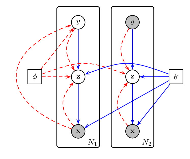
As in a standard VAE (Kingma & Welling, 2014), the learning happens by optimizing a stochastic estimate of the (standard) evidence lower bound. The bound under the model with observed labels becomes

$$\mathcal{L}=\mathbb{E}_{\left.q_{\phi}\!\left({\mathbf{z}}\right|{\mathbf{x},y}\right)}[\log\left.p_{\theta}\!\left({\mathbf{x}}\right|{\mathbf{z}}\right)]-\operatorname{{D}_{KL}}[\left.q_{\phi}\!\left({\mathbf{z}}\right|{\mathbf{x},y}\right)||\left.p_{\theta}\!\left({\mathbf{z}}\right|{y}\right)],$$ (1)

where $\operatorname{{D}_{KL}}$ denotes the KL-divergence, and under the model with unobserved labels, the evidence lower-bound becomes

$$\begin{split}\mathcal{U}&=\mathbb{E}_{\left.q_{\phi}\!\left({y}\right|{\mathbf{x}}\right)}[\mathbb{E}_{\left.q_{\phi}\!\left({\mathbf{z}}\right|{\mathbf{x},y}\right)}[\log\left.p_{\theta}\!\left({\mathbf{x}}\right|{\mathbf{z}}\right)]-\operatorname{{D}_{KL}}[\left.q_{\phi}\!\left({\mathbf{z}}\right|{\mathbf{x},y}\right)||\left.p_{\theta}\!\left({\mathbf{z}}\right|{y}\right)]]\\ &=\sum_{y}\left.q_{\phi}\!\left({y}\right|{\mathbf{x}}\right)\mathbb{E}_{\left.q_{\phi}\!\left({\mathbf{z}}\right|{\mathbf{x},y}\right)}[\log\left.p_{\theta}\!\left({\mathbf{x}}\right|{\mathbf{z}}\right)]+\mathcal{H}(q_{\phi}(y|\mathbf{x}))\\ &~{}~{}~{}-\sum_{y}\left.q_{\phi}\!\left({y}\right|{\mathbf{x}}\right)\operatorname{{D}_{KL}}[\left.q_{\phi}\!\left({\mathbf{z}}\right|{\mathbf{x},y}\right)||\left.p_{\theta}\!\left({\mathbf{z}}\right|{y}\right)].\end{split}$$ (2)

However, in our experiments we considered a different (and looser) lowerbound than $\mathcal{U}$, denoted by  $\mathcal{U}^{\ast}$, defined as  $\mathcal{U}$ without the entropy term $\mathcal{H}(q_{\phi}(y|\mathbf{x}))$.

Combining the above results in our semi-supervised objective: $\mathcal{S}=\mathcal{L}+\mathcal{U}^{\ast}$ , but in practice we also use an additional term, similar to the one used in Kingma et al. (2014), to train the classifier:

$$\mathcal{C}=\mathbb{E}_{p_{\text{emp.}}(\mathbf{x},y)}[\log(\left.q_{\phi}\!\left({y}\right|{\mathbf{x}}\right))],$$ (3)

where $p_{\text{emp.}}(\mathbf{x},y)$ denotes the empirical distribution over labeled data. We introduce this term, because in the original objective only the unlabeled objective is dependent on $\left.q_{\phi}\!\left({y}\right|{\mathbf{x}}\right)$. This additional term trains the classifier with the labeled samples used in the supervised lower bound calculation.

We add the additional term with a multiplier to the semi-supervised objective to get the full objective:

$$\mathcal{S}=\mathcal{L}+\mathcal{U}^{\ast}+\alpha\cdot\mathcal{C}$$ (4)

As usual with VAEs, we cannot compute the lower bounds exactly, but take Monte Carlo-estimates of them, and by the reparametrization trick (Kingma & Welling, 2014; Rezende et al., 2014), we are able to optimize the estimates so that the generation and inference networks parameters are tuned concurrently, i.e. in concerted fashion.

2.2 Nominal classification

In a nominal classification task, we try to predict a discrete class label $y^{(i)}\in\{0,1,...L-1\}$ for an observation $\mathbf{x}^{(i)}$. We can infer probabilities for each class label, given an example, using a nominal classifier. Usual choice for encoding the categorical distribution under a neural network is via the softmax:

$$\operatorname{softmax}(y_{k};\mathbf{x})=\frac{\exp{\{{\mathbf{W_{k}}}^{\top}\mathbf{h}{(\mathbf{x})}+b_{k}\}}}{\sum_{\ell}\exp{\{{\mathbf{W}_{\ell}}^{\top}\mathbf{h}{(\mathbf{x})}+b_{\ell}\}}},$$ (5)

where $\mathbf{W_{k}}$ and $b_{k}$ denote the class specific mapping vector and bias and the $\mathbf{h(\mathbf{x})}$ denote a neural network mapping of $\mathbf{x}$. We chose softmax to encode the categorical distribution of $q_{\phi}(y|\mathbf{x})$. The classification of an example $\mathbf{x}^{(i)}$ is then by evaluating the probabilibities with it, and the class is set to the label which gives the highest probability under it, i.e.

$$y^{(i)}_{\ast}=\operatorname*{argmax}_{k}q_{\phi}(y^{(i)}=k|\mathbf{x}^{(i)}).$$

2.3 Ordinal classification

Ordinal classification, also called ordinal regression, is a classification task where the discrete class labels have an order amongst them. In such setting, the classification loss is not only a function of the misclassification, but also the distance from the misclassified label to the correct one (Gutiérrez et al., 2016). Example of such a case could be diagnosis of a disease, where classifying the grade of disease lower than the actual grade, would cause progressively higher risk of fatality, the further the predicted grade is from the correct one. On the other hand, classifying the grade higher than the actual grade would cause progressively higher costs resulting from unnecessary treatment. (Pedregosa et al., 2017)

Multiple different techniques exist in the domain of ordinal classification. Using nominal classification methods is a simple approach and often ignores any ordinal features present in the data. For example, standard softmax classifier tries to partition the features in input data to orthogonal directions. Only the features in the direction of a class-dependent softmax weight vector will cause a response. This method clearly fails in a situation where the features are all in the same direction, but the magnitude separates different classes.

Choices for ordinal classifiers include (but is not restricted to): standard regression with prediction determined by nearest label to the output (Pedregosa et al., 2017) (Gutiérrez et al., 2016), using the expected value of nominal classifier prediction and minimizing the squared distance to the target (Beckham & Pal, 2016), cumulative link models that use scalar mappings to estimate cumulative probabilities for class labels, such as $\left.p\!\left({y\preceq\mathbf{y_{k}}}\right|{\mathbf{x}}\right)=f(\mu_{k}-W^{T}x)$ (Gutiérrez et al., 2016), Gaussian Processes (GP) (Chu & Ghahramani, 2005) and Support Vector Machines (SVM) (Herbrich et al., 1999).

What many ordinal methods have in common is the use of a scalar output function and a set of thresholds, which function as decision boundaries. A set of such thresholds could be, using similar notation as in  Gutiérrez et al. (2016), $\mathbf{b}=(b_{1},b_{2},...,b_{L-1})$. This set of thresholds defines intervals, usually with the beginning point of first interval set to negative infinity and the end of last interval to infinity. Every interval is associated to predicting a certain class. Using a function with a scalar output, we would predict class $i$ if $f(\mathbf{x})\in[b_{i-1},b_{i}]$.

For the purpose of enabling marginalization in ordinal domain, we developed an ordinal version of softmax with connection to the forementioned threshold methods. The form of this classifier is as follows:

$$\operatorname{ordmax}(y=k;\mathbf{x})=\frac{\exp{\{-({\mathbf{W}}^{\top}\mathbf{h(\mathbf{x})}+b-\mu_{k})^{2}/s\}}}{\sum_{\ell}\exp{\{-({\mathbf{W}}^{\top}\mathbf{h(\mathbf{x})}+b-\mu_{\ell})^{2}/s\}}},$$ (6)

where $\mu_{k}<\mu_{k+1}~{}\forall~{}k\in[1,2,\ldots,K-1]$. Similarly as softmax, the partition term is the sum of all the individual terms in this classifier, and the assigned probability to one class label is the weight the corresponding term has in the sum. This ensures that the probabilities sum up to one. The magnitudes of individual terms are defined by the learnable mapping ${\mathbf{W}}^{\top}\mathbf{h(\mathbf{x})}+b$ which outputs a scalar. The ordinality is introduced to the model, by defining the distribution centres $\mu_{k}$ as constant scalars with magnitudes increasing with the index. Thus the resulting probabilities have a peak on the class with closest centre to the mapping and the other probabilities decrease progressively the further we get away from this closest class. In our experiments, each the $\mu$’s was set to the numerical value of the corresponding label, shifted so that the mean value of $\mu$’s was zero.

We also introduced the learnable scaling factor $s$ to help in stabilization of the learning process. The point of $s$ is to flatten the initial distribution such that the initial probabilities would be more evenly distributed. As the model becomes more confident in its predictions it can decrease $s$ to concentrate more probability into its predictions. Without $s$ and centering the $\mu$’s, we ran into numerical issues in calculating cross-entropy, as often the log term was rounded into negative infinity.

2.4 Related work

The natural comparison of this model is with the generative semi-supervised model M2 described in Kingma et al. (2014). Their M2 model considers the generative process to be a function of statistically independent $y$ and $\mathbf{z}$ such that $p_{\theta}(y,\mathbf{z})=p_{\theta}(y)p_{\theta}(\mathbf{z})$, with $p_{\theta}(y)$ categorical – and $p_{\theta}(\mathbf{z})$ standard normal distribution. In our model the latent variables and the class information are not independent, but $\mathbf{z}$ has a conditional normal distribution given $y$. In the M2 model the prior $p_{\theta}(\mathbf{z})$ is a spherical Gaussian, with no learnable parameters, whereas our model $\left.p_{\theta}\!\left({\mathbf{z}}\right|{y}\right)$ consists of learnable mean vectors and diagonal covariance matrices.

The computational complexity of M2 model, described in Kingma et al. (2014) section 3.3, is stated to be that of $LC_{M1}$, where $C_{M1}$ is the computational complexity of their other model M1 and $L$ is the number of classes. The $C_{M1}$ includes the computational costs of both recognition and generative networks. In contrast to M2 model, our model would have the computational complexity (assuming same network configuration as in their M2 experiments and that summation is negligible compared to neural computations) $\frac{C_{M1}}{2}(L+1)$, as our model requires only one pass over recognition network and the marginalisation is performed by $L$ sums and passes over the generative network.

One another variational autoencoder approach that enables semi-supervised learning is described in Maaløe et al. (2016), but in addition to the approaches in Kingma et al. (2014) it has not been applied to ordinal classification. Also in contrast to our approach, it defines stochastically deep models, which we have excluded from the scope of this paper.

A similar appearance to our lower bound formulation appears in Sohn et al. (2015), but in contrast to their CVAE model, ours has no recognition network parameters for the latent prior distribution, which is defined by class conditional parameters and ours has no generative network parameters for the class label $y$. Judging from their lower bound formulation (equation (4)) and their graphical visualisation of conditional dependence (Figure 1), our lower bound is different from theirs.

There has been some previous work on semi-supervised ordinal regression. Supervised Gaussian processes for ordinal regression were used in Chu & Ghahramani (2005), and a semi-supervised version was introduced in Srijith et al. (2013). Also variational Gaussian process auto-encoders were developed in Eleftheriadis et al. (2016) for ordinal prediction of facial action units. Other techniques include kernel discriminant analysis with an additional order forcing term (Pérez-Ortiz et al., 2016).

3 Experiments and Results

In this section we will present some of our results using benchmark datasets on both nominal - and ordinal classification. We will also present some visualizations to better explain the inner workings of the model. We used the Python-based Theano-framework in our algorithm implementations (Theano Development Team, 2016).

3.1 Modelling and classifying MNIST-digit data

The MNIST dataset consists of 28 x 28 grayscale images of handwritten digits. We obtained the dataset directly from Yann LeCun’s website (LeCun et al., ) and divided the given training set onto a training and a validation set of size 50 000 and 10 000, respectively. We also used the data preprocessing scheme detailed in the Kingma et al. (2014). This preprocessing included data normalization to interval [0,1] and sampling individual pixels from a Bernoulli distribution using these normalized pixel intensities as success probabilities.

3.1.1 Generative modelling

We experimented on generative modelling with multiple different settings of hidden layers, hidden neurons, latent neurons and fractions of labelled data. Common settings for all our trained models were the use of softplus non-linearity and sigmoid function in the generative model output. Sigmoid function was used, because generative model distribution was chosen to be Bernoulli. This way the output neurons can be always interpreted as individual Bernoulli success probabilities and standard cross-entropy used in the objective function. In optimization, we used the Adam algorithm described in Kingma & Ba (2015).

Figure 2: Sampling from an MNIST-model: Images of the sampling distribution $\left.p_{\theta}\!\left({\mathbf{x}}\right|{\dot{\mathbf{z}}}\right)$ mean, given 25 random samples $\dot{\mathbf{z}}$ from $\left.p_{\theta}\!\left({\mathbf{z}}\right|{y}\right)$, the distribution of the latent variables conditional on the class label $y$, under each of the 10 classes.

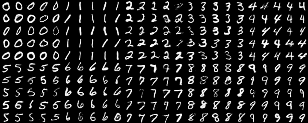
We observed that the visual quality of the samples was enhanced with adding layers to the model and also by increasing the amount of labelled data available to the model. The resulting digits, shown in Figure 2, represent samples from the learned latent prior distributions of a model with two hidden layers on all networks and 10000 labelled samples available to the model.

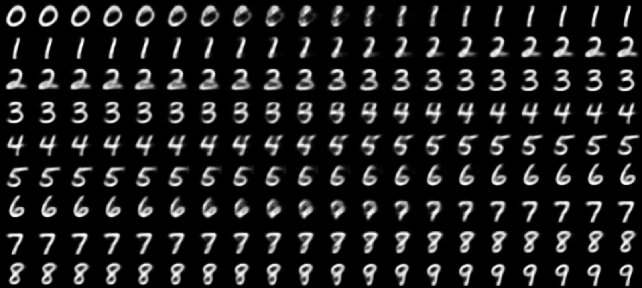
We observed that even thought removing layers and the amount of labelled data degraded the visual quality of the samples produced by the model, the reconstructions of interpolations between the latent distribution centres were well defined. We can see from Figure 3, how the linear interpolations in 50 dimensional latent space result in transformations from the original digit (shown in the left) towards the target digit (shown in the right). This model had one hidden layer on all networks with 500 hidden neurons and 1000 labelled examples available. The effect of latent space interpolation has been also considered in Nash & Williams (2017, see Fig. 11) but under different semantics.

Figure 3: Class-interpolated sampling from an MNIST-model: Images of the sampling distribution $\left.p_{\theta}\!\left({\mathbf{x}}\right|{\mathbf{z}}\right)$ mean under multiple configurations of (50-dimensional) $\mathbf{z}$, with one configuration per image. The configurations per each row start (first column) from the mean of $\left.p\!\left({\mathbf{z}}\right|{y=k}\right)$ (the probability distribution of the latent variables configuration conditional on the class label $y$ being $k$), and linearly interpolate to (last column) the mean of $\left.p_{\theta}\!\left({\mathbf{z}}\right|{y=k+1}\right)$ (the probability distribution of the latent variables configuration conditional on the class label $y$ being $k+1$). We can see that the interpolation results in semantically smooth digit morphs.

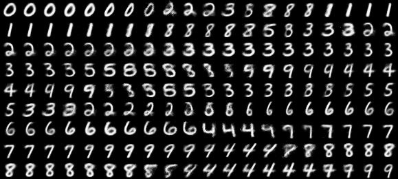
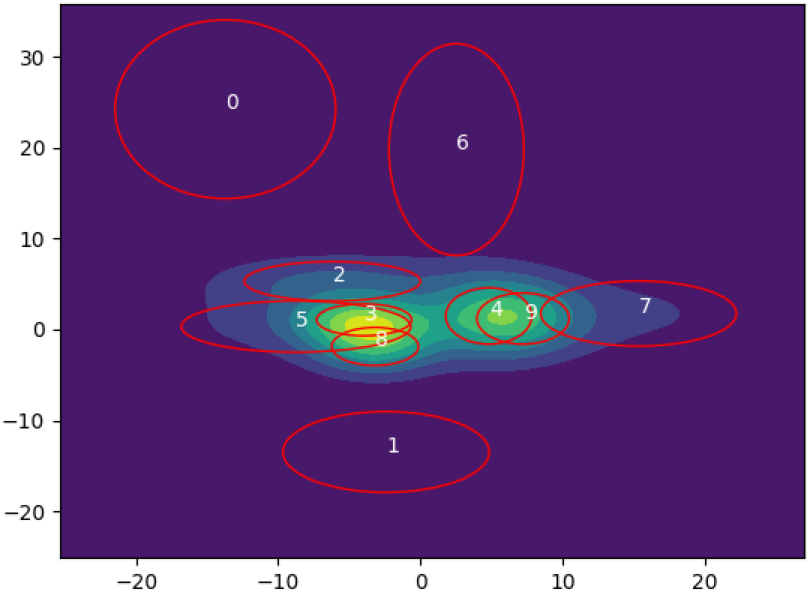
Decreasing the dimensionality of $\mathbf{z}$ to 2 allows us to visualize the distributions in the latent space. We observed that in this case, keeping the last network configuration resulted in poor performance, but by compensating the loss of latent dimensionality by adding one additional hidden layer, more hidden neurons and increasing the number of labelled samples increased the model performance to comparable results with the previous model. However the number of labelled examples had to be increased up to 40000. We can see from Figure 5 that digits with similar features seem to get close to one another. Interpolation between consecutive digits in this lower dimensional space shows how the latent distributions get more interleaved, as different digits appear on the way from one digit to another in Figure 4.

Figure 4: Class-interpolated sampling from model with 2-dimensional latent space. Visual inspection of Figure 4 explains the different digits appearing in the interpolation, as we pass through other distributions in latent space.

Figure 5: Class-conditional 2D-latent variable prior-distributions, and their mixture. Each (red) ellipse marks equiprobable points under a conditional distribution, with distribution mean at the center (and respective class label nearby), and points on the minor and major axis a standard deviation away from it. The background colouring encodes the mixture density.

3.1.2 Nominal classification

In semi-supervised classification task, we chose our network complexity to match that of M2 in Kingma et al. (2014). This means one hidden layer in both recognition and generative networks, both with 500 neurons. The latent $\mathbf{z}$ consists of 50 neurons and the classifier network is also one hidden layer with 500 neurons and a softmax classifier. As in generative modelling, the activations were chosen as softplus activations aside from the sigmoid activation on the generative network output, both similar choices to  Kingma et al. (2014). We chose to only compare our model to the M2 as both have similar stochastic depth, only one layer of stochastic variables, and by the same configuration they also have similar number of learned parameters.

The results of classification errors on different number of labelled data can be seen in Table 1. We can see that our model achieves lower error rates on average in the cases of 100, 600 and 3000 labelled examples, however ours has higher standard deviation on the cases 100 and 600. We can also see that there is consistency in our model performance, as the error always decreases on average by adding more labelled data to the supervised set.

Table 1: Semi-supervised MNIST classification statistics: Error using different amounts of labelled examples with the training set, comparing the proposed approach and results of the M2-model in Kingma et al. (2014, reproduced from Table 1). MEAN denotes the mean (lowest highlighted), and STD the standard deviation, of classification error. We have used 10 different runs (each choosing labeled examples randomly) to compute our results.

	Result statistics		Amount labeled
VAE	MEAN	STD
			100
M2	11.97	1.71
Us	8.16	3.22
			600
M2	4.94	0.13
Us	4.62	0.23
			1000
M2	3.60	0.56
Us	4.32	0.22
			3000
M2	3.92	0.63
Us	3.85	0.25

3.2 Modelling and classifying Stocks-data

We tested the flexibility of our model by implementing it to semi-supervised ordinal regression. We used the ordinal regression benchmark dataset ’stock domain’ (Chu, 2004). This dataset consists of 950 samples, with 9 features and an ordinal label. According to the authors Chu & Ghahramani (2005), this dataset was created from a standard regression problem, by binning the target regression interval into 5 equal length bins each representing one label. We divided these 950 samples 10 times into partitions of 600 training samples and 350 test samples. We used these partitions to train and evaluate model performance with multiple different fractions of labeled training data. In our experiments normalizing the data to zero-mean and unit variance proved to have a stabilizing effect on the learning process.

3.2.1 Generative modelling

The features of this dataset are all continuous values, thus the natural choice for the generative network output distribution is Gaussian. We also used a data-independent global variance for the Gaussian distribution, instead of a neural network mapping from the latent variables. This variance parameter was also learned by the model. Since there are only 9 features in the data, we used considerably smaller network than what we used in the MNIST experiments. The network had 1 hidden layer on both recognition – and generative model and both had 7 neurons. We used only one neuron for the latent feature layer and for the non-linearity, we chose hyperbolic tangent (tanh) activation.

3.2.2 Ordinal classification

The fractions of labeled data was set to similar values as used in Srijith et al. (2013). The fractions represent the ratio of labeled – to all training data. These fractions were created by sampling a subset of training data for which we kept the labels and discarded them for the rest. For comparison we also trained the model on the ordinal data using standard softmax with the rest of the model kept the same. Both classifiers also had a one hidden layer MLP connection from the data with hyperbolic tangent nonlinearity.

Table 2: Stock domain-dataset classification statistics: Error using different fractions of labelled to all data, comparing the two approaches. MEAN denotes the mean (lowest highlighted), and STD the standard deviation, of classification (zero-one) error.

	Result statistics		Fraction (labeled)
Softmax	MEAN	STD
			0.05
Standard	0.354	0.069
Ordinal	0.333	0.063
			0.10
Standard	0.283	0.044
Ordinal	0.258	0.038
			0.15
Standard	0.258	0.041
Ordinal	0.219	0.037
			0.20
Standard	0.224	0.041
Ordinal	0.206	0.030
			0.25
Standard	0.217	0.029
Ordinal	0.198	0.026
			0.30
Standard	0.203	0.025
Ordinal	0.189	0.017

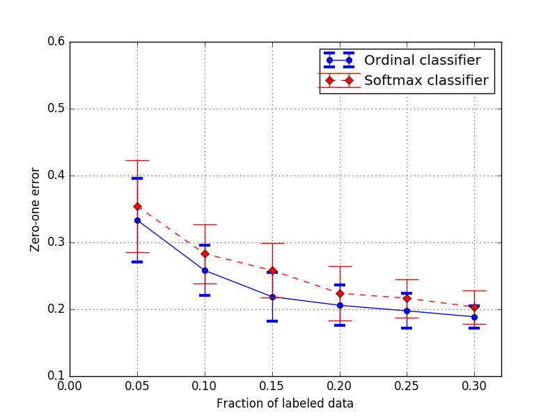
We present the test set errors for both models in Table 2. We can see that in all cases the ordinal classifier had better accuracy than the softmax classifier using the same amount of labeled data. However, in most cases the difference is within the margin of one standard error. Reader is also recommended to compare our results shown in Figure 6 to the ones provided in Srijith et al. (2013) - Figure 2. By visual inspection, we can see similar performance in our model.

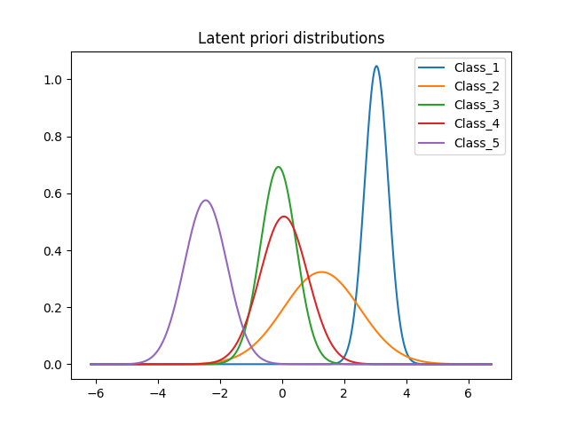
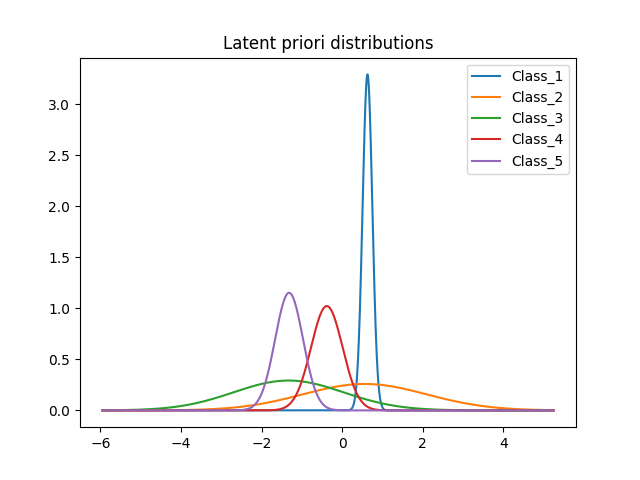
In the Fig. 7 and 8 we can see examples of the one dimensional learned priori distributions for this ordinal data. For the ordinal classifier case there seems to be high mixing of the classes 3 and 4. In the softmax classifier case, we see that classes 2 and 3 have very flat distributions and the peaks seem to match the peaks of classes 1 and 5. Class one has very concentrated mass which results in a peak in the figure.

Figure 6: Stock domain-classification statistics: Classifier accuracy using different fractions of labelled to all data, comparing the two approaches.

Figure 7: One dimensional latent space, Ordinal classifier: Ordering of the latent space using ordinal classifier.

Figure 8: One dimensional latent space, Softmax classifier: Ordering of the latent space using softmax classifier.

4 Summary and Discussion

We have introduced a novel variational autoencoder, which we have shown to be capable of learning features from both nominal - and ordinal data in semi-supervised manner, with results comparable to similar complexity models specifically designed for these types of data. Our model also enables easy interpretation of the learned class-wise features, as each class has their own distinct distributions.

Our main future work is on retinal image analysis, including semi-supervised retinal image classification, for which we have developed a convolutional variant of our model. Because the label information is introduced as a bias to the latent mean parameter, the fully-connected networks can be replaced with convolutional ones and the model parametrisation is still intuitive. One interesting avenue of further research could include a deep stochastic variant of our model, with multiple layers of stochastic variables $\mathbf{z}$. This would also make the model more comparable to the forementioned deep stochastic models. Such extensions could be useful in an another interesting avenue of further research, developing extensions for semi-supervised retinal image (semantic) segmentation.

As we saw, e.g. with the 2D latent space illustration of Fig. 5, in low dimensions the latent distributions may get significantly interleaved. One avenue of future research is to introduce an objective that would separate these distributions in a controlled manner during the training process. One such objective could be by the multi-class version of the Fisher’s linear discriminant applied to the latent prior distributions to encourage their separation. This way it could be possible to get good class separation, using lower number of latent neurons.

References

- Beckham & Pal (2016) Beckham, C. and Pal, C. A simple squared-error reformulation for ordinal classification. In Extended abstract, Advances in Neural Information Processing (NIPS), Workshop on Machine Learning for Health, 2016. arXiv:1612.00775v2 [stat.ML].
- Burda et al. (2016) Burda, Y., Grosse, R., and Salakhutdinov, R. Importance weighted autoencoders. In Proc., International Conference on Learning Representations (ICLR), 2016. arXiv:1509.00519v4 [cs.LG].
- Chu (2004) Chu, W. BENCHMARK of ORDINAL REGRESSION: datasets and results, 2004. URL: http://www.gatsby.ucl.ac.uk/~chuwei/ordinalregression.html [version 2004.08.11, cited 11 Oct. 2017].
- Chu & Ghahramani (2005) Chu, W. and Ghahramani, Z. Gaussian processes for ordinal regression. Journal of Machine Learning Research (JMLR), 18, 2005.
- Dayan et al. (1995) Dayan, P., Hinton, G. E., Neal, R. M., and Zemel, R. S. The Helmholtz machine. Neural Comp., 7, 1995.
- Eleftheriadis et al. (2016) Eleftheriadis, S., Rudovic, O., Deisenroth, M. P., and Pantic, M. Variational Gaussian process auto-encoder for ordinal prediction of facial action units, 2016. arXiv:1608.04664v2 [stat.ML].
- Gutiérrez et al. (2016) Gutiérrez, P. A., Pérez-Ortiz, M., Sánchez-Monedero, J., Fernández-Navarro, F., and Hervás-Martínez, C. Ordinal regression methods: Survey and experimental study. IEEE Trans. KDE, 28, 2016.
- Herbrich et al. (1999) Herbrich, R., Graepel, T., and Obermayer, K. Support vector learning for ordinal regression. In Proc., International Conference on Artificial Neural Networks (ICANN), 1999.
- Hinton et al. (1995) Hinton, G. E., Dayan, P., Frey, B., and Neal, R. M. The ”wake-sleep” algorithm for unsupervised neural networks. Science, 268, 1995.
- Kingma & Ba (2015) Kingma, D. P. and Ba, J. Adam: A method for stochastic optimization. In Proc., International Conference on Learning Representations (ICLR), 2015. arXiv:1412.6980v9 [cs.LG].
- Kingma & Welling (2014) Kingma, D. P. and Welling, M. Auto-encoding variational bayes. In Proc., International Conference on Learning Representations (ICLR), 2014. arXiv:1312.6114v10 [stat.ML].
- Kingma et al. (2014) Kingma, D. P., Mohamed, S., Rezende, D. J., and Welling, M. Semi-supervised learning with deep generative models. In Proc., Advances in Neural Information Processing Systems (NIPS), 2014.
- (13) LeCun, Y., Cortes, C., and Burges, C. J.C. THE MNIST DATABASE of handwritten digits. URL: http://yann.lecun.com/exdb/mnist/ [cited 11 Oct. 2017].
- Maaløe et al. (2016) Maaløe, L., Sønderby, C. K., Sønderby, S. K., and Winther, O. Auxiliary deep generative models. In Proc., International Conference on Machine Learning (ICML), 2016. arXiv:1602.05473v4 [stat.ML].
- MacKay & Gibbs (1998) MacKay, D. J. C. and Gibbs, M. N. Density networks. Statistics and Neural Networks, 1998.
- Nash & Williams (2017) Nash, C. and Williams, C. K. I. The shape variational autoencoder: A deep generative model of part-segmented 3D objects. Computer Graphics Forum, 36(5), 2017. ISSN 1467-8659. doi: 10.1111/cgf.13240.
- Pedregosa et al. (2017) Pedregosa, F., Bach, F., and Gramfort, A. On the consistency of ordinal regression methods. Journal of Machine Learning Research (JMLR), 18, 2017.
- Pérez-Ortiz et al. (2016) Pérez-Ortiz, M., Gutiérrez, P. A., Carbonero-Ruz, M., and Hervés-Martínez, C. Semi-supervised learning for ordinal kernel discriminant analysis. Neural Networks, 84, 2016.
- Rezende et al. (2014) Rezende, D. J., Mohamed, S., and Wierstra, D. Stochastic backpropagation and approximate inference in deep generative models. In Proc., International Conference on Machine Learning (ICML), 2014. arXiv:1401.4082[stat.ML].
- Sohn et al. (2015) Sohn, K., Lee, H., and Yan, X. Learning structured output representation using deep conditional generative models. In Proc., Advances in Neural Information Processing Systems (NIPS), 2015.
- Sønderby et al. (2016) Sønderby, C. K., Raiko, T., Maaløe, L., Sønderby, S. K., and Winther, O. Ladder variational autoencoders. In Proc., Advances in Neural Information Processing Systems (NIPS), 2016.
- Srijith et al. (2013) Srijith, P. K., Shevade, S., and Sundararajan, S. Semi-supervised Gaussian process ordinal regression. In Proc., European Conference on Machine Learning and Principles and Practice of Knowledge Discovery in Databases (ECML-PKDD), 2013.
- Theano Development Team (2016) Theano Development Team. Theano: A Python framework for fast computation of mathematical expressions. arXiv e-prints, abs/1605.02688, May 2016. URL: http://arxiv.org/abs/1605.02688.