Analysis of the $(\mu/\mu_{I},\lambda)$-$\sigma$-Self-Adaptation Evolution Strategy with Repair by Projection Applied to a Conically Constrained Problem

Abstract

A theoretical performance analysis of the $(\mu/\mu_{I},\lambda)$-$\sigma$-Self-Adaptation Evolution Strategy ($\sigma$SA-ES) is presented considering a conically constrained problem. Infeasible offspring are repaired using projection onto the boundary of the feasibility region. Closed-form approximations are used for the one-generation progress of the evolution strategy. Approximate deterministic evolution equations are formulated for analyzing the strategy’s dynamics. By iterating the evolution equations with the approximate one-generation expressions, the evolution strategy’s dynamics can be predicted. The derived theoretical results are compared to experiments for assessing the approximation quality. It is shown that in the steady state the $(\mu/\mu_{I},\lambda)$-$\sigma$SA-ES exhibits a performance as if the ES were optimizing a sphere model. Unlike the non-recombinative $(1,\lambda)$-ES, the parental steady state behavior does not evolve on the cone boundary but stays away from the boundary to a certain extent.

I Introduction

Current research in evolution strategies includes the design and analysis of evolution strategies applied to constrained optimization problems. It is of particular interest to gain a deep understanding of evolution strategies on such problems. The insights gained from theory can help to provide guidance in applying evolution strategies to real world constrained problems. First, theory can show what kind of problems are suitably solved by evolution strategies. Moreover, theoretical investigations can guide the design of ES algorithms. And furthermore, theoretically derived suggestions for (optimal) parameter settings can be provided.

Arnold has analyzed a $(1,\lambda)$-ES with constraint handling by resampling for a single linear constraint [1]. This has been extended in [2] with the analysis of repair by projection for a single linear constraint. This repair approach has been compared with an approach that reflects infeasible points into the feasible region and an approach that truncates infeasible points in [3]. Another idea for constraint handling based on augmented Lagrangian constraint handling has been presented in [4] for a $(1+1)$-ES. There, a single linear inequality constraint with the sphere model is considered. For this, the one-generation behavior was analyzed.

A multi-recombinative variant of this algorithm has been presented in [5] for a single linear constraint and multiple linear constraints in [6]. Markov chains have been used in both cases for a theoretical investigation.

A conically constrained problem is considered in [7]. There, a $(1,\lambda)$-ES is applied to the problem using death penalty, i.e., infeasible offspring are discarded until feasible ones are obtained. Theoretical investigations have been performed for this constellation. The same problem has been investigated in [8]. There, a $(1,\lambda)$-$\sigma$-Self-Adaptation ES has been applied. Repair by projection instead of discarding infeasible offspring has been used. This paper extends that work to the multi-recombinative variant, the $(\mu/\mu_{I},\lambda)$-$\sigma$-Self-Adaptation ES.

The rest of the paper is organized as follows. The optimization problem is described in Section II. This is followed by a presentation of the algorithm under consideration in Section III. Next, the theoretical results are presented. First, the dynamical systems analysis approach is briefly recapped in Section IV-A. Then, the algorithm’s behavior from one generation to the next (microscopic behavior) is investigated in Section IV-B. This is followed by the multi-generation behavior (macroscopic behavior) in Section IV-C. Closed-form approximations under asymptotic assumptions are derived for the microscopic behavior. They are then used in deterministic evolution equations. These evolution equations are iterated in order to predict the mean value dynamics of the ES. The approximations are compared to simulations. Finally, the insights gained are discussed in Section V. In particular, the differences and similarities of the $(1,\lambda)$-ES and the multi-recombinative variant are discussed.

II Optimization Problem

The optimization problem under consideration is

$$f(\mathbf{x})=x_{1}\rightarrow\text{min}!$$ (1)

subject to constraints

$$x_{1}^{2}-\xi\sum_{k=2}^{N}x_{k}^{2} \geq 0$$ (2)

$$x_{1} \geq 0$$ (3)

where $\mathbf{x}=(x_{1},\ldots,x_{N})^{T}\in\mathbb{R}^{N}$ and $\xi>0$.

The distance $x$ from $0$ in $x_{1}$-direction (cone axis) and the distance $r$ from the cone’s axis suffices to describe the state of the ES in the search space. This is denoted as the $(x,r)^{T}$-space in the following. Moreover, note that due to the isotropy of the mutations used in the ES, the coordinate system can w.l.o.g. be rotated. Thus, an objective parameter vector’s distance from the cone axis coincides with the second component of this rotated coordinate system, i.e., $(\tilde{x},\tilde{r})^{T}$ corresponds to $(\tilde{x},\tilde{r},0,\ldots,0)^{T}$, see Fig. 1. The cone boundary is described by the equation $r=\frac{x_{1}}{\sqrt{\xi}}$, which follows from Equation 2. One arrives at the equation of the projection line by the cone direction $\left(1,\frac{1}{\sqrt{\xi}}\right)^{T}$ and $\left(-\frac{1}{\sqrt{\xi}},1\right)^{T}$ (counterclockwise rotation by 90 degrees). With this, $r=-\sqrt{\xi}x_{1}+q\left(\sqrt{\xi}+\frac{1}{\sqrt{\xi}}\right)$ follows as the equation for the projection line. A parent $\mathbf{x}$ and an offspring $\tilde{\mathbf{x}}$ with the mutation $\tilde{\sigma}\mathbf{z}$ are visualized as well. The values $q$ and $q_{r}$ denote the $x_{1}$ and $r$ values after the projection step.

Figure 1: The conically constrained optimization problem in $N$ dimensions shown in the $(x,r)^{T}$-space.

III Algorithm

A $(\mu/\mu_{I},\lambda)$-$\sigma$-Self-Adaptation ES is applied to the optimization problem described in Section II. Algorithm 1 shows the pseudo code. First, parameters are initialized (1 to 2). After that, the generation loop is entered. $\lambda$ offspring are generated in 6 to 15. A log-normal distribution is used for every offspring to compute its mutation strength $\tilde{\sigma}_{l}$ by mutating the parental mutation strength $\sigma^{(g)}$ (7). Using this determined mutation strength, the offspring’s parameter vector is sampled from a multivariate normal distribution with mean $\mathbf{x}^{(g)}$ and standard deviation $\tilde{\sigma}_{l}$ (8). Then, the offspring is repaired by projection, if necessary (9 to 11). This means that for infeasible offspring, the optimization problem

$$\begin{split}\mathbf{\hat{x}}=\operatorname*{arg\,min}_{\mathbf{x^{\prime}}}\lVert\mathbf{x^{\prime}}-\mathbf{x}\rVert^{2}\\ \text{s.t. }{x^{\prime}_{1}}^{2}-\xi\sum_{k=2}^{N}{x^{\prime}_{k}}^{2}\geq 0\\ x^{\prime}_{1}\geq 0\end{split}$$ (4)

must be solved where $\mathbf{x}$ is the individual to be projected. For this, a helper function

$$\mathbf{\hat{x}}=\text{projectOntoCone}(\mathbf{x})$$ (5)

is introduced that returns $\hat{\mathbf{x}}$ of (4). A derivation for a closed-form solution to this projection optimization problem (4) is presented in the supplementary material in Appendix A. $x^{(g)}$, $r^{(g)}$, $q_{l}$, $\mathbf{q^{\prime}}_{l}$, $\langle q\rangle$, and $\langle q_{r}\rangle$ (4, 5, 13, 14, 19, and 20) are values used in the theoretical analysis. They can be removed in practical implementations of the ES. The offspring’s fitness is computed in 12. The next generation’s parental individual $\mathbf{x}^{(g+1)}$ (17) and the next generation’s mutation strength $\sigma^{(g+1)}$ (18) are updated next. The parental parameter vector for the next generation is set to the mean of the parameter vectors of the $\mu$ best offspring. Similarly, the parental mutation strength for the next generation is set to the mean of the mutation strengths of the $\mu$ best offspring. If the parental parameter vector for the next generation is not feasible, it is projected onto the cone (21 to 23). Note that this repair step is not needed in the real implementation of the algorithm. Since the conical problem is convex, the intermediate recombination of the $\mu$ best feasible individuals is feasible as well. However, in the iteration of the evolution equations in Section IV-C, the $(x,r)^{T}$ can get infeasible due to the approximations used. Finally, the generation counter is updated, which completes one iteration of the generational loop.

Algorithm 1 Pseudo-code of the $(\mu/\mu_{I},\lambda)$-$\sigma$-Self-Adaptation ES with repair by projection applied to the conically constrained problem.

1:Initialize $\mathbf{x}^{(0)}$, $\sigma^{(0)}$, $\tau$, $\lambda$, $\mu$

2:$g\leftarrow 0$

3:repeat

4:     $x^{(g)}=(\mathbf{x}^{(g)})_{1}$

5:     $r^{(g)}=\sqrt{\sum_{k=2}^{N}(\mathbf{x}^{(g)})_{k}^{2}}$

6:     for $l\leftarrow 1\textbf{ to }\lambda$ do

7:         $\tilde{\sigma}_{l}\leftarrow\sigma^{(g)}e^{\tau\mathcal{N}(0,1)}$

8:         $\tilde{\mathbf{x}}_{l}\leftarrow\mathbf{x}^{(g)}+\tilde{\sigma}_{l}\mathcal{N}(\mathbf{0},\mathbf{I})$

9:         if not isFeasible($\tilde{\mathbf{x}}_{l}$) then $\triangleright$ see Algorithm 2

10:              $\tilde{\mathbf{x}}_{l}\leftarrow$ projectOntoCone($\tilde{\mathbf{x}}_{l}$) $\triangleright$ see (4), (5)

11:         end if

12:         $\tilde{f}_{l}\leftarrow f(\tilde{\mathbf{x}}_{l})=(\tilde{\mathbf{x}}_{l})_{1}$

13:         $q_{l}=(\tilde{\mathbf{x}}_{l})_{1}$

14:         $\mathbf{q^{\prime}}_{l}=\tilde{\mathbf{x}}_{l}$

15:     end for

16:     Sort offspring according to $\tilde{f}_{l}$ in ascending order

17:     $\mathbf{x}^{(g+1)}\leftarrow\frac{1}{\mu}\sum_{m=1}^{\mu}\tilde{\mathbf{x}}_{m;\lambda}$

18:     $\sigma^{(g+1)}\leftarrow\frac{1}{\mu}\sum_{m=1}^{\mu}\tilde{\sigma}_{m;\lambda}$

19:     $\langle q\rangle=(\mathbf{x}^{(g+1)})_{1}$

20:     $\langle q_{r}\rangle=\sqrt{\sum_{k=2}^{N}(\mathbf{x}^{(g+1)})_{k}^{2}}$

21:     if not isFeasible($\mathbf{x}^{(g+1)}$) then $\triangleright$ see Algorithm 2

22:         $\mathbf{x}^{(g+1)}\leftarrow$ projectOntoCone($\mathbf{x}^{(g+1)}$) $\triangleright$ see (4), (5)

23:     end if

24:     $g\leftarrow g+1$

25:until termination criteria are met

Algorithm 2 Feasibility check

1:function isFeasible($\mathbf{x}$)

2:     return($x_{1}\geq 0\land x_{1}^{2}-\xi\sum_{k=2}^{N}x_{k}^{2}\geq 0$)

3:end function

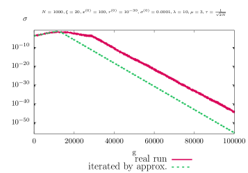
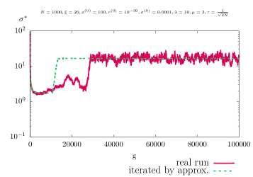
Fig. 2 shows an example of the $x$- and $r$-dynamics that are a result of running Algorithm 1 (solid line). The closed-form approximation iterative system (dotted line) (to be derived in the following sections) is shown in comparison. The prediction does not coincide completely with the real run. The ES reaches the stationary state later than predicted. The approximations that are derived in this work result in deviations in the transient phase of the ES. However, our main focus is in the steady state. There, the predicted slope of the $x$ and $r$ dynamics is very similar to the one of the real run.

Figure 2: Comparison of the $x$- and $r$-dynamics of a real $(3/3_{I},10)$-ES run (solid line) with the iteration of the closed-form approximation of the iterative system (dotted line).

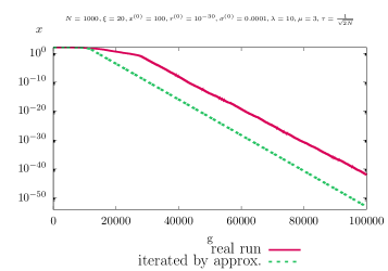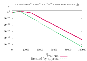IV Theoretical Analysis

IV-A The Dynamical Systems Approach

The $(x,r)^{T}$-representation described in Section II is used for the analysis of the $(\mu/\mu_{I},\lambda)$-ES (Algorithm 1). The aim is to predict the evolution dynamics of the $(\mu/\mu_{I},\lambda)$-ES. To this end, the dynamical systems method described in [9] is used. State variables of the strategy are modeled over time. For the case here, the three random variables for $x$, $r$, and $\sigma$ describe the state of the system. A Markov process can be used for modeling the transitions between states from one time step to the next. It is often not possible to derive closed-form expressions for the transition equations. Therefore, approximate equations are aimed for. Evolution equations can be stated by making use of the local expected change functions ($\varphi_{x},\varphi_{r},\psi$)

$$x^{(g+1)} =x^{(g)}-\varphi_{x}(x^{(g)},r^{(g)},\sigma^{(g)})+\epsilon_{x}(x^{(g)},r^{(g)},\sigma^{(g)})$$ (6)

$$r^{(g+1)} =r^{(g)}-\varphi_{r}(x^{(g)},r^{(g)},\sigma^{(g)})+\epsilon_{r}(x^{(g)},r^{(g)},\sigma^{(g)})$$ (7)

$$\sigma^{(g+1)} =\sigma^{(g)}+\sigma^{(g)}\psi(x^{(g)},r^{(g)},\sigma^{(g)})+\epsilon_{\sigma}(x^{(g)},r^{(g)},\sigma^{(g)}).$$ (8)

The progress rates are defined as

$$\varphi_{x}(x^{(g)},r^{(g)},\sigma^{(g)}):=\mathrm{E}[x^{(g)}-x^{(g+1)}\,|\,x^{(g)},r^{(g)},\sigma^{(g)}]$$ (9)

$$\varphi_{r}(x^{(g)},r^{(g)},\sigma^{(g)}):=\mathrm{E}[r^{(g)}-r^{(g+1)}\,|\,x^{(g)},r^{(g)},\sigma^{(g)}].$$ (10)

They model the expected change in the parameter space from one generation to the next. The random variables $\epsilon_{x}$, $\epsilon_{r}$, and $\epsilon_{\sigma}$ represent the stochastic part. $\mathrm{E}[\epsilon_{x}]=0$, $\mathrm{E}[\epsilon_{r}]=0$, and $\mathrm{E}[\epsilon_{\sigma}]=0$ necessarily holds.

In what follows, the normalizations

$$\varphi_{x}^{*}(\cdot):=\frac{N\varphi_{x}(\cdot)}{x^{(g)}},$$ (11)

$$\varphi_{r}^{*}(\cdot):=\frac{N\varphi_{r}(\cdot)}{r^{(g)}},$$ (12)

and

$$\sigma^{*}:=\frac{N\sigma}{r^{(g)}}$$ (13)

will be used. For the change of the mutation strength from one generation to the next, a slightly different progress measure will be applied. It is the so-called self-adaptation response (SAR). Its definition reads

$$\psi(x^{(g)},r^{(g)},\sigma^{(g)}):=\mathrm{E}\left[\frac{\sigma^{(g+1)}-\sigma^{(g)}}{\sigma^{(g)}}\,\bigg{|}\,x^{(g)},r^{(g)},\sigma^{(g)}\right].$$ (14)

$\epsilon_{x}=0$, $\epsilon_{r}=0$, and $\epsilon_{\sigma}=0$ is assumed in Equations 6 to 8 for the analysis in this work. That is, it is assumed that the fluctuations can be ignored for deriving approximate expressions for the evolution dynamics of the strategy for the case $N\rightarrow\infty$. Evolution equations without fluctuation terms are also known as deterministic evolution equations or mean value evolution equations. With the goal of arriving at approximate deterministic evolution equations, approximate expressions for the functions $\varphi_{x}$, $\varphi_{r}$, and $\psi$ need to be derived first.

IV-B The Microscopic Aspects

The microscopic aspects describe the behavior of the evolution strategy from one generation to the next. They are expressed by the functions introduced in Section IV-A (Equations 9, 10, and 14).

In the following analyses, two cases are treated separately. It turns out that if the parental individual is in the vicinity of the cone boundary, the offspring feasibility probability tends to $0$ for asymptotic considerations ($N\rightarrow\infty$). Hence, the local progress measures and the SAR are derived separately for the case of being at the cone boundary and for the opposite case. In order to have one approximate closed-form expression, they are combined by weighting with the feasibility probability. It is referred to [8, Sec. 3.1.2.1.2.8, pp. 44-49] for further details. There, the feasibility probability has been derived as

$$P_{\text{feas}}(x^{(g)},r^{(g)},\sigma^{(g)})\simeq\Phi\left[\frac{1}{\sigma^{(g)}}\left(\frac{x^{(g)}}{\sqrt{\xi}}-\bar{r}\right)\right]$$ (15)

where $\bar{r}$ is the expected value of the $r$ normal approximation and $\Phi$ is the cumulative distribution function of the standard normal variate. In order to simplify the theoretical analysis, the distribution of the $r$ component is approximated by a normal distribution. The supplementary material (Appendix B) presents a detailed derivation of this approximation.

IV-B1 Derivation of the $x$ Progress Rate

From the definition of the progress rate (Equation 9) and the pseudo-code of the ES (Algorithm 1, 19 and 4),

$$\varphi_{x}(x^{(g)},r^{(g)},\sigma^{(g)}) =x^{(g)}-\mathrm{E}[x^{(g+1)}\,|\,x^{(g)},r^{(g)},\sigma^{(g)}]$$ (16)

$$=x^{(g)}-\mathrm{E}[\langle q\rangle\,|\,x^{(g)},r^{(g)},\sigma^{(g)}]$$ (17)

follows. Therefore, $\mathrm{E}[\langle q\rangle\,|\,x^{(g)},r^{(g)},\sigma^{(g)}]:=\mathrm{E}[\langle q\rangle]$ needs to be derived to proceed further. Its derivation is presented in detail in the supplementary material in Appendix C.

Using the result from Equation C.169, the normalized $x$ progress rate for the feasible case can be formulated as

$${\varphi_{x}}_{\text{feas}}^{*} =\frac{N\left(x^{(g)}-\mathrm{E}[{\langle q\rangle}_{\text{feas}}]\right)}{x^{(g)}}$$ (18)

$$=\frac{N\left(x^{(g)}-x^{(g)}+\sigma^{(g)}c_{\mu/\mu,\lambda}\right)}{x^{(g)}}$$ (19)

$$=\frac{r^{(g)}}{x^{(g)}}{\sigma^{(g)}}^{*}c_{\mu/\mu,\lambda}.$$ (20)

In Equation 20, one of the so-called generalized progress coefficients $c_{\mu/\mu,\lambda}=e_{\mu,\lambda}^{1,0}$ defined in [9, Eq. (5.112), p. 172] appears. Their definition reads

$$\begin{multlined}e_{\mu,\lambda}^{\alpha,\beta}:=\frac{\lambda-\mu}{{(\sqrt{2\pi})}^{\alpha+1}}\binom{\lambda}{\mu}\\ \times\int_{t=-\infty}^{t=\infty}t^{\beta}e^{-\frac{\alpha+1}{2}t^{2}}[\Phi(t)]^{\lambda-\mu-1}[1-\Phi(t)]^{\mu-\alpha}\,\mathrm{d}t.\end{multlined}e_{\mu,\lambda}^{\alpha,\beta}:=\frac{\lambda-\mu}{{(\sqrt{2\pi})}^{\alpha+1}}\binom{\lambda}{\mu}\\ \times\int_{t=-\infty}^{t=\infty}t^{\beta}e^{-\frac{\alpha+1}{2}t^{2}}[\Phi(t)]^{\lambda-\mu-1}[1-\Phi(t)]^{\mu-\alpha}\,\mathrm{d}t.$$ (21)

Similarly, use of Equation C.224 results in

$$\begin{multlined}{\varphi_{x}}_{\text{infeas}}^{*}=\frac{N\left(x^{(g)}-\mathrm{E}[{\langle q\rangle}_{\text{infeas}}]\right)}{x^{(g)}}\end{multlined}{\varphi_{x}}_{\text{infeas}}^{*}=\frac{N\left(x^{(g)}-\mathrm{E}[{\langle q\rangle}_{\text{infeas}}]\right)}{x^{(g)}}$$ (23)

$$\begin{multlined}\phantom{{\varphi_{x}}_{\text{infeas}}^{*}}=\frac{N}{x^{(g)}}\left(\frac{1+\xi}{1+\xi}x^{(g)}-\mathrm{E}[{\langle q\rangle}_{\text{infeas}}]\right)\end{multlined}\phantom{{\varphi_{x}}_{\text{infeas}}^{*}}=\frac{N}{x^{(g)}}\left(\frac{1+\xi}{1+\xi}x^{(g)}-\mathrm{E}[{\langle q\rangle}_{\text{infeas}}]\right)$$ (25)

$$\begin{multlined}\phantom{{\varphi_{x}}_{\text{infeas}}^{*}}\approx\frac{N}{x^{(g)}}\left[\frac{x^{(g)}+\xi x^{(g)}-\xi x^{(g)}}{1+\xi}-\frac{\sqrt{\xi}\bar{r}}{1+\xi}\right.\\ \left.+\frac{\xi}{1+\xi}\left(\sqrt{{\sigma^{(g)}}^{2}+\sigma_{r}^{2}/\xi}\right)c_{\mu/\mu,\lambda}\right].\end{multlined}\phantom{{\varphi_{x}}_{\text{infeas}}^{*}}\approx\frac{N}{x^{(g)}}\left[\frac{x^{(g)}+\xi x^{(g)}-\xi x^{(g)}}{1+\xi}-\frac{\sqrt{\xi}\bar{r}}{1+\xi}\right.\\ \left.+\frac{\xi}{1+\xi}\left(\sqrt{{\sigma^{(g)}}^{2}+\sigma_{r}^{2}/\xi}\right)c_{\mu/\mu,\lambda}\right].$$ (28)

for the infeasible case. This can further be simplified using $\sigma_{r}$ of the normal approximation (Equation B.108) together with $\sigma$-normalization yielding

$$\begin{multlined}{\varphi_{x}}_{\text{infeas}}^{*}=\frac{N}{1+\xi}\biggl{[}1-\sqrt{\xi}\frac{r^{(g)}}{x^{(g)}}\sqrt{1+\frac{{{\sigma^{(g)}}^{*}}^{2}}{N}\left(1-\frac{1}{N}\right)}\\ +\xi\frac{r^{(g)}}{x^{(g)}}\sqrt{\frac{{{\sigma^{(g)}}^{*}}^{2}}{N^{2}}+\frac{1}{\xi}\frac{{{\sigma^{(g)}}^{*}}^{2}}{N^{2}}\frac{1+\frac{{{\sigma^{(g)}}^{*}}^{2}}{2N}(1-\frac{1}{N})}{1+\frac{{{\sigma^{(g)}}^{*}}^{2}}{N}(1-\frac{1}{N})}}c_{\mu/\mu,\lambda}\biggr{]}\end{multlined}{\varphi_{x}}_{\text{infeas}}^{*}=\frac{N}{1+\xi}\biggl{[}1-\sqrt{\xi}\frac{r^{(g)}}{x^{(g)}}\sqrt{1+\frac{{{\sigma^{(g)}}^{*}}^{2}}{N}\left(1-\frac{1}{N}\right)}\\ +\xi\frac{r^{(g)}}{x^{(g)}}\sqrt{\frac{{{\sigma^{(g)}}^{*}}^{2}}{N^{2}}+\frac{1}{\xi}\frac{{{\sigma^{(g)}}^{*}}^{2}}{N^{2}}\frac{1+\frac{{{\sigma^{(g)}}^{*}}^{2}}{2N}(1-\frac{1}{N})}{1+\frac{{{\sigma^{(g)}}^{*}}^{2}}{N}(1-\frac{1}{N})}}c_{\mu/\mu,\lambda}\biggr{]}$$ (31)

$$\begin{multlined}\phantom{{\varphi_{x}}_{\text{infeas}}^{*}}\simeq\frac{N}{1+\xi}\left[1-\sqrt{\xi}\frac{r^{(g)}}{x^{(g)}}\sqrt{1+\frac{{{\sigma^{(g)}}^{*}}^{2}}{N}}\right.\\ \left.\hskip 56.9055pt+\xi\frac{r^{(g)}}{x^{(g)}}\frac{{{\sigma^{(g)}}^{*}}}{N}\sqrt{1+\frac{1}{\xi}\frac{1+\frac{{{\sigma^{(g)}}^{*}}^{2}}{2N}}{1+\frac{{{\sigma^{(g)}}^{*}}^{2}}{N}}}c_{\mu/\mu,\lambda}\right].\end{multlined}\phantom{{\varphi_{x}}_{\text{infeas}}^{*}}\simeq\frac{N}{1+\xi}\left[1-\sqrt{\xi}\frac{r^{(g)}}{x^{(g)}}\sqrt{1+\frac{{{\sigma^{(g)}}^{*}}^{2}}{N}}\right.\\ \left.\hskip 56.9055pt+\xi\frac{r^{(g)}}{x^{(g)}}\frac{{{\sigma^{(g)}}^{*}}}{N}\sqrt{1+\frac{1}{\xi}\frac{1+\frac{{{\sigma^{(g)}}^{*}}^{2}}{2N}}{1+\frac{{{\sigma^{(g)}}^{*}}^{2}}{N}}}c_{\mu/\mu,\lambda}\right].$$ (34)

From Equation 31 to Equation 34, $\frac{1}{N}$ has been neglected compared to $1$ as $N\rightarrow\infty$. It can be rewritten further yielding

$$\begin{multlined}{\varphi_{x}}_{\text{infeas}}^{*}=\frac{N}{1+\xi}\left(1-\frac{\sqrt{\xi}r^{(g)}}{x^{(g)}}\sqrt{1+\frac{{{\sigma^{(g)}}^{*}}^{2}}{N}}\right)\\ +\frac{\sqrt{\xi}}{1+\xi}\frac{\sqrt{\xi}r^{(g)}}{x^{(g)}}{\sigma^{(g)}}^{*}c_{\mu/\mu,\lambda}\sqrt{1+\frac{1}{\xi}\frac{1+\frac{{{\sigma^{(g)}}^{*}}^{2}}{2N}}{1+\frac{{{\sigma^{(g)}}^{*}}^{2}}{N}}}.\end{multlined}{\varphi_{x}}_{\text{infeas}}^{*}=\frac{N}{1+\xi}\left(1-\frac{\sqrt{\xi}r^{(g)}}{x^{(g)}}\sqrt{1+\frac{{{\sigma^{(g)}}^{*}}^{2}}{N}}\right)\\ +\frac{\sqrt{\xi}}{1+\xi}\frac{\sqrt{\xi}r^{(g)}}{x^{(g)}}{\sigma^{(g)}}^{*}c_{\mu/\mu,\lambda}\sqrt{1+\frac{1}{\xi}\frac{1+\frac{{{\sigma^{(g)}}^{*}}^{2}}{2N}}{1+\frac{{{\sigma^{(g)}}^{*}}^{2}}{N}}}.$$ (37)

Similarly to [8, Sec. 3.1.2.1.2.8, pp. 44-49], the feasible and infeasible cases can be combined using the single offspring feasibility probability

$$\begin{multlined}\varphi_{x}^{*}\approx P_{\text{feas}}(x^{(g)},r^{(g)},\sigma^{(g)}){\varphi_{x}}_{\text{feas}}^{*}\\ +[1-P_{\text{feas}}(x^{(g)},r^{(g)},\sigma^{(g)})]{\varphi_{x}}_{\text{infeas}}^{*}.\end{multlined}\varphi_{x}^{*}\approx P_{\text{feas}}(x^{(g)},r^{(g)},\sigma^{(g)}){\varphi_{x}}_{\text{feas}}^{*}\\ +[1-P_{\text{feas}}(x^{(g)},r^{(g)},\sigma^{(g)})]{\varphi_{x}}_{\text{infeas}}^{*}.$$ (38)

Figure 3: Comparison of the $x$ progress rate approximation with simulations.

IV-B2 Derivation of the $r$ Progress Rate

From the definition of the progress rate (Equation 10) and the pseudo-code of the ES (Algorithm 1, 20 and 5), it follows that

$$\varphi_{r}(x^{(g)},r^{(g)},\sigma^{(g)}) =r^{(g)}-\mathrm{E}[r^{(g+1)}\,|\,x^{(g)},r^{(g)},\sigma^{(g)}]$$ (39)

$$=r^{(g)}-\mathrm{E}[\langle q_{r}\rangle\,|\,x^{(g)},r^{(g)},\sigma^{(g)}].$$ (40)

The detailed derivation is provided in the supplementary material (Appendix D) leading to

$$\begin{multlined}\varphi_{r}^{*}\approx P_{\text{feas}}(x^{(g)},r^{(g)},\sigma^{(g)})N\left(1-\sqrt{1+\frac{{{\sigma^{(g)}}^{*}}^{2}}{\mu N}}\right)\\ +[1-P_{\text{feas}}(x^{(g)},r^{(g)},\sigma^{(g)})]N\left(1-\frac{x^{(g)}}{\sqrt{\xi}r^{(g)}}\right.\\ \left.\times\left(1-\frac{{\varphi_{x}^{*}}_{\text{infeas}}}{N}\right)\sqrt{\frac{1+\frac{{{\sigma^{(g)}}^{*}}^{2}}{\mu N}}{1+\frac{{{\sigma^{(g)}}^{*}}^{2}}{N}}}\right)\end{multlined}\varphi_{r}^{*}\approx P_{\text{feas}}(x^{(g)},r^{(g)},\sigma^{(g)})N\left(1-\sqrt{1+\frac{{{\sigma^{(g)}}^{*}}^{2}}{\mu N}}\right)\\ +[1-P_{\text{feas}}(x^{(g)},r^{(g)},\sigma^{(g)})]N\left(1-\frac{x^{(g)}}{\sqrt{\xi}r^{(g)}}\right.\\ \left.\times\left(1-\frac{{\varphi_{x}^{*}}_{\text{infeas}}}{N}\right)\sqrt{\frac{1+\frac{{{\sigma^{(g)}}^{*}}^{2}}{\mu N}}{1+\frac{{{\sigma^{(g)}}^{*}}^{2}}{N}}}\right)$$ (44)

Figure 4: Comparison of the $r$ progress rate approximation with simulations.

IV-B3 Derivation of the SAR

With the definition of the SAR (Equation 14) and the pseudo-code of the ES (Algorithm 1, 18), one gets

$$\psi( x^{(g)},r^{(g)},\sigma^{(g)})$$ (45)

$$=\mathrm{E}\left[\frac{\sigma^{(g+1)}-\sigma^{(g)}}{\sigma^{(g)}}\,\bigg{|}\,x^{(g)},r^{(g)},\sigma^{(g)}\right]$$

$$=\mathrm{E}\left[\frac{\left(\frac{1}{\mu}\sum_{m=1}^{\mu}\tilde{\sigma}_{m;\lambda}\right)-\sigma^{(g)}}{\sigma^{(g)}}\,\bigg{|}\,x^{(g)},r^{(g)},\sigma^{(g)}\right]$$ (46)

$$=\mathrm{E}\left[\frac{1}{\mu}\sum_{m=1}^{\mu}\frac{\tilde{\sigma}_{m;\lambda}-\sigma^{(g)}}{\sigma^{(g)}}\,\bigg{|}\,x^{(g)},r^{(g)},\sigma^{(g)}\right]$$ (47)

An approximation for this expected value is derived in the supplementary material (Appendix E) resulting in

$$\begin{multlined}\psi\approx P_{\text{feas}}(x^{(g)},r^{(g)},\sigma^{(g)})\left[\tau^{2}\left(\frac{1}{2}+e_{\mu,\lambda}^{1,1}\right)\right]\\ +[1-P_{\text{feas}}(x^{(g)},r^{(g)},\sigma^{(g)})]\\ \times\left[\tau^{2}\left(\frac{1}{2}+e_{\mu,\lambda}^{1,1}-\frac{{\sigma^{(g)}}^{*}c_{\mu/\mu,\lambda}}{\sqrt{1+\xi}}\right)\right]\end{multlined}\psi\approx P_{\text{feas}}(x^{(g)},r^{(g)},\sigma^{(g)})\left[\tau^{2}\left(\frac{1}{2}+e_{\mu,\lambda}^{1,1}\right)\right]\\ +[1-P_{\text{feas}}(x^{(g)},r^{(g)},\sigma^{(g)})]\\ \times\left[\tau^{2}\left(\frac{1}{2}+e_{\mu,\lambda}^{1,1}-\frac{{\sigma^{(g)}}^{*}c_{\mu/\mu,\lambda}}{\sqrt{1+\xi}}\right)\right]$$ (51)

$$\begin{multlined}\phantom{\psi}=\tau^{2}\left[\left(\frac{1}{2}+e_{\mu,\lambda}^{1,1}\right)\right]-[1-P_{\text{feas}}(x^{(g)},r^{(g)},\sigma^{(g)})]\\ \times\frac{{\sigma^{(g)}}^{*}c_{\mu/\mu,\lambda}}{\sqrt{1+\xi}}.\end{multlined}\phantom{\psi}=\tau^{2}\left[\left(\frac{1}{2}+e_{\mu,\lambda}^{1,1}\right)\right]-[1-P_{\text{feas}}(x^{(g)},r^{(g)},\sigma^{(g)})]\\ \times\frac{{\sigma^{(g)}}^{*}c_{\mu/\mu,\lambda}}{\sqrt{1+\xi}}.$$ (54)

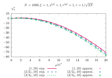
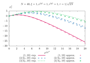
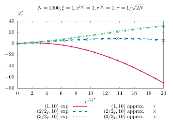
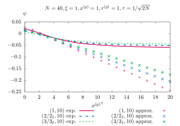
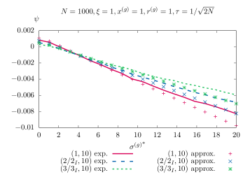
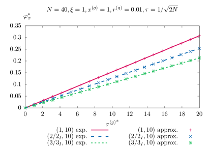
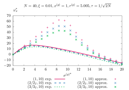
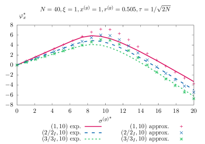
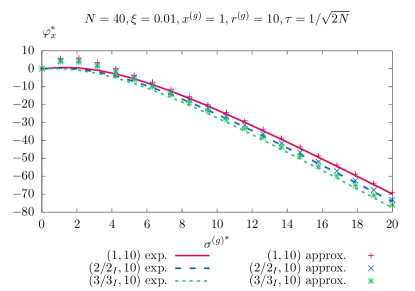
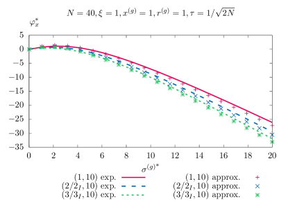
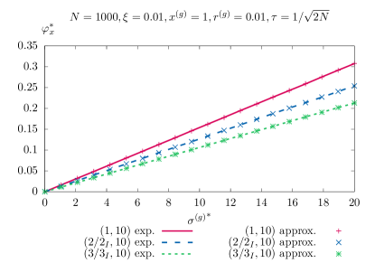
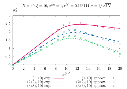
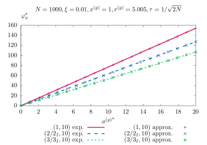
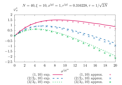
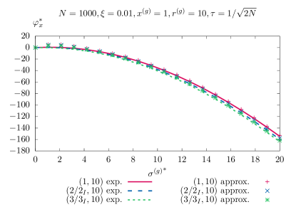
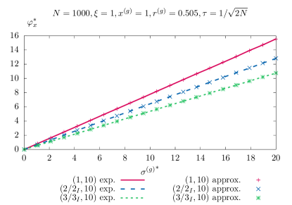
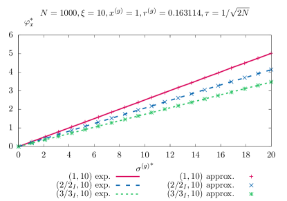
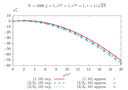
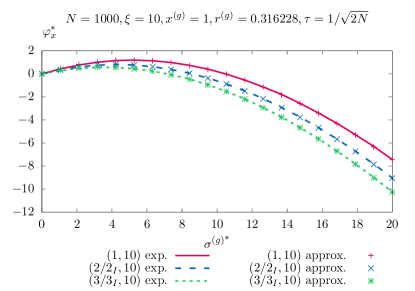
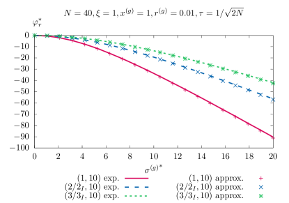
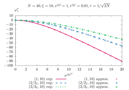
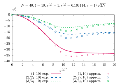
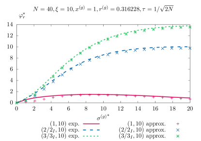
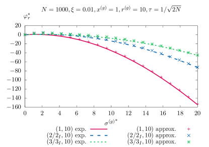
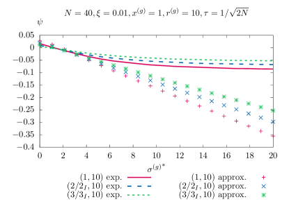
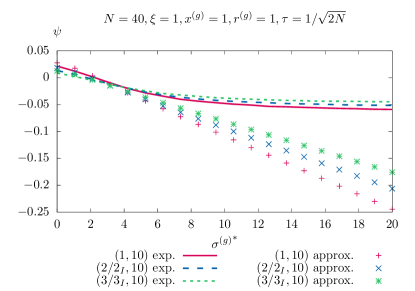
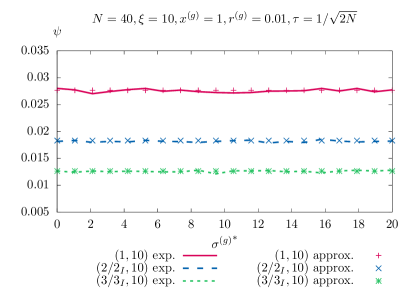
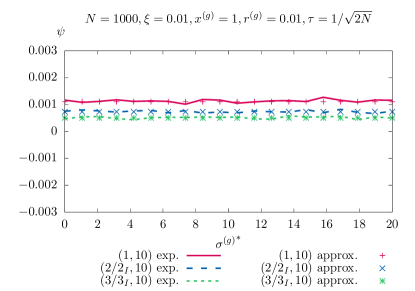
Figs. 3, 4, and 5 show plots comparing the derived closed-form approximation for $\varphi_{x}^{*}$, $\varphi_{r}^{*}$, and $\psi$, respectively, with one-generation experiments. The pluses, crosses, and stars have been calculated by evaluating Equation 38 with Equations 15, 20, and 37, Equation 44 with Equations 15 and 37, and Equation 54 with Equation 15, respectively. The solid, dashed, and dotted lines have been generated by one-generation experiments. For this, the generational loop has been run $10^{5}$ times for a fixed parental individual and constant parameters. The experimentally determined values for $\varphi_{x}^{*}$, $\varphi_{r}^{*}$, and $\psi$ from those $10^{5}$ runs have been averaged. Further figures showing comparisons for additional configurations are provided in the supplementary material (Figs. 10 to 18 in Appendix F).

Figure 5: Comparison of the SAR approximation with simulations.

IV-C The Evolution Dynamics in the Deterministic Approximation

IV-C1 The Evolution Equations

With the derived progress rates $\varphi_{x}^{*}$ and $\varphi_{r}^{*}$ and the SAR $\psi$ from Section IV-B, the approximated deterministic evolution equations can be iterated. By doing this, the dynamics can be predicted. The predictions by the approximations are compared to real runs of the ES. Using Equations 6 to 8 together with Equations 11 to 13, the evolution equations read

$$x^{(g+1)} =x^{(g)}-\frac{x^{(g)}{\varphi^{(g)}_{x}}^{*}}{N}=x^{(g)}\left(1-\frac{{\varphi^{(g)}_{x}}^{*}}{N}\right)$$ (55)

$$r^{(g+1)} =r^{(g)}-\frac{r^{(g)}{\varphi^{(g)}_{r}}^{*}}{N}=r^{(g)}\left(1-\frac{{\varphi^{(g)}_{r}}^{*}}{N}\right)$$ (56)

$$\sigma^{(g+1)} =\sigma^{(g)}+\sigma^{(g)}\psi^{(g)}=\sigma^{(g)}\left(1+\psi^{(g)}\right).$$ (57)

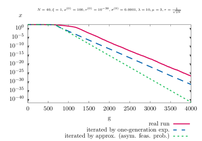
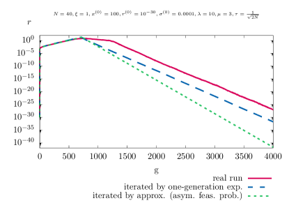
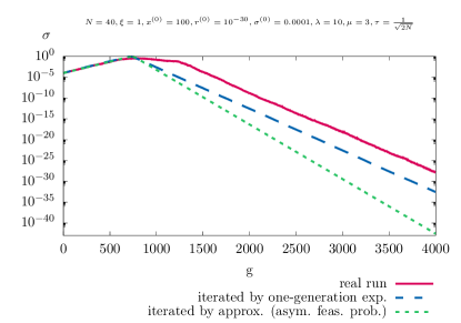
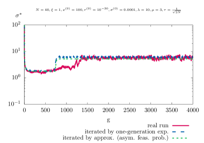
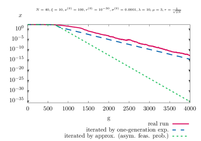
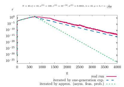
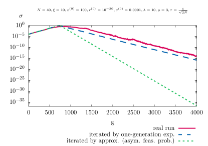
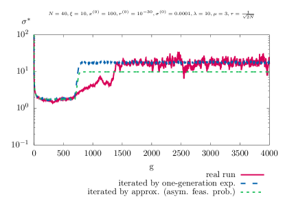
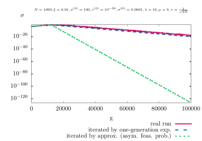
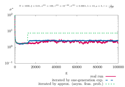
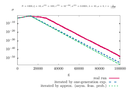
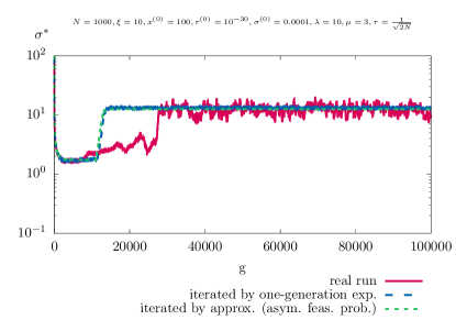
Fig. 6 shows the mean value dynamics of the $(3/3_{I},10)$-ES applied to the conically constrained problem for $N=1000$, $\xi=20$, and $\tau=\frac{1}{\sqrt{2N}}$. Additional figures for more configurations are provided in the supplementary material (Figs. 19, 20, 21, 22, 23, and 24 in Appendix F). The lines for the real runs have been generated by averaging $100$ real runs of the ES. The lines for the iteration by approximation have been computed by iterating the mean value iterative system with the derived approximations in Section IV-B for ${\varphi^{(g)}_{x}}^{*}$, ${\varphi^{(g)}_{r}}^{*}$, and $\psi^{(g)}$. Note that due to the approximations used it is possible that the iteration of the mean value iterative system yields infeasible $(x^{(g)},r^{(g)})^{T}$ in some generation $g$. If this situation has occurred, the corresponding $(x^{(g)},r^{(g)})^{T}$ have been projected back. Then, in the following iterations, the projected values have been used. This is what is indicated by the repair step in 21 to 23 of Algorithm 1 that is only needed for the iteration of the mean value iterative system.

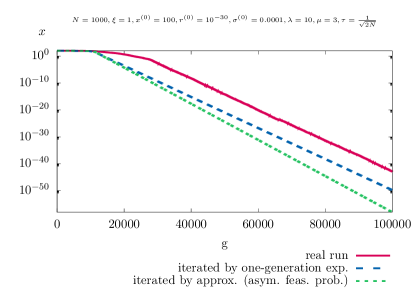
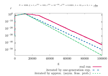
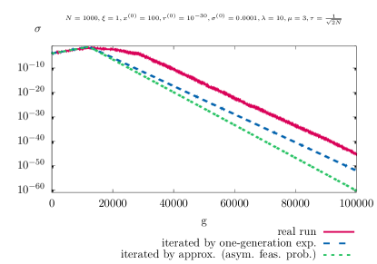
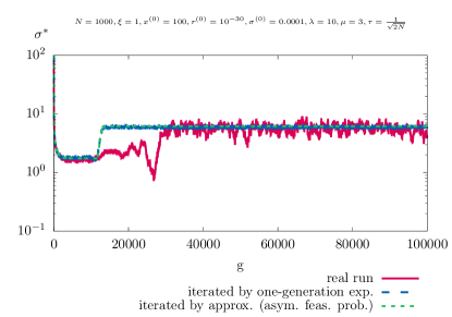
The stationary state is reached by the ES (solid line) later than predicted (dotted line). This can be seen in the first three subplots of Fig. 6. The slope of the lines coincides well between the prediction and the ES. But the lines are shifted for some number of generations. The same can be observed in the fourth subplot of Fig. 6 where the $\sigma^{*}$ steady state value is attained later by the ES (solid line) than predicted (dotted line). Further experiments to investigate this behavior (not shown here) showed that higher values of $\tau$ reduce this discrepancy by allowing larger $\sigma$-mutations.

Figure 6: Mean value dynamics closed-form approximation and real-run comparison of the $(3/3_{I},10)$-ES with repair by projection applied to the conically constrained problem ($N=1000$).

IV-C2 The ES in the Stationary State

The state of the $(\mu/\mu_{I},\lambda)$-ES on the conically constrained problem is completely described by $(x^{(g)},r^{(g)},\sigma^{(g)})^{T}$ (assuming constant exogenous parameters). For sufficiently large $g$, the ES transitions into a stationary state. On average, the normalized mutation strength should be constant in this steady state. That is, in the steady state the expectation of the normalized mutation strength $\sigma^{*}_{ss}$ is constant for large time scales

$$\sigma^{*}_{ss}:=\lim_{g\rightarrow\infty}\,{\sigma^{(g)}}^{*}.$$ (58)

Hence, for sufficiently large $g$, ${\sigma^{(g)}}^{*}={\sigma^{(g+1)}}^{*}=\sigma^{*}_{ss}$. Requiring this condition, a steady state condition can be derived. To this end, Equation 57 is normalized yielding

$$\frac{r^{(g+1)}{\sigma^{(g+1)}}^{*}}{N}=\frac{r^{(g)}{\sigma^{(g)}}^{*}}{N}\left(1+\psi^{(g)}\right).$$ (59)

Setting ${\sigma^{(g)}}^{*}={\sigma^{(g+1)}}^{*}$ results in

$$r^{(g+1)}=r^{(g)}\left(1+\psi^{(g)}\right).$$ (60)

Inserting Equation 56 yields the steady state condition

$$r^{(g)}\left(1-\frac{{\varphi^{(g)}_{r}}^{*}}{N}\right) =r^{(g)}\left(1+\psi^{(g)}\right)$$ (61)

$$1-\frac{{\varphi^{(g)}_{r}}^{*}}{N} =1+\psi^{(g)}$$ (62)

$$\frac{{\varphi^{(g)}_{r}}^{*}}{N} =-\psi^{(g)}.$$ (63)

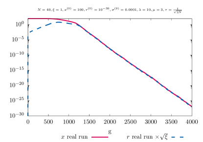
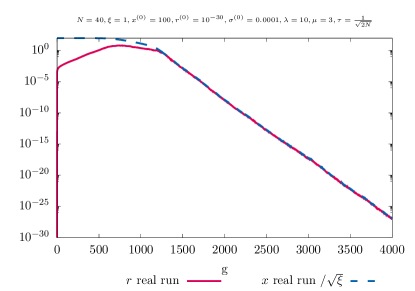
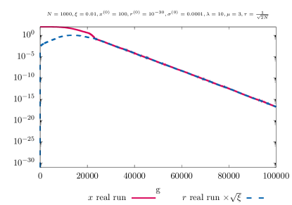
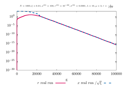
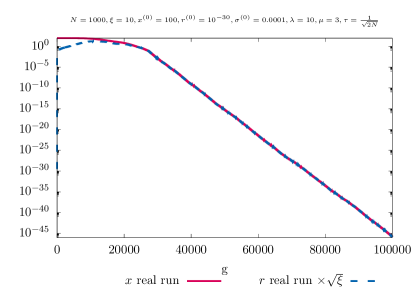
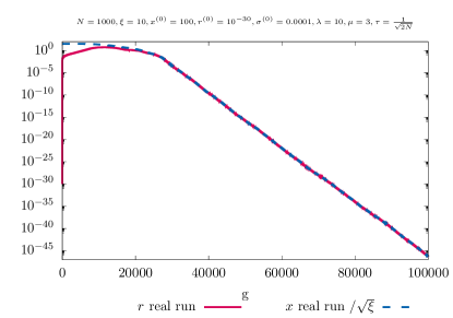
In the steady state, the ES moves in the vicinity of the cone boundary. This can be observed in real ES runs (see the third rows in Figs. 19, 20, 21, 22, 23, and 24 in the supplementary material Appendix F). Hence, for the derivation of analytical approximations for the steady state, the condition $P_{\text{feas}}\approx 0$ is assumed similar to the $(1,\lambda)$ case. However, in contrast to the $(1,\lambda)$ case, the assumption $\frac{x^{(g)}}{\sqrt{\xi}r^{(g)}}=1$ is too crude. There exists a distance from the cone boundary for some parameter configurations that cannot be neglected (this can for example be seen in the third row of Fig. 21 in the supplementary material Appendix F). Considering the distance ratio $r^{(g)}/x^{(g)}$, one observes that this ratio approaches a steady state value. This results in the condition

$$\frac{r^{(g)}}{x^{(g)}}=\frac{r^{(g+1)}}{x^{(g+1)}}$$ (64)

for sufficiently large values of $g$. Using the progress rates (Equations 9 to 12), this can be written as

$$\frac{r_{ss}}{x_{ss}}=\frac{r_{ss}\left(1-\frac{{\varphi_{r}}_{ss}^{*}}{N}\right)}{x_{ss}\left(1-\frac{{\varphi_{x}}_{ss}^{*}}{N}\right)},$$ (65)

which implies

$${\varphi_{r}}_{ss}^{*}={\varphi_{x}}_{ss}^{*}.$$ (66)

With the assumption $P_{\text{feas}}\approx 0$, use of the infeasible case approximations (Equation 37 and Equation D.303) for treating Equation 66 further, yields

$$\begin{multlined}N\bigg{(}1-\frac{x_{ss}}{\sqrt{\xi}r_{ss}}\left(1-\frac{{{\varphi_{x}^{*}}_{ss}}_{\text{infeas}}}{N}\right)\sqrt{\frac{1+\frac{{{\sigma_{ss}^{*}}}^{2}}{\mu N}}{1+\frac{{{\sigma_{ss}^{*}}}^{2}}{N}}}\bigg{)}={{\varphi_{x}^{*}}_{ss}}_{\text{infeas}}\end{multlined}N\bigg{(}1-\frac{x_{ss}}{\sqrt{\xi}r_{ss}}\left(1-\frac{{{\varphi_{x}^{*}}_{ss}}_{\text{infeas}}}{N}\right)\sqrt{\frac{1+\frac{{{\sigma_{ss}^{*}}}^{2}}{\mu N}}{1+\frac{{{\sigma_{ss}^{*}}}^{2}}{N}}}\bigg{)}={{\varphi_{x}^{*}}_{ss}}_{\text{infeas}}$$ (68)

$$\begin{multlined}N-\left(\frac{x_{ss}}{\sqrt{\xi}r_{ss}}\left(N-{{\varphi_{x}^{*}}_{ss}}_{\text{infeas}}\right)\sqrt{\frac{1+\frac{{{\sigma_{ss}^{*}}}^{2}}{\mu N}}{1+\frac{{{\sigma_{ss}^{*}}}^{2}}{N}}}\right)={{\varphi_{x}^{*}}_{ss}}_{\text{infeas}}.\end{multlined}N-\left(\frac{x_{ss}}{\sqrt{\xi}r_{ss}}\left(N-{{\varphi_{x}^{*}}_{ss}}_{\text{infeas}}\right)\sqrt{\frac{1+\frac{{{\sigma_{ss}^{*}}}^{2}}{\mu N}}{1+\frac{{{\sigma_{ss}^{*}}}^{2}}{N}}}\right)={{\varphi_{x}^{*}}_{ss}}_{\text{infeas}}.$$ (70)

Further,

$$\begin{multlined}\left(\frac{x_{ss}}{\sqrt{\xi}r_{ss}}\left(N-{{\varphi_{x}^{*}}_{ss}}_{\text{infeas}}\right)\sqrt{\frac{1+\frac{{{\sigma_{ss}^{*}}}^{2}}{\mu N}}{1+\frac{{{\sigma_{ss}^{*}}}^{2}}{N}}}\right)=\left(N-{{\varphi_{x}^{*}}_{ss}}_{\text{infeas}}\right)\end{multlined}\left(\frac{x_{ss}}{\sqrt{\xi}r_{ss}}\left(N-{{\varphi_{x}^{*}}_{ss}}_{\text{infeas}}\right)\sqrt{\frac{1+\frac{{{\sigma_{ss}^{*}}}^{2}}{\mu N}}{1+\frac{{{\sigma_{ss}^{*}}}^{2}}{N}}}\right)=\left(N-{{\varphi_{x}^{*}}_{ss}}_{\text{infeas}}\right)$$ (72)

$$\begin{multlined}\hskip 142.26378pt\frac{x_{ss}}{\sqrt{\xi}r_{ss}}=\frac{1}{\sqrt{\frac{1+\frac{{{\sigma_{ss}^{*}}}^{2}}{\mu N}}{1+\frac{{{\sigma_{ss}^{*}}}^{2}}{N}}}}\end{multlined}\hskip 142.26378pt\frac{x_{ss}}{\sqrt{\xi}r_{ss}}=\frac{1}{\sqrt{\frac{1+\frac{{{\sigma_{ss}^{*}}}^{2}}{\mu N}}{1+\frac{{{\sigma_{ss}^{*}}}^{2}}{N}}}}$$ (74)

follows. Considering Equation 66 for Equation 63 results in

$$\frac{{\varphi_{x}}^{*}_{ss}}{N}=-\psi_{ss}.$$ (75)

Assuming $P_{\text{feas}}\approx 0$, the approximations for the infeasible case can be used. Insertion of Equation 74 into Equation 37 with the assumption $\frac{1}{\xi}\frac{1+\frac{{{\sigma_{ss}^{*}}}^{2}}{2N}}{1+\frac{{{\sigma_{ss}^{*}}}^{2}}{N}}\simeq\frac{1}{\xi}$ for $N\rightarrow\infty$ yields

$$\begin{multlined}{\varphi_{x}^{*}}_{ss}\approx\frac{N}{1+\xi}\left(1-\sqrt{\frac{1+\frac{{{\sigma_{ss}^{*}}}^{2}}{\mu N}}{1+\frac{{{\sigma_{ss}^{*}}}^{2}}{N}}}\sqrt{1+\frac{{{\sigma_{ss}^{*}}}^{2}}{N}}\right)\\ +\frac{{\sigma_{ss}^{*}}c_{\mu/\mu,\lambda}}{\sqrt{1+\xi}}\sqrt{\frac{1+\frac{{{\sigma_{ss}^{*}}}^{2}}{\mu N}}{1+\frac{{{\sigma_{ss}^{*}}}^{2}}{N}}}\end{multlined}{\varphi_{x}^{*}}_{ss}\approx\frac{N}{1+\xi}\left(1-\sqrt{\frac{1+\frac{{{\sigma_{ss}^{*}}}^{2}}{\mu N}}{1+\frac{{{\sigma_{ss}^{*}}}^{2}}{N}}}\sqrt{1+\frac{{{\sigma_{ss}^{*}}}^{2}}{N}}\right)\\ +\frac{{\sigma_{ss}^{*}}c_{\mu/\mu,\lambda}}{\sqrt{1+\xi}}\sqrt{\frac{1+\frac{{{\sigma_{ss}^{*}}}^{2}}{\mu N}}{1+\frac{{{\sigma_{ss}^{*}}}^{2}}{N}}}$$ (78)

$$\begin{multlined}\phantom{{\varphi_{x}^{*}}_{ss}}=\frac{N}{1+\xi}\left(1-\sqrt{1+\frac{{{\sigma_{ss}^{*}}}^{2}}{\mu N}}\right)+\frac{{\sigma_{ss}^{*}}c_{\mu/\mu,\lambda}}{\sqrt{1+\xi}}\sqrt{\frac{1+\frac{{{\sigma_{ss}^{*}}}^{2}}{\mu N}}{1+\frac{{{\sigma_{ss}^{*}}}^{2}}{N}}}\end{multlined}\phantom{{\varphi_{x}^{*}}_{ss}}=\frac{N}{1+\xi}\left(1-\sqrt{1+\frac{{{\sigma_{ss}^{*}}}^{2}}{\mu N}}\right)+\frac{{\sigma_{ss}^{*}}c_{\mu/\mu,\lambda}}{\sqrt{1+\xi}}\sqrt{\frac{1+\frac{{{\sigma_{ss}^{*}}}^{2}}{\mu N}}{1+\frac{{{\sigma_{ss}^{*}}}^{2}}{N}}}$$ (80)

$$\begin{multlined}\phantom{{\varphi_{x}^{*}}_{ss}}\simeq\frac{N}{1+\xi}\left(1-\left(1+\frac{{{\sigma_{ss}^{*}}}^{2}}{2\mu N}\right)\right)+\frac{{\sigma_{ss}^{*}}c_{\mu/\mu,\lambda}}{\sqrt{1+\xi}}\end{multlined}\phantom{{\varphi_{x}^{*}}_{ss}}\simeq\frac{N}{1+\xi}\left(1-\left(1+\frac{{{\sigma_{ss}^{*}}}^{2}}{2\mu N}\right)\right)+\frac{{\sigma_{ss}^{*}}c_{\mu/\mu,\lambda}}{\sqrt{1+\xi}}$$ (82)

$$\begin{multlined}\phantom{{\varphi_{x}^{*}}_{ss}}=\frac{N}{1+\xi}\left(-\frac{{{\sigma_{ss}^{*}}}^{2}}{2\mu N}\right)+\frac{{\sigma_{ss}^{*}}c_{\mu/\mu,\lambda}}{\sqrt{1+\xi}}.\end{multlined}\phantom{{\varphi_{x}^{*}}_{ss}}=\frac{N}{1+\xi}\left(-\frac{{{\sigma_{ss}^{*}}}^{2}}{2\mu N}\right)+\frac{{\sigma_{ss}^{*}}c_{\mu/\mu,\lambda}}{\sqrt{1+\xi}}.$$ (84)

In the step from Equation 80 to Equation 82, it has been assumed that $\sqrt{\frac{1+\frac{{{\sigma_{ss}^{*}}}^{2}}{\mu N}}{1+\frac{{{\sigma_{ss}^{*}}}^{2}}{N}}}\simeq 1$ for $N\gg{\sigma_{ss}^{*}}^{2}$ and a Taylor expansion (neglecting the quadratic and higher order terms) has been applied to $\sqrt{1+\frac{{{\sigma_{ss}^{*}}}^{2}}{\mu N}}$. With Equation 84, the steady state equation Equation 63 reads for the asymptotic case of $N\rightarrow\infty$

$$\begin{multlined}\frac{1}{1+\xi}\left(-\frac{{{\sigma_{ss}^{*}}}^{2}}{2\mu N}\right)+\frac{{\sigma_{ss}^{*}}c_{\mu/\mu,\lambda}}{N\sqrt{1+\xi}}\\ \hskip 56.9055pt=-\tau^{2}\left(\frac{1}{2}+e_{\mu,\lambda}^{1,1}-\frac{{\sigma_{ss}^{*}}c_{\mu/\mu,\lambda}}{\sqrt{1+\xi}}\right).\end{multlined}\frac{1}{1+\xi}\left(-\frac{{{\sigma_{ss}^{*}}}^{2}}{2\mu N}\right)+\frac{{\sigma_{ss}^{*}}c_{\mu/\mu,\lambda}}{N\sqrt{1+\xi}}\\ \hskip 56.9055pt=-\tau^{2}\left(\frac{1}{2}+e_{\mu,\lambda}^{1,1}-\frac{{\sigma_{ss}^{*}}c_{\mu/\mu,\lambda}}{\sqrt{1+\xi}}\right).$$ (85)

Solving this quadratic equation yields the steady state normalized mutation strength (as the mutation strength is positive, the positive root is taken)

$$\begin{multlined}{\sigma_{ss}^{*}}=\sqrt{1+\xi}\mu c_{\mu/\mu,\lambda}\left[(1-N\tau^{2})+\right.\\ \left.\hskip 56.9055pt\sqrt{(1-N\tau^{2})^{2}+\frac{2\tau^{2}N\left(\frac{1}{2}+e_{\mu,\lambda}^{1,1}\right)}{\mu c_{\mu/\mu,\lambda}^{2}}}\right].\end{multlined}{\sigma_{ss}^{*}}=\sqrt{1+\xi}\mu c_{\mu/\mu,\lambda}\left[(1-N\tau^{2})+\right.\\ \left.\hskip 56.9055pt\sqrt{(1-N\tau^{2})^{2}+\frac{2\tau^{2}N\left(\frac{1}{2}+e_{\mu,\lambda}^{1,1}\right)}{\mu c_{\mu/\mu,\lambda}^{2}}}\right].$$ (86)

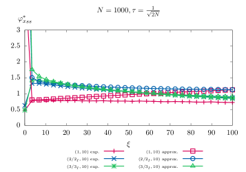
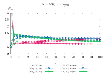
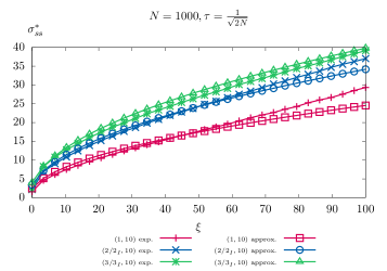
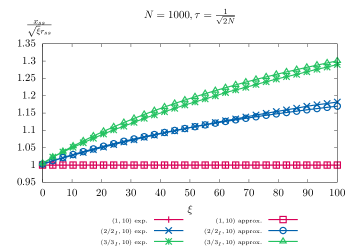
Fig. 7 shows plots of the steady state computations. The derived closed-form approximation has been compared to real ES runs. The values for visualizing the approximations have been calculated as follows. The steady state $\sigma^{*}_{ss}$ value has been computed by evaluating Equation 86. This value was then inserted into the derived approximations for the progress measures to obtain the values for ${\varphi_{x}^{*}}_{ss}$ and ${\varphi_{r}^{*}}_{ss}$. The values from experiments have been determined by computing the averages of the particular values in real ES runs. For this, the ES was run for $400N$ generations and the particular values have been averaged over these generations. This procedure was repeated $100$ times and those $100$ times have been averaged to compute the particular steady state values.

Figure 7: Steady state closed-form approximation and real-run comparison of the $(\mu/\mu_{I},\lambda)$-ES with repair by projection applied to the conically constrained problem.

V Results and Conclusions

A $(\mu/\mu_{I},\lambda)$-ES applied to a conically constrained problem has been theoretically analyzed.

Approximate expressions for the local progress measures and the SAR have been derived for asymptotic considerations. Comparison with numerical one-generation experiments shows the approximation quality. As can be seen in Fig. 3 and Fig. 4, the derived approximations for the $x$ and $r$ progress rates coincide well with the experiments, in particular for higher dimensions ($N=1000$). In the transition from the feasible to the infeasible case, the weighting with the offspring feasibility probability does not fit well in all the cases. This can be seen in the supplementary material (Figs. 10 to 15 in Appendix F). The middle row in these figures always shows a case between the feasible and the infeasible case. However, the deviation in these cases does not affect the steady state considerations because the ES moves in the vicinity of the cone boundary in the stationary state. The approximation for the SAR corresponds well to the experiments for small values of ${\sigma^{(g)}}^{*}$. It deviates for larger values of ${\sigma^{(g)}}^{*}$. Again, for higher $N$, the approximation quality fits better as can be seen in Fig. 5. This behavior is inherent in the SAR approximation. First, $N\gg{\sigma^{(g)}}^{*}$ has been assumed in deriving the SAR approximation. Second, quadratic and higher order terms have been neglected. Therefore, the SAR approximation is linear and hence necessarily deviates for large values of ${\sigma^{(g)}}^{*}$.

The approximate expressions for the local progress measures and the SAR derived for the $(\mu/\mu_{I},\lambda)$-ES generalize the results obtained for the $(1,\lambda)$-ES. Considering $\mu=1$ for Equation 20 and Equation 37 immediately results in [8, Eq. (3.120), p. 41] and [8, Eq. (3.149), p. 44], respectively, for the $x$ progress rate. For the $r$ progress rate, it is similar. Setting $\mu=1$ in Equation 44 results in [8, Eq. (3.221), p. 57] for the feasible case and in [8, Eq. (3.209), p. 56] for the infeasible case (after applying the definition of $\varphi^{*}$). The same holds for $\psi$. It only differs in the progress coefficients. It can easily be verified that Equation 54 with $\mu=1$ corresponds to [8, Eq. (3.281), p. 69].

For the macroscopic behavior, the local expected progress functions have been iterated to predict the mean value dynamics of the ES and analytic steady state expressions have been derived.

For the evolution dynamics, in Fig. 6 the rate of convergence from the prediction is very similar to the one exhibited by the real ES run. However, the theory predicts an earlier transitioning into the stationary state (see the fourth subplot of Fig. 6 showing the $\sigma^{*}$ dynamics). Further investigations (not shown here) showed that the fluctuations of the mean values obtained from real ES runs are such that the fluctuations cover the predictions. Larger values of $\tau$ reduce this discrepancy due to bigger $\sigma$-mutations.

The analytic steady state analysis resulted in a very interesting conclusion. It turns out that the astonishing result from the $(1,\lambda)$ case (see the derivations leading to [8, Eq. (3.308), p. 87]) extends to the multi-recombinative ES. One recognizes the equations for the sphere model in (86) (see [10, Eq. (4.11), p. 35]), i.e., Equation 86 can be written as

$$\sigma^{*}_{ss}=\sqrt{1+\xi}{\sigma^{*}_{ss}}_{\text{sphere}}$$ (87)

where ${\sigma^{*}_{ss}}_{\text{sphere}}$ denotes the steady state mutation strength value for the $(\mu/\mu_{I},\lambda)$-$\sigma$SA-ES applied to the sphere model. This means that in the steady state the $(\mu/\mu_{I},\lambda)$-$\sigma$SA-ES with repair by projection applied to the conically constrained problem moves towards the optimal value as if a sphere would be optimized. Additionally, the rate at which the ES approaches this optimal value is the same as if a sphere were to be optimized, independently of the value of $\xi$. The $x^{(g)}$ and $r^{(g)}$ dynamics are proportional to $\exp\left(-\frac{\varphi^{*}}{N}g\right)$ in the steady state. This follows from the definition of the progress rates $\varphi_{x}^{*}$ and $\varphi_{r}^{*}$. Consequently, linear convergence order with a convergence rate of $\frac{\varphi^{*}}{N}$ is implied. This means that the conically constrained problem has been turned into a sphere model by applying the projection as the repair method. However, the behavior is achieved by a $\sqrt{1+\xi}$ times larger mutation strength (87). That is, the ES performs larger search steps in the search space. These larger mutation steps are automatically realized by the self-adaptation as can be seen in (86).

The figure for the steady state (Fig. 7) allows for a comparison of the $(1,10)$-ES, the $(2/2_{I},10)$-ES, and the $(3/3_{I},10)$-ES. The mutation strength $\sigma_{ss}^{*}$ and $\frac{x_{ss}}{\sqrt{\xi}r_{ss}}$ ratio approximations come close to the ones determined by experiments. For the steady state progress rates, the approximations are not that good. The deviations are particularly high for small values of $\xi$. The reason for this is that in the derivations for $P_{Q}(q)$, $\xi$ has been assumed to be sufficiently large. Despite that, the figure gives insights. For the considered ESs, one can observe that the strategies with intermediate recombination exhibit faster progress in the steady state. The difference between the $(2/2_{I},10)$-ES and the $(3/3_{I},10)$-ES is marginal, which is also predicted by the theory as derived in the following. Based on Equation 84, one can compute the maximal $x$ progress in the steady state under the assumption $N\gg\sigma_{ss}^{*}$. Computing the first derivative with respect to $\sigma_{ss}^{*}$ of Equation 84 yields

$$\frac{\mathrm{d}}{\mathrm{d}\sigma_{ss}^{*}}{\varphi_{x}^{*}}_{ss}=\frac{c_{\mu/\mu,\lambda}}{\sqrt{1+\xi}}-\frac{\sigma_{ss}^{*}}{\mu(\sqrt{1+\xi})^{2}}$$ (88)

Setting Equation 88 to zero and solving for $\sigma_{ss}^{*}$ results in the mutation strength

$$\hat{\sigma}_{ss}^{*}=\sqrt{1+\xi}\mu c_{\mu/\mu,\lambda}$$ (89)

with which the maximal $x$ progress in the steady state is obtained. Further, by insertion of Equation 89 into Equation 84, the maximal $x$ progress follows as ${{}\hat{\varphi}_{x}^{*}}_{ss}(\mu,\lambda)=\frac{\mu c_{\mu/\mu,\lambda}^{2}}{2}$. Assuming it is achieved by the ES, ${{}\hat{\varphi}_{x}^{*}}_{ss}(2,10)\approx 1.61$ and ${{}\hat{\varphi}_{x}^{*}}_{ss}(3,10)\approx 1.70$ follow, which are relatively close to each other. In contrast to that, ${{}\hat{\varphi}_{x}^{*}}_{ss}(1,10)\approx 1.18$.

Insertion of Equation 89 into Equation 74 yields

$$\frac{\sqrt{\xi}r_{ss}}{x_{ss}}=\sqrt{\frac{1+\frac{(1+\xi)}{N}\mu c_{\mu/\mu,\lambda}^{2}}{1+\frac{(1+\xi)}{N}\mu c_{\mu/\mu,\lambda}^{2}\mu}}.$$ (90)

This gives insights about the deviation of the parental centroid from the cone boundary. Assuming $\frac{(1+\xi)}{N}\mu c_{\mu/\mu,\lambda}^{2}$ in Equation 90 to be sufficiently small, a Taylor expansion around $0$ for $\frac{(1+\xi)}{N}\mu c_{\mu/\mu,\lambda}^{2}$ can be applied. Together with subsequent cutoff after the linear term, it results in

$$\frac{\sqrt{\xi}r_{ss}}{x_{ss}}\simeq 1+\frac{(1+\xi)}{N}\frac{\mu c_{\mu/\mu,\lambda}^{2}}{2}(1-\mu).$$ (91)

As can be seen, in the case without recombination ($\mu=1$), the parental centroid moves on the cone boundary. However, with recombination ($\mu>1$), the centroid leaves this boundary and moves into the interior of the cone. The deviation from the cone boundary increases quadratically with $\mu$.

The theory developed allows further to compute the optimal value $\hat{\tau}$ for the learning parameter $\tau$. Requiring that the steady state mutation strength $\sigma_{ss}^{*}$ from (86) attains $\hat{\sigma}_{ss}^{*}$ from (89), one gets

$$\begin{multlined}\sqrt{1+\xi}\mu c_{\mu/\mu,\lambda}\stackrel{{\scriptstyle!}}{{=}}\sqrt{1+\xi}\mu c_{\mu/\mu,\lambda}\left[(1-N\tau^{2})+\right.\\ \left.\hskip 56.9055pt\sqrt{(1-N\tau^{2})^{2}+\frac{2\tau^{2}N\left(\frac{1}{2}+e_{\mu,\lambda}^{1,1}\right)}{\mu c_{\mu/\mu,\lambda}^{2}}}\right].\end{multlined}\sqrt{1+\xi}\mu c_{\mu/\mu,\lambda}\stackrel{{\scriptstyle!}}{{=}}\sqrt{1+\xi}\mu c_{\mu/\mu,\lambda}\left[(1-N\tau^{2})+\right.\\ \left.\hskip 56.9055pt\sqrt{(1-N\tau^{2})^{2}+\frac{2\tau^{2}N\left(\frac{1}{2}+e_{\mu,\lambda}^{1,1}\right)}{\mu c_{\mu/\mu,\lambda}^{2}}}\right].$$ (92)

Solving Equation 92 for $\tau$ yields the optimal learning parameter

$$\hat{\tau}(\mu,\lambda)=\frac{1}{\sqrt{2N}}\sqrt{\frac{\mu c_{\mu/\mu,\lambda}^{2}}{\mu c_{\mu/\mu,\lambda}^{2}-\frac{1}{2}-e_{\mu,\lambda}^{1,1}}},$$ (93)

which equals the optimal learning parameter of the sphere model (cf. [10, Eq. (4.116), p. 71]). For $\lambda\rightarrow\infty$ with $\mu/\lambda=\text{const.}$, one has $\hat{\tau}\simeq\frac{1}{\sqrt{2N}}$, which has been used in the simulations as an approximation to the optimal value. For $N=1000$, one has $\frac{1}{\sqrt{2N}}\approx 0.022$ and $\hat{\tau}(1,10)\approx 0.017$, $\hat{\tau}(2,10)\approx 0.021$, and $\hat{\tau}(3,10)\approx 0.022$. Hence, already for $\lambda=10$, $\frac{1}{\sqrt{2N}}$ approximates the optimal learning parameter relatively well.

Let us finally outline research goals to be addressed in the future. The analysis and comparison of different $\sigma$ control methods is a topic for future work. It is of interest to analyze the ES with cumulative step size adaptation (CSA) and Meta-ESs instead of self-adaptation for adapting $\sigma$. A comparison between the different approaches may give insights for practical recommendations of their application. As another research direction, it is of interest to investigate and compare different repair methods. Truncation and reflection are two examples. In the truncation approach, an infeasible offspring is repaired by the intersection of its mutation vector and the cone. For the reflection, infeasible offspring are mirrored into the feasible region about the cone boundary.

Patrick Spettel and Hans-Georg Beyer
Supplementary material

Appendix A Derivation of Closed-Form Expressions for the Projection

In this section, a geometrical approach for the projection of points that are outside of the feasible region onto the cone boundary is described. Fig. 8 shows a visualization of the 2D-plane spanned by an offspring $\tilde{\mathbf{x}}$ and the $x_{1}$ coordinate axis. The equation for the cone boundary is a direct consequence of the problem definition (Equation 2). The projected vector is indicated by $\mathbf{x}_{\Pi}$. The unit vectors $\mathbf{e}_{1}$, $\mathbf{e}_{\tilde{\mathbf{x}}}$, $\mathbf{e}_{\tilde{\mathbf{r}}}$, and $\mathbf{e}_{\tilde{\mathbf{c}}}$ are introduced. They are unit vectors in the direction of the $x_{1}$ axis, $\tilde{\mathbf{x}}$ vector, $\tilde{\mathbf{r}}=(0,\tilde{x}_{2},\ldots,\tilde{x}_{N})^{T}$ vector, and the cone boundary, respectively. The projection line is indicated by the dashed line. It indicates the shortest Euclidean distance from $\tilde{\mathbf{x}}$ to the cone boundary.

Figure 8: 2D-plane spanned by an offspring $\tilde{\mathbf{x}}$ and the $x_{1}$ coordinate axis. Vectors introduced for expressing the projection onto the feasible region of Fig. 1 are visualized. The vectors $\mathbf{e}_{1}$, $\mathbf{e}_{\tilde{\mathbf{x}}}$, $\mathbf{e}_{\tilde{\mathbf{r}}}$, and $\mathbf{e}_{\tilde{\mathbf{c}}}$ are unit vectors of the corresponding vectors. The dashed line indicates the orthogonal projection of $\tilde{\mathbf{x}}$ onto the cone boundary.

The goal is to compute the parameter vector after projection $\mathbf{x}_{\Pi}$. By inspecting Fig. 8 one can see that the projected vector $\mathbf{x}_{\Pi}$ can be expressed as

$$\mathbf{x}_{\Pi}=\begin{cases}(\mathbf{e}_{\tilde{\mathbf{c}}}^{T}\tilde{\mathbf{x}})\mathbf{e}_{\tilde{\mathbf{c}}}&\text{ if }\mathbf{e}_{\tilde{\mathbf{c}}}^{T}\tilde{\mathbf{x}}>0\\ \mathbf{0}&\text{ otherwise}.\end{cases}$$ (A.94)

From Equation 2, the equation of the cone boundary $\frac{x}{\sqrt{\xi}}$ follows. Using this, the vector $\mathbf{e}_{\tilde{\mathbf{c}}}$ can be expressed as a linear combination of the vectors $\mathbf{e}_{1}$ and $\mathbf{e}_{\tilde{\mathbf{r}}}$. After normalization (such that $||\mathbf{e}_{\tilde{\mathbf{c}}}||=1$) this writes

$$\mathbf{e}_{\tilde{\mathbf{c}}}=\frac{\mathbf{e}_{1}+\frac{1}{\sqrt{\xi}}\mathbf{e}_{\tilde{\mathbf{r}}}}{\sqrt{1+\frac{1}{\xi}}}.$$ (A.95)

The unit vectors $\mathbf{e}_{1}=(1,0,\ldots,0)^{T}$ and $\mathbf{e}_{\tilde{\mathbf{x}}}=\frac{\tilde{\mathbf{x}}}{||\mathbf{\tilde{\mathbf{x}}}||}$ are known. The vector $\mathbf{e}_{\tilde{\mathbf{r}}}$ is a unit vector in direction of $\tilde{\mathbf{x}}$ in the dimensions $2$ to $N$, i.e.,

$$\begin{split}\mathbf{e}_{\tilde{\mathbf{r}}}&=(0,(\tilde{\mathbf{x}})_{2},\ldots,(\tilde{\mathbf{x}})_{N})^{T}/||\tilde{\mathbf{r}}||.\end{split}$$ (A.96)

Inserting Equation A.96 into Equation A.95 results in

$$\mathbf{e}_{\tilde{\mathbf{c}}}=\left(1,\frac{(\tilde{\mathbf{x}})_{2}}{\sqrt{\xi}||\tilde{\mathbf{r}}||},\ldots,\frac{(\tilde{\mathbf{x}})_{N}}{\sqrt{\xi}||\tilde{\mathbf{r}}||}\right)^{T}\bigg{/}\sqrt{1+\frac{1}{\xi}}.$$ (A.97)

Using Equation A.97 it follows that

$$\begin{split}\mathbf{e}_{\tilde{\mathbf{c}}}^{T}\tilde{\mathbf{x}}&=\left((\tilde{\mathbf{x}})_{1}+\frac{(\tilde{\mathbf{x}})_{2}^{2}+\cdots+(\tilde{\mathbf{x}})_{N}^{2}}{\sqrt{\xi}||\tilde{\mathbf{r}}||}\right)\bigg{/}\sqrt{1+\frac{1}{\xi}}\\ &=\left((\tilde{\mathbf{x}})_{1}+\frac{||\tilde{\mathbf{r}}||^{2}}{\sqrt{\xi}||\tilde{\mathbf{r}}||}\right)\bigg{/}\sqrt{1+\frac{1}{\xi}}\\ &=\left((\tilde{\mathbf{x}})_{1}+\frac{||\tilde{\mathbf{r}}||}{\sqrt{\xi}}\right)\bigg{/}\sqrt{1+\frac{1}{\xi}}=\left((\tilde{\mathbf{x}})_{1}\sqrt{\xi}+||\tilde{\mathbf{r}}||\right)\big{/}\sqrt{\xi+1}.\end{split}$$ (A.98)

Use of Equations A.98, A.97, and A.94 yields for the case $\mathbf{e}_{\tilde{\mathbf{c}}}^{T}\tilde{\mathbf{x}}>0$

$$\begin{split}\mathbf{x}_{\Pi}&=(\mathbf{e}_{\tilde{\mathbf{c}}}^{T}\tilde{\mathbf{x}})\mathbf{e}_{\tilde{\mathbf{c}}}\\ &=\frac{1}{1+\frac{1}{\xi}}\left((\tilde{\mathbf{x}})_{1}+\frac{(\tilde{\mathbf{x}})_{2}^{2}+\cdots+(\tilde{\mathbf{x}})_{N}^{2}}{\sqrt{\xi}||\tilde{\mathbf{r}}||}\right)\left(1,\frac{(\tilde{\mathbf{x}})_{2}}{\sqrt{\xi}||\tilde{\mathbf{r}}||},\ldots,\frac{(\tilde{\mathbf{x}})_{N}}{\sqrt{\xi}||\tilde{\mathbf{r}}||}\right)^{T}.\end{split}$$ (A.99)

The first vector component of $\mathbf{x}_{\Pi}$ writes

$$\begin{split}q=(\mathbf{x}_{\Pi})_{1}&=\frac{1}{1+\frac{1}{\xi}}\left((\tilde{\mathbf{x}})_{1}+\frac{(\tilde{\mathbf{x}})_{2}^{2}+\cdots+(\tilde{\mathbf{x}})_{N}^{2}}{\sqrt{\xi}||\tilde{\mathbf{r}}||}\right)=\frac{\xi}{\xi+1}\left((\tilde{\mathbf{x}})_{1}+\frac{||\tilde{\mathbf{r}}||}{\sqrt{\xi}}\right).\end{split}$$ (A.100)

The $k$-th vector component of $\mathbf{x}_{\Pi}$ for $k\in\{2,\ldots,N\}$ writes

$$\begin{split}(\mathbf{x}_{\Pi})_{k}&=\frac{\xi}{\xi+1}\left((\tilde{\mathbf{x}})_{1}+\frac{||\tilde{\mathbf{r}}||}{\sqrt{\xi}}\right)\frac{(\tilde{\mathbf{x}})_{k}}{\sqrt{\xi}||\tilde{\mathbf{r}}||}=\frac{\xi}{\xi+1}\left(\frac{(\tilde{\mathbf{x}})_{1}}{\sqrt{\xi}||\tilde{\mathbf{r}}||}+\frac{1}{\xi}\right)(\tilde{\mathbf{x}})_{k}.\end{split}$$ (A.101)

And the projected distance from the cone axis $||\mathbf{r}_{\Pi}||$ writes

$$\begin{split}q_{r}=||\mathbf{r}_{\Pi}||&=\sqrt{\sum_{k=2}^{N}(\mathbf{x}_{\Pi})_{k}^{2}}=\sqrt{\sum_{k=2}^{N}\left(\frac{\xi}{\xi+1}\left(\frac{(\tilde{\mathbf{x}})_{1}}{\sqrt{\xi}||\tilde{\mathbf{r}}||}+\frac{1}{\xi}\right)\right)^{2}(\tilde{\mathbf{x}})_{k}^{2}}\\ &=\left(\frac{\xi}{\xi+1}\left(\frac{(\tilde{\mathbf{x}})_{1}}{\sqrt{\xi}||\tilde{\mathbf{r}}||}+\frac{1}{\xi}\right)\right)||\tilde{\mathbf{r}}||.\end{split}$$ (A.102)

Note that in terms of the $(x,r)^{T}$ representation, the offspring $\tilde{\mathbf{x}}$ can be expressed as $(\mathbf{e}_{1}^{T}\tilde{\mathbf{x}},\mathbf{e}_{\tilde{\mathbf{r}}}^{T}\tilde{\mathbf{x}})^{T}=((\tilde{\mathbf{x}})_{1},||\tilde{\mathbf{r}}||)^{T}$. This is exactly what is expected. The first component is the value in direction of the cone axis. The second component is the distance from the cone axis.

Appendix B Derivation of the Normal Approximation for the Offspring Density in $r$ Direction

From the offspring generation (7 and 8) it follows that the distance from the cone’s axis of the offspring is

$$\begin{split}\tilde{r}&=\sqrt{{r^{(g)}}^{2}+2\sigma^{(g)}r^{(g)}z_{2}+{\sigma^{(g)}}^{2}z_{2}^{2}+{\sigma^{(g)}}^{2}\sum_{k=3}^{N}z_{k}^{2}}.\end{split}$$ (B.103)

Now, $2\sigma^{(g)}r^{(g)}z_{2}+{\sigma^{(g)}}^{2}z_{2}^{2}$ and ${\sigma^{(g)}}^{2}\sum_{k=3}^{N}z_{k}^{2}$ are replaced with normally distributed expressions with mean values and standard deviations of the corresponding expressions. With the moments of the i.i.d. variables according to a standard normal distribution $z_{k}$, $\mathrm{E}[z_{k}]=0$, and $\mathrm{E}[z_{k}^{2}]=1$, the expected values $\mathrm{E}\left[2\sigma^{(g)}r^{(g)}z_{2}+{\sigma^{(g)}}^{2}z_{2}^{2}\right]={\sigma^{(g)}}^{2}$ and $\mathrm{E}\left[{\sigma^{(g)}}^{2}\sum_{k=3}^{N}z_{k}^{2}\right]={\sigma^{(g)}}^{2}(N-2)$ follow. The variances are computed as

$$\begin{split}\mathrm{Var}&\left[2\sigma^{(g)}{r^{(g)}}z_{2}+{\sigma^{(g)}}^{2}z_{2}^{2}\right]\\ &=\mathrm{E}\left[(2\sigma^{(g)}{r^{(g)}}z_{2}+{\sigma^{(g)}}^{2}z_{2}^{2})^{2}\right]-\mathrm{E}\left[2\sigma^{(g)}{r^{(g)}}z_{2}+{\sigma^{(g)}}^{2}z_{2}^{2}\right]^{2}\\ &=\mathrm{E}\left[4{\sigma^{(g)}}^{2}{r^{(g)}}^{2}z_{2}^{2}+4{\sigma^{(g)}}^{3}{r^{(g)}}z_{2}^{3}+{\sigma^{(g)}}^{4}z_{2}^{4}\right]-{\sigma^{(g)}}^{4}\\ &=4{\sigma^{(g)}}^{2}{r^{(g)}}^{2}+3{\sigma^{(g)}}^{4}-{\sigma^{(g)}}^{4}=4{\sigma^{(g)}}^{2}{r^{(g)}}^{2}+2{\sigma^{(g)}}^{4}\end{split}$$ (B.104)

and

$$\begin{split}\mathrm{Var}\left[{\sigma^{(g)}}^{2}\sum_{i=3}^{N}z_{i}^{2}\right]&={\sigma^{(g)}}^{4}\sum_{i=3}^{N}\mathrm{Var}\left[z_{i}^{2}\right]={\sigma^{(g)}}^{4}\sum_{i=3}^{N}\mathrm{E}\left[z_{i}^{4}\right]-\mathrm{E}\left[z_{i}^{2}\right]^{2}\\ &={\sigma^{(g)}}^{4}\sum_{i=3}^{N}2=2{\sigma^{(g)}}^{4}(N-2)\end{split}$$ (B.105)

where the moments of the i.i.d. variables according to a standard normal distribution $z_{i}$ $\mathrm{E}[z_{i}^{2}]=1$, $\mathrm{E}[z_{i}^{3}]=0$, and $\mathrm{E}[z_{i}^{4}]=3$ were used.

With these results, the normal approximation follows as

$$\begin{split}\tilde{r}&\approx\sqrt{{r^{(g)}}^{2}+\mathcal{N}({\sigma^{(g)}}^{2},4{\sigma^{(g)}}^{2}{r^{(g)}}^{2}+2{\sigma^{(g)}}^{4})+\mathcal{N}({\sigma^{(g)}}^{2}(N-2),2{\sigma^{(g)}}^{4}(N-2))}\\ &=\sqrt{{r^{(g)}}^{2}+{\sigma^{(g)}}^{2}(N-1)+\sqrt{4{\sigma^{(g)}}^{2}{r^{(g)}}^{2}+2{\sigma^{(g)}}^{4}(N-1)}\mathcal{N}(0,1).}\end{split}$$ (B.106)

Substitution of the normalized quantity ${\sigma^{(g)}}^{*}=\frac{\sigma^{(g)}N}{{r^{(g)}}}$ yields after simplification

$$\tilde{r} \approx{r^{(g)}}\sqrt{1+\frac{{{\sigma^{(g)}}^{*}}^{2}}{N}\left(1-\frac{1}{N}\right)}\sqrt{1+\frac{2{\sigma^{(g)}}^{*}}{N}\frac{\sqrt{1+\frac{{{\sigma^{(g)}}^{*}}^{2}}{2N}\left(1-\frac{1}{N}\right)}}{1+\frac{{{\sigma^{(g)}}^{*}}^{2}}{N}\left(1-\frac{1}{N}\right)}\mathcal{N}(0,1)}.$$ (B.107)

As the expression $\frac{2{\sigma^{(g)}}^{*}}{N}\frac{\sqrt{1+\frac{{{\sigma^{(g)}}^{*}}^{2}}{2N}\left(1-\frac{1}{N}\right)}}{1+\frac{{{\sigma^{(g)}}^{*}}^{2}}{N}\left(1-\frac{1}{N}\right)}\mathcal{N}(0,1)\rightarrow 0$ with $N\rightarrow\infty$ (${\sigma^{(g)}}^{*}<\infty$), a further asymptotically simplified expression can be obtained by Taylor expansion of the square root at $0$ and cutoff after the linear term

$$\begin{split}\tilde{r}&\approx\underbrace{{r^{(g)}}\sqrt{1+\frac{{{\sigma^{(g)}}^{*}}^{2}}{N}\left(1-\frac{1}{N}\right)}}_{\bar{r}}+\underbrace{{r^{(g)}}\frac{{\sigma^{(g)}}^{*}}{N}\sqrt{\frac{1+\frac{{{\sigma^{(g)}}^{*}}^{2}}{2N}\left(1-\frac{1}{N}\right)}{1+\frac{{{\sigma^{(g)}}^{*}}^{2}}{N}\left(1-\frac{1}{N}\right)}}}_{\sigma_{r}}\mathcal{N}(0,1).\end{split}$$ (B.108)

Consequently, the mean of the asymptotic normal approximation of $\tilde{r}$ is $\bar{r}$ and its standard deviation is $\sigma_{r}$

$$\begin{split}p_{r}(r)&\approx\frac{1}{\sigma_{r}}\phi\left(\frac{r-\bar{r}}{\sigma_{r}}\right)=\frac{1}{\sqrt{2\pi}\sigma_{r}}\exp\left[-\frac{1}{2}\left(\frac{r-\bar{r}}{\sigma_{r}}\right)^{2}\right].\end{split}$$ (B.109)

Appendix C Derivation of $\mathrm{E}[\langle q\rangle]$

With 19, 17, and 13 of Algorithm 1,

$$\mathrm{E}[\langle q\rangle\,|\,x^{(g)}, r^{(g)},\sigma^{(g)}]:=\mathrm{E}[\langle q\rangle]$$ (C.110)

$$=\mathrm{E}\left[\frac{1}{\mu}\sum_{m=1}^{\mu}q_{m;\lambda}\,|\,x^{(g)},r^{(g)},\sigma^{(g)}\right]$$ (C.111)

$$=\frac{1}{\mu}\sum_{m=1}^{\mu}\mathrm{E}\left[q_{m;\lambda}\,|\,x^{(g)},r^{(g)},\sigma^{(g)}\right]$$ (C.112)

follows. This means that the expectation of $q_{m;\lambda}$, i.e., the $x$ value after (possible) projection of the $m$-th best offspring, is needed for the derivation of the progress rate in $x$ direction

$$\mathrm{E}[q_{m;\lambda}\,|\,x^{(g)},r^{(g)},\sigma^{(g)}] :=\mathrm{E}[q_{m;\lambda}]$$ (C.113)

$$=\int_{q=0}^{q=\infty}q\,p_{q_{m;\lambda}}(q)\,\mathrm{d}q$$ (C.114)

$$=\int_{q=0}^{q=\infty}q\,\frac{\lambda!}{(\lambda-m)!(m-1)!}p_{Q}(q)[1-P_{Q}(q)]^{\lambda-m}[P_{Q}(q)]^{m-1}\,\mathrm{d}q.$$ (C.115)

Equation C.114 follows directly from the definition of expectation where

$$p_{q_{m;\lambda}}(q):=p_{q_{m;\lambda}}(q\,|\,x^{(g)},r^{(g)},\sigma^{(g)})$$

indicates the probability density function of the $m$-th best (offspring with $m$-th smallest $q$ value) offspring’s $q$ value. The random variable $Q$ denotes the random $x$ values after projection. The step to Equation C.115 follows from the calculation of $p_{q_{m;\lambda}}(q)$. Because the objective function (Equation 1) is defined to return an individual’s $x$ value, $p_{q_{m;\lambda}}(q)$ is the probability density function of the $m$-th smallest $q$ value among $\lambda$ values. This calculation is well-known in order statistics (see, e.g., Arnold1992OrderStatisticsAPP). A short derivation is presented here for the case under consideration. A single offspring’s $q$ value has a probability density of $p_{Q}(q)$. In order for this particular $q$ value to be the $m$-th smallest, there must be $(\lambda-m)$ offspring greater than that, and $(m-1)$ offspring smaller. This results in the density $p_{Q}(q)[1-P_{Q}(q)]^{\lambda-m}[P_{Q}(q)]^{m-1}$ where $P_{Q}(q)=\mathrm{Pr}[Q\leq q]$. Because the number of such combinations is $\lambda\binom{\lambda-1}{m-1}=\frac{\lambda!}{(\lambda-m)!(m-1)!}$ one obtains

$$p_{q_{m;\lambda}}(q)=\frac{\lambda!}{(\lambda-m)!(m-1)!}p_{Q}(q)[1-P_{Q}(q)]^{\lambda-m}[P_{Q}(q)]^{m-1}.$$ (C.116)

Insertion of Equation C.115 into Equation C.112 results in

$$\mathrm{E}[\langle q\rangle] =\frac{1}{\mu}\sum_{m=1}^{\mu}\int_{q=0}^{q=\infty}q\,\frac{\lambda!}{(\lambda-m)!(m-1)!}p_{Q}(q)[1-P_{Q}(q)]^{\lambda-m}[P_{Q}(q)]^{m-1}$$ (C.117)

$$=\frac{\lambda!}{\mu}\int_{q=0}^{q=\infty}q\,p_{Q}(q)\sum_{m=1}^{\mu}\frac{[1-P_{Q}(q)]^{\lambda-m}[P_{Q}(q)]^{m-1}}{(\lambda-m)!(m-1)!}.$$ (C.118)

The identity

$$\sum_{m=1}^{\mu}\frac{P^{m-1}[1-P]^{\lambda-m}}{(m-1)!(\lambda-m)!}=\frac{1}{(\lambda-\mu-1)!(\mu-1)!}\int_{0}^{1-P}z^{\lambda-\mu-1}(1-z)^{\mu-1}\,\mathrm{d}z$$ (C.119)

stated in [Eq. (5.14), p. 147]Beyer2001APP allows expressing the sum in Equation C.118 as an integral. Application of Equation C.119 to Equation C.118 and expressing the fraction using the binomial coefficient yields

$$\mathrm{E}[\langle q\rangle]=(\lambda-\mu)\binom{\lambda}{\mu}\int_{q=0}^{q=\infty}q\,p_{Q}(q)\int_{z=0}^{z=1-P_{Q}(q)}z^{\lambda-\mu-1}(1-z)^{\mu-1}\,\mathrm{d}z\,\mathrm{d}q.$$ (C.120)

To proceed further, $z=1-P_{Q}(y)$ is substituted in the inner integral. This implies $y=P_{Q}^{-1}(1-z)$ and $\mathrm{d}z=-p_{Q}(y)$. The upper and lower bounds for the substituted integral follow as $y_{u}=P_{Q}^{-1}(1-1+P_{Q}(q))=q$ and $y_{l}=P_{Q}^{-1}(1-0)=\infty$, respectively. Therefore, one obtains

$$\mathrm{E} [\langle q\rangle]$$

$$=(\lambda-\mu)\binom{\lambda}{\mu}\int_{q=0}^{q=\infty}q\,p_{Q}(q)\int_{y=\infty}^{y=q}[1-P_{Q}(y)]^{\lambda-\mu-1}[P_{Q}(y)]^{\mu-1}(-p_{Q}(y))\,\mathrm{d}y\,\mathrm{d}q$$ (C.121)

$$=(\lambda-\mu)\binom{\lambda}{\mu}\int_{q=0}^{q=\infty}q\,p_{Q}(q)\int_{y=q}^{y=\infty}p_{Q}(y)[1-P_{Q}(y)]^{\lambda-\mu-1}[P_{Q}(y)]^{\mu-1}\,\mathrm{d}y\,\mathrm{d}q.$$ (C.122)

Changing the order of integration, one finally gets

$$\mathrm{E}[\langle q\rangle]=(\lambda-\mu)\binom{\lambda}{\mu}\int_{y=0}^{y=\infty}p_{Q}(y)[1-P_{Q}(y)]^{\lambda-\mu-1}[P_{Q}(y)]^{\mu-1}\int_{q=0}^{q=y}q\,p_{Q}(q)\,\mathrm{d}q\,\mathrm{d}y.$$ (C.123)

Approximations for $P_{Q}(q)$ and $p_{Q}(q)$ have been derived in [Sec. 3.1.2.1.2, pp. 21-39]SpettelBeyer2018SigmaSaEsConeAPP

$${P_{Q}}_{\text{feas}}(q):=\Phi\left(\frac{q-x^{(g)}}{\sigma^{(g)}}\right),\text{ for }q>\bar{r}\sqrt{\xi}$$ (C.124)

$${P_{Q}}_{\text{infeas}}(q):=\Phi\left(\frac{(1+1/\xi)q-x^{(g)}-\bar{r}/\sqrt{\xi}}{\sqrt{{\sigma^{(g)}}^{2}+\sigma_{r}^{2}/\xi}}\right),\text{ otherwise}.$$ (C.125)

Taking the derivative with respect to $q$ yields

$${p_{Q}}_{\text{feas}}(q)=\frac{1}{\sqrt{2\pi}\sigma^{(g)}}e^{-\frac{1}{2}\left(\frac{q-x^{(g)}}{\sigma^{(g)}}\right)^{2}},\text{ for }q>\bar{r}\sqrt{\xi}$$ (C.126)

$$\begin{multlined}{p_{Q}}_{\text{infeas}}(q)=\left(\frac{(1+1/\xi)}{\sqrt{{\sigma^{(g)}}^{2}+\sigma_{r}^{2}/\xi}}\right)\\ \times\frac{1}{\sqrt{2\pi}}\exp\left[-\frac{1}{2}\left(\frac{(1+1/\xi)q-x^{(g)}-\bar{r}/\sqrt{\xi}}{\sqrt{{\sigma^{(g)}}^{2}+\sigma_{r}^{2}/\xi}}\right)^{2}\right],\\ \text{ otherwise}.\end{multlined}{p_{Q}}_{\text{infeas}}(q)=\left(\frac{(1+1/\xi)}{\sqrt{{\sigma^{(g)}}^{2}+\sigma_{r}^{2}/\xi}}\right)\\ \times\frac{1}{\sqrt{2\pi}}\exp\left[-\frac{1}{2}\left(\frac{(1+1/\xi)q-x^{(g)}-\bar{r}/\sqrt{\xi}}{\sqrt{{\sigma^{(g)}}^{2}+\sigma_{r}^{2}/\xi}}\right)^{2}\right],\\ \text{ otherwise}.$$ (C.130)

They are used to proceed further. Two cases (being feasible with overwhelming probability and being infeasible with overwhelming probability) have been distinguished in the derivation of the $P_{Q}$ and $p_{Q}$. Therefore, those two cases are treated separately for Equation C.123.

C-A Derivation of ${\mathrm{E}[\langle q\rangle]}_{\text{feas}}$

For treating the feasible case, insertion of Equations C.124 and C.126 into Equation C.123 yields

$$\begin{multlined}\mathrm{E}[{\langle q\rangle}_{\text{feas}}]\approx(\lambda-\mu)\binom{\lambda}{\mu}\int_{y=0}^{y=\infty}{p_{Q}}_{\text{feas}}(y)[1-{P_{Q}}_{\text{feas}}(y)]^{\lambda-\mu-1}[{P_{Q}}_{\text{feas}}(y)]^{\mu-1}\\ \times\int_{q=0}^{q=y}q\,{p_{Q}}_{\text{feas}}(q)\,\mathrm{d}q\,\mathrm{d}y\end{multlined}\mathrm{E}[{\langle q\rangle}_{\text{feas}}]\approx(\lambda-\mu)\binom{\lambda}{\mu}\int_{y=0}^{y=\infty}{p_{Q}}_{\text{feas}}(y)[1-{P_{Q}}_{\text{feas}}(y)]^{\lambda-\mu-1}[{P_{Q}}_{\text{feas}}(y)]^{\mu-1}\\ \times\int_{q=0}^{q=y}q\,{p_{Q}}_{\text{feas}}(q)\,\mathrm{d}q\,\mathrm{d}y$$ (C.133)

$$\begin{multlined}\phantom{\mathrm{E}[{\langle q\rangle}_{\text{feas}}]}=(\lambda-\mu)\binom{\lambda}{\mu}\int_{y=\bar{r}\sqrt{\xi}}^{y=\infty}\frac{1}{\sqrt{2\pi}\sigma^{(g)}}e^{-\frac{1}{2}\left(\frac{y-x^{(g)}}{\sigma^{(g)}}\right)^{2}}\left[1-\Phi\left(\frac{y-x^{(g)}}{\sigma^{(g)}}\right)\right]^{\lambda-\mu-1}\\ \times\left[\Phi\left(\frac{y-x^{(g)}}{\sigma^{(g)}}\right)\right]^{\mu-1}\int_{q=\bar{r}\sqrt{\xi}}^{q=y}q\,\frac{1}{\sqrt{2\pi}\sigma^{(g)}}e^{-\frac{1}{2}\left(\frac{q-x^{(g)}}{\sigma^{(g)}}\right)^{2}}\,\mathrm{d}q\,\mathrm{d}y.\end{multlined}\phantom{\mathrm{E}[{\langle q\rangle}_{\text{feas}}]}=(\lambda-\mu)\binom{\lambda}{\mu}\int_{y=\bar{r}\sqrt{\xi}}^{y=\infty}\frac{1}{\sqrt{2\pi}\sigma^{(g)}}e^{-\frac{1}{2}\left(\frac{y-x^{(g)}}{\sigma^{(g)}}\right)^{2}}\left[1-\Phi\left(\frac{y-x^{(g)}}{\sigma^{(g)}}\right)\right]^{\lambda-\mu-1}\\ \times\left[\Phi\left(\frac{y-x^{(g)}}{\sigma^{(g)}}\right)\right]^{\mu-1}\int_{q=\bar{r}\sqrt{\xi}}^{q=y}q\,\frac{1}{\sqrt{2\pi}\sigma^{(g)}}e^{-\frac{1}{2}\left(\frac{q-x^{(g)}}{\sigma^{(g)}}\right)^{2}}\,\mathrm{d}q\,\mathrm{d}y.$$ (C.136)

For solving the inner integral, $t:=\frac{q-x^{(g)}}{\sigma^{(g)}}$ is substituted. It implies $q=\sigma^{(g)}t+x^{(g)}$ and $\mathrm{d}q=\sigma^{(g)}\,\mathrm{d}t$. The lower bound follows with $\sigma$-normalization, assuming $N\rightarrow\infty$, $N\gg{\sigma^{*}}^{(g)}$, and knowing that $x^{(g)}\geq\bar{r}\sqrt{\xi}$ holds for the feasible case. It reads

$$t_{l}=\frac{\bar{r}\sqrt{\xi}-x^{(g)}}{\sigma^{(g)}}=\frac{N}{{\sigma^{*}}^{(g)}}\frac{\bar{r}\sqrt{\xi}-x^{(g)}}{r^{(g)}}\simeq-\infty.$$

The application of the substitution results in

$$\int_{q=\bar{r}\sqrt{\xi}}^{q=y} q\,\frac{1}{\sqrt{2\pi}\sigma^{(g)}}e^{-\frac{1}{2}\left(\frac{q-x^{(g)}}{\sigma^{(g)}}\right)^{2}}\,\mathrm{d}q$$

$$\simeq\int_{t=-\infty}^{t=\frac{y-x^{(g)}}{\sigma^{(g)}}}(\sigma^{(g)}t+x^{(g)})\frac{1}{\sqrt{2\pi}\sigma^{(g)}}e^{-\frac{1}{2}t^{2}}\sigma^{(g)}\mathrm{d}t$$ (C.137)

$$=\sigma^{(g)}\frac{1}{\sqrt{2\pi}}\int_{t=-\infty}^{t=\frac{y-x^{(g)}}{\sigma^{(g)}}}t\,e^{-\frac{1}{2}t^{2}}\mathrm{d}t+x^{(g)}\int_{t=-\infty}^{t=\frac{y-x^{(g)}}{\sigma^{(g)}}}\frac{1}{\sqrt{2\pi}}e^{-\frac{1}{2}t^{2}}\mathrm{d}t.$$ (C.138)

The integral in the second summand in Equation C.138 can be expressed using the cumulative distribution function of the normal distribution $\Phi(\cdot)$. The integral in the first summand in Equation C.138 can be solved using the identity

$$\int_{-\infty}^{x}t\,e^{-\frac{1}{2}t^{2}}\,\mathrm{d}t=-e^{-\frac{1}{2}x^{2}}$$ (C.139)

derived in [Eq. (A.16), p. 331]Beyer2001APP. Hence, one obtains

$$\int_{q=\bar{r}\sqrt{\xi}}^{q=y} q\,\frac{1}{\sqrt{2\pi}\sigma^{(g)}}e^{-\frac{1}{2}\left(\frac{q-x^{(g)}}{\sigma^{(g)}}\right)^{2}}\,\mathrm{d}q\simeq x^{(g)}\Phi\left(\frac{y-x^{(g)}}{\sigma^{(g)}}\right)-\sigma^{(g)}\frac{1}{\sqrt{2\pi}}e^{-\frac{1}{2}\left(\frac{y-x^{(g)}}{\sigma^{(g)}}\right)^{2}}.$$ (C.140)

Equation C.140 can now be inserted into Equation C.136 yielding

$$\begin{multlined}\mathrm{E}[{\langle q\rangle}_{\text{feas}}]\approx(\lambda-\mu)\binom{\lambda}{\mu}\int_{y=\bar{r}\sqrt{\xi}}^{y=\infty}\frac{1}{\sqrt{2\pi}\sigma^{(g)}}e^{-\frac{1}{2}\left(\frac{y-x^{(g)}}{\sigma^{(g)}}\right)^{2}}\left[1-\Phi\left(\frac{y-x^{(g)}}{\sigma^{(g)}}\right)\right]^{\lambda-\mu-1}\\ \times\left[\Phi\left(\frac{y-x^{(g)}}{\sigma^{(g)}}\right)\right]^{\mu-1}x^{(g)}\Phi\left(\frac{y-x^{(g)}}{\sigma^{(g)}}\right)\,\mathrm{d}y\\ -(\lambda-\mu)\binom{\lambda}{\mu}\int_{y=\bar{r}\sqrt{\xi}}^{y=\infty}\frac{1}{\sqrt{2\pi}\sigma^{(g)}}e^{-\frac{1}{2}\left(\frac{y-x^{(g)}}{\sigma^{(g)}}\right)^{2}}\left[1-\Phi\left(\frac{y-x^{(g)}}{\sigma^{(g)}}\right)\right]^{\lambda-\mu-1}\\ \times\left[\Phi\left(\frac{y-x^{(g)}}{\sigma^{(g)}}\right)\right]^{\mu-1}\sigma^{(g)}\frac{1}{\sqrt{2\pi}}e^{-\frac{1}{2}\left(\frac{y-x^{(g)}}{\sigma^{(g)}}\right)^{2}}\,\mathrm{d}y.\end{multlined}\mathrm{E}[{\langle q\rangle}_{\text{feas}}]\approx(\lambda-\mu)\binom{\lambda}{\mu}\int_{y=\bar{r}\sqrt{\xi}}^{y=\infty}\frac{1}{\sqrt{2\pi}\sigma^{(g)}}e^{-\frac{1}{2}\left(\frac{y-x^{(g)}}{\sigma^{(g)}}\right)^{2}}\left[1-\Phi\left(\frac{y-x^{(g)}}{\sigma^{(g)}}\right)\right]^{\lambda-\mu-1}\\ \times\left[\Phi\left(\frac{y-x^{(g)}}{\sigma^{(g)}}\right)\right]^{\mu-1}x^{(g)}\Phi\left(\frac{y-x^{(g)}}{\sigma^{(g)}}\right)\,\mathrm{d}y\\ -(\lambda-\mu)\binom{\lambda}{\mu}\int_{y=\bar{r}\sqrt{\xi}}^{y=\infty}\frac{1}{\sqrt{2\pi}\sigma^{(g)}}e^{-\frac{1}{2}\left(\frac{y-x^{(g)}}{\sigma^{(g)}}\right)^{2}}\left[1-\Phi\left(\frac{y-x^{(g)}}{\sigma^{(g)}}\right)\right]^{\lambda-\mu-1}\\ \times\left[\Phi\left(\frac{y-x^{(g)}}{\sigma^{(g)}}\right)\right]^{\mu-1}\sigma^{(g)}\frac{1}{\sqrt{2\pi}}e^{-\frac{1}{2}\left(\frac{y-x^{(g)}}{\sigma^{(g)}}\right)^{2}}\,\mathrm{d}y.$$ (C.145)

The first term in Equation C.145 can be simplified by using ${P_{Q}}_{\text{feas}}(y)=\Phi\left(\frac{y-x^{(g)}}{\sigma^{(g)}}\right)$. It yields

$$\begin{multlined}(\lambda-\mu)\binom{\lambda}{\mu}\int_{y=\bar{r}\sqrt{\xi}}^{y=\infty}\frac{1}{\sqrt{2\pi}\sigma^{(g)}}e^{-\frac{1}{2}\left(\frac{y-x^{(g)}}{\sigma^{(g)}}\right)^{2}}\left[1-\Phi\left(\frac{y-x^{(g)}}{\sigma^{(g)}}\right)\right]^{\lambda-\mu-1}\\ \times\left[\Phi\left(\frac{y-x^{(g)}}{\sigma^{(g)}}\right)\right]^{\mu-1}x^{(g)}\Phi\left(\frac{y-x^{(g)}}{\sigma^{(g)}}\right)\,\mathrm{d}y\end{multlined}(\lambda-\mu)\binom{\lambda}{\mu}\int_{y=\bar{r}\sqrt{\xi}}^{y=\infty}\frac{1}{\sqrt{2\pi}\sigma^{(g)}}e^{-\frac{1}{2}\left(\frac{y-x^{(g)}}{\sigma^{(g)}}\right)^{2}}\left[1-\Phi\left(\frac{y-x^{(g)}}{\sigma^{(g)}}\right)\right]^{\lambda-\mu-1}\\ \times\left[\Phi\left(\frac{y-x^{(g)}}{\sigma^{(g)}}\right)\right]^{\mu-1}x^{(g)}\Phi\left(\frac{y-x^{(g)}}{\sigma^{(g)}}\right)\,\mathrm{d}y$$ (C.148)

$$\begin{multlined}=x^{(g)}(\lambda-\mu)\binom{\lambda}{\mu}\int_{y=\bar{r}\sqrt{\xi}}^{y=\infty}{p_{Q}}_{\text{feas}}(y)[1-{P_{Q}}_{\text{feas}}(y)]^{\lambda-\mu-1}[{P_{Q}}_{\text{feas}}(y)]^{\mu}\,\mathrm{d}y.\end{multlined}=x^{(g)}(\lambda-\mu)\binom{\lambda}{\mu}\int_{y=\bar{r}\sqrt{\xi}}^{y=\infty}{p_{Q}}_{\text{feas}}(y)[1-{P_{Q}}_{\text{feas}}(y)]^{\lambda-\mu-1}[{P_{Q}}_{\text{feas}}(y)]^{\mu}\,\mathrm{d}y.$$ (C.150)

This can be rewritten resulting in

$$\begin{multlined}x^{(g)}(\lambda-\mu)\binom{\lambda}{\mu}\int_{y=\bar{r}\sqrt{\xi}}^{y=\infty}{p_{Q}}_{\text{feas}}(y)[1-{P_{Q}}_{\text{feas}}(y)]^{\lambda-\mu-1}[{P_{Q}}_{\text{feas}}(y)]^{\mu}\,\mathrm{d}y\end{multlined}x^{(g)}(\lambda-\mu)\binom{\lambda}{\mu}\int_{y=\bar{r}\sqrt{\xi}}^{y=\infty}{p_{Q}}_{\text{feas}}(y)[1-{P_{Q}}_{\text{feas}}(y)]^{\lambda-\mu-1}[{P_{Q}}_{\text{feas}}(y)]^{\mu}\,\mathrm{d}y$$ (C.152)

$$\begin{multlined}=x^{(g)}(\lambda-\mu)\frac{\lambda!}{(\lambda-\mu)!\mu!}\int_{y=\bar{r}\sqrt{\xi}}^{y=\infty}{p_{Q}}_{\text{feas}}(y)[1-{P_{Q}}_{\text{feas}}(y)]^{\lambda-\mu-1}[{P_{Q}}_{\text{feas}}(y)]^{\mu}\,\mathrm{d}y\end{multlined}=x^{(g)}(\lambda-\mu)\frac{\lambda!}{(\lambda-\mu)!\mu!}\int_{y=\bar{r}\sqrt{\xi}}^{y=\infty}{p_{Q}}_{\text{feas}}(y)[1-{P_{Q}}_{\text{feas}}(y)]^{\lambda-\mu-1}[{P_{Q}}_{\text{feas}}(y)]^{\mu}\,\mathrm{d}y$$ (C.154)

$$\begin{multlined}=x^{(g)}\frac{\lambda!}{(\lambda-(\mu+1))!((\mu+1)-1)!}\int_{y=\bar{r}\sqrt{\xi}}^{y=\infty}{p_{Q}}_{\text{feas}}(y)[1-{P_{Q}}_{\text{feas}}(y)]^{\lambda-(\mu+1)}\\ \times[{P_{Q}}_{\text{feas}}(y)]^{(\mu+1)-1}\,\mathrm{d}y.\end{multlined}=x^{(g)}\frac{\lambda!}{(\lambda-(\mu+1))!((\mu+1)-1)!}\int_{y=\bar{r}\sqrt{\xi}}^{y=\infty}{p_{Q}}_{\text{feas}}(y)[1-{P_{Q}}_{\text{feas}}(y)]^{\lambda-(\mu+1)}\\ \times[{P_{Q}}_{\text{feas}}(y)]^{(\mu+1)-1}\,\mathrm{d}y.$$ (C.157)

Now, by comparing the expression inside the integral with Equation C.116, one observes that this is exactly the probability density function of the $(\mu+1)$-th best offspring. Because in this section the case under consideration is the feasible case, in the limit the whole mass is in ${p_{q}}_{\text{feas}}$ and no mass in ${p_{q}}_{\text{infeas}}$. Hence, integration over all values of $q$ equals $1$. This reads

$$\begin{multlined}x^{(g)}\frac{\lambda!}{(\lambda-(\mu+1))!((\mu+1)-1)!}\int_{y=0}^{y=\infty}{p_{Q}}_{\text{feas}}(y)[1-{P_{Q}}_{\text{feas}}(y)]^{\lambda-(\mu+1)}\\ \times[{P_{Q}}_{\text{feas}}(y)]^{(\mu+1)-1}\,\mathrm{d}y=x^{(g)}\underbrace{\int_{y=0}^{y=\infty}{p}_{{q_{\text{feas}}}_{(\mu+1);\lambda}}(y)\,\mathrm{d}y}_{=1}=x^{(g)}.\end{multlined}x^{(g)}\frac{\lambda!}{(\lambda-(\mu+1))!((\mu+1)-1)!}\int_{y=0}^{y=\infty}{p_{Q}}_{\text{feas}}(y)[1-{P_{Q}}_{\text{feas}}(y)]^{\lambda-(\mu+1)}\\ \times[{P_{Q}}_{\text{feas}}(y)]^{(\mu+1)-1}\,\mathrm{d}y=x^{(g)}\underbrace{\int_{y=0}^{y=\infty}{p}_{{q_{\text{feas}}}_{(\mu+1);\lambda}}(y)\,\mathrm{d}y}_{=1}=x^{(g)}.$$ (C.160)

The second term in Equation C.145 can be simplified by solving the integral using substitution. The substitution $-t:=\frac{y-x^{(g)}}{\sigma^{(g)}}$ is performed. It implies $y=-\sigma^{(g)}t+x^{(g)}$ and $\mathrm{d}y=-\sigma^{(g)}\,\mathrm{d}t$. The lower bound follows with $\sigma$-normalization, assuming $N\rightarrow\infty$, $N\gg{\sigma^{*}}^{(g)}$, and knowing that $x^{(g)}\geq\bar{r}\sqrt{\xi}$ holds for the feasible case. It reads $t_{l}=-\frac{\bar{r}\sqrt{\xi}-x^{(g)}}{\sigma^{(g)}}=-\frac{N}{{\sigma^{*}}^{(g)}}\frac{\bar{r}\sqrt{\xi}-x^{(g)}}{r^{(g)}}\simeq\infty$. Similarly, the upper bound follows with $\sigma$-normalization and assuming $N\rightarrow\infty$ and $N\gg{\sigma^{*}}^{(g)}$ as $t_{u}=\lim_{y\rightarrow\infty}\frac{-y+x^{(g)}}{\sigma^{(g)}}=\lim_{y\rightarrow\infty}\frac{N}{{\sigma^{*}}^{(g)}}\frac{-y+x^{(g)}}{r^{(g)}}=\frac{N}{{\sigma^{*}}^{(g)}r^{(g)}}\lim_{y\rightarrow\infty}(-y+x^{(g)})\simeq-\infty$. The integral after substitution reads

$$\begin{multlined}-(\lambda-\mu)\binom{\lambda}{\mu}\int_{y=\bar{r}\sqrt{\xi}}^{y=\infty}\frac{1}{\sqrt{2\pi}\sigma^{(g)}}e^{-\frac{1}{2}\left(\frac{y-x^{(g)}}{\sigma^{(g)}}\right)^{2}}\left[1-\Phi\left(\frac{y-x^{(g)}}{\sigma^{(g)}}\right)\right]^{\lambda-\mu-1}\\ \times\left[\Phi\left(\frac{y-x^{(g)}}{\sigma^{(g)}}\right)\right]^{\mu-1}\sigma^{(g)}\frac{1}{\sqrt{2\pi}}e^{-\frac{1}{2}\left(\frac{y-x^{(g)}}{\sigma^{(g)}}\right)^{2}}\,\mathrm{d}y\end{multlined}-(\lambda-\mu)\binom{\lambda}{\mu}\int_{y=\bar{r}\sqrt{\xi}}^{y=\infty}\frac{1}{\sqrt{2\pi}\sigma^{(g)}}e^{-\frac{1}{2}\left(\frac{y-x^{(g)}}{\sigma^{(g)}}\right)^{2}}\left[1-\Phi\left(\frac{y-x^{(g)}}{\sigma^{(g)}}\right)\right]^{\lambda-\mu-1}\\ \times\left[\Phi\left(\frac{y-x^{(g)}}{\sigma^{(g)}}\right)\right]^{\mu-1}\sigma^{(g)}\frac{1}{\sqrt{2\pi}}e^{-\frac{1}{2}\left(\frac{y-x^{(g)}}{\sigma^{(g)}}\right)^{2}}\,\mathrm{d}y$$ (C.163)

$$\begin{multlined}=-\sigma^{(g)}\frac{\lambda-\mu}{{(\sqrt{2\pi})}^{1+1}}\binom{\lambda}{\mu}(-1)\int_{t=\infty}^{t=-\infty}e^{-\frac{1+1}{2}t^{2}}[1-\Phi(-t)]^{\lambda-\mu-1}[\Phi(-t)]^{\mu-1}\,\mathrm{d}t\end{multlined}=-\sigma^{(g)}\frac{\lambda-\mu}{{(\sqrt{2\pi})}^{1+1}}\binom{\lambda}{\mu}(-1)\int_{t=\infty}^{t=-\infty}e^{-\frac{1+1}{2}t^{2}}[1-\Phi(-t)]^{\lambda-\mu-1}[\Phi(-t)]^{\mu-1}\,\mathrm{d}t$$ (C.165)

$$\begin{multlined}=-\sigma^{(g)}\frac{\lambda-\mu}{{(\sqrt{2\pi})}^{1+1}}\binom{\lambda}{\mu}\int_{t=-\infty}^{t=\infty}e^{-\frac{1+1}{2}t^{2}}[\Phi(t)]^{\lambda-\mu-1}[1-\Phi(t)]^{\mu-1}\,\mathrm{d}t=-\sigma^{(g)}c_{\mu/\mu,\lambda}.\end{multlined}=-\sigma^{(g)}\frac{\lambda-\mu}{{(\sqrt{2\pi})}^{1+1}}\binom{\lambda}{\mu}\int_{t=-\infty}^{t=\infty}e^{-\frac{1+1}{2}t^{2}}[\Phi(t)]^{\lambda-\mu-1}[1-\Phi(t)]^{\mu-1}\,\mathrm{d}t=-\sigma^{(g)}c_{\mu/\mu,\lambda}.$$ (C.167)

From Equation C.165 to Equation C.167 the fact that taking the negative of an integral can be expressed by exchanging the lower and upper bounds and the identity $1-\Phi(-t)=\Phi(t)$ have been used. In Equation C.167, the progress coefficient $c_{\mu/\mu,\lambda}$ defined in [Eq. (6.102), p. 247]Beyer2001APP appears. It is defined as

$$c_{\mu/\mu,\lambda}:=\frac{\lambda-\mu}{2\pi}\binom{\lambda}{\mu}\int_{t=-\infty}^{t=\infty}e^{-t^{2}}[\Phi(t)]^{\lambda-\mu-1}[1-\Phi(t)]^{\mu-1}\,\mathrm{d}t.$$ (C.168)

Insertion of Equation C.160 and Equation C.167 into Equation C.145 results in

$$\mathrm{E}[{\langle q\rangle}_{\text{feas}}]\approx x^{(g)}-\sigma^{(g)}c_{\mu/\mu,\lambda}.$$ (C.169)

C-B Derivation of ${\mathrm{E}[\langle q\rangle]}_{\text{infeas}}$

For treating the infeasible case, insertion of Equations C.125 and C.130 into Equation C.123 yields

$$\begin{multlined}\mathrm{E}[{\langle q\rangle}_{\text{infeas}}]\approx(\lambda-\mu)\binom{\lambda}{\mu}\int_{y=0}^{y=\bar{r}\sqrt{\xi}}{p_{Q}}_{\text{infeas}}(y)[1-{P_{Q}}_{\text{infeas}}(y)]^{\lambda-\mu-1}[{P_{Q}}_{\text{infeas}}(y)]^{\mu-1}\\ \times\int_{q=0}^{q=y}q\,{p_{Q}}_{\text{infeas}}(q)\,\mathrm{d}q\,\mathrm{d}y\end{multlined}\mathrm{E}[{\langle q\rangle}_{\text{infeas}}]\approx(\lambda-\mu)\binom{\lambda}{\mu}\int_{y=0}^{y=\bar{r}\sqrt{\xi}}{p_{Q}}_{\text{infeas}}(y)[1-{P_{Q}}_{\text{infeas}}(y)]^{\lambda-\mu-1}[{P_{Q}}_{\text{infeas}}(y)]^{\mu-1}\\ \times\int_{q=0}^{q=y}q\,{p_{Q}}_{\text{infeas}}(q)\,\mathrm{d}q\,\mathrm{d}y$$ (C.172)

$$\begin{multlined}\phantom{\mathrm{E}[{\langle q\rangle}_{\text{infeas}}]}=(\lambda-\mu)\binom{\lambda}{\mu}\int_{y=0}^{y=\bar{r}\sqrt{\xi}}{p_{Q}}_{\text{infeas}}(y)[1-{P_{Q}}_{\text{infeas}}(y)]^{\lambda-\mu-1}[{P_{Q}}_{\text{infeas}}(y)]^{\mu-1}\\ \times\int_{q=0}^{q=y}q\left(\frac{(1+1/\xi)}{\sqrt{{\sigma^{(g)}}^{2}+\sigma_{r}^{2}/\xi}}\right)\frac{1}{\sqrt{2\pi}}\exp\left[-\frac{1}{2}\left(\frac{(1+1/\xi)q-x^{(g)}-\bar{r}/\sqrt{\xi}}{\sqrt{{\sigma^{(g)}}^{2}+\sigma_{r}^{2}/\xi}}\right)^{2}\right]\,\mathrm{d}q\,\mathrm{d}y.\end{multlined}\phantom{\mathrm{E}[{\langle q\rangle}_{\text{infeas}}]}=(\lambda-\mu)\binom{\lambda}{\mu}\int_{y=0}^{y=\bar{r}\sqrt{\xi}}{p_{Q}}_{\text{infeas}}(y)[1-{P_{Q}}_{\text{infeas}}(y)]^{\lambda-\mu-1}[{P_{Q}}_{\text{infeas}}(y)]^{\mu-1}\\ \times\int_{q=0}^{q=y}q\left(\frac{(1+1/\xi)}{\sqrt{{\sigma^{(g)}}^{2}+\sigma_{r}^{2}/\xi}}\right)\frac{1}{\sqrt{2\pi}}\exp\left[-\frac{1}{2}\left(\frac{(1+1/\xi)q-x^{(g)}-\bar{r}/\sqrt{\xi}}{\sqrt{{\sigma^{(g)}}^{2}+\sigma_{r}^{2}/\xi}}\right)^{2}\right]\,\mathrm{d}q\,\mathrm{d}y.$$ (C.175)

For solving the inner integral in Equation C.175, the substitution

$$\frac{(1+1/\xi)q-x^{(g)}-\bar{r}/\sqrt{\xi}}{\sqrt{{\sigma^{(g)}}^{2}+\sigma_{r}^{2}/\xi}}:=t$$ (C.176)

is used. It follows that

$$q=\frac{1}{(1+1/\xi)}\left(\sqrt{{\sigma^{(g)}}^{2}+\sigma_{r}^{2}/\xi}\,t+x^{(g)}+\bar{r}/\sqrt{\xi}\right)$$ (C.177)

and

$$\mathrm{d}q=\frac{\sqrt{{\sigma^{(g)}}^{2}+\sigma_{r}^{2}/\xi}}{(1+1/\xi)}\,\mathrm{d}t.$$ (C.178)

Using the normalized ${\sigma^{(g)}}^{*}$, $\sigma_{r}\simeq\sigma^{(g)}$ for $N\rightarrow\infty$, and ${\sigma^{(g)}}^{*}\ll N$ (derived from Equation B.108), $t$ can be expressed as

$$t =\frac{(1+1/\xi)q-x^{(g)}-\bar{r}/\sqrt{\xi}}{\sqrt{\frac{{{\sigma^{(g)}}^{*}}^{2}{r^{(g)}}^{2}}{N^{2}}+\frac{{{\sigma^{(g)}}^{*}}^{2}{r^{(g)}}^{2}}{N^{2}\xi}}}$$ (C.179)

$$=\frac{(1+1/\xi)q-x^{(g)}-\bar{r}/\sqrt{\xi}}{\frac{1}{N\sqrt{\xi}}\sqrt{\xi{{\sigma^{(g)}}^{*}}^{2}{r^{(g)}}^{2}+{{\sigma^{(g)}}^{*}}^{2}{r^{(g)}}^{2}}}$$ (C.180)

$$=N\sqrt{\xi}\left[\frac{(1+1/\xi)q-x^{(g)}-\bar{r}/\sqrt{\xi}}{\sqrt{\xi{{\sigma^{(g)}}^{*}}^{2}{r^{(g)}}^{2}+{{\sigma^{(g)}}^{*}}^{2}{r^{(g)}}^{2}}}\right]$$ (C.181)

$$=N\sqrt{\xi}\left[\frac{(1+1/\xi)q-x^{(g)}-\bar{r}/\sqrt{\xi}}{{{\sigma^{(g)}}^{*}}{r^{(g)}}\sqrt{\xi+1}}\right].$$ (C.182)

The lower bound in the transformed integral therefore follows assuming $\xi\gg 1$, $N\rightarrow\infty$, using $\infty>\bar{r}\simeq r^{(g)}\geq 0$, and knowing that $0\leq x^{(g)}<\infty$ as

$$t_{l} =N\sqrt{\xi}\left[\frac{(1+1/\xi)0-x^{(g)}-\bar{r}/\sqrt{\xi}}{{{\sigma^{(g)}}^{*}}{r^{(g)}}\sqrt{\xi+1}}\right]$$ (C.183)

$$=N\sqrt{\xi}\left[\frac{-x^{(g)}-\bar{r}/\sqrt{\xi}}{{{\sigma^{(g)}}^{*}}{r^{(g)}}\sqrt{\xi+1}}\right]$$ (C.184)

$$\simeq N\underbrace{\left[\frac{-x^{(g)}-\bar{r}/\sqrt{\xi}}{{{\sigma^{(g)}}^{*}}{r^{(g)}}}\right]}_{\leq 0}$$ (C.185)

$$\simeq-\infty.$$ (C.186)

The transformed integral writes

$$\begin{multlined}\int_{q=0}^{q=y}q\left(\frac{(1+1/\xi)}{\sqrt{{\sigma^{(g)}}^{2}+\sigma_{r}^{2}/\xi}}\right)\frac{1}{\sqrt{2\pi}}\exp\left[-\frac{1}{2}\left(\frac{(1+1/\xi)q-x^{(g)}-\bar{r}/\sqrt{\xi}}{\sqrt{{\sigma^{(g)}}^{2}+\sigma_{r}^{2}/\xi}}\right)^{2}\right]\,\mathrm{d}q\end{multlined}\int_{q=0}^{q=y}q\left(\frac{(1+1/\xi)}{\sqrt{{\sigma^{(g)}}^{2}+\sigma_{r}^{2}/\xi}}\right)\frac{1}{\sqrt{2\pi}}\exp\left[-\frac{1}{2}\left(\frac{(1+1/\xi)q-x^{(g)}-\bar{r}/\sqrt{\xi}}{\sqrt{{\sigma^{(g)}}^{2}+\sigma_{r}^{2}/\xi}}\right)^{2}\right]\,\mathrm{d}q$$ (C.188)

$$\begin{multlined}=\int_{t=-\infty}^{t=\frac{(1+1/\xi)y-x^{(g)}-\bar{r}/\sqrt{\xi}}{\sqrt{{\sigma^{(g)}}^{2}+\sigma_{r}^{2}/\xi}}}\frac{1}{(1+1/\xi)}\left(\sqrt{{\sigma^{(g)}}^{2}+\sigma_{r}^{2}/\xi}\,t+x^{(g)}+\bar{r}/\sqrt{\xi}\right)\frac{1}{\sqrt{2\pi}}e^{-\frac{1}{2}t^{2}}\,\mathrm{d}t.\end{multlined}=\int_{t=-\infty}^{t=\frac{(1+1/\xi)y-x^{(g)}-\bar{r}/\sqrt{\xi}}{\sqrt{{\sigma^{(g)}}^{2}+\sigma_{r}^{2}/\xi}}}\frac{1}{(1+1/\xi)}\left(\sqrt{{\sigma^{(g)}}^{2}+\sigma_{r}^{2}/\xi}\,t+x^{(g)}+\bar{r}/\sqrt{\xi}\right)\frac{1}{\sqrt{2\pi}}e^{-\frac{1}{2}t^{2}}\,\mathrm{d}t.$$ (C.190)

Use of Equation C.139 for the first summand and the cumulative distribution function of the standard normal distribution $\Phi(\cdot)$ for the second and third summands, this can further be rewritten resulting in

$$\begin{multlined}\int_{t=-\infty}^{t=\frac{(1+1/\xi)y-x^{(g)}-\bar{r}/\sqrt{\xi}}{\sqrt{{\sigma^{(g)}}^{2}+\sigma_{r}^{2}/\xi}}}\frac{1}{(1+1/\xi)}\left(\sqrt{{\sigma^{(g)}}^{2}+\sigma_{r}^{2}/\xi}\,t+x^{(g)}+\bar{r}/\sqrt{\xi}\right)\frac{1}{\sqrt{2\pi}}e^{-\frac{1}{2}t^{2}}\,\mathrm{d}t\end{multlined}\int_{t=-\infty}^{t=\frac{(1+1/\xi)y-x^{(g)}-\bar{r}/\sqrt{\xi}}{\sqrt{{\sigma^{(g)}}^{2}+\sigma_{r}^{2}/\xi}}}\frac{1}{(1+1/\xi)}\left(\sqrt{{\sigma^{(g)}}^{2}+\sigma_{r}^{2}/\xi}\,t+x^{(g)}+\bar{r}/\sqrt{\xi}\right)\frac{1}{\sqrt{2\pi}}e^{-\frac{1}{2}t^{2}}\,\mathrm{d}t$$ (C.192)

$$\begin{multlined}=-\frac{\sqrt{{\sigma^{(g)}}^{2}+\sigma_{r}^{2}/\xi}}{(1+1/\xi)}\frac{1}{\sqrt{2\pi}}\exp\left[-\frac{1}{2}\left(\frac{(1+1/\xi)y-x^{(g)}-\bar{r}/\sqrt{\xi}}{\sqrt{{\sigma^{(g)}}^{2}+\sigma_{r}^{2}/\xi}}\right)^{2}\right]\\ +\frac{1}{(1+1/\xi)}x^{(g)}\underbrace{\Phi\left(\frac{(1+1/\xi)y-x^{(g)}-\bar{r}/\sqrt{\xi}}{\sqrt{{\sigma^{(g)}}^{2}+\sigma_{r}^{2}/\xi}}\right)}_{={P_{Q}}_{\text{infeas}}}\\ +\frac{1}{(1+1/\xi)}\bar{r}/\sqrt{\xi}\underbrace{\Phi\left(\frac{(1+1/\xi)y-x^{(g)}-\bar{r}/\sqrt{\xi}}{\sqrt{{\sigma^{(g)}}^{2}+\sigma_{r}^{2}/\xi}}\right)}_{={P_{Q}}_{\text{infeas}}}\,\mathrm{d}t.\end{multlined}=-\frac{\sqrt{{\sigma^{(g)}}^{2}+\sigma_{r}^{2}/\xi}}{(1+1/\xi)}\frac{1}{\sqrt{2\pi}}\exp\left[-\frac{1}{2}\left(\frac{(1+1/\xi)y-x^{(g)}-\bar{r}/\sqrt{\xi}}{\sqrt{{\sigma^{(g)}}^{2}+\sigma_{r}^{2}/\xi}}\right)^{2}\right]\\ +\frac{1}{(1+1/\xi)}x^{(g)}\underbrace{\Phi\left(\frac{(1+1/\xi)y-x^{(g)}-\bar{r}/\sqrt{\xi}}{\sqrt{{\sigma^{(g)}}^{2}+\sigma_{r}^{2}/\xi}}\right)}_{={P_{Q}}_{\text{infeas}}}\\ +\frac{1}{(1+1/\xi)}\bar{r}/\sqrt{\xi}\underbrace{\Phi\left(\frac{(1+1/\xi)y-x^{(g)}-\bar{r}/\sqrt{\xi}}{\sqrt{{\sigma^{(g)}}^{2}+\sigma_{r}^{2}/\xi}}\right)}_{={P_{Q}}_{\text{infeas}}}\,\mathrm{d}t.$$ (C.196)

Insertion of Equation C.196 back into Equation C.175 leads to

$$\begin{multlined}\mathrm{E}[{\langle q\rangle}_{\text{infeas}}]\approx(\lambda-\mu)\binom{\lambda}{\mu}\int_{y=0}^{y=\bar{r}\sqrt{\xi}}{p_{Q}}_{\text{infeas}}(y)[1-{P_{Q}}_{\text{infeas}}(y)]^{\lambda-\mu-1}[{P_{Q}}_{\text{infeas}}(y)]^{\mu-1}\\ \times(-1)\frac{\sqrt{{\sigma^{(g)}}^{2}+\sigma_{r}^{2}/\xi}}{(1+1/\xi)}\frac{1}{\sqrt{2\pi}}\exp\left[-\frac{1}{2}\left(\frac{(1+1/\xi)y-x^{(g)}-\bar{r}/\sqrt{\xi}}{\sqrt{{\sigma^{(g)}}^{2}+\sigma_{r}^{2}/\xi}}\right)^{2}\right]\,\mathrm{d}y\\ +\frac{1}{(1+1/\xi)}x^{(g)}\underbrace{\int_{y=0}^{\infty}p_{{q_{\text{infeas}}}_{(\mu+1);\lambda}}\,\mathrm{d}y}_{=1}\\ +\frac{1}{(1+1/\xi)}\bar{r}/\sqrt{\xi}\underbrace{\int_{y=0}^{\infty}p_{{q_{\text{infeas}}}_{(\mu+1);\lambda}}\,\mathrm{d}y}_{=1}.\end{multlined}\mathrm{E}[{\langle q\rangle}_{\text{infeas}}]\approx(\lambda-\mu)\binom{\lambda}{\mu}\int_{y=0}^{y=\bar{r}\sqrt{\xi}}{p_{Q}}_{\text{infeas}}(y)[1-{P_{Q}}_{\text{infeas}}(y)]^{\lambda-\mu-1}[{P_{Q}}_{\text{infeas}}(y)]^{\mu-1}\\ \times(-1)\frac{\sqrt{{\sigma^{(g)}}^{2}+\sigma_{r}^{2}/\xi}}{(1+1/\xi)}\frac{1}{\sqrt{2\pi}}\exp\left[-\frac{1}{2}\left(\frac{(1+1/\xi)y-x^{(g)}-\bar{r}/\sqrt{\xi}}{\sqrt{{\sigma^{(g)}}^{2}+\sigma_{r}^{2}/\xi}}\right)^{2}\right]\,\mathrm{d}y\\ +\frac{1}{(1+1/\xi)}x^{(g)}\underbrace{\int_{y=0}^{\infty}p_{{q_{\text{infeas}}}_{(\mu+1);\lambda}}\,\mathrm{d}y}_{=1}\\ +\frac{1}{(1+1/\xi)}\bar{r}/\sqrt{\xi}\underbrace{\int_{y=0}^{\infty}p_{{q_{\text{infeas}}}_{(\mu+1);\lambda}}\,\mathrm{d}y}_{=1}.$$ (C.201)

The second and third summands are the result of the same argument as the one leading to Equation C.160. For solving the integral in the first summand,

$$\frac{(1+1/\xi)y-x^{(g)}-\bar{r}/\sqrt{\xi}}{\sqrt{{\sigma^{(g)}}^{2}+\sigma_{r}^{2}/\xi}}:=-t$$ (C.202)

is substituted. It follows that

$$y=-\frac{1}{(1+1/\xi)}\left(\sqrt{{\sigma^{(g)}}^{2}+\sigma_{r}^{2}/\xi}\,t+x^{(g)}+\bar{r}/\sqrt{\xi}\right)$$ (C.203)

and

$$\mathrm{d}y=-\frac{\sqrt{{\sigma^{(g)}}^{2}+\sigma_{r}^{2}/\xi}}{(1+1/\xi)}\,\mathrm{d}t.$$ (C.204)

Using the normalized ${\sigma^{(g)}}^{*}$, $\sigma_{r}\simeq\sigma^{(g)}$ for $N\rightarrow\infty$, and ${\sigma^{(g)}}^{*}\ll N$ (derived from Equation B.108), $t$ can be expressed as

$$t =-\frac{(1+1/\xi)q-x^{(g)}-\bar{r}/\sqrt{\xi}}{\sqrt{\frac{{{\sigma^{(g)}}^{*}}^{2}{r^{(g)}}^{2}}{N^{2}}+\frac{{{\sigma^{(g)}}^{*}}^{2}{r^{(g)}}^{2}}{N^{2}\xi}}}$$ (C.205)

$$=-\frac{(1+1/\xi)q-x^{(g)}-\bar{r}/\sqrt{\xi}}{\frac{1}{N\sqrt{\xi}}\sqrt{\xi{{\sigma^{(g)}}^{*}}^{2}{r^{(g)}}^{2}+{{\sigma^{(g)}}^{*}}^{2}{r^{(g)}}^{2}}}$$ (C.206)

$$=-N\sqrt{\xi}\left[\frac{(1+1/\xi)q-x^{(g)}-\bar{r}/\sqrt{\xi}}{\sqrt{\xi{{\sigma^{(g)}}^{*}}^{2}{r^{(g)}}^{2}+{{\sigma^{(g)}}^{*}}^{2}{r^{(g)}}^{2}}}\right]$$ (C.207)

$$=-N\sqrt{\xi}\left[\frac{(1+1/\xi)q-x^{(g)}-\bar{r}/\sqrt{\xi}}{{{\sigma^{(g)}}^{*}}{r^{(g)}}\sqrt{\xi+1}}\right].$$ (C.208)

The lower bound in the transformed integral therefore follows assuming $\xi\gg 1$, $N\rightarrow\infty$, using $\infty>\bar{r}\simeq r^{(g)}\geq 0$, and knowing that $0\leq x^{(g)}<\infty$ as

$$t_{l} =-N\sqrt{\xi}\left[\frac{(1+1/\xi)0-x^{(g)}-\bar{r}/\sqrt{\xi}}{{{\sigma^{(g)}}^{*}}{r^{(g)}}\sqrt{\xi+1}}\right]$$ (C.209)

$$=-N\sqrt{\xi}\left[\frac{-x^{(g)}-\bar{r}/\sqrt{\xi}}{{{\sigma^{(g)}}^{*}}{r^{(g)}}\sqrt{\xi+1}}\right]$$ (C.210)

$$\simeq-N\underbrace{\left[\frac{-x^{(g)}-\bar{r}/\sqrt{\xi}}{{{\sigma^{(g)}}^{*}}{r^{(g)}}}\right]}_{\leq 0}$$ (C.211)

$$\simeq\infty.$$ (C.212)

Similarly, the upper bound follows with the same assumptions and using the fact that the case under consideration is the infeasible case, i.e., $x^{(g)}\leq\bar{r}\sqrt{\xi}$

$$t_{u} =-N\sqrt{\xi}\left[\frac{(1+1/\xi)\bar{r}\sqrt{\xi}-x^{(g)}-\bar{r}/\sqrt{\xi}}{{{\sigma^{(g)}}^{*}}{r^{(g)}}\sqrt{\xi+1}}\right]$$ (C.213)

$$=-N\underbrace{\left[\frac{\bar{r}\sqrt{\xi}-x^{(g)}}{{{\sigma^{(g)}}^{*}}{r^{(g)}}}\right]}_{\geq 0}$$ (C.214)

$$\simeq-\infty.$$ (C.215)

The transformed integral writes

$$\begin{multlined}(\lambda-\mu)\binom{\lambda}{\mu}\int_{y=0}^{y=\bar{r}\sqrt{\xi}}{p_{Q}}_{\text{infeas}}(y)[1-{P_{Q}}_{\text{infeas}}(y)]^{\lambda-\mu-1}[{P_{Q}}_{\text{infeas}}(y)]^{\mu-1}\\ \times(-1)\frac{\sqrt{{\sigma^{(g)}}^{2}+\sigma_{r}^{2}/\xi}}{(1+1/\xi)}\frac{1}{\sqrt{2\pi}}\exp\left[-\frac{1}{2}\left(\frac{(1+1/\xi)y-x^{(g)}-\bar{r}/\sqrt{\xi}}{\sqrt{{\sigma^{(g)}}^{2}+\sigma_{r}^{2}/\xi}}\right)^{2}\right]\,\mathrm{d}y\end{multlined}(\lambda-\mu)\binom{\lambda}{\mu}\int_{y=0}^{y=\bar{r}\sqrt{\xi}}{p_{Q}}_{\text{infeas}}(y)[1-{P_{Q}}_{\text{infeas}}(y)]^{\lambda-\mu-1}[{P_{Q}}_{\text{infeas}}(y)]^{\mu-1}\\ \times(-1)\frac{\sqrt{{\sigma^{(g)}}^{2}+\sigma_{r}^{2}/\xi}}{(1+1/\xi)}\frac{1}{\sqrt{2\pi}}\exp\left[-\frac{1}{2}\left(\frac{(1+1/\xi)y-x^{(g)}-\bar{r}/\sqrt{\xi}}{\sqrt{{\sigma^{(g)}}^{2}+\sigma_{r}^{2}/\xi}}\right)^{2}\right]\,\mathrm{d}y$$ (C.218)

$$\begin{multlined}=-\int_{t=\infty}^{t=-\infty}(\lambda-\mu)\binom{\lambda}{\mu}(-1)\frac{1}{\sqrt{2\pi}}e^{-\frac{1}{2}t^{2}}[1-\Phi(-t)]^{\lambda-\mu-1}[\Phi(-t)]^{\mu-1}\frac{\sqrt{{\sigma^{(g)}}^{2}+\sigma_{r}^{2}/\xi}}{(1+1/\xi)}\,\mathrm{d}t\end{multlined}=-\int_{t=\infty}^{t=-\infty}(\lambda-\mu)\binom{\lambda}{\mu}(-1)\frac{1}{\sqrt{2\pi}}e^{-\frac{1}{2}t^{2}}[1-\Phi(-t)]^{\lambda-\mu-1}[\Phi(-t)]^{\mu-1}\frac{\sqrt{{\sigma^{(g)}}^{2}+\sigma_{r}^{2}/\xi}}{(1+1/\xi)}\,\mathrm{d}t$$ (C.220)

$$\begin{multlined}=-\frac{\sqrt{{\sigma^{(g)}}^{2}+\sigma_{r}^{2}/\xi}}{(1+1/\xi)}\underbrace{\frac{\lambda-\mu}{{(\sqrt{2\pi})}^{1+1}}\binom{\lambda}{\mu}\int_{t=-\infty}^{t=\infty}e^{-\frac{1+1}{2}t^{2}}[\Phi(t)]^{\lambda-\mu-1}[1-\Phi(t)]^{\mu-1}\,\mathrm{d}t}_{=c_{\mu/\mu,\lambda}}.\end{multlined}=-\frac{\sqrt{{\sigma^{(g)}}^{2}+\sigma_{r}^{2}/\xi}}{(1+1/\xi)}\underbrace{\frac{\lambda-\mu}{{(\sqrt{2\pi})}^{1+1}}\binom{\lambda}{\mu}\int_{t=-\infty}^{t=\infty}e^{-\frac{1+1}{2}t^{2}}[\Phi(t)]^{\lambda-\mu-1}[1-\Phi(t)]^{\mu-1}\,\mathrm{d}t}_{=c_{\mu/\mu,\lambda}}.$$ (C.222)

Insertion of Equation C.222 into Equation C.201 finally yields

$$\mathrm{E}[{\langle q\rangle}_{\text{infeas}}] \approx\frac{x^{(g)}}{(1+1/\xi)}+\frac{\bar{r}}{\sqrt{\xi}(1+1/\xi)}-\frac{\sqrt{{\sigma^{(g)}}^{2}+\sigma_{r}^{2}/\xi}}{(1+1/\xi)}c_{\mu/\mu,\lambda}$$ (C.223)

$$=\frac{\xi}{1+\xi}\left(x^{(g)}+\bar{r}/\sqrt{\xi}\right)-\frac{\xi}{1+\xi}\sqrt{{\sigma^{(g)}}^{2}+\sigma_{r}^{2}/\xi}c_{\mu/\mu,\lambda}.$$ (C.224)

Appendix D Derivation of the $r$ Progress Rate

From the definition of the progress rate (Equation 10) and the pseudo-code of the ES (Algorithm 1, 20 and 5) it follows that

$$\varphi_{r}(x^{(g)},r^{(g)},\sigma^{(g)}) =r^{(g)}-\mathrm{E}[r^{(g+1)}\,|\,x^{(g)},r^{(g)},\sigma^{(g)}]$$ (D.225)

$$=r^{(g)}-\mathrm{E}[\langle q_{r}\rangle\,|\,x^{(g)},r^{(g)},\sigma^{(g)}].$$ (D.226)

The computation $\mathrm{E}[\langle q_{r}\rangle\,|\,x^{(g)},r^{(g)},\sigma^{(g)}]$ requires the evaluation of the square root of a sum of squares. This is because $\langle q_{r}\rangle$ is the distance from the cone axis after centroid computation. Therefore, the computation of $\mathrm{E}[\langle q_{r}\rangle\,|\,x^{(g)},r^{(g)},\sigma^{(g)}]$ is not analogous to the computation of the $x$ progress rate. For the computation of the $r$ progress rate, two cases are distinguished. First, the case of “being far” from the cone boundary is considered (feasible offspring with overwhelming probability). Second, the case of “being on” the cone boundary is considered (infeasible offspring with overwhelming probability). Both cases are then combined with the single offspring feasibility probability. The feasible case is similar to the sphere model because the projection can be ignored. For the infeasible case, a geometric approach is pursued.

D-A The Approximate $r$ Progress Rate in the case that the probability of feasible offspring tends to $1$

For the case that the probability for infeasible offspring is negligible, generated offspring do not need to be repaired. The mutation vectors are therefore not altered. Hence, from 7 to 8 of Algorithm 1,

$$\tilde{\mathbf{x}}_{m;\lambda}=\mathbf{x}^{(g)}+\tilde{\sigma}_{m;\lambda}\mathbf{z}_{m;\lambda}$$ (D.227)

follows directly. Now, $\tau$ is assumed to be small such that $\tilde{\sigma}_{l}\simeq\sigma^{(g)}$ for $l\in\{1,\ldots,\lambda\}$. Hence,

$$\tilde{\mathbf{x}}_{m;\lambda}\simeq\mathbf{x}^{(g)}+\sigma^{(g)}\mathbf{z}_{m;\lambda}$$ (D.228)

and subsequently

$$\langle\tilde{\mathbf{x}}\rangle\simeq\mathbf{x}^{(g)}+\sigma^{(g)}\frac{1}{\mu}\sum_{m=1}^{\mu}\mathbf{z}_{m;\lambda}$$ (D.229)

can be written. With this,

$$\begin{split}\langle{q_{r}}\rangle_{\text{feas}}=\langle\tilde{r}\rangle&\simeq\sqrt{\sum_{k=2}^{N}\left((\mathbf{x}^{(g)})_{k}+\sigma^{(g)}\frac{1}{\mu}\sum_{m=1}^{\mu}(\mathbf{z}_{m;\lambda})_{k}\right)^{2}}\\ &=\sqrt{\underbrace{\sum_{k=2}^{N}{(\mathbf{x}^{(g)})}_{k}^{2}+\sum_{k=2}^{N}\left(2\sigma^{(g)}{(\mathbf{x}^{(g)})}_{k}\frac{1}{\mu}\sum_{m=1}^{\mu}(\mathbf{z}_{m;\lambda})_{k}\right)+\sum_{k=2}^{N}\left(\sigma^{(g)}\frac{1}{\mu}\sum_{m=1}^{\mu}(\mathbf{z}_{m;\lambda})_{k}\right)^{2}}_{=\langle\tilde{r}\rangle^{2}}}\end{split}$$ (D.230)

follows for the distance from the cone axis $\langle\tilde{r}\rangle$ of $\langle\tilde{\mathbf{x}}\rangle$. To proceed with Equation D.230, it is assumed that the deviation of the expression under the square root from its mean is small. This allows the use of a Taylor expansion that yields the linear approximation

$$\sqrt{\langle\tilde{r}\rangle^{2}} =\sqrt{\mathrm{E}\left[\langle\tilde{r}\rangle^{2}\right]}+\frac{1}{2}\frac{\langle\tilde{r}\rangle^{2}-\mathrm{E}\left[\langle\tilde{r}\rangle^{2}\right]}{\sqrt{\mathrm{E}\left[\langle\tilde{r}\rangle^{2}\right]}}+\cdots.$$ (D.231)

Taking the expected value, the second summand in Equation D.231 vanishes. With the further assumption that the higher order terms are negligible, the approximation writes

$$\mathrm{E}\left[\sqrt{\langle\tilde{r}\rangle^{2}}\right]\approx\sqrt{\mathrm{E}\left[\langle\tilde{r}\rangle^{2}\right]}.$$ (D.232)

Reinsertion of Equation D.230 into the approximation (Equation D.232) results in

$$\mathrm{E}[\langle\tilde{r}\rangle]$$

$$\approx\sqrt{\underbrace{\sum_{k=2}^{N}{(\mathbf{x}^{(g)})}_{k}^{2}}_{={r^{(g)}}^{2}}+\sum_{k=2}^{N}\left(2\sigma^{(g)}{(\mathbf{x}^{(g)})}_{k}\frac{1}{\mu}\sum_{m=1}^{\mu}\mathrm{E}[(\mathbf{z}_{m;\lambda})_{k}]\right)+\sum_{k=2}^{N}\frac{{\sigma^{(g)}}^{2}}{\mu^{2}}\mathrm{E}\left[\left(\sum_{m=1}^{\mu}(\mathbf{z}_{m;\lambda})_{k}\right)^{2}\right]}$$ (D.233)

As selection is done in direction of the cone axis, the $(\mathbf{z}_{m;\lambda})_{k}$ for $k\in\{2,\ldots,N\}$ are selectively neutral (because they are perpendicular to the cone axis). Hence, $(\mathbf{z}_{m;\lambda})_{k}\sim\mathcal{N}(0,1)$ and consequently

$$\mathrm{E}[(\mathbf{z}_{m;\lambda})_{k}]=0$$ (D.234)

holds. The expression $\sum_{k=2}^{N}\frac{{\sigma^{(g)}}^{2}}{\mu^{2}}\mathrm{E}\left[\left(\sum_{m=1}^{\mu}(\mathbf{z}_{m;\lambda})_{k}\right)^{2}\right]$ can be rewritten by expanding the squared sum term. It writes

$$\sum_{k=2}^{N}\frac{{\sigma^{(g)}}^{2}}{\mu^{2}}\mathrm{E}\left[\left(\sum_{m=1}^{\mu}(\mathbf{z}_{m;\lambda})_{k}\right)^{2}\right] =\frac{{\sigma^{(g)}}^{2}}{\mu^{2}}\sum_{k=2}^{N}\sum_{m=1}^{\mu}\sum_{p=1}^{\mu}\mathrm{E}\left[(\mathbf{z}_{m;\lambda})_{k}(\mathbf{z}_{p;\lambda})_{k}\right]$$ (D.235)

$$\begin{multlined}=\frac{{\sigma^{(g)}}^{2}}{\mu^{2}}\sum_{k=2}^{N}\sum_{m=1}^{\mu}\mathrm{E}\left[(\mathbf{z}_{m;\lambda})_{k}^{2}\right]\\ \hskip 14.22636pt+\frac{{\sigma^{(g)}}^{2}}{\mu^{2}}\sum_{k=2}^{N}\sum_{m=1}^{\mu}\sum_{\begin{subarray}{c}p=1\\ p\neq m\end{subarray}}^{\mu}\mathrm{E}\left[(\mathbf{z}_{m;\lambda})_{k}(\mathbf{z}_{p;\lambda})_{k}\right]\end{multlined}=\frac{{\sigma^{(g)}}^{2}}{\mu^{2}}\sum_{k=2}^{N}\sum_{m=1}^{\mu}\mathrm{E}\left[(\mathbf{z}_{m;\lambda})_{k}^{2}\right]\\ \hskip 14.22636pt+\frac{{\sigma^{(g)}}^{2}}{\mu^{2}}\sum_{k=2}^{N}\sum_{m=1}^{\mu}\sum_{\begin{subarray}{c}p=1\\ p\neq m\end{subarray}}^{\mu}\mathrm{E}\left[(\mathbf{z}_{m;\lambda})_{k}(\mathbf{z}_{p;\lambda})_{k}\right]$$ (D.238)

It is important to note that the second summand in Equation D.238 vanishes. The reason for that is twofold. First, as the selection only depends on the direction of the cone axis ($x_{1}$ direction), $(\mathbf{z}_{m;\lambda})_{2..N}$ and $(\mathbf{z}_{p;\lambda})_{2..N}$ are statistically independent because they are perpendicular to the $x_{1}$ direction. Second, all directions of $(\mathbf{z}_{m;\lambda})_{2..N}$ and $(\mathbf{z}_{p;\lambda})_{2..N}$ are equally probable because of the isotropy of the mutations. Hence, $(\mathbf{z}_{m;\lambda})_{2..N}$ and $(\mathbf{z}_{p;\lambda})_{2..N}$ average out in expectation. Consequently, for fixed $m$ and $p$ with $m\neq p$,

$$\begin{multlined}\sum_{k=2}^{N}\mathrm{E}\left[(\mathbf{z}_{m;\lambda})_{k}(\mathbf{z}_{p;\lambda})_{k}\right]=\mathrm{E}\left[(\mathbf{z}_{m;\lambda})_{2..N}^{T}(\mathbf{z}_{p;\lambda})_{2..N}\right]\\ =\mathrm{E}\left[(\mathbf{z}_{m;\lambda})_{2..N}^{T}\right]\mathrm{E}\left[(\mathbf{z}_{p;\lambda})_{2..N}\right]=0\end{multlined}\sum_{k=2}^{N}\mathrm{E}\left[(\mathbf{z}_{m;\lambda})_{k}(\mathbf{z}_{p;\lambda})_{k}\right]=\mathrm{E}\left[(\mathbf{z}_{m;\lambda})_{2..N}^{T}(\mathbf{z}_{p;\lambda})_{2..N}\right]\\ =\mathrm{E}\left[(\mathbf{z}_{m;\lambda})_{2..N}^{T}\right]\mathrm{E}\left[(\mathbf{z}_{p;\lambda})_{2..N}\right]=0$$ (D.239)

holds. With Equation D.234 and Equation D.239, Equation D.233 simplifies to

$$\mathrm{E}[\langle\tilde{r}\rangle] \approx\sqrt{{r^{(g)}}^{2}+\frac{{\sigma^{(g)}}^{2}}{\mu^{2}}\sum_{m=1}^{\mu}\mathrm{E}\left[\sum_{k=2}^{N}(\mathbf{z}_{m;\lambda})_{k}^{2}\right]}$$ (D.240)

Again, because selection is done in the $x_{1}$ direction, the expression $\mathrm{E}\left[\sum_{k=2}^{N}(\mathbf{z}_{m;\lambda})_{k}^{2}\right]$ is the expected value of the sum of $N-1$ standard normally distributed random variables. It it therefore the expected value of a $\chi$-distributed random variable with $N-1$ degrees of freedom. Hence,

$$\mathrm{E}\left[\sum_{k=2}^{N}(\mathbf{z}_{m;\lambda})_{k}^{2}\right]=N-1$$ (D.241)

holds which implies

$$\mathrm{E}[{\langle{q_{r}}\rangle}_{\text{feas}}]=\mathrm{E}[\langle\tilde{r}\rangle] \approx\sqrt{{r^{(g)}}^{2}+\frac{{\sigma^{(g)}}^{2}}{\mu}(N-1)}$$ (D.242)

$$=r^{(g)}\sqrt{1+\frac{{{\sigma^{(g)}}^{*}}^{2}}{N^{2}\mu}(N-1)}$$ (D.243)

$$\simeq r^{(g)}\sqrt{1+\frac{{{\sigma^{(g)}}^{*}}^{2}}{\mu N}}$$ (D.244)

With this result, the normalized $r$ progress rate for the feasible case can be formulated as

$${\varphi_{r}^{*}}_{\text{feas}} =\frac{N(r^{(g)}-\mathrm{E}[{\langle{q_{r}}\rangle}_{\text{feas}}])}{r^{(g)}}$$ (D.245)

$$\approx N\left(1-\sqrt{1+\frac{{{\sigma^{(g)}}^{*}}^{2}}{\mu N}}\right)$$ (D.246)

D-B The Approximate $r$ Progress Rate in the case that the probability of feasible offspring tends to $0$

For the case that the probability of feasible offspring tends to $0$, the aim is to relate the $r$ progress rate to the $x$ progress rate. It has also been done in this way for the $(1,\lambda)$ case in Section IV-B2. Here, a geometrical approach is pursued that is visualized in Fig. 9. The visualization shows the $2..N$ space of the conically constrained problem. That is, the view in direction of the cone axis ($x_{1}$ direction) is shown. The $x_{1}$ direction can be imagined “coming out” of the paper perpendicular to $\mathbf{e}_{2}$ and $\mathbf{e}_{3..N}$. For this constellation, the optimal value can be imagined being directly “on the paper”. The origin is indicated as $\mathbf{0}$ and the coordinate axes in the $2..N$ space are indicated as $\mathbf{e}_{2}$ and $\mathbf{e}_{3..N}$. The coordinate system is rotated such that the distance from the cone axis of the parental individual corresponds to the parental parameter vector’s value in the second dimension, i.e., $\mathbf{x}^{(g)}=(x^{(g)},r^{(g)},0,\ldots,0)^{T}$. The parental individual is therefore located at the position indicated by $\mathbf{r}^{(g)}$. The solid half circle indicates the cone boundary at $x_{1}=x^{(g)}$. As the case under consideration is the one in which the probability of feasible offspring tends to $0$, the parental individual is assumed to be on the cone boundary. The mutation vector $\tilde{\sigma}_{m;\lambda}(\mathbf{z}_{m;\lambda})_{2..N}$ indicates the mutation vector in the $2..N$ space leading to the $m$-th best offspring before projection $\tilde{\mathbf{r}}_{m;\lambda}$. This mutation vector can be decomposed into vectors in direction of $\mathbf{e}_{2}$ and $\mathbf{e}_{3..N}$. The lengths of those vectors are indicated as $\tilde{\sigma}_{m;\lambda}(\mathbf{z}_{m;\lambda})_{2}$ and $||\tilde{\sigma}_{m;\lambda}(\mathbf{z}_{m;\lambda})_{3..N}||$, respectively. The value in direction of the cone boundary of the $m$-th best offspring after projection $(\mathbf{x}^{\Pi}_{m;\lambda})_{1}$ is assumed such that the dashed half circle indicates the cone boundary corresponding to $(\mathbf{x}^{\Pi}_{m;\lambda})_{1}$. As the dashed half circle is drawn smaller than the solid half circle, it is assumed that the $m$-th best offspring after projection $\mathbf{r}^{\Pi}_{m;\lambda}$ has a smaller value in direction of $x_{1}$ than the parental individual. The $m$-th best offspring under consideration is considered infeasible. Hence, it is projected onto the cone boundary. Its decomposition into vectors along the $\mathbf{e}_{2}$ and $\mathbf{e}_{3..N}$ axes are indicated as $(\mathbf{x}^{\Pi}_{m;\lambda})_{2}$ and $\mathbf{h}^{\Pi}_{m;\lambda}$, respectively. The centroid of the best $\mu$ offspring after projection has to be computed for the calculation of the $r$ progress rate. This centroid is indicated as $\langle\mathbf{r}^{\Pi}\rangle$ with its decompositions in $\mathbf{e}_{2}$ and $\mathbf{e}_{3..N}$ directions $\langle(\mathbf{x}^{\Pi})_{2}\rangle$ and $\langle\mathbf{h}^{\Pi}\rangle$, respectively.

Figure 9: Visualization of the geometrical approach for deriving ${\varphi_{r}}_{\text{infeas}}$ for the multi-recombinative ES applied to the conically constrained problem.

${\varphi_{r}}_{\text{infeas}}$ can be computed by geometric considerations with the help of Fig. 9. Note that ${\langle{q_{r}}\rangle}_{\text{infeas}}=||\langle\mathbf{r}^{\Pi}\rangle||$ holds. Hence,

$${\varphi_{r}}_{\text{infeas}}=r^{(g)}-\mathrm{E}[||\langle\mathbf{r}^{\Pi}\rangle||]$$ (D.247)

follows and $\mathrm{E}[||\langle\mathbf{r}^{\Pi}\rangle||]$ needs to be derived. By Pythagoras’ theorem,

$$\mathrm{E}[||\langle\mathbf{r}^{\Pi}\rangle||]=\mathrm{E}\left[\sqrt{{\langle(\mathbf{x}^{\Pi})_{2}\rangle}^{2}+{||\langle\mathbf{h}^{\Pi}\rangle||}^{2}}\right]$$ (D.248)

follows. With the assumption that the expression under the square root deviates only slightly from its mean, a Taylor expansion can be used. The idea is the same as for the derivation leading to Equation D.232 and results in

$$\mathrm{E}[||\langle\mathbf{r}^{\Pi}\rangle||]=\mathrm{E}\left[\sqrt{{\langle(\mathbf{x}^{\Pi})_{2}\rangle}^{2}+{||\langle\mathbf{h}^{\Pi}\rangle||}^{2}}\right] =\sqrt{\mathrm{E}\left[{\langle(\mathbf{x}^{\Pi})_{2}\rangle}^{2}+{||\langle\mathbf{h}^{\Pi}\rangle||}^{2}\right]}+\cdots$$ (D.249)

$$\approx\sqrt{\mathrm{E}\left[{\langle(\mathbf{x}^{\Pi})_{2}\rangle}^{2}+{||\langle\mathbf{h}^{\Pi}\rangle||}^{2}\right]}$$ (D.250)

$$=\sqrt{\mathrm{E}\left[{\langle(\mathbf{x}^{\Pi})_{2}\rangle}^{2}\right]+\mathrm{E}\left[{||\langle\mathbf{h}^{\Pi}\rangle||}^{2}\right]}$$ (D.251)

where the last step follows from linearity of expectation. To proceed further, $\mathrm{E}\left[{\langle(\mathbf{x}^{\Pi})_{2}\rangle}^{2}\right]$ and $\mathrm{E}\left[{||\langle\mathbf{h}^{\Pi}\rangle||}^{2}\right]$ need to be derived.

For $\mathrm{E}\left[{\langle(\mathbf{x}^{\Pi})_{2}\rangle}^{2}\right]$,

$$\mathrm{E}\left[{\langle(\mathbf{x}^{\Pi})_{2}\rangle}^{2}\right]=\mathrm{E}\left[\left(\frac{1}{\mu}\sum_{m=1}^{\mu}(\mathbf{x}^{\Pi}_{m;\lambda})_{2}\right)^{2}\right]$$ (D.252)

can be written by expanding the notation for the centroid computation. By the intercept theorem,

$$\frac{||\mathbf{r}^{\Pi}_{m;\lambda}||}{(\mathbf{x}^{\Pi}_{m;\lambda})_{2}}=\frac{||\tilde{\mathbf{r}}_{m;\lambda}||}{r^{(g)}+\tilde{\sigma}_{m;\lambda}(\mathbf{z}_{m;\lambda})_{2}}$$ (D.253)

follows (see Fig. 9). This implies

$$(\mathbf{x}^{\Pi}_{m;\lambda})_{2}=\frac{||\mathbf{r}^{\Pi}_{m;\lambda}||(r^{(g)}+\tilde{\sigma}_{m;\lambda}(\mathbf{z}_{m;\lambda})_{2})}{||\tilde{\mathbf{r}}_{m;\lambda}||}.$$ (D.254)

$||\mathbf{r}^{\Pi}_{m;\lambda}||$ can be expressed in a different way by using the projection equation (see Equation A.102) from Appendix A yielding

$$||\mathbf{r}^{\Pi}_{m;\lambda}||=\frac{(\mathbf{x}^{\Pi}_{m;\lambda})_{1}}{\sqrt{\xi}}.$$ (D.255)

$||\tilde{\mathbf{r}}_{m;\lambda}||$ can be written in terms of the parental individual and the mutation as

$$||\tilde{\mathbf{r}}_{m;\lambda}||=||r^{(g)}\mathbf{e}_{2}+\tilde{\sigma}_{m;\lambda}(\mathbf{z}_{m;\lambda})_{2..N}||.$$ (D.256)

Insertion of Equation D.255 and Equation D.256 into Equation D.254 results in

$$(\mathbf{x}^{\Pi}_{m;\lambda})_{2}=\frac{(\mathbf{x}^{\Pi}_{m;\lambda})_{1}(r^{(g)}+\tilde{\sigma}_{m;\lambda}(\mathbf{z}_{m;\lambda})_{2})}{\sqrt{\xi}||r^{(g)}\mathbf{e}_{2}+\tilde{\sigma}_{m;\lambda}(\mathbf{z}_{m;\lambda})_{2..N}||}.$$ (D.257)

Inserting Equation D.257 into Equation D.252 yields

$$\mathrm{E}\left[{\langle(\mathbf{x}^{\Pi})_{2}\rangle}^{2}\right]=\mathrm{E}\left[\left(\frac{1}{\mu}\sum_{m=1}^{\mu}\frac{(\mathbf{x}^{\Pi}_{m;\lambda})_{1}(r^{(g)}+\tilde{\sigma}_{m;\lambda}(\mathbf{z}_{m;\lambda})_{2})}{\sqrt{\xi}||r^{(g)}\mathbf{e}_{2}+\tilde{\sigma}_{m;\lambda}(\mathbf{z}_{m;\lambda})_{2..N}||}\right)^{2}\right].$$ (D.258)

In order to proceed further, sufficiently small $\tau$ is assumed such that $\tilde{\sigma}_{m;\lambda}\simeq\sigma^{(g)}$ holds. Additionally, $\sigma^{(g)}$ is assumed to be sufficiently small as well. These assumptions allow writing

$$r^{(g)}+\tilde{\sigma}_{m;\lambda}(\mathbf{z}_{m;\lambda})_{2}\simeq r^{(g)}+\sigma^{(g)}(\mathbf{z}_{m;\lambda})_{2}\simeq r^{(g)}.$$ (D.259)

For simplifying the expression $||r^{(g)}\mathbf{e}_{2}+\tilde{\sigma}_{m;\lambda}(\mathbf{z}_{m;\lambda})_{2..N}||$, note that $(\mathbf{z}_{m;\lambda})_{2..N}$ corresponds to $(\mathbf{z})_{2..N}$ because selection is done in the $x_{1}$ direction. This allows writing

$$||r^{(g)}\mathbf{e}_{2}+\tilde{\sigma}_{m;\lambda}(\mathbf{z}_{m;\lambda})_{2..N}||\simeq||r^{(g)}\mathbf{e}_{2}+\sigma^{(g)}(\mathbf{z})_{2..N}||=\tilde{r}\simeq r^{(g)}\sqrt{1+\frac{{{\sigma^{(g)}}^{*}}^{2}}{N}}$$ (D.260)

where the last step follows from the normal approximation of the distribution of a single offspring’s distance from the cone axis $\tilde{r}$ (see Equation B.108).

Consideration of Equation D.259 and Equation D.260 for Equation D.258 results in

$$\mathrm{E}\left[{\langle(\mathbf{x}^{\Pi})_{2}\rangle}^{2}\right] \simeq\mathrm{E}\left[\left(\frac{1}{\mu}\sum_{m=1}^{\mu}\frac{(\mathbf{x}^{\Pi}_{m;\lambda})_{1}r^{(g)}}{\sqrt{\xi}r^{(g)}\sqrt{1+\frac{{{\sigma^{(g)}}^{*}}^{2}}{N}}}\right)^{2}\right]$$ (D.261)

$$=\mathrm{E}\left[\left(\frac{1}{\sqrt{\xi}\sqrt{1+\frac{{{\sigma^{(g)}}^{*}}^{2}}{N}}}\frac{1}{\mu}\sum_{m=1}^{\mu}(\mathbf{x}^{\Pi}_{m;\lambda})_{1}\right)^{2}\right]$$ (D.262)

$$=\mathrm{E}\left[\left(\frac{\langle(\mathbf{x}^{\Pi})_{1}\rangle}{\sqrt{\xi}\sqrt{1+\frac{{{\sigma^{(g)}}^{*}}^{2}}{N}}}\right)^{2}\right].$$ (D.263)

For $\mathrm{E}\left[{||\langle\mathbf{h}^{\Pi}\rangle||}^{2}\right]$,

$$\mathrm{E}\left[{||\langle\mathbf{h}^{\Pi}\rangle||}^{2}\right] =\mathrm{E}\left[\left(\frac{1}{\mu}\sum_{m=1}^{\mu}\mathbf{h}^{\Pi}_{m;\lambda}\right)^{2}\right]$$ (D.264)

$$=\frac{1}{\mu^{2}}\sum_{m=1}^{\mu}\sum_{p=1}^{\mu}\mathrm{E}\left[{\mathbf{h}_{m;\lambda}^{\Pi}}^{T}\mathbf{h}_{p;\lambda}^{\Pi}\right]$$ (D.265)

$$=\frac{1}{\mu^{2}}\sum_{m=1}^{\mu}\mathrm{E}\left[{\mathbf{h}_{m;\lambda}^{\Pi}}^{T}\mathbf{h}_{m;\lambda}^{\Pi}\right]+\frac{1}{\mu^{2}}\sum_{m=1}^{\mu}\sum_{\begin{subarray}{c}p=1\\ p\neq m\end{subarray}}^{\mu}\mathrm{E}\left[{\mathbf{h}_{m;\lambda}^{\Pi}}^{T}\mathbf{h}_{p;\lambda}^{\Pi}\right]$$ (D.266)

can be written by expanding the notation for the centroid computation. The second summand in Equation D.266 vanishes. Note that the $\mathbf{h}_{m;\lambda}$ and $\mathbf{h}_{p;\lambda}$ vectors for particular $m$ and $p$ are in the $3..N$ space. Because selection is done in $x_{1}$ direction, they are statistically independent. Additionally, every direction for those vectors is equally probable because the $3..N$ is spherical (assuming the distortion through the projection is negligible). As a result, for fixed $m$ and $p$,

$$\mathrm{E}\left[{\mathbf{h}_{m;\lambda}^{\Pi}}^{T}\mathbf{h}_{p;\lambda}^{\Pi}\right]=\mathrm{E}\left[{\mathbf{h}_{m;\lambda}^{\Pi}}^{T}\right]\mathrm{E}\left[\mathbf{h}_{p;\lambda}^{\Pi}\right]=0$$ (D.267)

holds. Consequently, these considerations result in

$$\mathrm{E}\left[{||\langle\mathbf{h}^{\Pi}\rangle||}^{2}\right]=\frac{1}{\mu^{2}}\sum_{m=1}^{\mu}\mathrm{E}\left[{\mathbf{h}_{m;\lambda}^{\Pi}}^{T}\mathbf{h}_{m;\lambda}^{\Pi}\right]=\frac{1}{\mu^{2}}\sum_{m=1}^{\mu}\mathrm{E}\left[||\mathbf{h}_{m;\lambda}^{\Pi}||^{2}\right].$$ (D.268)

Thus, $\mathrm{E}\left[||\mathbf{h}_{m;\lambda}^{\Pi}||^{2}\right]$ needs to be derived to proceed. By the intercept theorem,

$$\frac{||\mathbf{h}^{\Pi}_{m;\lambda}||}{||\mathbf{r}^{\Pi}_{m;\lambda}||}=\frac{||\tilde{\sigma}_{m;\lambda}(\mathbf{z}_{m;\lambda})_{3..N}||}{||\tilde{\mathbf{r}}_{m;\lambda}||}$$ (D.269)

follows (see Fig. 9). With this and consideration of Equation D.255,

$$\mathrm{E}[||\mathbf{h}^{\Pi}_{m;\lambda}||^{2}]=\mathrm{E}\left[\left(\frac{(\mathbf{x}^{\Pi}_{m;\lambda})_{1}||\tilde{\sigma}_{m;\lambda}(\mathbf{z}_{m;\lambda})_{3..N}||}{\sqrt{\xi}||\tilde{\mathbf{r}}_{m;\lambda}||}\right)^{2}\right]$$ (D.270)

can be written. In order to simplify Equation D.270, it is assumed that the deviation of $||\tilde{\sigma}_{m;\lambda}(\mathbf{z}_{m;\lambda})_{3..N}||^{2}$ and $||\tilde{\mathbf{r}}_{m;\lambda}||^{2}$ from their mean values is negligible. This allows replacing those random variable expressions with their mean values yielding

$$\mathrm{E}[||\mathbf{h}^{\Pi}_{m;\lambda}||^{2}] \approx\mathrm{E}\left[\frac{(\mathbf{x}^{\Pi}_{m;\lambda})_{1}^{2}}{\xi}\frac{\mathrm{E}[||\tilde{\sigma}_{m;\lambda}(\mathbf{z}_{m;\lambda})_{3..N}||^{2}]}{\mathrm{E}[||\tilde{\mathbf{r}}_{m;\lambda}||^{2}]}\right]$$ (D.271)

$$=\mathrm{E}\left[\frac{(\mathbf{x}^{\Pi}_{m;\lambda})_{1}^{2}}{\xi}\frac{\mathrm{E}[||\tilde{\sigma}_{m;\lambda}(\mathbf{z}_{m;\lambda})_{3..N}||^{2}]}{\mathrm{E}[||r^{(g)}\mathbf{e}_{2}+\tilde{\sigma}_{m;\lambda}(\mathbf{z}_{m;\lambda})_{2..N}||^{2}]}\right].$$ (D.272)

Now $\tau$ is assumed to be sufficiently small such that $\tilde{\sigma}_{m;\lambda}\simeq\sigma^{(g)}$. Moreover, because selection is done in the $x_{1}$ direction, the $\mathbf{z}_{m;\lambda}$ components from $2$ to $N$ are all standard normally distributed. With these observations,

$$\mathrm{E}[||\mathbf{h}^{\Pi}_{m;\lambda}||^{2}] \approx\mathrm{E}\left[\frac{(\mathbf{x}^{\Pi}_{m;\lambda})_{1}^{2}}{\xi}\frac{{\sigma^{(g)}}^{2}(N-2)}{\mathrm{E}[||r^{(g)}\mathbf{e}_{2}+{\sigma}^{(g)}(\mathbf{z})_{2..N}||^{2}]}\right]$$ (D.273)

$$=\mathrm{E}\left[\frac{(\mathbf{x}^{\Pi}_{m;\lambda})_{1}^{2}}{\xi}\frac{{\sigma^{(g)}}^{2}(N-2)}{\mathrm{E}[\tilde{r}^{2}]}\right]$$ (D.274)

$$\simeq\mathrm{E}\left[\frac{(\mathbf{x}^{\Pi}_{m;\lambda})_{1}^{2}}{\xi}\frac{{\sigma^{(g)}}^{2}(N-2)}{{r^{(g)}}^{2}\left(1+\frac{{{\sigma^{(g)}}^{*}}^{2}}{N}\right)}\right]$$ (D.275)

can be derived where the last step follows from the normal approximation of the distribution of a single offspring’s distance from the cone axis $\tilde{r}$ (see Equation B.108). Insertion of Equation D.275 into Equation D.268 yields

$$\begin{multlined}\mathrm{E}\left[{||\langle\mathbf{h}^{\Pi}\rangle||}^{2}\right]\approx\frac{1}{\mu^{2}}\sum_{m=1}^{\mu}\mathrm{E}\left[\frac{(\mathbf{x}^{\Pi}_{m;\lambda})_{1}^{2}}{\xi}\frac{{\sigma^{(g)}}^{2}(N-2)}{{r^{(g)}}^{2}\left(1+\frac{{{\sigma^{(g)}}^{*}}^{2}}{N}\right)}\right]\end{multlined}\mathrm{E}\left[{||\langle\mathbf{h}^{\Pi}\rangle||}^{2}\right]\approx\frac{1}{\mu^{2}}\sum_{m=1}^{\mu}\mathrm{E}\left[\frac{(\mathbf{x}^{\Pi}_{m;\lambda})_{1}^{2}}{\xi}\frac{{\sigma^{(g)}}^{2}(N-2)}{{r^{(g)}}^{2}\left(1+\frac{{{\sigma^{(g)}}^{*}}^{2}}{N}\right)}\right]$$ (D.277)

$$\begin{multlined}\phantom{\mathrm{E}\left[{||\langle\mathbf{h}^{\Pi}\rangle||}^{2}\right]}=\left(\frac{1}{\mu}\frac{1}{\xi}\frac{{\sigma^{(g)}}^{2}(N-2)}{{r^{(g)}}^{2}\left(1+\frac{{{\sigma^{(g)}}^{*}}^{2}}{N}\right)}\right)\left(\frac{1}{\mu}\sum_{m=1}^{\mu}\mathrm{E}\left[(\mathbf{x}^{\Pi}_{m;\lambda})_{1}^{2}\right]\right)\end{multlined}\phantom{\mathrm{E}\left[{||\langle\mathbf{h}^{\Pi}\rangle||}^{2}\right]}=\left(\frac{1}{\mu}\frac{1}{\xi}\frac{{\sigma^{(g)}}^{2}(N-2)}{{r^{(g)}}^{2}\left(1+\frac{{{\sigma^{(g)}}^{*}}^{2}}{N}\right)}\right)\left(\frac{1}{\mu}\sum_{m=1}^{\mu}\mathrm{E}\left[(\mathbf{x}^{\Pi}_{m;\lambda})_{1}^{2}\right]\right)$$ (D.279)

$$\begin{multlined}\phantom{\mathrm{E}\left[{||\langle\mathbf{h}^{\Pi}\rangle||}^{2}\right]}=\left(\frac{1}{\mu}\frac{1}{\xi}\frac{{\sigma^{(g)}}^{2}(N-2)}{{r^{(g)}}^{2}\left(1+\frac{{{\sigma^{(g)}}^{*}}^{2}}{N}\right)}\right)\mathrm{E}[{\langle(\mathbf{x}^{\Pi})_{1}^{2}\rangle}].\end{multlined}\phantom{\mathrm{E}\left[{||\langle\mathbf{h}^{\Pi}\rangle||}^{2}\right]}=\left(\frac{1}{\mu}\frac{1}{\xi}\frac{{\sigma^{(g)}}^{2}(N-2)}{{r^{(g)}}^{2}\left(1+\frac{{{\sigma^{(g)}}^{*}}^{2}}{N}\right)}\right)\mathrm{E}[{\langle(\mathbf{x}^{\Pi})_{1}^{2}\rangle}].$$ (D.281)

Insertion of Equation D.263 and Equation D.281 into Equation D.251 results in

$$\mathrm{E}[||\langle\mathbf{r}^{\Pi}\rangle||] \approx\sqrt{\frac{\mathrm{E}\left[\langle(\mathbf{x}^{\Pi})_{1}\rangle^{2}\right]}{\xi\left(1+\frac{{{\sigma^{(g)}}^{*}}^{2}}{N}\right)}+\left(\frac{1}{\mu}\frac{1}{\xi}\frac{{\sigma^{(g)}}^{2}(N-2)}{{r^{(g)}}^{2}\left(1+\frac{{{\sigma^{(g)}}^{*}}^{2}}{N}\right)}\right)\mathrm{E}[{\langle(\mathbf{x}^{\Pi})_{1}^{2}\rangle}]}$$ (D.282)

$$\approx\sqrt{\frac{\mathrm{E}\left[\langle(\mathbf{x}^{\Pi})_{1}\rangle\right]^{2}}{\xi\left(1+\frac{{{\sigma^{(g)}}^{*}}^{2}}{N}\right)}+\left(\frac{1}{\mu}\frac{1}{\xi}\frac{{\sigma^{(g)}}^{2}(N-2)}{{r^{(g)}}^{2}\left(1+\frac{{{\sigma^{(g)}}^{*}}^{2}}{N}\right)}\right)\mathrm{E}[{\langle(\mathbf{x}^{\Pi})_{1}^{2}\rangle}]}$$ (D.283)

where in the last step it has been assumed that the deviation of $\langle(\mathbf{x}^{\Pi})_{1}\rangle$ from its mean is negligible. More formally, $\langle(\mathbf{x}^{\Pi})_{1}\rangle$ can be written as the sum of its expected value and a stochastic term

$$\langle(\mathbf{x}^{\Pi})_{1}\rangle=\mathrm{E}[\langle(\mathbf{x}^{\Pi})_{1}\rangle]+\epsilon_{\langle(\mathbf{x}^{\Pi})_{1}\rangle}.$$ (D.284)

This stochastic term $\epsilon_{\langle(\mathbf{x}^{\Pi})_{1}\rangle}$ is assumed to be negligible which leads to

$$\mathrm{E}[{\langle(\mathbf{x}^{\Pi})_{1}\rangle}^{2}]\approx\mathrm{E}[{\langle(\mathbf{x}^{\Pi})_{1}\rangle}]^{2}.$$ (D.285)

Note that the $x_{1}$ value after projection corresponds to $q$. Further, due to Equation 9 and Equation 11,

$$\mathrm{E}\left[\langle(\mathbf{x}^{\Pi})_{1}\rangle\right]=\mathrm{E}\left[{\langle q\rangle}_{\text{infeas}}\right]=x^{(g)}\left(1-\frac{{\varphi_{x}^{*}}_{\text{infeas}}}{N}\right)$$ (D.286)

holds and an approximation for ${\varphi_{x}^{*}}_{\text{infeas}}$ has already been derived as Equation 37. Because

$$\mathrm{E}[{\langle(\mathbf{x}^{\Pi})_{1}^{2}\rangle}]=\mathrm{E}[{\langle q^{2}\rangle}_{\text{infeas}}],$$ (D.287)

the approximation derived in Analysis of the $(\mu/\mu_{I},\lambda)$-$\sigma$-Self-Adaptation Evolution Strategy with Repair by Projection Applied to a Conically Constrained Problem (Equation E.516) can be used. In order to simplify Equation D.283 further, an additional assumption is made. It is assumed that

$$\mathrm{E}[{\langle(\mathbf{x}^{\Pi})_{1}^{2}\rangle}]\approx\mathrm{E}[{\langle(\mathbf{x}^{\Pi})_{1}\rangle}^{2}].$$ (D.288)

In order to derive a condition for which the assumption in Equation D.288 is justified, Equations D.285, D.287, and D.288 are investigated further. By Equations D.287 and E.516, one has

$$\begin{multlined}\mathrm{E}[{\langle(\mathbf{x}^{\Pi})_{1}^{2}\rangle}]=\mathrm{E}[{\langle q^{2}\rangle}_{\text{infeas}}]=\bigg{(}\frac{({\sigma^{(g)}}^{2}+\sigma_{r}^{2}/\xi)}{(1+1/\xi)^{2}}\left[1+e_{\mu,\lambda}^{1,1}\right]\\ -\frac{\sqrt{{\sigma^{(g)}}^{2}+\sigma_{r}^{2}/\xi}}{(1+1/\xi)^{2}}2(x^{(g)}+\bar{r}/\sqrt{\xi})c_{\mu/\mu,\lambda}+\frac{(x^{(g)}+\bar{r}/\sqrt{\xi})^{2}}{(1+1/\xi)^{2}}\bigg{)}.\end{multlined}\mathrm{E}[{\langle(\mathbf{x}^{\Pi})_{1}^{2}\rangle}]=\mathrm{E}[{\langle q^{2}\rangle}_{\text{infeas}}]=\bigg{(}\frac{({\sigma^{(g)}}^{2}+\sigma_{r}^{2}/\xi)}{(1+1/\xi)^{2}}\left[1+e_{\mu,\lambda}^{1,1}\right]\\ -\frac{\sqrt{{\sigma^{(g)}}^{2}+\sigma_{r}^{2}/\xi}}{(1+1/\xi)^{2}}2(x^{(g)}+\bar{r}/\sqrt{\xi})c_{\mu/\mu,\lambda}+\frac{(x^{(g)}+\bar{r}/\sqrt{\xi})^{2}}{(1+1/\xi)^{2}}\bigg{)}.$$ (D.289)

Insertion of Equation C.224 into Equation D.285 with subsequent calculation of the square and rewriting results in

$$\mathrm{E}[{\langle(\mathbf{x}^{\Pi})_{1}\rangle}]^{2} =\mathrm{E}[{\langle q\rangle}_{\text{infeas}}]^{2}$$

$$\begin{multlined}\approx\left[\frac{\xi}{1+\xi}\left(x^{(g)}+\bar{r}/\sqrt{\xi}\right)-\frac{\xi}{1+\xi}\sqrt{{\sigma^{(g)}}^{2}+\sigma_{r}^{2}/\xi}c_{\mu/\mu,\lambda}\right]^{2}\end{multlined}\approx\left[\frac{\xi}{1+\xi}\left(x^{(g)}+\bar{r}/\sqrt{\xi}\right)-\frac{\xi}{1+\xi}\sqrt{{\sigma^{(g)}}^{2}+\sigma_{r}^{2}/\xi}c_{\mu/\mu,\lambda}\right]^{2}$$ (D.291)

$$\begin{multlined}=\bigg{(}\frac{({\sigma^{(g)}}^{2}+\sigma_{r}^{2}/\xi)}{(1+1/\xi)^{2}}c_{\mu/\mu,\lambda}^{2}\\ -\frac{\sqrt{{\sigma^{(g)}}^{2}+\sigma_{r}^{2}/\xi}}{(1+1/\xi)^{2}}2(x^{(g)}+\bar{r}/\sqrt{\xi})c_{\mu/\mu,\lambda}+\frac{(x^{(g)}+\bar{r}/\sqrt{\xi})^{2}}{(1+1/\xi)^{2}}\bigg{)}.\end{multlined}=\bigg{(}\frac{({\sigma^{(g)}}^{2}+\sigma_{r}^{2}/\xi)}{(1+1/\xi)^{2}}c_{\mu/\mu,\lambda}^{2}\\ -\frac{\sqrt{{\sigma^{(g)}}^{2}+\sigma_{r}^{2}/\xi}}{(1+1/\xi)^{2}}2(x^{(g)}+\bar{r}/\sqrt{\xi})c_{\mu/\mu,\lambda}+\frac{(x^{(g)}+\bar{r}/\sqrt{\xi})^{2}}{(1+1/\xi)^{2}}\bigg{)}.$$ (D.294)

Comparison of Equation D.289 with Equation D.294 reveals that only the first term differs. For $N\rightarrow\infty$, one has $\sigma_{r}\simeq{r^{(g)}}\frac{{\sigma^{(g)}}^{*}}{N}$ by Equation B.108. Together with $\sigma^{(g)}={r^{(g)}}\frac{{\sigma^{(g)}}^{*}}{N}$, which follows from the definition of ${\sigma^{(g)}}^{*}=\frac{{\sigma^{(g)}}N}{r^{(g)}}$, this yields

$$\frac{({\sigma^{(g)}}^{2}+\sigma_{r}^{2}/\xi)}{(1+1/\xi)^{2}}\simeq\frac{{\sigma^{(g)}}^{2}+\left({r^{(g)}}\frac{{\sigma^{(g)}}^{*}}{N}\right)^{2}/\xi}{(1+1/\xi)^{2}}=\frac{\left({r^{(g)}}\frac{{\sigma^{(g)}}^{*}}{N}\right)^{2}}{(1+1/\xi)}={{r^{(g)}}^{2}}\frac{{{\sigma^{(g)}}^{*}}^{2}}{N^{2}(1+1/\xi)}.$$ (D.295)

Hence, for $N^{2}(1+1/\xi)\gg{{\sigma^{(g)}}^{*}}^{2}$, Equation D.289 and Equation D.294 are approximately equal, which justifies Equation D.288.

As it has already been assumed that $\mathrm{E}[{\langle(\mathbf{x}^{\Pi})_{1}\rangle}^{2}]\approx\mathrm{E}[{\langle(\mathbf{x}^{\Pi})_{1}\rangle}]^{2}$,

$$\mathrm{E}[||\langle\mathbf{r}^{\Pi}\rangle||] \approx\sqrt{\frac{\mathrm{E}\left[\langle(\mathbf{x}^{\Pi})_{1}\rangle\right]^{2}}{\xi\left(1+\frac{{{\sigma^{(g)}}^{*}}^{2}}{N}\right)}+\left(\frac{1}{\mu}\frac{1}{\xi}\frac{{\sigma^{(g)}}^{2}(N-2)}{{r^{(g)}}^{2}\left(1+\frac{{{\sigma^{(g)}}^{*}}^{2}}{N}\right)}\right)\mathrm{E}[{\langle(\mathbf{x}^{\Pi})_{1}\rangle}]^{2}}$$ (D.296)

$$=\sqrt{\frac{\mathrm{E}\left[\langle(\mathbf{x}^{\Pi})_{1}\rangle\right]^{2}}{\xi\left(1+\frac{{{\sigma^{(g)}}^{*}}^{2}}{N}\right)}\left(1+\frac{1}{\mu}\frac{{\sigma^{(g)}}^{2}(N-2)}{{r^{(g)}}^{2}}\right)}$$ (D.297)

$$=\frac{\mathrm{E}\left[\langle(\mathbf{x}^{\Pi})_{1}\rangle\right]}{\sqrt{\xi}\sqrt{1+\frac{{{\sigma^{(g)}}^{*}}^{2}}{N}}}\sqrt{1+\frac{1}{\mu}\underbrace{\frac{{{\sigma^{(g)}}^{*}}^{2}(N-2)}{N^{2}}}_{\simeq\frac{{{\sigma^{(g)}}^{*}}^{2}}{N}\text{ for }N\rightarrow\infty}}$$ (D.298)

$$\simeq\frac{\mathrm{E}\left[\langle(\mathbf{x}^{\Pi})_{1}\rangle\right]}{\sqrt{\xi}\sqrt{1+\frac{{{\sigma^{(g)}}^{*}}^{2}}{N}}}\sqrt{1+\frac{{{\sigma^{(g)}}^{*}}^{2}}{\mu N}}$$ (D.299)

$$=\frac{\mathrm{E}\left[{\langle q\rangle}_{\text{infeas}}\right]}{\sqrt{\xi}}\sqrt{\frac{1+\frac{{{\sigma^{(g)}}^{*}}^{2}}{\mu N}}{1+\frac{{{\sigma^{(g)}}^{*}}^{2}}{N}}}$$ (D.300)

can now be written under the assumptions stated before. Insertion of Equation D.300 into Equation D.247 yields

$${\varphi_{r}}_{\text{infeas}} \approx r^{(g)}-\frac{\mathrm{E}\left[{\langle q\rangle}_{\text{infeas}}\right]}{\sqrt{\xi}}\sqrt{\frac{1+\frac{{{\sigma^{(g)}}^{*}}^{2}}{\mu N}}{1+\frac{{{\sigma^{(g)}}^{*}}^{2}}{N}}}$$ (D.301)

$$=r^{(g)}-\frac{x^{(g)}-{\varphi_{x}}_{\text{infeas}}}{\sqrt{\xi}}\sqrt{\frac{1+\frac{{{\sigma^{(g)}}^{*}}^{2}}{\mu N}}{1+\frac{{{\sigma^{(g)}}^{*}}^{2}}{N}}}.$$ (D.302)

Normalization of $\varphi_{r}$ and $\varphi_{x}$ yields

$${\varphi_{r}^{*}}_{\text{infeas}} \approx N\left(1-\frac{x^{(g)}}{\sqrt{\xi}r^{(g)}}\left(1-\frac{{\varphi_{x}^{*}}_{\text{infeas}}}{N}\right)\sqrt{\frac{1+\frac{{{\sigma^{(g)}}^{*}}^{2}}{\mu N}}{1+\frac{{{\sigma^{(g)}}^{*}}^{2}}{N}}}\right)$$ (D.303)

where an approximation for ${\varphi_{x}^{*}}_{\text{infeas}}$ has already been derived as Equation 37.

D-C The Approximate $r$ Progress Rate - Combination Using the Single Offspring Feasibility Probability

Similarly to the $x$ progress rate, the feasible and infeasible cases can be combined using the single offspring feasibility probability yielding

$$\begin{multlined}\varphi_{r}^{*}\approx P_{\text{feas}}(x^{(g)},r^{(g)},\sigma^{(g)}){\varphi_{r}}_{\text{feas}}^{*}+[1-P_{\text{feas}}(x^{(g)},r^{(g)},\sigma^{(g)})]{\varphi_{r}}_{\text{infeas}}^{*}\end{multlined}\varphi_{r}^{*}\approx P_{\text{feas}}(x^{(g)},r^{(g)},\sigma^{(g)}){\varphi_{r}}_{\text{feas}}^{*}+[1-P_{\text{feas}}(x^{(g)},r^{(g)},\sigma^{(g)})]{\varphi_{r}}_{\text{infeas}}^{*}$$ (D.305)

$$\begin{multlined}\phantom{\varphi_{r}^{*}}\approx P_{\text{feas}}(x^{(g)},r^{(g)},\sigma^{(g)})N\left(1-\sqrt{1+\frac{{{\sigma^{(g)}}^{*}}^{2}}{\mu N}}\right)\\ +[1-P_{\text{feas}}(x^{(g)},r^{(g)},\sigma^{(g)})]N\left(1-\frac{x^{(g)}}{\sqrt{\xi}r^{(g)}}\left(1-\frac{{\varphi_{x}^{*}}_{\text{infeas}}}{N}\right)\sqrt{\frac{1+\frac{{{\sigma^{(g)}}^{*}}^{2}}{\mu N}}{1+\frac{{{\sigma^{(g)}}^{*}}^{2}}{N}}}\right)\end{multlined}\phantom{\varphi_{r}^{*}}\approx P_{\text{feas}}(x^{(g)},r^{(g)},\sigma^{(g)})N\left(1-\sqrt{1+\frac{{{\sigma^{(g)}}^{*}}^{2}}{\mu N}}\right)\\ +[1-P_{\text{feas}}(x^{(g)},r^{(g)},\sigma^{(g)})]N\left(1-\frac{x^{(g)}}{\sqrt{\xi}r^{(g)}}\left(1-\frac{{\varphi_{x}^{*}}_{\text{infeas}}}{N}\right)\sqrt{\frac{1+\frac{{{\sigma^{(g)}}^{*}}^{2}}{\mu N}}{1+\frac{{{\sigma^{(g)}}^{*}}^{2}}{N}}}\right)$$ (D.308)

Appendix E Derivation of the SAR

From the definition of the SAR (Equation 14) and the pseudo-code of the ES (Algorithm 1, 18) it follows that

$$\psi(x^{(g)},r^{(g)},\sigma^{(g)}) =\mathrm{E}\left[\frac{\sigma^{(g+1)}-\sigma^{(g)}}{\sigma^{(g)}}\,\bigg{|}\,x^{(g)},r^{(g)},\sigma^{(g)}\right]$$ (E.309)

$$=\mathrm{E}\left[\frac{\left(\frac{1}{\mu}\sum_{m=1}^{\mu}\tilde{\sigma}_{m;\lambda}\right)-\sigma^{(g)}}{\sigma^{(g)}}\,\bigg{|}\,x^{(g)},r^{(g)},\sigma^{(g)}\right]$$ (E.310)

$$=\mathrm{E}\left[\frac{1}{\mu}\sum_{m=1}^{\mu}\frac{\tilde{\sigma}_{m;\lambda}-\sigma^{(g)}}{\sigma^{(g)}}\,\bigg{|}\,x^{(g)},r^{(g)},\sigma^{(g)}\right]$$ (E.311)

$$=\frac{1}{\mu}\sum_{m=1}^{\mu}\mathrm{E}\left[\frac{\tilde{\sigma}_{m;\lambda}-\sigma^{(g)}}{\sigma^{(g)}}\,\bigg{|}\,x^{(g)},r^{(g)},\sigma^{(g)}\right]$$ (E.312)

$$=\frac{1}{\mu}\sum_{m=1}^{\mu}\int_{\sigma=0}^{\sigma=\infty}\left(\frac{\sigma-\sigma^{(g)}}{\sigma^{(g)}}\right)p_{\tilde{\sigma}_{m;\lambda}}(\sigma)\,\mathrm{d}\sigma$$ (E.313)

where $p_{\tilde{\sigma}_{m;\lambda}}(\sigma):=p_{\tilde{\sigma}_{m;\lambda}}(\sigma\,|\,x^{(g)},r^{(g)},\sigma^{(g)})$ denotes the probability density function of the $m$-th best offspring’s mutation strength. Note that $\tilde{\sigma}_{m;\lambda}$ is not obtained by direct selection. It is the $\sigma$ value of the individual with the $m$-th best objective function value among the $\lambda$ offspring. Its probability density function can be derived as follows. A random sample $\sigma$ from the conditional distribution density

$$p_{\sigma}(\sigma\,|\,\sigma^{(g)})=\frac{1}{\sqrt{2\pi}\tau}\frac{1}{\sigma}\exp\left[-\frac{1}{2}\left(\frac{\ln(\sigma/\sigma^{(g)})}{\tau}\right)^{2}\right]$$ (E.314)

is considered. In order for this $\sigma$ to be selected, the corresponding offspring’s $q$ value has to be the $m$-th best value among all the $\lambda$ offspring. This is the case if $(\lambda-m)$ offspring have a greater projected value, and $(m-1)$ offspring have a smaller projected value. The projected $q$ density for a given mutation strength is given by $p_{Q}(q\,|\,x^{(g)},r^{(g)},\sigma)$. As there are $\lambda\binom{\lambda-1}{m-1}=\frac{\lambda!}{(\lambda-m)!(m-1)!}$ different possibilities for one offspring being the $m$-th best among $\lambda$ descendants, it must be multiplied by this factor. Integrating over all possible $q$ values yields

$$\begin{multlined}p_{\tilde{\sigma}_{m;\lambda}}(\sigma)=p_{\sigma}(\sigma\,|\,\sigma^{(g)})\frac{\lambda!}{(\lambda-m)!(m-1)!}\int_{q=0}^{q=\infty}p_{Q}(q\,|\,x^{(g)},r^{(g)},\sigma)\\ \times[1-P_{Q}(q)]^{\lambda-m}[P_{Q}(q)]^{m-1}\,\mathrm{d}q.\end{multlined}p_{\tilde{\sigma}_{m;\lambda}}(\sigma)=p_{\sigma}(\sigma\,|\,\sigma^{(g)})\frac{\lambda!}{(\lambda-m)!(m-1)!}\int_{q=0}^{q=\infty}p_{Q}(q\,|\,x^{(g)},r^{(g)},\sigma)\\ \times[1-P_{Q}(q)]^{\lambda-m}[P_{Q}(q)]^{m-1}\,\mathrm{d}q.$$ (E.315)

This result can now be inserted into Equation E.313 resulting in

$$\begin{multlined}\psi(x^{(g)},r^{(g)},\sigma^{(g)})=\frac{1}{\mu}\sum_{m=1}^{\mu}\int_{\sigma=0}^{\sigma=\infty}\left(\frac{\sigma-\sigma^{(g)}}{\sigma^{(g)}}\right)p_{\sigma}(\sigma\,|\,\sigma^{(g)})\\ \times\frac{\lambda!}{(\lambda-m)!(m-1)!}\int_{q=0}^{q=\infty}p_{Q}(q\,|\,x^{(g)},r^{(g)},\sigma)[1-P_{Q}(q)]^{\lambda-m}[P_{Q}(q)]^{m-1}\,\mathrm{d}q\,\mathrm{d}\sigma\end{multlined}\psi(x^{(g)},r^{(g)},\sigma^{(g)})=\frac{1}{\mu}\sum_{m=1}^{\mu}\int_{\sigma=0}^{\sigma=\infty}\left(\frac{\sigma-\sigma^{(g)}}{\sigma^{(g)}}\right)p_{\sigma}(\sigma\,|\,\sigma^{(g)})\\ \times\frac{\lambda!}{(\lambda-m)!(m-1)!}\int_{q=0}^{q=\infty}p_{Q}(q\,|\,x^{(g)},r^{(g)},\sigma)[1-P_{Q}(q)]^{\lambda-m}[P_{Q}(q)]^{m-1}\,\mathrm{d}q\,\mathrm{d}\sigma$$ (E.318)

$$\begin{multlined}\phantom{\psi(x^{(g)},r^{(g)},\sigma^{(g)})}=\int_{\sigma=0}^{\sigma=\infty}\left(\frac{\sigma-\sigma^{(g)}}{\sigma^{(g)}}\right)p_{\sigma}(\sigma\,|\,\sigma^{(g)})\\ \times\frac{\lambda!}{\mu}\int_{q=0}^{q=\infty}p_{Q}(q\,|\,x^{(g)},r^{(g)},\sigma)\sum_{m=1}^{\mu}\frac{[1-P_{Q}(q)]^{\lambda-m}[P_{Q}(q)]^{m-1}}{(\lambda-m)!(m-1)!}\,\mathrm{d}q\,\mathrm{d}\sigma.\end{multlined}\phantom{\psi(x^{(g)},r^{(g)},\sigma^{(g)})}=\int_{\sigma=0}^{\sigma=\infty}\left(\frac{\sigma-\sigma^{(g)}}{\sigma^{(g)}}\right)p_{\sigma}(\sigma\,|\,\sigma^{(g)})\\ \times\frac{\lambda!}{\mu}\int_{q=0}^{q=\infty}p_{Q}(q\,|\,x^{(g)},r^{(g)},\sigma)\sum_{m=1}^{\mu}\frac{[1-P_{Q}(q)]^{\lambda-m}[P_{Q}(q)]^{m-1}}{(\lambda-m)!(m-1)!}\,\mathrm{d}q\,\mathrm{d}\sigma.$$ (E.321)

Use of Equation C.119 with subsequent expression of the fraction using the binomial coefficient, one can rewrite Equation E.321 to get

$$\begin{multlined}\psi(x^{(g)},r^{(g)},\sigma^{(g)})=\int_{\sigma=0}^{\sigma=\infty}\left(\frac{\sigma-\sigma^{(g)}}{\sigma^{(g)}}\right)p_{\sigma}(\sigma\,|\,\sigma^{(g)})\\ \times(\lambda-\mu)\binom{\lambda}{\mu}\int_{q=0}^{q=\infty}p_{Q}(q\,|\,x^{(g)},r^{(g)},\sigma)\int_{z=0}^{z=1-P_{Q}(q)}z^{\lambda-\mu-1}(1-z)^{\mu-1}\,\mathrm{d}z\,\mathrm{d}q\,\mathrm{d}\sigma.\end{multlined}\psi(x^{(g)},r^{(g)},\sigma^{(g)})=\int_{\sigma=0}^{\sigma=\infty}\left(\frac{\sigma-\sigma^{(g)}}{\sigma^{(g)}}\right)p_{\sigma}(\sigma\,|\,\sigma^{(g)})\\ \times(\lambda-\mu)\binom{\lambda}{\mu}\int_{q=0}^{q=\infty}p_{Q}(q\,|\,x^{(g)},r^{(g)},\sigma)\int_{z=0}^{z=1-P_{Q}(q)}z^{\lambda-\mu-1}(1-z)^{\mu-1}\,\mathrm{d}z\,\mathrm{d}q\,\mathrm{d}\sigma.$$ (E.324)

To proceed further, $z=1-P_{Q}(y)$ is substituted in the inner integral. This implies $y=P_{Q}^{-1}(1-z)$ and $\mathrm{d}z=-p_{Q}(y)$. The upper and lower bounds for the substituted integral follow as $y_{u}=P_{Q}^{-1}(1-1+P_{Q}(q))=q$ and $y_{l}=P_{Q}^{-1}(1-0)=\infty$, respectively. Therefore, one obtains

$$\begin{multlined}\psi(x^{(g)},r^{(g)},\sigma^{(g)})=\int_{\sigma=0}^{\sigma=\infty}\left(\frac{\sigma-\sigma^{(g)}}{\sigma^{(g)}}\right)p_{\sigma}(\sigma\,|\,\sigma^{(g)})(\lambda-\mu)\binom{\lambda}{\mu}\\ \times\int_{q=0}^{q=\infty}p_{Q}(q\,|\,x^{(g)},r^{(g)},\sigma)\\ \times\int_{y=\infty}^{y=q}[1-P_{Q}(y)]^{\lambda-\mu-1}[P_{Q}(y)]^{\mu-1}(-p_{Q}(y))\,\mathrm{d}y\,\mathrm{d}q\,\mathrm{d}\sigma\end{multlined}\psi(x^{(g)},r^{(g)},\sigma^{(g)})=\int_{\sigma=0}^{\sigma=\infty}\left(\frac{\sigma-\sigma^{(g)}}{\sigma^{(g)}}\right)p_{\sigma}(\sigma\,|\,\sigma^{(g)})(\lambda-\mu)\binom{\lambda}{\mu}\\ \times\int_{q=0}^{q=\infty}p_{Q}(q\,|\,x^{(g)},r^{(g)},\sigma)\\ \times\int_{y=\infty}^{y=q}[1-P_{Q}(y)]^{\lambda-\mu-1}[P_{Q}(y)]^{\mu-1}(-p_{Q}(y))\,\mathrm{d}y\,\mathrm{d}q\,\mathrm{d}\sigma$$ (E.328)

$$\begin{multlined}\psi(x^{(g)},r^{(g)},\sigma^{(g)})=\int_{\sigma=0}^{\sigma=\infty}\left(\frac{\sigma-\sigma^{(g)}}{\sigma^{(g)}}\right)p_{\sigma}(\sigma\,|\,\sigma^{(g)})(\lambda-\mu)\binom{\lambda}{\mu}\\ \times\int_{q=0}^{q=\infty}p_{Q}(q\,|\,x^{(g)},r^{(g)},\sigma)\\ \times\int_{y=q}^{y=\infty}p_{Q}(y)[1-P_{Q}(y)]^{\lambda-\mu-1}[P_{Q}(y)]^{\mu-1}\,\mathrm{d}y\,\mathrm{d}q\,\mathrm{d}\sigma.\end{multlined}\psi(x^{(g)},r^{(g)},\sigma^{(g)})=\int_{\sigma=0}^{\sigma=\infty}\left(\frac{\sigma-\sigma^{(g)}}{\sigma^{(g)}}\right)p_{\sigma}(\sigma\,|\,\sigma^{(g)})(\lambda-\mu)\binom{\lambda}{\mu}\\ \times\int_{q=0}^{q=\infty}p_{Q}(q\,|\,x^{(g)},r^{(g)},\sigma)\\ \times\int_{y=q}^{y=\infty}p_{Q}(y)[1-P_{Q}(y)]^{\lambda-\mu-1}[P_{Q}(y)]^{\mu-1}\,\mathrm{d}y\,\mathrm{d}q\,\mathrm{d}\sigma.$$ (E.332)

Changing the order of the two inner-most integrals one finally gets

$$\begin{multlined}\psi(x^{(g)},r^{(g)},\sigma^{(g)})=\int_{\sigma=0}^{\sigma=\infty}\left(\frac{\sigma-\sigma^{(g)}}{\sigma^{(g)}}\right)p_{\sigma}(\sigma\,|\,\sigma^{(g)})(\lambda-\mu)\binom{\lambda}{\mu}\\ \times\int_{y=0}^{y=\infty}p_{Q}(y)[1-P_{Q}(y)]^{\lambda-\mu-1}[P_{Q}(y)]^{\mu-1}\\ \times\int_{q=0}^{q=y}p_{Q}(q\,|\,x^{(g)},r^{(g)},\sigma)\,\mathrm{d}q\,\mathrm{d}y\,\mathrm{d}\sigma\end{multlined}\psi(x^{(g)},r^{(g)},\sigma^{(g)})=\int_{\sigma=0}^{\sigma=\infty}\left(\frac{\sigma-\sigma^{(g)}}{\sigma^{(g)}}\right)p_{\sigma}(\sigma\,|\,\sigma^{(g)})(\lambda-\mu)\binom{\lambda}{\mu}\\ \times\int_{y=0}^{y=\infty}p_{Q}(y)[1-P_{Q}(y)]^{\lambda-\mu-1}[P_{Q}(y)]^{\mu-1}\\ \times\int_{q=0}^{q=y}p_{Q}(q\,|\,x^{(g)},r^{(g)},\sigma)\,\mathrm{d}q\,\mathrm{d}y\,\mathrm{d}\sigma$$ (E.336)

$$\begin{multlined}\psi(x^{(g)},r^{(g)},\sigma^{(g)})=\int_{\sigma=0}^{\sigma=\infty}\left(\frac{\sigma-\sigma^{(g)}}{\sigma^{(g)}}\right)p_{\sigma}(\sigma\,|\,\sigma^{(g)})\\ \times(\lambda-\mu)\binom{\lambda}{\mu}\int_{y=0}^{y=\infty}p_{Q}(y)[1-P_{Q}(y)]^{\lambda-\mu-1}[P_{Q}(y)]^{\mu-1}\\ \times P_{Q}(y\,|\,x^{(g)},r^{(g)},\sigma)\,\mathrm{d}y\,\mathrm{d}\sigma.\end{multlined}\psi(x^{(g)},r^{(g)},\sigma^{(g)})=\int_{\sigma=0}^{\sigma=\infty}\left(\frac{\sigma-\sigma^{(g)}}{\sigma^{(g)}}\right)p_{\sigma}(\sigma\,|\,\sigma^{(g)})\\ \times(\lambda-\mu)\binom{\lambda}{\mu}\int_{y=0}^{y=\infty}p_{Q}(y)[1-P_{Q}(y)]^{\lambda-\mu-1}[P_{Q}(y)]^{\mu-1}\\ \times P_{Q}(y\,|\,x^{(g)},r^{(g)},\sigma)\,\mathrm{d}y\,\mathrm{d}\sigma.$$ (E.340)

Due to difficulties in analytically solving Equation E.340, an approximate solution is derived. To this end, the approach used in [Sec. 7.3.2.4]Beyer2001APP is followed. For this, Equation E.340 is written as

$$\psi(x^{(g)},r^{(g)},\sigma^{(g)}) =\int_{\sigma=0}^{\sigma=\infty}f(\sigma)p_{\sigma}(\sigma\,|\,\sigma^{(g)})\,\mathrm{d}\sigma$$ (E.341)

$$=\int_{\sigma=0}^{\sigma=\infty}f(\sigma)\frac{1}{\sqrt{2\pi}\tau}\frac{1}{\sigma}\exp\left[-\frac{1}{2}\left(\frac{\ln(\sigma/\sigma^{(g)})}{\tau}\right)^{2}\right]\,\mathrm{d}\sigma$$ (E.342)

with

$$\begin{multlined}f(\sigma)=\left(\frac{\sigma-\sigma^{(g)}}{\sigma^{(g)}}\right)(\lambda-\mu)\binom{\lambda}{\mu}\int_{y=0}^{y=\infty}p_{Q}(y)[1-P_{Q}(y)]^{\lambda-\mu-1}[P_{Q}(y)]^{\mu-1}\\ P_{Q}(y\,|\,x^{(g)},r^{(g)},\sigma)\,\mathrm{d}y.\end{multlined}f(\sigma)=\left(\frac{\sigma-\sigma^{(g)}}{\sigma^{(g)}}\right)(\lambda-\mu)\binom{\lambda}{\mu}\int_{y=0}^{y=\infty}p_{Q}(y)[1-P_{Q}(y)]^{\lambda-\mu-1}[P_{Q}(y)]^{\mu-1}\\ P_{Q}(y\,|\,x^{(g)},r^{(g)},\sigma)\,\mathrm{d}y.$$ (E.343)

Now, $\tau$ is assumed to be small. Therefore, Equation E.342 can be expanded into a Taylor series at $\tau=0$. Further, as $\tau$ is small, the probability mass of the log-normally distributed values is concentrated around $\sigma^{(g)}$. Therefore, $f(\sigma)$ can be expanded into a Taylor series at $\sigma=\sigma^{(g)}$. After further calculation (it is referred to [Sec. 7.3.2.4]Beyer2001APP for all the details) one obtains

$$\psi(x^{(g)},r^{(g)},\sigma^{(g)})=f(\sigma^{(g)})+\frac{\tau^{2}}{2}\sigma^{(g)}\frac{\partial f}{\partial\sigma}\Biggr{|}_{\sigma=\sigma^{(g)}}+\frac{\tau^{2}}{2}{\sigma^{(g)}}^{2}\frac{\partial^{2}f}{\partial\sigma^{2}}\Biggr{|}_{\sigma=\sigma^{(g)}}+O(\tau^{4}).$$ (E.344)

To proceed further, the expressions $f(\sigma^{(g)})$, $\frac{\partial f}{\partial\sigma}\Bigr{|}_{\sigma=\sigma^{(g)}}$, and $\frac{\partial^{2}f}{\partial\sigma^{2}}\Bigr{|}_{\sigma=\sigma^{(g)}}$ need to be evaluated. Because $f(\sigma^{(g)})=\frac{\sigma^{(g)}-\sigma^{(g)}}{\sigma^{(g)}}\times\cdots=0$,

$$f(\sigma^{(g)})=0$$ (E.345)

immediately follows. For $\frac{\partial f}{\partial\sigma}\Bigr{|}_{\sigma=\sigma^{(g)}}$, one derives with the product rule

$$\begin{multlined}\frac{\partial f}{\partial\sigma}=\frac{1}{\sigma^{(g)}}(\lambda-\mu)\binom{\lambda}{\mu}\int_{y=0}^{y=\infty}p_{Q}(y)[1-P_{Q}(y)]^{\lambda-\mu-1}[P_{Q}(y)]^{\mu-1}P_{Q}(y\,|\,x^{(g)},r^{(g)},\sigma)\,\mathrm{d}y\\ +\left(\frac{\sigma-\sigma^{(g)}}{\sigma^{(g)}}\right)(\lambda-\mu)\binom{\lambda}{\mu}\int_{y=0}^{y=\infty}p_{Q}(y)[1-P_{Q}(y)]^{\lambda-\mu-1}[P_{Q}(y)]^{\mu-1}\\ \times\frac{\partial}{\partial\sigma}P_{Q}(y\,|\,x^{(g)},r^{(g)},\sigma)\,\mathrm{d}y.\end{multlined}\frac{\partial f}{\partial\sigma}=\frac{1}{\sigma^{(g)}}(\lambda-\mu)\binom{\lambda}{\mu}\int_{y=0}^{y=\infty}p_{Q}(y)[1-P_{Q}(y)]^{\lambda-\mu-1}[P_{Q}(y)]^{\mu-1}P_{Q}(y\,|\,x^{(g)},r^{(g)},\sigma)\,\mathrm{d}y\\ +\left(\frac{\sigma-\sigma^{(g)}}{\sigma^{(g)}}\right)(\lambda-\mu)\binom{\lambda}{\mu}\int_{y=0}^{y=\infty}p_{Q}(y)[1-P_{Q}(y)]^{\lambda-\mu-1}[P_{Q}(y)]^{\mu-1}\\ \times\frac{\partial}{\partial\sigma}P_{Q}(y\,|\,x^{(g)},r^{(g)},\sigma)\,\mathrm{d}y.$$ (E.346)

Therefore, it follows that

$$\begin{multlined}\frac{\partial f}{\partial\sigma}\Bigr{|}_{\sigma=\sigma^{(g)}}=\frac{1}{\sigma^{(g)}}(\lambda-\mu)\binom{\lambda}{\mu}\int_{y=0}^{y=\infty}p_{Q}(y)[1-P_{Q}(y)]^{\lambda-\mu-1}[P_{Q}(y)]^{\mu-1}\\ \times\underbrace{P_{Q}(y\,|\,x^{(g)},r^{(g)},\sigma^{(g)})}_{=P_{Q}(y)}\,\mathrm{d}y\\ \hskip 56.9055pt+\underbrace{\left(\frac{\sigma^{(g)}-\sigma^{(g)}}{\sigma^{(g)}}\right)}_{=0}(\lambda-\mu)\binom{\lambda}{\mu}\int_{y=0}^{y=\infty}p_{Q}(y)[1-P_{Q}(y)]^{\lambda-\mu-1}[P_{Q}(y)]^{\mu-1}\\ \times\frac{\partial}{\partial\sigma}P_{Q}(y\,|\,x^{(g)},r^{(g)},\sigma)\,\mathrm{d}y\Bigr{|}_{\sigma=\sigma^{(g)}}\end{multlined}\frac{\partial f}{\partial\sigma}\Bigr{|}_{\sigma=\sigma^{(g)}}=\frac{1}{\sigma^{(g)}}(\lambda-\mu)\binom{\lambda}{\mu}\int_{y=0}^{y=\infty}p_{Q}(y)[1-P_{Q}(y)]^{\lambda-\mu-1}[P_{Q}(y)]^{\mu-1}\\ \times\underbrace{P_{Q}(y\,|\,x^{(g)},r^{(g)},\sigma^{(g)})}_{=P_{Q}(y)}\,\mathrm{d}y\\ \hskip 56.9055pt+\underbrace{\left(\frac{\sigma^{(g)}-\sigma^{(g)}}{\sigma^{(g)}}\right)}_{=0}(\lambda-\mu)\binom{\lambda}{\mu}\int_{y=0}^{y=\infty}p_{Q}(y)[1-P_{Q}(y)]^{\lambda-\mu-1}[P_{Q}(y)]^{\mu-1}\\ \times\frac{\partial}{\partial\sigma}P_{Q}(y\,|\,x^{(g)},r^{(g)},\sigma)\,\mathrm{d}y\Bigr{|}_{\sigma=\sigma^{(g)}}$$ (E.351)

$$\begin{multlined}\phantom{\frac{\partial f}{\partial\sigma}\Bigr{|}_{\sigma=\sigma^{(g)}}}=\frac{1}{\sigma^{(g)}}\frac{\lambda!}{(\lambda-(\mu+1))!((\mu+1)-1)!}\\ \hskip 56.9055pt\times\int_{y=0}^{y=\infty}p_{Q}(y)[1-P_{Q}(y)]^{\lambda-(\mu+1)}[P_{Q}(y)]^{(\mu+1)-1}\,\mathrm{d}y\end{multlined}\phantom{\frac{\partial f}{\partial\sigma}\Bigr{|}_{\sigma=\sigma^{(g)}}}=\frac{1}{\sigma^{(g)}}\frac{\lambda!}{(\lambda-(\mu+1))!((\mu+1)-1)!}\\ \hskip 56.9055pt\times\int_{y=0}^{y=\infty}p_{Q}(y)[1-P_{Q}(y)]^{\lambda-(\mu+1)}[P_{Q}(y)]^{(\mu+1)-1}\,\mathrm{d}y$$ (E.354)

$$\begin{multlined}\phantom{\frac{\partial f}{\partial\sigma}\Bigr{|}_{\sigma=\sigma^{(g)}}}=\frac{1}{\sigma^{(g)}}\underbrace{\int_{y=0}^{y=\infty}p_{q_{(\mu+1);\lambda}}(y)\,\mathrm{d}y}_{=1}\end{multlined}\phantom{\frac{\partial f}{\partial\sigma}\Bigr{|}_{\sigma=\sigma^{(g)}}}=\frac{1}{\sigma^{(g)}}\underbrace{\int_{y=0}^{y=\infty}p_{q_{(\mu+1);\lambda}}(y)\,\mathrm{d}y}_{=1}$$ (E.356)

$$\begin{multlined}\phantom{\frac{\partial f}{\partial\sigma}\Bigr{|}_{\sigma=\sigma^{(g)}}}=\frac{1}{\sigma^{(g)}}.\end{multlined}\phantom{\frac{\partial f}{\partial\sigma}\Bigr{|}_{\sigma=\sigma^{(g)}}}=\frac{1}{\sigma^{(g)}}.$$ (E.358)

Computing the derivative with respect to $\sigma$ of Equation E.346 using the product rule for the second summand results in

$$\begin{multlined}\frac{\partial^{2}f}{\partial\sigma^{2}}=\frac{1}{\sigma^{(g)}}(\lambda-\mu)\binom{\lambda}{\mu}\int_{y=0}^{y=\infty}p_{Q}(y)[1-P_{Q}(y)]^{\lambda-\mu-1}[P_{Q}(y)]^{\mu-1}\\ \times\frac{\partial}{\partial\sigma}P_{Q}(y\,|\,x^{(g)},r^{(g)},\sigma)\,\mathrm{d}y\\ +\frac{1}{\sigma^{(g)}}(\lambda-\mu)\binom{\lambda}{\mu}\int_{y=0}^{y=\infty}p_{Q}(y)[1-P_{Q}(y)]^{\lambda-\mu-1}[P_{Q}(y)]^{\mu-1}\\ \times\frac{\partial}{\partial\sigma}P_{Q}(y\,|\,x^{(g)},r^{(g)},\sigma)\,\mathrm{d}y\\ +\left(\frac{\sigma-\sigma^{(g)}}{\sigma^{(g)}}\right)(\lambda-\mu)\binom{\lambda}{\mu}\int_{y=0}^{y=\infty}p_{Q}(y)[1-P_{Q}(y)]^{\lambda-\mu-1}[P_{Q}(y)]^{\mu-1}\\ \times\frac{\partial^{2}}{\partial\sigma^{2}}P_{Q}(y\,|\,x^{(g)},r^{(g)},\sigma)\,\mathrm{d}y.\end{multlined}\frac{\partial^{2}f}{\partial\sigma^{2}}=\frac{1}{\sigma^{(g)}}(\lambda-\mu)\binom{\lambda}{\mu}\int_{y=0}^{y=\infty}p_{Q}(y)[1-P_{Q}(y)]^{\lambda-\mu-1}[P_{Q}(y)]^{\mu-1}\\ \times\frac{\partial}{\partial\sigma}P_{Q}(y\,|\,x^{(g)},r^{(g)},\sigma)\,\mathrm{d}y\\ +\frac{1}{\sigma^{(g)}}(\lambda-\mu)\binom{\lambda}{\mu}\int_{y=0}^{y=\infty}p_{Q}(y)[1-P_{Q}(y)]^{\lambda-\mu-1}[P_{Q}(y)]^{\mu-1}\\ \times\frac{\partial}{\partial\sigma}P_{Q}(y\,|\,x^{(g)},r^{(g)},\sigma)\,\mathrm{d}y\\ +\left(\frac{\sigma-\sigma^{(g)}}{\sigma^{(g)}}\right)(\lambda-\mu)\binom{\lambda}{\mu}\int_{y=0}^{y=\infty}p_{Q}(y)[1-P_{Q}(y)]^{\lambda-\mu-1}[P_{Q}(y)]^{\mu-1}\\ \times\frac{\partial^{2}}{\partial\sigma^{2}}P_{Q}(y\,|\,x^{(g)},r^{(g)},\sigma)\,\mathrm{d}y.$$ (E.365)

This implies

$$\begin{multlined}\frac{\partial^{2}f}{\partial\sigma^{2}}\Bigr{|}_{\sigma=\sigma^{(g)}}=\frac{2}{\sigma^{(g)}}(\lambda-\mu)\binom{\lambda}{\mu}\int_{y=0}^{y=\infty}p_{Q}(y)[1-P_{Q}(y)]^{\lambda-\mu-1}[P_{Q}(y)]^{\mu-1}\\ \times\frac{\partial}{\partial\sigma}P_{Q}(y\,|\,x^{(g)},r^{(g)},\sigma)\,\mathrm{d}y\Bigr{|}_{\sigma=\sigma^{(g)}}.\end{multlined}\frac{\partial^{2}f}{\partial\sigma^{2}}\Bigr{|}_{\sigma=\sigma^{(g)}}=\frac{2}{\sigma^{(g)}}(\lambda-\mu)\binom{\lambda}{\mu}\int_{y=0}^{y=\infty}p_{Q}(y)[1-P_{Q}(y)]^{\lambda-\mu-1}[P_{Q}(y)]^{\mu-1}\\ \times\frac{\partial}{\partial\sigma}P_{Q}(y\,|\,x^{(g)},r^{(g)},\sigma)\,\mathrm{d}y\Bigr{|}_{\sigma=\sigma^{(g)}}.$$ (E.368)

The $P_{Q}(q)$ and $p_{Q}(q)$ approximations Equations C.124, C.125, C.126, and C.130 are used to proceed further. Two cases (being feasible with overwhelming probability and being infeasible with overwhelming probability) have been distinguished in the derivation of the $P_{Q}$ and $p_{Q}$ approximations. Therefore, those two cases are treated separately for Equation E.368.

E-A The Approximate SAR in the case that the probability of feasible offspring tends to $1$

In order to treat Equation E.368 further for the feasible case, $\frac{\partial}{\partial\sigma}{P_{Q}}_{\text{feas}}(y\,|\,x^{(g)},r^{(g)},\sigma)$ needs to be derived. Insertion of Equation C.124 into Equation E.368 and subsequent application of the chain rule results in

$$\frac{\partial}{\partial\sigma}{P_{Q}}_{\text{feas}}(y\,|\,x^{(g)},r^{(g)},\sigma) =\frac{\partial}{\partial\sigma}\Phi\left(\frac{y-x^{(g)}}{\sigma}\right)$$ (E.369)

$$=\phi\left(\frac{y-x^{(g)}}{\sigma}\right)(-1)\left(\frac{y-x^{(g)}}{\sigma^{2}}\right)$$ (E.370)

$$=-\frac{1}{\sqrt{2\pi}}e^{-\frac{1}{2}\left(\frac{y-x^{(g)}}{\sigma}\right)^{2}}\left(\frac{y-x^{(g)}}{\sigma^{2}}\right).$$ (E.371)

Insertion of Equations C.124, C.126, and E.371 into Equation E.368 yields

$$\begin{multlined}\frac{\partial^{2}f_{\text{feas}}}{\partial\sigma^{2}}\Bigr{|}_{\sigma=\sigma^{(g)}}=\frac{2}{\sigma^{(g)}}(\lambda-\mu)\binom{\lambda}{\mu}\int_{y=\bar{r}\sqrt{\xi}}^{y=\infty}\frac{1}{\sigma^{(g)}}\left(-\frac{y-x^{(g)}}{\sigma^{(g)}}\right)\frac{1}{{(\sqrt{2\pi})}^{2}{\sigma^{(g)}}}e^{-\frac{2}{2}\left(\frac{y-x^{(g)}}{\sigma^{(g)}}\right)^{2}}\\ \times\left[1-\Phi\left(\frac{y-x^{(g)}}{\sigma^{(g)}}\right)\right]^{\lambda-\mu-1}\left[\Phi\left(\frac{y-x^{(g)}}{\sigma^{(g)}}\right)\right]^{\mu-1}\,\mathrm{d}y.\end{multlined}\frac{\partial^{2}f_{\text{feas}}}{\partial\sigma^{2}}\Bigr{|}_{\sigma=\sigma^{(g)}}=\frac{2}{\sigma^{(g)}}(\lambda-\mu)\binom{\lambda}{\mu}\int_{y=\bar{r}\sqrt{\xi}}^{y=\infty}\frac{1}{\sigma^{(g)}}\left(-\frac{y-x^{(g)}}{\sigma^{(g)}}\right)\frac{1}{{(\sqrt{2\pi})}^{2}{\sigma^{(g)}}}e^{-\frac{2}{2}\left(\frac{y-x^{(g)}}{\sigma^{(g)}}\right)^{2}}\\ \times\left[1-\Phi\left(\frac{y-x^{(g)}}{\sigma^{(g)}}\right)\right]^{\lambda-\mu-1}\left[\Phi\left(\frac{y-x^{(g)}}{\sigma^{(g)}}\right)\right]^{\mu-1}\,\mathrm{d}y.$$ (E.374)

For solving this integral, $-t:=\frac{y-x^{(g)}}{\sigma^{(g)}}$ is substituted. It implies $y=-\sigma^{(g)}t+x^{(g)}$ and $\mathrm{d}y=-\sigma^{(g)}\,\mathrm{d}t$. The lower bound follows with $\sigma$-normalization, assuming $N\rightarrow\infty$, $N\gg{\sigma^{*}}^{(g)}$, and knowing that $x^{(g)}\geq\bar{r}\sqrt{\xi}$ holds for the feasible case. It reads

$$t_{l}=-\frac{\bar{r}\sqrt{\xi}-x^{(g)}}{\sigma^{(g)}}=-\frac{N}{{\sigma^{*}}^{(g)}}\frac{\bar{r}\sqrt{\xi}-x^{(g)}}{r^{(g)}}\simeq\infty.$$

Similarly, the upper bound

$$t_{u}=\lim_{y\rightarrow\infty}-\frac{N}{{\sigma^{*}}^{(g)}r^{(g)}}\left(y-x^{(g)}\right)=-\infty$$

follows. Hence, the transformed integral reads

$$\begin{multlined}\frac{\partial^{2}f_{\text{feas}}}{\partial\sigma^{2}}\Bigr{|}_{\sigma=\sigma^{(g)}}=-\frac{2}{\sigma^{(g)}}(\lambda-\mu)\binom{\lambda}{\mu}\int_{t=\infty}^{t=-\infty}t\frac{1}{{(\sqrt{2\pi})}^{2}\sigma^{(g)}}e^{-\frac{2}{2}t^{2}}\\ \times[1-\Phi\left(-t\right)]^{\lambda-\mu-1}[\Phi\left(-t\right)]^{\mu-1}\,\mathrm{d}t.\end{multlined}\frac{\partial^{2}f_{\text{feas}}}{\partial\sigma^{2}}\Bigr{|}_{\sigma=\sigma^{(g)}}=-\frac{2}{\sigma^{(g)}}(\lambda-\mu)\binom{\lambda}{\mu}\int_{t=\infty}^{t=-\infty}t\frac{1}{{(\sqrt{2\pi})}^{2}\sigma^{(g)}}e^{-\frac{2}{2}t^{2}}\\ \times[1-\Phi\left(-t\right)]^{\lambda-\mu-1}[\Phi\left(-t\right)]^{\mu-1}\,\mathrm{d}t.$$ (E.377)

This integral can further be rewritten by making use of the fact that taking the negative of an integral is equivalent to exchanging the lower and upper bounds. Further, the identity $\Phi(t)=1-\Phi(-t)$ is used. The resulting expression reads

$$\begin{multlined}\frac{\partial^{2}f_{\text{feas}}}{\partial\sigma^{2}}\Bigr{|}_{\sigma=\sigma^{(g)}}=\frac{2}{\sigma^{(g)}}(\lambda-\mu)\binom{\lambda}{\mu}\int_{t=-\infty}^{t=\infty}t\frac{1}{{(\sqrt{2\pi})}^{2}\sigma^{(g)}}e^{-\frac{2}{2}t^{2}}\\ \times[\Phi\left(t\right)]^{\lambda-\mu-1}[1-\Phi\left(t\right)]^{\mu-1}\,\mathrm{d}t\end{multlined}\frac{\partial^{2}f_{\text{feas}}}{\partial\sigma^{2}}\Bigr{|}_{\sigma=\sigma^{(g)}}=\frac{2}{\sigma^{(g)}}(\lambda-\mu)\binom{\lambda}{\mu}\int_{t=-\infty}^{t=\infty}t\frac{1}{{(\sqrt{2\pi})}^{2}\sigma^{(g)}}e^{-\frac{2}{2}t^{2}}\\ \times[\Phi\left(t\right)]^{\lambda-\mu-1}[1-\Phi\left(t\right)]^{\mu-1}\,\mathrm{d}t$$ (E.380)

$$\begin{multlined}\phantom{\frac{\partial^{2}f_{\text{feas}}}{\partial\sigma^{2}}}=\frac{2}{{\sigma^{(g)}}^{2}}\underbrace{\frac{\lambda-\mu}{{(\sqrt{2\pi})}^{1+1}}\binom{\lambda}{\mu}\int_{t=-\infty}^{t=\infty}t\,e^{-\frac{1+1}{2}t^{2}}[\Phi\left(t\right)]^{\lambda-\mu-1}[1-\Phi\left(t\right)]^{\mu-1}\,\mathrm{d}t}_{=e_{\mu,\lambda}^{1,1}}.\end{multlined}\phantom{\frac{\partial^{2}f_{\text{feas}}}{\partial\sigma^{2}}}=\frac{2}{{\sigma^{(g)}}^{2}}\underbrace{\frac{\lambda-\mu}{{(\sqrt{2\pi})}^{1+1}}\binom{\lambda}{\mu}\int_{t=-\infty}^{t=\infty}t\,e^{-\frac{1+1}{2}t^{2}}[\Phi\left(t\right)]^{\lambda-\mu-1}[1-\Phi\left(t\right)]^{\mu-1}\,\mathrm{d}t}_{=e_{\mu,\lambda}^{1,1}}.$$ (E.382)

In Equation E.382, one of the so-called generalized progress coefficients (see Equation E.459) appears. Therefore,

$$\frac{\partial^{2}f_{\text{feas}}}{\partial\sigma^{2}}\Bigr{|}_{\sigma=\sigma^{(g)}}=\frac{2}{{\sigma^{(g)}}^{2}}e_{\mu,\lambda}^{1,1}$$ (E.383)

follows. Insertion of Equation E.383 into Equation E.344 yields the SAR for the feasible case

$$\psi_{\text{feas}}\approx 0+\frac{\tau^{2}}{2}+\frac{\tau^{2}}{2}{\sigma^{(g)}}^{2}\frac{2}{{\sigma^{(g)}}^{2}}e_{\mu,\lambda}^{1,1}=\frac{\tau^{2}}{2}\left(1+2e_{\mu,\lambda}^{1,1}\right)=\tau^{2}\left(\frac{1}{2}+e_{\mu,\lambda}^{1,1}\right).$$ (E.384)

E-B The Approximate SAR in the case that the probability of feasible offspring tends to $0$

In order to treat Equation E.368 further for the infeasible case, $\frac{\partial}{\partial\sigma}{P_{Q}}_{\text{infeas}}(y\,|\,x^{(g)},r^{(g)},\sigma)$ needs to be derived. To this end, Equation C.125 is simplified further using $\sqrt{1+x}\simeq 1+\frac{x}{2}+O(x^{2})$

$$\bar{r}\simeq\sqrt{1+\frac{{\sigma^{(g)}}^{2}N}{{r^{(g)}}^{2}}}\simeq 1+\frac{{\sigma^{(g)}}^{2}N}{2{r^{(g)}}^{2}}=1+\frac{{{\sigma^{(g)}}^{*}}^{2}}{2N}$$ (E.385)

(which is a justified approximation if ${{\sigma^{(g)}}^{*}}^{2}\ll N$) and for $N\rightarrow\infty$

$$\sigma^{(g)}\simeq\sigma_{r}$$ (E.386)

(see Equation B.108) yielding

$${P_{Q}}_{\text{infeas}}(q\,|\,x^{(g)},r^{(g)},\sigma)\approx\Phi\left(\frac{\left(1+\frac{1}{\xi}\right)q-x^{(g)}-\frac{r^{(g)}}{\sqrt{\xi}}\left(1+\frac{\sigma^{2}N}{2{r^{(g)}}^{2}}\right)}{\sigma\sqrt{1+\frac{1}{\xi}}}\right)$$ (E.387)

and

$${p_{Q}}_{\text{infeas}} (q\,|\,x^{(g)},r^{(g)},\sigma)$$ (E.388)

$$=\frac{\mathrm{d}}{\mathrm{d}q}{P_{Q}}_{\text{infeas}}(q)$$ (E.389)

$$\approx\frac{1}{\sqrt{2\pi}}\frac{\sqrt{1+\frac{1}{\xi}}}{\sigma}\exp\left[-\frac{1}{2}\left(\frac{\left(1+\frac{1}{\xi}\right)q-x^{(g)}-\frac{r^{(g)}}{\sqrt{\xi}}\left(1+\frac{\sigma^{2}N}{2{r^{(g)}}^{2}}\right)}{\sigma\sqrt{1+\frac{1}{\xi}}}\right)^{2}\right].$$ (E.390)

Insertion of Equation E.387 into Equation E.368 and subsequent application of the chain rule results in

$$\begin{multlined}\frac{\partial}{\partial\sigma}{P_{Q}}_{\text{infeas}}(y\,|\,x^{(g)},r^{(g)},\sigma)\approx\frac{\partial}{\partial\sigma}\Phi\left(\frac{\left(1+\frac{1}{\xi}\right)y-x^{(g)}-\frac{r^{(g)}}{\sqrt{\xi}}\left(1+\frac{\sigma^{2}N}{2{r^{(g)}}^{2}}\right)}{\sigma\sqrt{1+\frac{1}{\xi}}}\right)\end{multlined}\frac{\partial}{\partial\sigma}{P_{Q}}_{\text{infeas}}(y\,|\,x^{(g)},r^{(g)},\sigma)\approx\frac{\partial}{\partial\sigma}\Phi\left(\frac{\left(1+\frac{1}{\xi}\right)y-x^{(g)}-\frac{r^{(g)}}{\sqrt{\xi}}\left(1+\frac{\sigma^{2}N}{2{r^{(g)}}^{2}}\right)}{\sigma\sqrt{1+\frac{1}{\xi}}}\right)$$ (E.392)

$$\begin{multlined}\phantom{\frac{\partial}{\partial\sigma}}=\frac{\partial}{\partial\sigma}\Phi\left(\frac{\left(1+\frac{1}{\xi}\right)y-x^{(g)}-\frac{r^{(g)}}{\sqrt{\xi}}}{\sigma\sqrt{1+\frac{1}{\xi}}}-\frac{\sigma N}{2r^{(g)}\sqrt{\xi}\sqrt{1+\frac{1}{\xi}}}\right)\end{multlined}\phantom{\frac{\partial}{\partial\sigma}}=\frac{\partial}{\partial\sigma}\Phi\left(\frac{\left(1+\frac{1}{\xi}\right)y-x^{(g)}-\frac{r^{(g)}}{\sqrt{\xi}}}{\sigma\sqrt{1+\frac{1}{\xi}}}-\frac{\sigma N}{2r^{(g)}\sqrt{\xi}\sqrt{1+\frac{1}{\xi}}}\right)$$ (E.394)

$$\begin{multlined}\phantom{\frac{\partial}{\partial\sigma}}=\phi\left(\frac{\left(1+\frac{1}{\xi}\right)y-x^{(g)}-\frac{r^{(g)}}{\sqrt{\xi}}}{\sigma\sqrt{1+\frac{1}{\xi}}}-\frac{\sigma N}{2r^{(g)}\sqrt{\xi}\sqrt{1+\frac{1}{\xi}}}\right)\\ \times\left(-\frac{\left(1+\frac{1}{\xi}\right)y-x^{(g)}-\frac{r^{(g)}}{\sqrt{\xi}}}{\sigma^{2}\sqrt{1+\frac{1}{\xi}}}-\frac{N}{2r^{(g)}\sqrt{\xi}\sqrt{1+\frac{1}{\xi}}}\right)\end{multlined}\phantom{\frac{\partial}{\partial\sigma}}=\phi\left(\frac{\left(1+\frac{1}{\xi}\right)y-x^{(g)}-\frac{r^{(g)}}{\sqrt{\xi}}}{\sigma\sqrt{1+\frac{1}{\xi}}}-\frac{\sigma N}{2r^{(g)}\sqrt{\xi}\sqrt{1+\frac{1}{\xi}}}\right)\\ \times\left(-\frac{\left(1+\frac{1}{\xi}\right)y-x^{(g)}-\frac{r^{(g)}}{\sqrt{\xi}}}{\sigma^{2}\sqrt{1+\frac{1}{\xi}}}-\frac{N}{2r^{(g)}\sqrt{\xi}\sqrt{1+\frac{1}{\xi}}}\right)$$ (E.397)

$$\begin{multlined}\phantom{\frac{\partial}{\partial\sigma}}=\frac{1}{\sqrt{2\pi}}\exp\left[-\frac{1}{2}\left(\frac{\left(1+\frac{1}{\xi}\right)y-x^{(g)}-\frac{r^{(g)}}{\sqrt{\xi}}}{\sigma\sqrt{1+\frac{1}{\xi}}}-\frac{\sigma N}{2r^{(g)}\sqrt{\xi}\sqrt{1+\frac{1}{\xi}}}\right)^{2}\right]\\ \times\left(-\frac{\left(1+\frac{1}{\xi}\right)y-x^{(g)}-\frac{r^{(g)}}{\sqrt{\xi}}}{\sigma^{2}\sqrt{1+\frac{1}{\xi}}}-\frac{N}{2r^{(g)}\sqrt{\xi}\sqrt{1+\frac{1}{\xi}}}\right).\end{multlined}\phantom{\frac{\partial}{\partial\sigma}}=\frac{1}{\sqrt{2\pi}}\exp\left[-\frac{1}{2}\left(\frac{\left(1+\frac{1}{\xi}\right)y-x^{(g)}-\frac{r^{(g)}}{\sqrt{\xi}}}{\sigma\sqrt{1+\frac{1}{\xi}}}-\frac{\sigma N}{2r^{(g)}\sqrt{\xi}\sqrt{1+\frac{1}{\xi}}}\right)^{2}\right]\\ \times\left(-\frac{\left(1+\frac{1}{\xi}\right)y-x^{(g)}-\frac{r^{(g)}}{\sqrt{\xi}}}{\sigma^{2}\sqrt{1+\frac{1}{\xi}}}-\frac{N}{2r^{(g)}\sqrt{\xi}\sqrt{1+\frac{1}{\xi}}}\right).$$ (E.400)

Insertion of Equations E.400, E.390, and E.387 into Equation E.368 yields

$$\begin{multlined}\frac{\partial^{2}f}{\partial\sigma^{2}}\Bigr{|}_{\sigma=\sigma^{(g)}}=\frac{2}{\sigma^{(g)}}(\lambda-\mu)\binom{\lambda}{\mu}\int_{y=0}^{y=\infty}\frac{1}{\sqrt{2\pi}}\frac{\sqrt{1+\frac{1}{\xi}}}{{\sigma^{(g)}}}\\ \times\exp\left[-\frac{1}{2}\left(\frac{\left(1+\frac{1}{\xi}\right)y-x^{(g)}-\frac{r^{(g)}}{\sqrt{\xi}}\left(1+\frac{{\sigma^{(g)}}^{2}N}{2{r^{(g)}}^{2}}\right)}{{\sigma^{(g)}}\sqrt{1+\frac{1}{\xi}}}\right)^{2}\right]\\ \times\left[1-\Phi\left(\frac{\left(1+\frac{1}{\xi}\right)y-x^{(g)}-\frac{r^{(g)}}{\sqrt{\xi}}\left(1+\frac{{\sigma^{(g)}}^{2}N}{2{r^{(g)}}^{2}}\right)}{{\sigma^{(g)}}\sqrt{1+\frac{1}{\xi}}}\right)\right]^{\lambda-\mu-1}\\ \times\left[\Phi\left(\frac{\left(1+\frac{1}{\xi}\right)y-x^{(g)}-\frac{r^{(g)}}{\sqrt{\xi}}\left(1+\frac{{\sigma^{(g)}}^{2}N}{2{r^{(g)}}^{2}}\right)}{{\sigma^{(g)}}\sqrt{1+\frac{1}{\xi}}}\right)\right]^{\mu-1}\\ \times\frac{1}{\sqrt{2\pi}}\underbrace{\exp\left[-\frac{1}{2}\left(\frac{\left(1+\frac{1}{\xi}\right)y-x^{(g)}-\frac{r^{(g)}}{\sqrt{\xi}}}{{\sigma^{(g)}}\sqrt{1+\frac{1}{\xi}}}-\frac{{\sigma^{(g)}}N}{2r^{(g)}\sqrt{\xi}\sqrt{1+\frac{1}{\xi}}}\right)^{2}\right]}_{=\exp\left[-\frac{1}{2}\left(\frac{\left(1+\frac{1}{\xi}\right)y-x^{(g)}-\frac{r^{(g)}}{\sqrt{\xi}}\left(1+\frac{{\sigma^{(g)}}^{2}N}{2{r^{(g)}}^{2}}\right)}{{\sigma^{(g)}}\sqrt{1+\frac{1}{\xi}}}\right)^{2}\right]}\\ \times\left(-\frac{\left(1+\frac{1}{\xi}\right)y-x^{(g)}-\frac{r^{(g)}}{\sqrt{\xi}}}{{\sigma^{(g)}}^{2}\sqrt{1+\frac{1}{\xi}}}-\frac{N}{2r^{(g)}\sqrt{\xi}\sqrt{1+\frac{1}{\xi}}}\right)\,\mathrm{d}y.\end{multlined}\frac{\partial^{2}f}{\partial\sigma^{2}}\Bigr{|}_{\sigma=\sigma^{(g)}}=\frac{2}{\sigma^{(g)}}(\lambda-\mu)\binom{\lambda}{\mu}\int_{y=0}^{y=\infty}\frac{1}{\sqrt{2\pi}}\frac{\sqrt{1+\frac{1}{\xi}}}{{\sigma^{(g)}}}\\ \times\exp\left[-\frac{1}{2}\left(\frac{\left(1+\frac{1}{\xi}\right)y-x^{(g)}-\frac{r^{(g)}}{\sqrt{\xi}}\left(1+\frac{{\sigma^{(g)}}^{2}N}{2{r^{(g)}}^{2}}\right)}{{\sigma^{(g)}}\sqrt{1+\frac{1}{\xi}}}\right)^{2}\right]\\ \times\left[1-\Phi\left(\frac{\left(1+\frac{1}{\xi}\right)y-x^{(g)}-\frac{r^{(g)}}{\sqrt{\xi}}\left(1+\frac{{\sigma^{(g)}}^{2}N}{2{r^{(g)}}^{2}}\right)}{{\sigma^{(g)}}\sqrt{1+\frac{1}{\xi}}}\right)\right]^{\lambda-\mu-1}\\ \times\left[\Phi\left(\frac{\left(1+\frac{1}{\xi}\right)y-x^{(g)}-\frac{r^{(g)}}{\sqrt{\xi}}\left(1+\frac{{\sigma^{(g)}}^{2}N}{2{r^{(g)}}^{2}}\right)}{{\sigma^{(g)}}\sqrt{1+\frac{1}{\xi}}}\right)\right]^{\mu-1}\\ \times\frac{1}{\sqrt{2\pi}}\underbrace{\exp\left[-\frac{1}{2}\left(\frac{\left(1+\frac{1}{\xi}\right)y-x^{(g)}-\frac{r^{(g)}}{\sqrt{\xi}}}{{\sigma^{(g)}}\sqrt{1+\frac{1}{\xi}}}-\frac{{\sigma^{(g)}}N}{2r^{(g)}\sqrt{\xi}\sqrt{1+\frac{1}{\xi}}}\right)^{2}\right]}_{=\exp\left[-\frac{1}{2}\left(\frac{\left(1+\frac{1}{\xi}\right)y-x^{(g)}-\frac{r^{(g)}}{\sqrt{\xi}}\left(1+\frac{{\sigma^{(g)}}^{2}N}{2{r^{(g)}}^{2}}\right)}{{\sigma^{(g)}}\sqrt{1+\frac{1}{\xi}}}\right)^{2}\right]}\\ \times\left(-\frac{\left(1+\frac{1}{\xi}\right)y-x^{(g)}-\frac{r^{(g)}}{\sqrt{\xi}}}{{\sigma^{(g)}}^{2}\sqrt{1+\frac{1}{\xi}}}-\frac{N}{2r^{(g)}\sqrt{\xi}\sqrt{1+\frac{1}{\xi}}}\right)\,\mathrm{d}y.$$ (E.407)

For solving this integral,

$$\frac{\left(1+\frac{1}{\xi}\right)y-x^{(g)}-\frac{r^{(g)}}{\sqrt{\xi}}\left(1+\frac{{\sigma^{(g)}}^{2}N}{2{r^{(g)}}^{2}}\right)}{{\sigma^{(g)}}\sqrt{1+\frac{1}{\xi}}}:=-t$$ (E.408)

is substituted. It further implies

$$\frac{\mathrm{d}t}{\mathrm{d}y} =-\frac{1+1/\xi}{\sigma^{(g)}\sqrt{1+1/\xi}}$$ (E.409)

$$\mathrm{d}y =-\frac{\sigma^{(g)}}{\sqrt{1+1/\xi}}\mathrm{d}t.$$ (E.410)

Expressing $t$ with normalized $\sigma^{(g)}=\frac{r^{(g)}{\sigma^{(g)}}^{*}}{N}$ one obtains

$$t =-N\frac{\left(1+\frac{1}{\xi}\right)y-x^{(g)}-\frac{r^{(g)}}{\sqrt{\xi}}\left(1+\frac{{{\sigma^{(g)}}^{*}}^{2}{r^{(g)}}^{2}N}{2{r^{(g)}}^{2}N^{2}}\right)}{{\sigma^{(g)}}^{*}r^{(g)}\sqrt{1+\frac{1}{\xi}}}$$ (E.411)

$$=-N\frac{\left(1+\frac{1}{\xi}\right)y-x^{(g)}-\frac{r^{(g)}}{\sqrt{\xi}}\left(1+\frac{{{\sigma^{(g)}}^{*}}^{2}}{2N}\right)}{{\sigma^{(g)}}^{*}r^{(g)}\sqrt{1+\frac{1}{\xi}}}.$$ (E.412)

For $N\rightarrow\infty$, the integration bounds after substitution follow as $t_{l}=\infty$ and $t_{u}=-\infty$. The transformed integral reads

$$\begin{multlined}\frac{\partial^{2}f_{\text{infeas}}}{\partial\sigma^{2}}\Bigr{|}_{\sigma=\sigma^{(g)}}=-\frac{2}{\sigma^{(g)}}(\lambda-\mu)\binom{\lambda}{\mu}\int_{t=\infty}^{t=-\infty}\frac{1}{\sqrt{2\pi}}e^{-\frac{1}{2}t^{2}}\left[1-\Phi\left(-t\right)\right]^{\lambda-\mu-1}\left[\Phi\left(-t\right)\right]^{\mu-1}\\ \times\frac{1}{\sqrt{2\pi}}e^{-\frac{1}{2}t^{2}}\left(\frac{t}{\sigma^{(g)}}-\frac{2N}{2r^{(g)}\sqrt{\xi}\sqrt{1+\frac{1}{\xi}}}\right)\,\mathrm{d}t\end{multlined}\frac{\partial^{2}f_{\text{infeas}}}{\partial\sigma^{2}}\Bigr{|}_{\sigma=\sigma^{(g)}}=-\frac{2}{\sigma^{(g)}}(\lambda-\mu)\binom{\lambda}{\mu}\int_{t=\infty}^{t=-\infty}\frac{1}{\sqrt{2\pi}}e^{-\frac{1}{2}t^{2}}\left[1-\Phi\left(-t\right)\right]^{\lambda-\mu-1}\left[\Phi\left(-t\right)\right]^{\mu-1}\\ \times\frac{1}{\sqrt{2\pi}}e^{-\frac{1}{2}t^{2}}\left(\frac{t}{\sigma^{(g)}}-\frac{2N}{2r^{(g)}\sqrt{\xi}\sqrt{1+\frac{1}{\xi}}}\right)\,\mathrm{d}t$$ (E.415)

$$\begin{multlined}\phantom{\frac{\partial^{2}f_{\text{infeas}}}{\partial\sigma^{2}}}=\frac{2}{{\sigma^{(g)}}^{2}}\underbrace{\frac{\lambda-\mu}{{(\sqrt{2\pi})}^{1+1}}\binom{\lambda}{\mu}\int_{t=-\infty}^{t=\infty}t\,e^{-\frac{1+1}{2}t^{2}}\left[\Phi\left(t\right)\right]^{\lambda-\mu-1}\left[1-\Phi\left(t\right)\right]^{\mu-1}\,\mathrm{d}t}_{=e_{\mu,\lambda}^{1,1}}\\ -\frac{2}{{\sigma^{(g)}}}\frac{N}{r^{(g)}\sqrt{\xi}\sqrt{1+\frac{1}{\xi}}}\\ \times\underbrace{\frac{\lambda-\mu}{{(\sqrt{2\pi})}^{1+1}}\binom{\lambda}{\mu}\int_{t=-\infty}^{t=\infty}e^{-\frac{1+1}{2}t^{2}}\left[\Phi\left(t\right)\right]^{\lambda-\mu-1}\left[1-\Phi\left(t\right)\right]^{\mu-1}\,\mathrm{d}t}_{=c_{\mu/\mu,\lambda}}\end{multlined}\phantom{\frac{\partial^{2}f_{\text{infeas}}}{\partial\sigma^{2}}}=\frac{2}{{\sigma^{(g)}}^{2}}\underbrace{\frac{\lambda-\mu}{{(\sqrt{2\pi})}^{1+1}}\binom{\lambda}{\mu}\int_{t=-\infty}^{t=\infty}t\,e^{-\frac{1+1}{2}t^{2}}\left[\Phi\left(t\right)\right]^{\lambda-\mu-1}\left[1-\Phi\left(t\right)\right]^{\mu-1}\,\mathrm{d}t}_{=e_{\mu,\lambda}^{1,1}}\\ -\frac{2}{{\sigma^{(g)}}}\frac{N}{r^{(g)}\sqrt{\xi}\sqrt{1+\frac{1}{\xi}}}\\ \times\underbrace{\frac{\lambda-\mu}{{(\sqrt{2\pi})}^{1+1}}\binom{\lambda}{\mu}\int_{t=-\infty}^{t=\infty}e^{-\frac{1+1}{2}t^{2}}\left[\Phi\left(t\right)\right]^{\lambda-\mu-1}\left[1-\Phi\left(t\right)\right]^{\mu-1}\,\mathrm{d}t}_{=c_{\mu/\mu,\lambda}}$$ (E.419)

$$\begin{multlined}\phantom{\frac{\partial^{2}f_{\text{infeas}}}{\partial\sigma^{2}}}=\frac{2}{{\sigma^{(g)}}^{2}}e_{\mu,\lambda}^{1,1}-\frac{2}{{\sigma^{(g)}}}\frac{N}{r^{(g)}\sqrt{\xi}\sqrt{1+\frac{1}{\xi}}}c_{\mu/\mu,\lambda}.\end{multlined}\phantom{\frac{\partial^{2}f_{\text{infeas}}}{\partial\sigma^{2}}}=\frac{2}{{\sigma^{(g)}}^{2}}e_{\mu,\lambda}^{1,1}-\frac{2}{{\sigma^{(g)}}}\frac{N}{r^{(g)}\sqrt{\xi}\sqrt{1+\frac{1}{\xi}}}c_{\mu/\mu,\lambda}.$$ (E.421)

From Equation E.415 to Equation E.419 the fact that taking the negative of an integral can be expressed by exchanging the lower and upper bounds, and the identity $\Phi(t)=1-\Phi(-t)$ have been used. Two of the generalized progress coefficients (see Equation E.459) appear and have been inserted into Equation E.421. Insertion of Equation E.421 into Equation E.344 yields the SAR for the infeasible case

$$\psi_{\text{infeas}} \approx 0+\frac{\tau^{2}}{2}+\frac{\tau^{2}}{2}{\sigma^{(g)}}^{2}\left(\frac{2}{{\sigma^{(g)}}^{2}}e_{\mu,\lambda}^{1,1}-\frac{2}{{\sigma^{(g)}}}\frac{N}{r^{(g)}\sqrt{\xi}\sqrt{1+\frac{1}{\xi}}}c_{\mu/\mu,\lambda}\right)$$ (E.422)

$$=\frac{\tau^{2}}{2}\left(1+2e_{\mu,\lambda}^{1,1}-\frac{2N\sigma^{(g)}c_{\mu/\mu,\lambda}}{r^{(g)}\sqrt{1+\xi}}\right)$$ (E.423)

$$=\tau^{2}\left(\frac{1}{2}+e_{\mu,\lambda}^{1,1}-\frac{{\sigma^{(g)}}^{*}c_{\mu/\mu,\lambda}}{\sqrt{1+\xi}}\right)$$ (E.424)

E-C The Approximate SAR Progress Rate - Combination Using the Single Offspring Feasibility Probability

Both cases are combined into

$$\psi\approx P_{\text{feas}}(x^{(g)},r^{(g)},\sigma^{(g)}){\psi}_{\text{feas}}+[1-P_{\text{feas}}(x^{(g)},r^{(g)},\sigma^{(g)})]{\psi}_{\text{infeas}}.$$ (E.425)

Chapter Derivation of $\mathrm{E}\left[{q_{r}^{2}}_{m;\lambda}\right]$ and $\mathrm{E}\left[q^{2}_{m;\lambda}\right]$

$\mathrm{E}\left[{q_{r}^{2}}_{m;\lambda}\right]$ can be derived similarly to the $(1,\lambda)$ case as done for deriving $\mathrm{E}\left[{q_{r}}_{1;\lambda}\right]$ (see [Sec. 3.1.2.2, pp. 49-56]SpettelBeyer2018SigmaSaEsConeAPP):

$$\mathrm{E}[{q_{r}^{2}}_{m;\lambda}\,|\,x^{(g)},r^{(g)},\sigma^{(g)}]:=\mathrm{E}[{q_{r}^{2}}_{m;\lambda}] =\int_{q_{r}=0}^{q_{r}=\infty}q_{r}^{2}\,p_{{q_{r}}_{m;\lambda}}(q_{r})\,\mathrm{d}q_{r}.$$ (E.426)

The density

$$p_{{q_{r}}_{m;\lambda}}(q_{r}):=p_{{q_{r}}_{m\lambda}}(q_{r}\,|\,x^{(g)},r^{(g)},\sigma^{(g)})$$ (E.427)

indicates the probability density function of the m-th best (offspring with m-th smallest $q$ value) offspring’s $q_{r}$ value. The derivation is analogous to the $(1,\lambda)$ case with the additional consideration for the order statistics (m-th best instead of best as done for the multi-recombinative $x$ progress rate (Equation C.116)). It yields

$$p_{{q_{r}}_{m;\lambda}}(q_{r})=\frac{\lambda!}{(\lambda-m)!(m-1)!}\int_{q=0}^{q=\infty}p_{Q,Q_{r}}(q,q_{r})[1-P_{Q}(q)]^{\lambda-m}[P_{Q}(q)]^{m-1}\,\mathrm{d}q.$$ (E.428)

Insertion of Equation E.428 into Equation E.426 results in

$$\begin{multlined}\mathrm{E}[{q_{r}^{2}}_{m;\lambda}]=\int_{q_{r}=0}^{q_{r}=\infty}q_{r}^{2}\,\frac{\lambda!}{(\lambda-m)!(m-1)!}\int_{q=0}^{q=\infty}p_{Q,Q_{r}}(q,q_{r})\\ \times[1-P_{Q}(q)]^{\lambda-m}[P_{Q}(q)]^{m-1}\,\mathrm{d}q\,\mathrm{d}q_{r}.\end{multlined}\mathrm{E}[{q_{r}^{2}}_{m;\lambda}]=\int_{q_{r}=0}^{q_{r}=\infty}q_{r}^{2}\,\frac{\lambda!}{(\lambda-m)!(m-1)!}\int_{q=0}^{q=\infty}p_{Q,Q_{r}}(q,q_{r})\\ \times[1-P_{Q}(q)]^{\lambda-m}[P_{Q}(q)]^{m-1}\,\mathrm{d}q\,\mathrm{d}q_{r}.$$ (E.429)

By changing the order of integration, Equation E.429 can be rewritten to

$$\begin{multlined}\mathrm{E}[{q_{r}^{2}}_{m;\lambda}]=\frac{\lambda!}{(\lambda-m)!(m-1)!}\int_{q=0}^{q=\infty}\underbrace{\left[\int_{q_{r}=0}^{q_{r}=\infty}q_{r}^{2}\,p_{Q,Q_{r}}(q,q_{r})\,\mathrm{d}q_{r}\right]}_{=:I_{2}(q)}\\ \times[1-P_{Q}(q)]^{\lambda-m}[P_{Q}(q)]^{m-1}\,\mathrm{d}q.\end{multlined}\mathrm{E}[{q_{r}^{2}}_{m;\lambda}]=\frac{\lambda!}{(\lambda-m)!(m-1)!}\int_{q=0}^{q=\infty}\underbrace{\left[\int_{q_{r}=0}^{q_{r}=\infty}q_{r}^{2}\,p_{Q,Q_{r}}(q,q_{r})\,\mathrm{d}q_{r}\right]}_{=:I_{2}(q)}\\ \times[1-P_{Q}(q)]^{\lambda-m}[P_{Q}(q)]^{m-1}\,\mathrm{d}q.$$ (E.430)

Note that $I_{2}(q)$ is very similar to $I(q)$ from from [Sec. 3.1.2.2, pp. 49-56]SpettelBeyer2018SigmaSaEsConeAPP. It only differs in that $I_{2}(q)$ contains $q_{r}^{2}$ and $I(q)$ contains $q_{r}$. As already done for $I(q)$, $I_{2}(q)$ is expressed in terms of the values before projection. Because $q_{r}^{2}$ represents the squared distance from the cone’s axis after projection, it only takes values in the interval $[0,(x/\sqrt{\xi})^{2}]$ for $x\in\mathbb{R},x\geq 0$. This is because all individuals that happen to be generated outside the cone are projected onto the cone boundary. The integral in $I_{2}(q)$ is therefore split into two summands. The first summand represents the case of immediately feasible offspring individuals. The second summand represents the case of projected offspring individuals. All points that lie on the projection line for a given value of $q$ are projected to $q/\sqrt{\xi}$. This writes

$$\begin{multlined}I_{2}(q)\,\mathrm{d}q=\int_{\tilde{r}=0}^{\tilde{r}=q/\sqrt{\xi}}\tilde{r}^{2}p_{1;1}(q,\tilde{r})\,\mathrm{d}\tilde{r}\,\mathrm{d}q\\ \hskip 113.81102pt+\left(\frac{q}{\sqrt{\xi}}\right)^{2}\underbrace{\left(p_{Q}(q)\,\mathrm{d}q-\int_{\tilde{r}=0}^{\tilde{r}=q/\sqrt{\xi}}p_{1;1}(q,\tilde{r})\,\mathrm{d}\tilde{r}\,\mathrm{d}q\right)}_{=\,\mathrm{d}P_{\text{line}}}\end{multlined}I_{2}(q)\,\mathrm{d}q=\int_{\tilde{r}=0}^{\tilde{r}=q/\sqrt{\xi}}\tilde{r}^{2}p_{1;1}(q,\tilde{r})\,\mathrm{d}\tilde{r}\,\mathrm{d}q\\ \hskip 113.81102pt+\left(\frac{q}{\sqrt{\xi}}\right)^{2}\underbrace{\left(p_{Q}(q)\,\mathrm{d}q-\int_{\tilde{r}=0}^{\tilde{r}=q/\sqrt{\xi}}p_{1;1}(q,\tilde{r})\,\mathrm{d}\tilde{r}\,\mathrm{d}q\right)}_{=\,\mathrm{d}P_{\text{line}}}$$ (E.433)

With the same arguments and assumptions leading to [Eq. (3.206), page 56]SpettelBeyer2018SigmaSaEsConeAPP, the approximation

$$\mathrm{E}[{{q_{r}^{2}}_{m;\lambda}}_{\text{infeas}}]\approx\frac{1}{\xi}\mathrm{E}[{{q}^{2}_{m;\lambda}}_{\text{infeas}}]$$ (E.434)

can be derived for the case that the m-th best offspring is infeasible with high probability. For the case that the m-th best offspring is feasible almost surely, the complete probability mass lies inside the cone. Consequently, the second summand in Equation E.433 vanishes. Additionally, the integral in the first summand yields the second (non-central) moment $\bar{r}^{2}+\sigma_{r}^{2}$ because the bounds indicate the integration over the whole feasible region for the given area $\mathrm{d}q$. In the feasible case, $I_{2}(q)$ therefore reads

$${I_{2}}_{\text{feas}}(q)=p_{x}(q)(\bar{r}^{2}+\sigma_{r}^{2}).$$ (E.435)

By insertion of ${I_{2}}_{\text{feas}}(q)$ as $I_{2}(q)$ into Equation E.430, use of ${P_{Q}}_{\text{feas}}$ from Equation C.124, and use of $p_{x}(x)=\frac{1}{\sqrt{2\pi}\sigma^{(g)}}\exp\left[-\frac{1}{2}\left(\frac{x-x^{(g)}}{\sigma^{(g)}}\right)^{2}\right]$ one obtains

$$\mathrm{E}[{{q^{2}_{r}}_{m;\lambda}}_{\text{feas}}] \approx(\bar{r}^{2}+\sigma_{r}^{2})\frac{\lambda!}{(\lambda-m)!(m-1)!}\int_{q=0}^{q=\infty}\frac{1}{\sqrt{2\pi}\sigma^{(g)}}e^{-\frac{1}{2}\left(\frac{q-x^{(g)}}{\sigma^{(g)}}\right)^{2}}$$

$$\hskip 56.9055pt\times\left[1-\Phi\left(\frac{q-x^{(g)}}{\sigma^{(g)}}\right)\right]^{\lambda-m}\left[\Phi\left(\frac{q-x^{(g)}}{\sigma^{(g)}}\right)\right]^{m-1}\,\mathrm{d}q$$ (E.436)

$$=\bar{r}^{2}+\sigma_{r}^{2}.$$ (E.437)

In the last step the fact that the integral over the whole probability density function of the m-th order statistic yields 1 has been used. Both can be combined with the (approximate) feasibility probability

$$\mathrm{E}[{q^{2}_{r}}_{m;\lambda}]\approx P_{\text{feas}}(x^{(g)},r^{(g)},\sigma^{(g)})\mathrm{E}[{{q^{2}_{r}}_{m;\lambda}}_{\text{feas}}]+[1-P_{\text{feas}}(x^{(g)},r^{(g)},\sigma^{(g)})]\mathrm{E}[{{q^{2}_{r}}_{m;\lambda}}_{\text{infeas}}].$$ (E.438)

Because $\mathrm{E}[{{q_{r}^{2}}_{m;\lambda}}_{\text{infeas}}]\approx\frac{1}{\xi}\mathrm{E}[{{q}^{2}_{m;\lambda}}_{\text{infeas}}]$ (see Equation E.434) holds, $\mathrm{E}[{{q}^{2}_{m;\lambda}}_{\text{infeas}}]$ needs to be determined next. For Equation E.434, $\mathrm{E}[{{q}^{2}_{m;\lambda}}_{\text{infeas}}]$ is derived and finally combined with an approximation for the feasibility probability. $\mathrm{E}[{q}^{2}_{m;\lambda}]$ writes

$$\mathrm{E}[{q}^{2}_{m;\lambda}]=\frac{\lambda!}{(\lambda-m)!(m-1)!}\int_{q=0}^{q=\infty}q^{2}p_{Q}(q)[1-P_{Q}(q)]^{\lambda-m}[P_{Q}(q)]^{m-1}\,\mathrm{d}q.$$ (E.439)

Use of Equations C.124 and C.126 yields for the feasible case

$$\begin{multlined}\mathrm{E}[{{q}^{2}_{m;\lambda}}_{\text{feas}}]\approx\frac{\lambda!}{(\lambda-m)!(m-1)!}\int_{q=\bar{r}\sqrt{\xi}}^{q=\infty}q^{2}\frac{1}{\sqrt{2\pi}\sigma^{(g)}}e^{-\frac{1}{2}\left(\frac{q-x^{(g)}}{\sigma^{(g)}}\right)^{2}}\\ \times\left[1-\Phi\left(\frac{q-x^{(g)}}{\sigma^{(g)}}\right)\right]^{\lambda-m}\left[\Phi\left(\frac{q-x^{(g)}}{\sigma^{(g)}}\right)\right]^{m-1}\,\mathrm{d}q.\end{multlined}\mathrm{E}[{{q}^{2}_{m;\lambda}}_{\text{feas}}]\approx\frac{\lambda!}{(\lambda-m)!(m-1)!}\int_{q=\bar{r}\sqrt{\xi}}^{q=\infty}q^{2}\frac{1}{\sqrt{2\pi}\sigma^{(g)}}e^{-\frac{1}{2}\left(\frac{q-x^{(g)}}{\sigma^{(g)}}\right)^{2}}\\ \times\left[1-\Phi\left(\frac{q-x^{(g)}}{\sigma^{(g)}}\right)\right]^{\lambda-m}\left[\Phi\left(\frac{q-x^{(g)}}{\sigma^{(g)}}\right)\right]^{m-1}\,\mathrm{d}q.$$ (E.442)

The substitution

$$\frac{q-x^{(g)}}{\sigma^{(g)}}:=-t$$ (E.443)

is used. It follows that

$$q=-t\sigma^{(g)}+x^{(g)}$$ (E.444)

and

$$\mathrm{d}q=-\sigma^{(g)}\,\mathrm{d}t.$$ (E.445)

Using normalized quantities, $t$ can be expressed as

$$t=\frac{-N(q-x^{(g)})}{{\sigma^{(g)}}^{*}r^{(g)}}.$$ (E.446)

Assuming $N\rightarrow\infty$ yields for the upper bound $t_{u}=-\infty$. For the lower bound it follows that

$$t_{l} =\frac{-N(\bar{r}\sqrt{\xi}-x^{(g)})}{{\sigma^{(g)}}^{*}r^{(g)}}$$ (E.447)

$$=-\frac{N}{{\sigma^{(g)}}^{*}}\left(\frac{\bar{r}\sqrt{\xi}}{r^{(g)}}-\frac{x^{(g)}}{r^{(g)}}\right).$$ (E.448)

Because $\bar{r}\simeq r^{(g)}\sqrt{1+\frac{{{\sigma^{(g)}}^{*}}^{2}}{N}}$ (Equation B.108), for $N\rightarrow\infty$ and ${{\sigma^{(g)}}^{*}}^{2}\ll N$, $\bar{r}\sqrt{\xi}\simeq r^{(g)}\sqrt{\xi}\leq x^{(g)}$ follows. The last inequality follows from the fact that the parental individual is feasible (ensured by projection). Hence, it follows that for $N\rightarrow\infty$

$$t_{l} =\frac{N}{{\sigma^{(g)}}^{*}}\underbrace{\left(\frac{x^{(g)}}{r^{(g)}}-\frac{\bar{r}\sqrt{\xi}}{r^{(g)}}\right)}_{\geq 0}$$ (E.449)

$$\simeq\infty$$ (E.450)

holds. Applying the substitution results in

$$\begin{multlined}\mathrm{E}[{{q}^{2}_{m;\lambda}}_{\text{feas}}]\approx-\frac{\lambda!}{(\lambda-m)!(m-1)!}\frac{1}{\sqrt{2\pi}}\int_{t=\infty}^{t=-\infty}(-\sigma^{(g)}t+x^{(g)})^{2}e^{-\frac{1}{2}t^{2}}\\ \times\left[1-\Phi(-t)\right]^{\lambda-m}\left[\Phi(-t)\right]^{m-1}\,\mathrm{d}t\end{multlined}\mathrm{E}[{{q}^{2}_{m;\lambda}}_{\text{feas}}]\approx-\frac{\lambda!}{(\lambda-m)!(m-1)!}\frac{1}{\sqrt{2\pi}}\int_{t=\infty}^{t=-\infty}(-\sigma^{(g)}t+x^{(g)})^{2}e^{-\frac{1}{2}t^{2}}\\ \times\left[1-\Phi(-t)\right]^{\lambda-m}\left[\Phi(-t)\right]^{m-1}\,\mathrm{d}t$$ (E.453)

$$\begin{multlined}\phantom{\mathrm{E}[{{q}^{2}_{m;\lambda}}_{\text{feas}}]}=\frac{\lambda!}{(\lambda-m)!(m-1)!}\frac{1}{\sqrt{2\pi}}\int_{t=-\infty}^{t=\infty}\left({\sigma^{(g)}}^{2}t^{2}-2\sigma^{(g)}tx^{(g)}+{x^{(g)}}^{2}\right)e^{-\frac{1}{2}t^{2}}\\ \times\left[\Phi(t)\right]^{\lambda-m}\left[1-\Phi(t)\right]^{m-1}\,\mathrm{d}t\end{multlined}\phantom{\mathrm{E}[{{q}^{2}_{m;\lambda}}_{\text{feas}}]}=\frac{\lambda!}{(\lambda-m)!(m-1)!}\frac{1}{\sqrt{2\pi}}\int_{t=-\infty}^{t=\infty}\left({\sigma^{(g)}}^{2}t^{2}-2\sigma^{(g)}tx^{(g)}+{x^{(g)}}^{2}\right)e^{-\frac{1}{2}t^{2}}\\ \times\left[\Phi(t)\right]^{\lambda-m}\left[1-\Phi(t)\right]^{m-1}\,\mathrm{d}t$$ (E.456)

$$\begin{multlined}\phantom{\mathrm{E}[{{q}^{2}_{m;\lambda}}_{\text{feas}}]}={\sigma^{(g)}}^{2}e^{0,2}_{(m-1),\lambda}-2\sigma^{(g)}x^{(g)}e^{0,1}_{(m-1),\lambda}+{x^{(g)}}^{2}\end{multlined}\phantom{\mathrm{E}[{{q}^{2}_{m;\lambda}}_{\text{feas}}]}={\sigma^{(g)}}^{2}e^{0,2}_{(m-1),\lambda}-2\sigma^{(g)}x^{(g)}e^{0,1}_{(m-1),\lambda}+{x^{(g)}}^{2}$$ (E.458)

where the generalized progress coefficients have been used. Those are defined in [Eq. (5.112), p. 172]Beyer2001APP. They are defined because those integrals cannot be solved analytically for large $\lambda$ and large $\mu$. The generalized progress coefficients are defined as

$$e_{\mu,\lambda}^{\alpha,\beta}:=\frac{\lambda-\mu}{{(\sqrt{2\pi})}^{\alpha+1}}\binom{\lambda}{\mu}\int_{t=-\infty}^{t=\infty}t^{\beta}e^{-\frac{\alpha+1}{2}t^{2}}[\Phi(t)]^{\lambda-\mu-1}[1-\Phi(t)]^{\mu-\alpha}\,\mathrm{d}t.$$ (E.459)

Use of Equations C.125 and C.130 yields for the infeasible case

$$\begin{multlined}\mathrm{E}[{{q}^{2}_{m;\lambda}}_{\text{infeas}}]\approx\frac{\lambda!}{(\lambda-m)!(m-1)!}\int_{q=0}^{q=\bar{r}\sqrt{\xi}}q^{2}\left(\frac{(1+1/\xi)}{\sqrt{{\sigma^{(g)}}^{2}+\sigma_{r}^{2}/\xi}}\right)\frac{1}{\sqrt{2\pi}}\\ \times\exp\left[-\frac{1}{2}\left(\frac{(1+1/\xi)q-x^{(g)}-\bar{r}/\sqrt{\xi}}{\sqrt{{\sigma^{(g)}}^{2}+\sigma_{r}^{2}/\xi}}\right)^{2}\right]\\ \times\left[1-\Phi\left(\frac{(1+1/\xi)q-x^{(g)}-\bar{r}/\sqrt{\xi}}{\sqrt{{\sigma^{(g)}}^{2}+\sigma_{r}^{2}/\xi}}\right)\right]^{\lambda-m}\\ \times\left[\Phi\left(\frac{(1+1/\xi)q-x^{(g)}-\bar{r}/\sqrt{\xi}}{\sqrt{{\sigma^{(g)}}^{2}+\sigma_{r}^{2}/\xi}}\right)\right]^{m-1}\,\mathrm{d}q.\end{multlined}\mathrm{E}[{{q}^{2}_{m;\lambda}}_{\text{infeas}}]\approx\frac{\lambda!}{(\lambda-m)!(m-1)!}\int_{q=0}^{q=\bar{r}\sqrt{\xi}}q^{2}\left(\frac{(1+1/\xi)}{\sqrt{{\sigma^{(g)}}^{2}+\sigma_{r}^{2}/\xi}}\right)\frac{1}{\sqrt{2\pi}}\\ \times\exp\left[-\frac{1}{2}\left(\frac{(1+1/\xi)q-x^{(g)}-\bar{r}/\sqrt{\xi}}{\sqrt{{\sigma^{(g)}}^{2}+\sigma_{r}^{2}/\xi}}\right)^{2}\right]\\ \times\left[1-\Phi\left(\frac{(1+1/\xi)q-x^{(g)}-\bar{r}/\sqrt{\xi}}{\sqrt{{\sigma^{(g)}}^{2}+\sigma_{r}^{2}/\xi}}\right)\right]^{\lambda-m}\\ \times\left[\Phi\left(\frac{(1+1/\xi)q-x^{(g)}-\bar{r}/\sqrt{\xi}}{\sqrt{{\sigma^{(g)}}^{2}+\sigma_{r}^{2}/\xi}}\right)\right]^{m-1}\,\mathrm{d}q.$$ (E.464)

The substitution

$$\frac{(1+1/\xi)q-x^{(g)}-\bar{r}/\sqrt{\xi}}{\sqrt{{\sigma^{(g)}}^{2}+\sigma_{r}^{2}/\xi}}:=-t$$ (E.465)

is used. It follows that

$$q=\frac{1}{(1+1/\xi)}\left(-\sqrt{{\sigma^{(g)}}^{2}+\sigma_{r}^{2}/\xi}\,t+x^{(g)}+\bar{r}/\sqrt{\xi}\right)$$ (E.466)

and

$$\mathrm{d}q=-\frac{\sqrt{{\sigma^{(g)}}^{2}+\sigma_{r}^{2}/\xi}}{(1+1/\xi)}\,\mathrm{d}t.$$ (E.467)

Using the normalized ${\sigma^{(g)}}^{*}$, $\sigma_{r}\simeq\sigma^{(g)}$ for $N\rightarrow\infty$, and ${\sigma^{(g)}}^{*}\ll N$ (derived from Equation B.108), $t$ can be expressed as

$$t =-\frac{(1+1/\xi)q-x^{(g)}-\bar{r}/\sqrt{\xi}}{\sqrt{\frac{{{\sigma^{(g)}}^{*}}^{2}{r^{(g)}}^{2}}{N^{2}}+\frac{{{\sigma^{(g)}}^{*}}^{2}{r^{(g)}}^{2}}{N^{2}\xi}}}$$ (E.468)

$$=-\frac{(1+1/\xi)q-x^{(g)}-\bar{r}/\sqrt{\xi}}{\frac{1}{N\sqrt{\xi}}\sqrt{\xi{{\sigma^{(g)}}^{*}}^{2}{r^{(g)}}^{2}+{{\sigma^{(g)}}^{*}}^{2}{r^{(g)}}^{2}}}$$ (E.469)

$$=-N\sqrt{\xi}\left[\frac{(1+1/\xi)q-x^{(g)}-\bar{r}/\sqrt{\xi}}{\sqrt{\xi{{\sigma^{(g)}}^{*}}^{2}{r^{(g)}}^{2}+{{\sigma^{(g)}}^{*}}^{2}{r^{(g)}}^{2}}}\right]$$ (E.470)

$$=-N\sqrt{\xi}\left[\frac{(1+1/\xi)q-x^{(g)}-\bar{r}/\sqrt{\xi}}{{{\sigma^{(g)}}^{*}}{r^{(g)}}\sqrt{\xi+1}}\right].$$ (E.471)

The lower bound in the transformed integral therefore follows assuming $\xi\gg 1$, $N\rightarrow\infty$, using $\infty>\bar{r}\simeq r^{(g)}\geq 0$, and knowing that $0\leq x^{(g)}<\infty$ as

$$t_{l} =-N\sqrt{\xi}\left[\frac{(1+1/\xi)0-x^{(g)}-\bar{r}/\sqrt{\xi}}{{{\sigma^{(g)}}^{*}}{r^{(g)}}\sqrt{\xi+1}}\right]$$ (E.472)

$$=-N\sqrt{\xi}\left[\frac{-x^{(g)}-\bar{r}/\sqrt{\xi}}{{{\sigma^{(g)}}^{*}}{r^{(g)}}\sqrt{\xi+1}}\right]$$ (E.473)

$$\simeq-N\underbrace{\left[\frac{-x^{(g)}-\bar{r}/\sqrt{\xi}}{{{\sigma^{(g)}}^{*}}{r^{(g)}}}\right]}_{\leq 0}$$ (E.474)

$$\simeq\infty.$$ (E.475)

Similarly, the upper bound follows with the same assumptions and using the fact that the case under consideration is the infeasible case, i.e., $x^{(g)}\leq\bar{r}\sqrt{\xi}$

$$t_{u} =-N\sqrt{\xi}\left[\frac{(1+1/\xi)\bar{r}\sqrt{\xi}-x^{(g)}-\bar{r}/\sqrt{\xi}}{{{\sigma^{(g)}}^{*}}{r^{(g)}}\sqrt{\xi+1}}\right]$$ (E.476)

$$=-N\underbrace{\left[\frac{\bar{r}\sqrt{\xi}-x^{(g)}}{{{\sigma^{(g)}}^{*}}{r^{(g)}}}\right]}_{\geq 0}$$ (E.477)

$$\simeq-\infty.$$ (E.478)

Actually applying the substitution leads to

$$\begin{multlined}\mathrm{E}[{{q}^{2}_{m;\lambda}}_{\text{infeas}}]\approx-\frac{\lambda!}{(\lambda-m)!(m-1)!}\\ \times\int_{t=\infty}^{t=-\infty}\left[\frac{1}{(1+1/\xi)}\left(-\sqrt{{\sigma^{(g)}}^{2}+\sigma_{r}^{2}/\xi}\,t+x^{(g)}+\bar{r}/\sqrt{\xi}\right)\right]^{2}\\ \times\frac{1}{\sqrt{2\pi}}e^{-\frac{1}{2}t^{2}}\left[1-\Phi\left(-t\right)\right]^{\lambda-m}\left[\Phi\left(-t\right)\right]^{m-1}\,\mathrm{d}t\end{multlined}\mathrm{E}[{{q}^{2}_{m;\lambda}}_{\text{infeas}}]\approx-\frac{\lambda!}{(\lambda-m)!(m-1)!}\\ \times\int_{t=\infty}^{t=-\infty}\left[\frac{1}{(1+1/\xi)}\left(-\sqrt{{\sigma^{(g)}}^{2}+\sigma_{r}^{2}/\xi}\,t+x^{(g)}+\bar{r}/\sqrt{\xi}\right)\right]^{2}\\ \times\frac{1}{\sqrt{2\pi}}e^{-\frac{1}{2}t^{2}}\left[1-\Phi\left(-t\right)\right]^{\lambda-m}\left[\Phi\left(-t\right)\right]^{m-1}\,\mathrm{d}t$$ (E.482)

$$\begin{multlined}\phantom{\mathrm{E}[{{q}^{2}_{m;\lambda}}_{\text{infeas}}]}=\frac{\lambda!}{(\lambda-m)!(m-1)!}\\ \times\int_{t=-\infty}^{t=\infty}\left[\frac{1}{(1+1/\xi)}\left(-\sqrt{{\sigma^{(g)}}^{2}+\sigma_{r}^{2}/\xi}\,t+x^{(g)}+\bar{r}/\sqrt{\xi}\right)\right]^{2}\\ \times\frac{1}{\sqrt{2\pi}}e^{-\frac{1}{2}t^{2}}\left[\Phi\left(t\right)\right]^{\lambda-m}\left[1-\Phi\left(t\right)\right]^{m-1}\,\mathrm{d}t\end{multlined}\phantom{\mathrm{E}[{{q}^{2}_{m;\lambda}}_{\text{infeas}}]}=\frac{\lambda!}{(\lambda-m)!(m-1)!}\\ \times\int_{t=-\infty}^{t=\infty}\left[\frac{1}{(1+1/\xi)}\left(-\sqrt{{\sigma^{(g)}}^{2}+\sigma_{r}^{2}/\xi}\,t+x^{(g)}+\bar{r}/\sqrt{\xi}\right)\right]^{2}\\ \times\frac{1}{\sqrt{2\pi}}e^{-\frac{1}{2}t^{2}}\left[\Phi\left(t\right)\right]^{\lambda-m}\left[1-\Phi\left(t\right)\right]^{m-1}\,\mathrm{d}t$$ (E.486)

$$\begin{multlined}\phantom{\mathrm{E}[{{q}^{2}_{m;\lambda}}_{\text{infeas}}]}=\frac{({\sigma^{(g)}}^{2}+\sigma_{r}^{2}/\xi)}{(1+1/\xi)^{2}}e^{0,2}_{(m-1),\lambda}-\frac{\sqrt{{\sigma^{(g)}}^{2}+\sigma_{r}^{2}/\xi}}{(1+1/\xi)^{2}}2(x^{(g)}+\bar{r}/\sqrt{\xi})e^{0,1}_{(m-1),\lambda}\\ +\frac{(x^{(g)}+\bar{r}/\sqrt{\xi})^{2}}{(1+1/\xi)^{2}}.\end{multlined}\phantom{\mathrm{E}[{{q}^{2}_{m;\lambda}}_{\text{infeas}}]}=\frac{({\sigma^{(g)}}^{2}+\sigma_{r}^{2}/\xi)}{(1+1/\xi)^{2}}e^{0,2}_{(m-1),\lambda}-\frac{\sqrt{{\sigma^{(g)}}^{2}+\sigma_{r}^{2}/\xi}}{(1+1/\xi)^{2}}2(x^{(g)}+\bar{r}/\sqrt{\xi})e^{0,1}_{(m-1),\lambda}\\ +\frac{(x^{(g)}+\bar{r}/\sqrt{\xi})^{2}}{(1+1/\xi)^{2}}.$$ (E.489)

Both can be combined with the (approximate) feasibility probability

$$\mathrm{E}[{q}^{2}_{m;\lambda}]\approx P_{\text{feas}}(x^{(g)},r^{(g)},\sigma^{(g)})\mathrm{E}[{{q}^{2}_{m;\lambda}}_{\text{feas}}]+[1-P_{\text{feas}}(x^{(g)},r^{(g)},\sigma^{(g)})]\mathrm{E}[{{q}^{2}_{m;\lambda}}_{\text{infeas}}].$$ (E.490)

Chapter Derivation of $\mathrm{E}\left[\langle q^{2}\rangle\right]$

$$\mathrm{E}\left[\langle q^{2}\rangle\right]=\mathrm{E}\left[\frac{1}{\mu}\sum_{m=1}^{\mu}q^{2}_{m;\lambda}\right]=\frac{1}{\mu}\sum_{m=1}^{\mu}\mathrm{E}\left[q^{2}_{m;\lambda}\right]$$ (E.491)

follows by expanding the notation for the centroid computation and linearity of expectation. An approximation for $\mathrm{E}\left[q^{2}_{m;\lambda}\right]$ has been derived in Analysis of the $(\mu/\mu_{I},\lambda)$-$\sigma$-Self-Adaptation Evolution Strategy with Repair by Projection Applied to a Conically Constrained Problem as Equation E.490 together with Equation E.458 and Equation E.489. Using Equations E.458, E.489, and E.490,

$$\begin{multlined}\frac{1}{\mu}\sum_{m=1}^{\mu}\mathrm{E}[{q}^{2}_{m;\lambda}]\approx\frac{1}{\mu}\sum_{m=1}^{\mu}\bigg{[}P_{\text{feas}}(x^{(g)},r^{(g)},\sigma^{(g)})\mathrm{E}[{{q}^{2}_{m;\lambda}}_{\text{feas}}]\\ \hskip 85.35826pt+[1-P_{\text{feas}}(x^{(g)},r^{(g)},\sigma^{(g)})]\mathrm{E}[{{q}^{2}_{m;\lambda}}_{\text{infeas}}]\bigg{]}\end{multlined}\frac{1}{\mu}\sum_{m=1}^{\mu}\mathrm{E}[{q}^{2}_{m;\lambda}]\approx\frac{1}{\mu}\sum_{m=1}^{\mu}\bigg{[}P_{\text{feas}}(x^{(g)},r^{(g)},\sigma^{(g)})\mathrm{E}[{{q}^{2}_{m;\lambda}}_{\text{feas}}]\\ \hskip 85.35826pt+[1-P_{\text{feas}}(x^{(g)},r^{(g)},\sigma^{(g)})]\mathrm{E}[{{q}^{2}_{m;\lambda}}_{\text{infeas}}]\bigg{]}$$ (E.494)

$$\begin{multlined}\phantom{\frac{1}{\mu}\sum_{m=1}^{\mu}\mathrm{E}[{q}^{2}_{m;\lambda}]}\approx P_{\text{feas}}(x^{(g)},r^{(g)},\sigma^{(g)})\left({\sigma^{(g)}}^{2}\left[\frac{1}{\mu}\sum_{m=1}^{\mu}e^{0,2}_{(m-1),\lambda}\right]\right.\\ \left.\hskip 85.35826pt-2\sigma^{(g)}x^{(g)}\left[\frac{1}{\mu}\sum_{m=1}^{\mu}e^{0,1}_{(m-1),\lambda}\right]+{x^{(g)}}^{2}\right)\\ +[1-P_{\text{feas}}(x^{(g)},r^{(g)},\sigma^{(g)})]\bigg{(}\frac{({\sigma^{(g)}}^{2}+\sigma_{r}^{2}/\xi)}{(1+1/\xi)^{2}}\left[\frac{1}{\mu}\sum_{m=1}^{\mu}e^{0,2}_{(m-1),\lambda}\right]\\ \hskip 28.45274pt-\frac{\sqrt{{\sigma^{(g)}}^{2}+\sigma_{r}^{2}/\xi}}{(1+1/\xi)^{2}}2(x^{(g)}+\bar{r}/\sqrt{\xi})\left[\frac{1}{\mu}\sum_{m=1}^{\mu}e^{0,1}_{(m-1),\lambda}\right]\\ +\frac{(x^{(g)}+\bar{r}/\sqrt{\xi})^{2}}{(1+1/\xi)^{2}}\bigg{)}\end{multlined}\phantom{\frac{1}{\mu}\sum_{m=1}^{\mu}\mathrm{E}[{q}^{2}_{m;\lambda}]}\approx P_{\text{feas}}(x^{(g)},r^{(g)},\sigma^{(g)})\left({\sigma^{(g)}}^{2}\left[\frac{1}{\mu}\sum_{m=1}^{\mu}e^{0,2}_{(m-1),\lambda}\right]\right.\\ \left.\hskip 85.35826pt-2\sigma^{(g)}x^{(g)}\left[\frac{1}{\mu}\sum_{m=1}^{\mu}e^{0,1}_{(m-1),\lambda}\right]+{x^{(g)}}^{2}\right)\\ +[1-P_{\text{feas}}(x^{(g)},r^{(g)},\sigma^{(g)})]\bigg{(}\frac{({\sigma^{(g)}}^{2}+\sigma_{r}^{2}/\xi)}{(1+1/\xi)^{2}}\left[\frac{1}{\mu}\sum_{m=1}^{\mu}e^{0,2}_{(m-1),\lambda}\right]\\ \hskip 28.45274pt-\frac{\sqrt{{\sigma^{(g)}}^{2}+\sigma_{r}^{2}/\xi}}{(1+1/\xi)^{2}}2(x^{(g)}+\bar{r}/\sqrt{\xi})\left[\frac{1}{\mu}\sum_{m=1}^{\mu}e^{0,1}_{(m-1),\lambda}\right]\\ +\frac{(x^{(g)}+\bar{r}/\sqrt{\xi})^{2}}{(1+1/\xi)^{2}}\bigg{)}$$ (E.500)

can be written.

An expression for $\frac{1}{\mu}\sum_{m=1}^{\mu}e^{0,2}_{(m-1),\lambda}$ can be derived using the definition of the generalized progress coefficients (Equation E.459). By this definition,

$$\begin{multlined}\frac{1}{\mu}\sum_{m=1}^{\mu}e^{0,2}_{(m-1),\lambda}=\frac{1}{\mu}\sum_{m=1}^{\mu}\bigg{[}\frac{\lambda-(m-1)}{\sqrt{2\pi}}\binom{\lambda}{m-1}\\ \times\int_{t=-\infty}^{t=\infty}t^{2}e^{-\frac{1}{2}t^{2}}[\Phi(t)]^{\lambda-m}[1-\Phi(t)]^{m-1}\bigg{]}\,\mathrm{d}t\end{multlined}\frac{1}{\mu}\sum_{m=1}^{\mu}e^{0,2}_{(m-1),\lambda}=\frac{1}{\mu}\sum_{m=1}^{\mu}\bigg{[}\frac{\lambda-(m-1)}{\sqrt{2\pi}}\binom{\lambda}{m-1}\\ \times\int_{t=-\infty}^{t=\infty}t^{2}e^{-\frac{1}{2}t^{2}}[\Phi(t)]^{\lambda-m}[1-\Phi(t)]^{m-1}\bigg{]}\,\mathrm{d}t$$ (E.501)

follows. Rewriting this results in

$$\begin{multlined}\frac{1}{\mu}\sum_{m=1}^{\mu}e^{0,2}_{(m-1),\lambda}=\frac{1}{\mu}\frac{\lambda!}{\sqrt{2\pi}}\int_{t=-\infty}^{t=\infty}t^{2}e^{-\frac{1}{2}t^{2}}\sum_{m=1}^{\mu}\frac{[\Phi(t)]^{\lambda-m}[1-\Phi(t)]^{m-1}}{(\lambda-m)!(m-1)!}\,\mathrm{d}t.\end{multlined}\frac{1}{\mu}\sum_{m=1}^{\mu}e^{0,2}_{(m-1),\lambda}=\frac{1}{\mu}\frac{\lambda!}{\sqrt{2\pi}}\int_{t=-\infty}^{t=\infty}t^{2}e^{-\frac{1}{2}t^{2}}\sum_{m=1}^{\mu}\frac{[\Phi(t)]^{\lambda-m}[1-\Phi(t)]^{m-1}}{(\lambda-m)!(m-1)!}\,\mathrm{d}t.$$ (E.502)

Substituting $s:=-t$ and using the identity $\Phi(-s)=1-\Phi(s)$ yields further

$$\begin{multlined}\frac{1}{\mu}\sum_{m=1}^{\mu}e^{0,2}_{(m-1),\lambda}=\frac{1}{\mu}\frac{\lambda!}{\sqrt{2\pi}}\int_{s=-\infty}^{s=\infty}s^{2}e^{-\frac{1}{2}s^{2}}\sum_{m=1}^{\mu}\frac{[1-\Phi(s)]^{\lambda-m}[\Phi(s)]^{m-1}}{(\lambda-m)!(m-1)!}\,\mathrm{d}s.\end{multlined}\frac{1}{\mu}\sum_{m=1}^{\mu}e^{0,2}_{(m-1),\lambda}=\frac{1}{\mu}\frac{\lambda!}{\sqrt{2\pi}}\int_{s=-\infty}^{s=\infty}s^{2}e^{-\frac{1}{2}s^{2}}\sum_{m=1}^{\mu}\frac{[1-\Phi(s)]^{\lambda-m}[\Phi(s)]^{m-1}}{(\lambda-m)!(m-1)!}\,\mathrm{d}s.$$ (E.503)

Now, with the same arguments that were used to get from Equation C.118 to Equation C.123,

$$\begin{multlined}\frac{1}{\mu}\sum_{m=1}^{\mu}e^{0,2}_{(m-1),\lambda}=(\lambda-\mu)\binom{\lambda}{\mu}\int_{y=-\infty}^{y=\infty}\phi(y)[1-\Phi(y)]^{\lambda-\mu-1}[\Phi(y)]^{\mu-1}\int_{s=-\infty}^{s=y}s^{2}\,\phi(s)\,\mathrm{d}s\,\mathrm{d}y\end{multlined}\frac{1}{\mu}\sum_{m=1}^{\mu}e^{0,2}_{(m-1),\lambda}=(\lambda-\mu)\binom{\lambda}{\mu}\int_{y=-\infty}^{y=\infty}\phi(y)[1-\Phi(y)]^{\lambda-\mu-1}[\Phi(y)]^{\mu-1}\int_{s=-\infty}^{s=y}s^{2}\,\phi(s)\,\mathrm{d}s\,\mathrm{d}y$$ (E.504)

can be derived. Use of the first identity of [Eq. (A.17), p. 331)]Beyer2001APP

$$\int_{-\infty}^{x}t^{2}\,e^{-\frac{1}{2}t^{2}}\,\mathrm{d}t=\sqrt{2\pi}\Phi(x)-xe^{-\frac{1}{2}x^{2}}$$ (E.505)

results in $\Phi(y)-y\phi(y)$ for the inner integral. Consequently,

$$\begin{multlined}\frac{1}{\mu}\sum_{m=1}^{\mu}e^{0,2}_{(m-1),\lambda}=(\lambda-\mu)\binom{\lambda}{\mu}\int_{y=-\infty}^{y=\infty}\phi(y)[1-\Phi(y)]^{\lambda-\mu-1}[\Phi(y)]^{\mu-1}(\Phi(y)-y\phi(y))\,\mathrm{d}y\end{multlined}\frac{1}{\mu}\sum_{m=1}^{\mu}e^{0,2}_{(m-1),\lambda}=(\lambda-\mu)\binom{\lambda}{\mu}\int_{y=-\infty}^{y=\infty}\phi(y)[1-\Phi(y)]^{\lambda-\mu-1}[\Phi(y)]^{\mu-1}(\Phi(y)-y\phi(y))\,\mathrm{d}y$$ (E.507)

$$\begin{multlined}\phantom{\frac{1}{\mu}\sum_{m=1}^{\mu}e^{0,2}_{(m-1),\lambda}}=(\lambda-\mu)\binom{\lambda}{\mu}\int_{y=-\infty}^{y=\infty}\phi(y)[1-\Phi(y)]^{\lambda-\mu-1}[\Phi(y)]^{\mu}\,\mathrm{d}y\\ \hskip 142.26378pt-\frac{(\lambda-\mu)}{2\pi}\binom{\lambda}{\mu}\int_{y=-\infty}^{y=\infty}ye^{-y^{2}}[1-\Phi(y)]^{\lambda-\mu-1}[\Phi(y)]^{\mu-1}\,\mathrm{d}y\end{multlined}\phantom{\frac{1}{\mu}\sum_{m=1}^{\mu}e^{0,2}_{(m-1),\lambda}}=(\lambda-\mu)\binom{\lambda}{\mu}\int_{y=-\infty}^{y=\infty}\phi(y)[1-\Phi(y)]^{\lambda-\mu-1}[\Phi(y)]^{\mu}\,\mathrm{d}y\\ \hskip 142.26378pt-\frac{(\lambda-\mu)}{2\pi}\binom{\lambda}{\mu}\int_{y=-\infty}^{y=\infty}ye^{-y^{2}}[1-\Phi(y)]^{\lambda-\mu-1}[\Phi(y)]^{\mu-1}\,\mathrm{d}y$$ (E.510)

follows. For the first summand, the same arguments leading to Equation C.160 reveal that it is the integration over the density of the $(\mu+1)$-th order statistic of independently standard normally distributed variables. Hence, it integrates to $1$. By substituting $s:=-y$, the second summand is recognized as one of the generalized progress coefficients (Equation E.459). Thus, one gets

$$\frac{1}{\mu}\sum_{m=1}^{\mu}e^{0,2}_{(m-1),\lambda}=1+e_{\mu,\lambda}^{1,1}.$$ (E.511)

Analogously,

$$\frac{1}{\mu}\sum_{m=1}^{\mu}e^{0,1}_{(m-1),\lambda}=e_{\mu,\lambda}^{1,0}=c_{\mu/\mu,\lambda}$$ (E.512)

can be derived. Reinsertion of these results into Equation E.500 yields

$$\begin{multlined}\frac{1}{\mu}\sum_{m=1}^{\mu}\mathrm{E}[{q}^{2}_{m;\lambda}]\approx P_{\text{feas}}(x^{(g)},r^{(g)},\sigma^{(g)})\left({\sigma^{(g)}}^{2}\left[1+e_{\mu,\lambda}^{1,1}\right]-2\sigma^{(g)}x^{(g)}c_{\mu/\mu,\lambda}+{x^{(g)}}^{2}\right)\\ +[1-P_{\text{feas}}(x^{(g)},r^{(g)},\sigma^{(g)})]\bigg{(}\frac{({\sigma^{(g)}}^{2}+\sigma_{r}^{2}/\xi)}{(1+1/\xi)^{2}}\left[1+e_{\mu,\lambda}^{1,1}\right]\\ -\frac{\sqrt{{\sigma^{(g)}}^{2}+\sigma_{r}^{2}/\xi}}{(1+1/\xi)^{2}}2(x^{(g)}+\bar{r}/\sqrt{\xi})c_{\mu/\mu,\lambda}+\frac{(x^{(g)}+\bar{r}/\sqrt{\xi})^{2}}{(1+1/\xi)^{2}}\bigg{)}\end{multlined}\frac{1}{\mu}\sum_{m=1}^{\mu}\mathrm{E}[{q}^{2}_{m;\lambda}]\approx P_{\text{feas}}(x^{(g)},r^{(g)},\sigma^{(g)})\left({\sigma^{(g)}}^{2}\left[1+e_{\mu,\lambda}^{1,1}\right]-2\sigma^{(g)}x^{(g)}c_{\mu/\mu,\lambda}+{x^{(g)}}^{2}\right)\\ +[1-P_{\text{feas}}(x^{(g)},r^{(g)},\sigma^{(g)})]\bigg{(}\frac{({\sigma^{(g)}}^{2}+\sigma_{r}^{2}/\xi)}{(1+1/\xi)^{2}}\left[1+e_{\mu,\lambda}^{1,1}\right]\\ -\frac{\sqrt{{\sigma^{(g)}}^{2}+\sigma_{r}^{2}/\xi}}{(1+1/\xi)^{2}}2(x^{(g)}+\bar{r}/\sqrt{\xi})c_{\mu/\mu,\lambda}+\frac{(x^{(g)}+\bar{r}/\sqrt{\xi})^{2}}{(1+1/\xi)^{2}}\bigg{)}$$ (E.516)

Appendix F Additional Plots Comparing Derived Approximations with Experiments

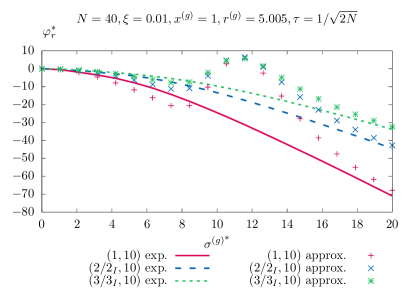
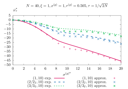
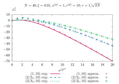
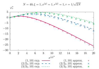
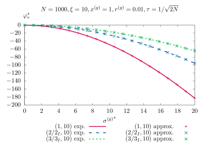
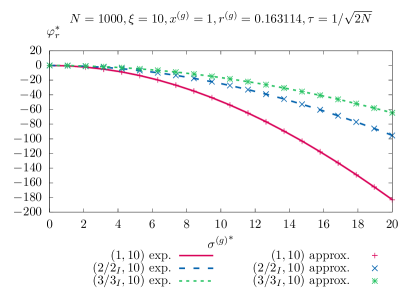
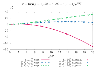
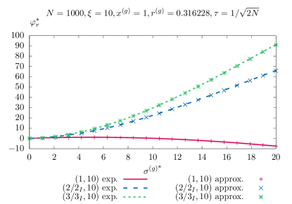
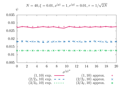
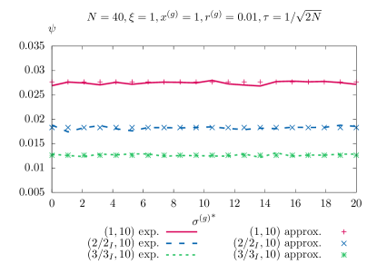
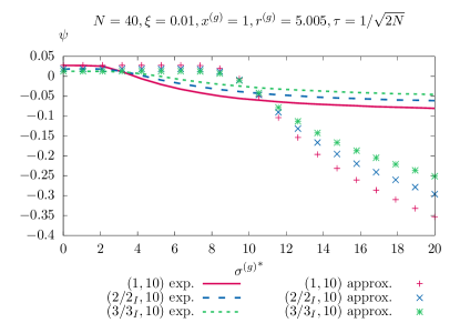
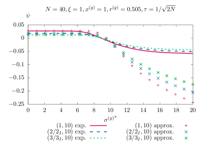
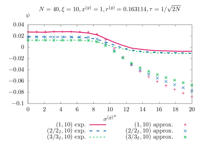
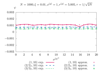
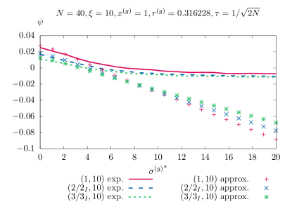
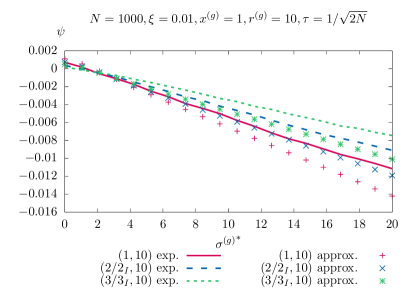
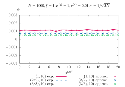
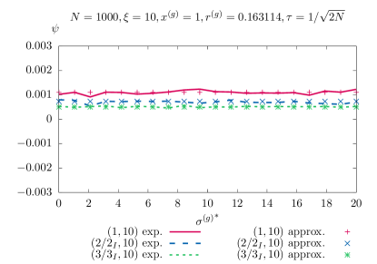
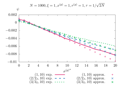
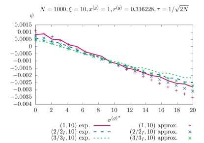
Figs. 10 to 18 show plots comparing the derived closed-form approximation for $\varphi_{x}^{*}$, $\varphi_{r}^{*}$, and $\psi$, respectively, with one-generation experiments. The pluses, crosses, and stars have been calculated by evaluating Equation 38 with Equations 15, 20, and 37, Equation 44 with Equations 15 and 37, and Equation 54 with Equation 15, respectively. The solid, dashed, and dotted lines have been generated by one-generation experiments. For this, the generational loop has been run $10^{5}$ times for a fixed parental individual and constant parameters. The experimentally determined values for $\varphi_{x}^{*}$, $\varphi_{r}^{*}$, and $\psi$ from those $10^{5}$ runs have been averaged. The top row in every set of $3\times 2$ plots shows the case that the parental individual is near the cone axis (note that here the feasible case dominates). The bottom row in every set of $3\times 2$ plots shows the case that the parental individual is in the vicinity of the cone boundary (note that here the infeasible case dominates). And the middle row shows a case in between.

Figure 10: Comparison of the $x$ progress rate approximation with simulations. (Part 1)

Figure 11: Comparison of the $x$ progress rate approximation with simulations. (Part 2)

Figure 12: Comparison of the $x$ progress rate approximation with simulations. (Part 3)

Figure 13: Comparison of the $r$ progress rate approximation with simulations. (Part 1)

Figure 14: Comparison of the $r$ progress rate approximation with simulations. (Part 2)

Figure 15: Comparison of the $r$ progress rate approximation with simulations. (Part 3)

Figure 16: Comparison of the SAR approximation with simulations. (Part 1)

Figure 17: Comparison of the SAR approximation with simulations. (Part 2)

Figure 18: Comparison of the SAR approximation with simulations. (Part 3)

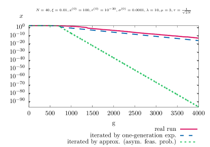
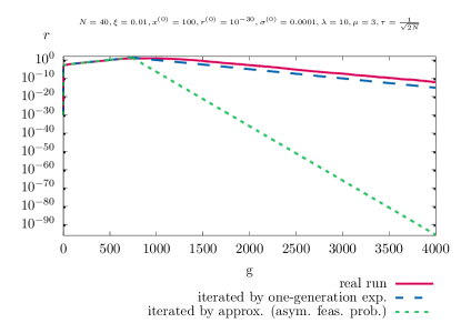
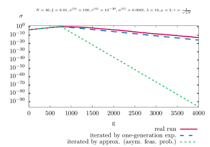
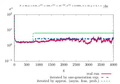
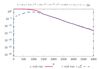
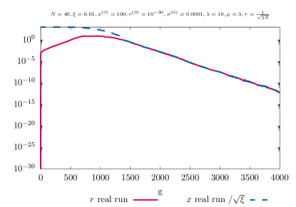
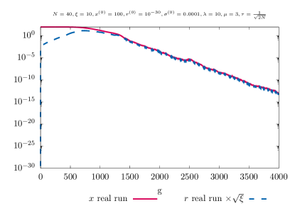
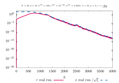
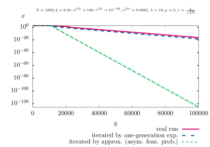
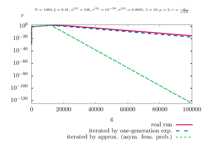
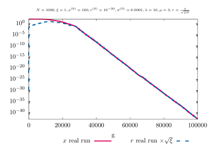
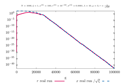
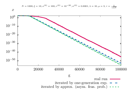
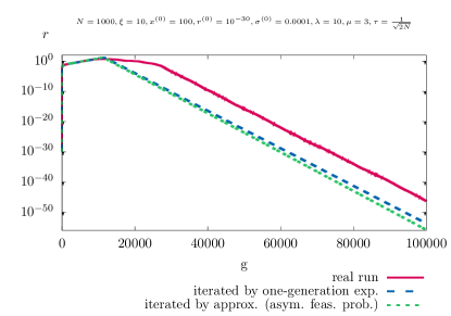
Figs. 19, 20, 21, 22, 23, and 24 show the mean value dynamics of the $(3/3_{I},10)$-ES applied to the conically constrained problem with different parameters as indicated in the title of the subplots. The plots are organized into three rows and two columns. The first two rows show the $x$ (first row, first column), $r$ (first row, second column), $\sigma$ (second row, first column), and $\sigma^{*}$ (second row, second column) dynamics. The third row shows $x$ and $r$ converted into each other by $\sqrt{\xi}$. The third row shows that after some initial phase, the ES transitions into a stationary state. In this steady state, the ES moves near the cone boundary. This becomes clear in the plots because the equation for the cone boundary is $r=x/\sqrt{\xi}$ or equivalently $x=r\sqrt{\xi}$. Furthermore, in this stationary state, the normalized mutation strength is constant on average. The lines for the real runs have been generated by averaging $100$ real runs of the ES. The lines for the iteration with one-generation experiments have been determined by iterating the mean value iterative system with one-generation experiments for ${\varphi^{(g)}_{x}}^{*}$, ${\varphi^{(g)}_{r}}^{*}$, and $\psi^{(g)}$. The lines for the iteration by approximation have been computed by iterating the mean value iterative system with the derived approximations in Section IV-B for ${\varphi^{(g)}_{x}}^{*}$, ${\varphi^{(g)}_{r}}^{*}$, and $\psi^{(g)}$. Note that due to the approximations used it is possible that in a generation $g$ the iteration of the mean value iterative system yields infeasible $(x^{(g)},r^{(g)})^{T}$. In such cases, the particular $(x^{(g)},r^{(g)})^{T}$ values have been projected back and projected values used in the further iterations.

Figure 19: Mean value dynamics closed-form approximation and real-run comparison of the $(3/3_{I},10)$-ES with repair by projection applied to the conically constrained problem. (Part 1)

Figure 20: Mean value dynamics closed-form approximation and real-run comparison of the $(3/3_{I},10)$-ES with repair by projection applied to the conically constrained problem. (Part 2)

Figure 21: Mean value dynamics closed-form approximation and real-run comparison of the $(3/3_{I},10)$-ES with repair by projection applied to the conically constrained problem. (Part 3)

Figure 22: Mean value dynamics closed-form approximation and real-run comparison of the $(3/3_{I},10)$-ES with repair by projection applied to the conically constrained problem. (Part 4)

Figure 23: Mean value dynamics closed-form approximation and real-run comparison of the $(3/3_{I},10)$-ES with repair by projection applied to the conically constrained problem. (Part 5)

Figure 24: Mean value dynamics closed-form approximation and real-run comparison of the $(3/3_{I},10)$-ES with repair by projection applied to the conically constrained problem. (Part 6)

IEEEtran app

References

- [1] D. V. Arnold, “On the behaviour of the (1, )-ES for a simple constrained problem,” in Proceedings of the 11th Workshop Proceedings on Foundations of Genetic Algorithms. ACM, 2011, pp. 15–24.
- [2] ——, “Analysis of a repair mechanism for the (1, )-ES applied to a simple constrained problem,” in Proceedings of the 13th Annual Conference on Genetic and Evolutionary Computation. ACM, 2011, pp. 853–860.
- [3] M. Hellwig and D. V. Arnold, “Comparison of constraint-handling mechanisms for the (1, )-ES on a simple constrained problem,” Evolutionary Computation, vol. 24, no. 1, pp. 1–23, 2016.
- [4] D. V. Arnold and J. Porter, “Towards an augmented lagrangian constraint handling approach for the (1+1)-ES,” in Proceedings of the 2015 Annual Conference on Genetic and Evolutionary Computation, ser. GECCO ’15. New York, NY, USA: ACM, 2015, pp. 249–256. [Online]. Available: http://doi.acm.org/10.1145/2739480.2754813
- [5] A. Atamna, A. Auger, and N. Hansen, “Augmented lagrangian constraint handling for CMA-ES - case of a single linear constraint,” in International Conference on Parallel Problem Solving from Nature. Springer, 2016, pp. 181–191.
- [6] ——, “Linearly convergent evolution strategies via augmented lagrangian constraint handling,” in Proceedings of the 14th ACM/SIGEVO Conference on Foundations of Genetic Algorithms. ACM, 2017, pp. 149–161.
- [7] D. V. Arnold, “On the behaviour of the (1, )-ES for a conically constrained problem,” in Proceedings of the 15th Annual Conference on Genetic and Evolutionary Computation. ACM, 2013, pp. 423–430.
- [8] P. Spettel and H.-G. Beyer, “Technical report: Analysis of the --self-adaptation evolution strategy with repair by projection applied to a conically constrained problem,” Vorarlberg University of Applied Sciences, Tech. Rep. TR-SAESCONE-18, 2018. [Online]. Available: https://www.fhv.at/fileadmin/user_upload/fhv/files/forschung/ppe/working-papers/Analysis_onecommalambdasigmaSA-ES_Projection_Cone_TR.pdf
- [9] H.-G. Beyer, The Theory of Evolution Strategies, ser. Natural Computing Series. Springer, 2001.
- [10] S. Meyer-Nieberg, “Self-adaptation in evolution strategies,” Ph.D. dissertation, Dortmund University of Technology, 12 2007.