Bifurcations in the RG-Flow of QCD

Folkert Kuipers1,    Umut Gürsoy1    and Yuri Kuznetsov2
1Institute for Theoretical Physics, Utrecht University, 3584 CC Utrecht, The Netherlands
2Mathematical Institute, Utrecht University, 3584 CC Utrecht, The Netherlands
E-mail: F.Kuipers@sussex.ac.ukE-mail: U.Gursoy@uu.nlE-mail: I.A.Kouzenetsov@uu.nl
Abstract

Bifurcation analysis is used to study an effective model of QCD4 with four-fermi interactions. Our analysis supports the scenario of a fixed point merger at the lower edge of the conformal window. This indicates square root scaling of the anomalous scaling dimensions of the fermion fields just above the lower edge and exponential scaling just below. We also predict existence of new fixed points in this model whose (dis)appearance may indicate transitions of the flow within the conformal window. Furthermore, we make new predictions for the critical value (Nf/Nc)critsubscriptsubscript𝑁𝑓subscript𝑁𝑐crit(N_{f}/N_{c})_{\textrm{crit}} at the lower edge. We also obtain exotic spiraling flows that are generated by complex scaling dimensions of the effective four-fermi interactions. Finally, we extend the model by adding a scalar field that couples with a Yukawa interaction term and study the modifications it causes to RG-flows.

1 Introduction

Renormalization group describes the flow of a theory in the space spanned by the coupling constants called the “theory space”. In quantum field theory renormalization group flows are governed by a set of beta functions that result in ordinary differential equations. The flow induced by these beta functions provide information about the change of coupling constants and anomalous field dimensions with the energy scale. An interesting aspect of the RG flows are the fixed points where the beta functions vanish. In particular one is interested in determining the positions of these fixed points and their stability properties. In addition one would like to obtain possible renormalized trajectories generated by the beta functions. Since the RG flows are generated by ordinary differential equations, it is natural to study them with the tools developed for the theory of dynamical systems. In this article, we use analytical and numerical111Throughout the article we make extensive use of the MATLAB package MatCont [1, 2] methods for bifurcation analysis to study bifurcations in renormalization group flows, as recently proposed by Gukov [3].

Bifurcation theory, which we summarize in Appendix A, categorizes topological changes in a dynamical system and is therefore an ideal tool to study the appearance and disappearance of fixed points. Using this categorization, we can not only determine easily when fixed points appear and disappear on the RG flow, but also obtain information about the nature of these transitions where the fixed points (dis)appear. As discussed in [4], there are three typical ways in which fixed points of an RG-flow (dis)appear:

  • Merger of a fixed point with non-trivial coupling constant and a fixed point with a trivial coupling constant. At this merger the stability of the non-trivial fixed point changes.

  • Merger of two fixed point with non-trivial coupling constants. At this merger both fixed points disappear.

  • A divergent fixed-point as one or multiple coupling constants run off to infinity.

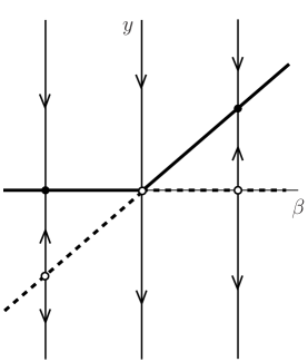
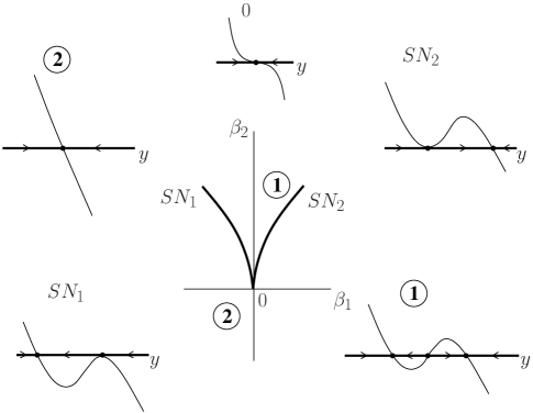
The first and the second scenarios are examples of standard bifurcations. The second is naturally described by the well known saddle-node bifurcation, while the first is called a transcritical bifurcation. It should be noted that in this scenario the fixed points usually do not merge as was stated in [4] but collide and exchange stability. However, at this transition the coupling constant at the non-trivial fixed point generally becomes negative, hence moves into a physical uninteresting region. Furthermore, it is an easy exercise to show that the first scenario always induces a linear scaling of the anomalous dimension at the fixed point [3], while the second scenario implies square root [3] and exponential (also known as BKT or Miransky scaling) scaling of the anomalous dimensions [4] at the two sides of the merger. Finally, the third scenario above with diverging fixed points is much harder to describe using the techniques from the bifurcation theory. However, this scenario is mostly encountered in a perturbative analysis of the RG flows which becomes invalid anyway at the divergence. It turns out that in some cases this last scenario is replaced by the second one in an effective field theory.

In this paper, we apply bifurcation analysis to an effective model of QCD as suggested in [3]. We consider QCD4 with gauge group SU(Nc)𝑆𝑈subscript𝑁𝑐SU(N_{c}) with an arbitrary number of colors Ncsubscript𝑁𝑐N_{c} and flavors, Nfsubscript𝑁𝑓N_{f}, as the bifurcation parameters. The Lagrangian is given by

=14GμνAGAμν+i=1Nfψ¯ai(ibamiδba)ψbi,14superscriptsubscript𝐺𝜇𝜈𝐴subscriptsuperscript𝐺𝜇𝜈𝐴superscriptsubscript𝑖1subscript𝑁𝑓subscript¯𝜓𝑎𝑖𝑖superscriptsubscriptitalic-D̸𝑏𝑎subscript𝑚𝑖superscriptsubscript𝛿𝑏𝑎superscript𝜓𝑏𝑖\mathcal{L}=-\frac{1}{4}G_{\mu\nu}^{A}G^{\mu\nu}_{A}+\sum_{i=1}^{N_{f}}\bar{\psi}_{ai}\left(i\not{D}_{b}^{a}-m_{i}\delta_{b}^{a}\right)\psi^{bi}\,, (1)

where GAsubscript𝐺𝐴G_{A} are the gluon field strengths and ψisubscript𝜓𝑖\psi_{i} are the fermions of flavor i𝑖i. Furthermore a,b,c𝑎𝑏𝑐a,b,c are used to label the color in the fundamental representation, and A,B,C𝐴𝐵𝐶A,B,C is used for the color in the adjoint representation. We have

GμνA=μAνAνAμA+gfABCAμBAνCand=γμ(μigtAAμA).formulae-sequencesuperscriptsubscript𝐺𝜇𝜈𝐴subscript𝜇superscriptsubscript𝐴𝜈𝐴subscript𝜈superscriptsubscript𝐴𝜇𝐴𝑔superscript𝑓𝐴𝐵𝐶superscriptsubscript𝐴𝜇𝐵superscriptsubscript𝐴𝜈𝐶anditalic-D̸superscript𝛾𝜇subscript𝜇𝑖𝑔subscript𝑡𝐴superscriptsubscript𝐴𝜇𝐴G_{\mu\nu}^{A}=\partial_{\mu}A_{\nu}^{A}-\partial_{\nu}A_{\mu}^{A}+gf^{ABC}A_{\mu}^{B}A_{\nu}^{C}\quad\textrm{and}\quad\not{D}=\gamma^{\mu}\left(\partial_{\mu}-igt_{A}A_{\mu}^{A}\right).

We will consider the massless case, mi=0isubscript𝑚𝑖0for-all𝑖m_{i}=0\;\forall i, where the Lagrangian becomes invariant under a global SU(Nf)L×SU(Nf)R×U(1)𝑆𝑈subscriptsubscript𝑁𝑓𝐿𝑆𝑈subscriptsubscript𝑁𝑓𝑅𝑈1SU(N_{f})_{L}\times SU(N_{f})_{R}\times U(1) symmetry which can be broken to SU(Nf)V𝑆𝑈subscriptsubscript𝑁𝑓𝑉SU(N_{f})_{V} by formation of a chiral condensate.

The two-loop beta function for the gauge coupling is given by [5]

βg[2]ΛdαgdΛ=2b0αg22b1αg3superscriptsubscript𝛽𝑔delimited-[]2Λ𝑑subscript𝛼𝑔𝑑Λ2subscript𝑏0superscriptsubscript𝛼𝑔22subscript𝑏1superscriptsubscript𝛼𝑔3\beta_{g}^{[2]}\equiv\Lambda\frac{d\alpha_{g}}{d\Lambda}=-2b_{0}\alpha_{g}^{2}-2b_{1}\alpha_{g}^{3} (2)

with αg:=g2(4π)2assignsubscript𝛼𝑔superscript𝑔2superscript4𝜋2\alpha_{g}:=\frac{g^{2}}{(4\pi)^{2}} and

b0subscript𝑏0\displaystyle b_{0} =113Nc23Nf,absent113subscript𝑁𝑐23subscript𝑁𝑓\displaystyle=\frac{11}{3}N_{c}-\frac{2}{3}N_{f}, (3)
b1subscript𝑏1\displaystyle b_{1} =343Nc2Nf(Nc21Nc+103Nc),absent343superscriptsubscript𝑁𝑐2subscript𝑁𝑓superscriptsubscript𝑁𝑐21subscript𝑁𝑐103subscript𝑁𝑐\displaystyle=\frac{34}{3}N_{c}^{2}-N_{f}\left(\frac{N_{c}^{2}-1}{N_{c}}+\frac{10}{3}N_{c}\right), (4)

are the scheme independent beta-function coefficients. This beta function has a (degenerate) trivial root at αg=0subscript𝛼𝑔0\alpha_{g}=0, and a non-trivial root at αg=b0b1subscript𝛼𝑔subscript𝑏0subscript𝑏1\alpha_{g}=-\frac{b_{0}}{b_{1}}. The non-trivial fixed point becomes negative and therefore unphysical for

xNfNc>112,𝑥subscript𝑁𝑓subscript𝑁𝑐112\displaystyle x\equiv\frac{N_{f}}{N_{c}}>\frac{11}{2}\,, (5)

and

NfNc<34Nc213Nc23,subscript𝑁𝑓subscript𝑁𝑐34superscriptsubscript𝑁𝑐213superscriptsubscript𝑁𝑐23\frac{N_{f}}{N_{c}}<\frac{34N_{c}^{2}}{13N_{c}^{2}-3}\,, (6)

where the latter bound runs between 3.4 and 2.6 for 1<Nc<1subscript𝑁𝑐1<N_{c}<\infty, thus it is always below the first bound for any Ncsubscript𝑁𝑐N_{c}. The region between these bounds, where a non-trivial fixed point exists, is known as the conformal window (cf. figure 1), and its existence was first discussed in [5, 6]. Within the conformal window the non-trivial fixed point is attractive in the IR limit, while the trivial fixed point is attractive in the UV. Above the conformal window, the trivial fixed point becomes an IR attractor. Since αgntsuperscriptsubscript𝛼𝑔𝑛𝑡\alpha_{g}^{nt} becomes small close to x=11/2𝑥112x=11/2 higher order contributions to the beta function (2) can be neglected hence the value of upper bound is robust. However, close to the lower edge αgsubscript𝛼𝑔\alpha_{g} becomes very large, invalidates the above estimate and (6) becomes unreliable. In particular, other fixed points resulting from higher order terms might influence this critical value.

The type of phase transition that occurs at the lower edge of the conformal window, that we call xcritsubscript𝑥𝑐𝑟𝑖𝑡x_{crit}, and its value has been a central problem in the literature. Use of Schwinger-Dyson equations [17, 22, 21, 19] generically suggest that the theory is in the confining phase with chiral symmetry breaking for x𝑥x below xcritsubscript𝑥𝑐𝑟𝑖𝑡x_{crit}, see figure 1. As for the value of xcritsubscript𝑥𝑐𝑟𝑖𝑡x_{crit}, estimates for Nc=3subscript𝑁𝑐3N_{c}=3 are typically in the range 6xcrit12less-than-or-approximately-equals6subscript𝑥critless-than-or-approximately-equals126\lessapprox x_{\textrm{crit}}\lessapprox 12 [7, 8, 9, 10, 11, 12, 13, 14, 15, 16, 17, 18, 19, 20, 21, 22, 23], and follow from the various techniques (cf. Table 6 of [3] for a recent overview of various studies and their prediction). A more recent study [24, 25] uses Potts models to discuss the behaviour at the lower edge of the conformal window. The transition at the lower edge could be first order [26, 27] or infinite order [4, 22], and can be analyzed through several methods. This is an important open problem as characterization of this phase transition will lead to a better understanding of the strong interactions and might be relevant for model building beyond the standard model [27]. Furthermore, functional RG and holographic approaches indicate that the conformal window is continuously connected to the quark gluon plasma phase at finite temperature [28, 29, 30]. Therefore studies of the conformal window may provide crucial information on the quark gluon plasma and vice versa.

Several works in the literature [9, 27, 28, 24, 25] point toward the possibility that the IR stable fixed point αg=b0/b1subscript𝛼𝑔subscript𝑏0subscript𝑏1\alpha_{g}=-b_{0}/b_{1} annihilates with another fixed point of the RG flow at xcritsubscript𝑥𝑐𝑟𝑖𝑡x_{crit} in the form of a saddle-node bifurcation (second option in the list above). This would in turn indicate that a UV irrelevant operator, such as a 4-fermi interaction, crosses marginality precisely at xcritsubscript𝑥𝑐𝑟𝑖𝑡x_{crit} [3] as already anticipated in the early literature [21, 20, 23]. In this paper, we investigate this possibility by considering an effective model for QCD4 that includes four-fermi interactions and determine all fixed points within this model in and around the conformal window. Furthermore, we discuss how they appear and disappear as the bifurcation parameters Ncsubscript𝑁𝑐N_{c} and Nfsubscript𝑁𝑓N_{f} are varied. Finally we study the effects of adding a scalar operator with a Yukawa type interaction to our results in this effective theory.

Refer to caption
Figure 1: Phase diagram of QCD as a function of x=Nf/Nc𝑥subscript𝑁𝑓subscript𝑁𝑐x=N_{f}/N_{c} at zero temperature and zero chemical potential.

The paper is organized as follows. In the next section we introduce the effective model with the four-fermi interactions, derive the beta function equations both for finite values of Ncsubscript𝑁𝑐N_{c} and Nfsubscript𝑁𝑓N_{f} and in the Veneziano limit, and study the fixed point structure using bifurcation theory in detail. In section 4, we extend the model including the scalar operator. We conclude and discuss our results and list possible future work in the last section. Appendix A provides a short introduction to bifurcation theory in dynamical systems and Appendix B details the calculation of the beta-functions in perturbation theory.

2 An effective model for QCD

2.1 Beta functions in an effective model for QCD

We study the theory in the Wilsonian picture. For this, we write down the effective action, which is given by the Legendre transform of the Lagrangian (1) with mi=0subscript𝑚𝑖0m_{i}=0. We impose the symmetries obeyed by the Lagrangian on the effective action and expand the effective action in the quark fields ψaisuperscript𝜓𝑎𝑖\psi^{ai} up to the 4-quark interactions, as was done in [15]. This yields

ΓΛ=d4x(14g2GμνAGAμν+ψ¯aiiψai+4f),subscriptΓΛsuperscript𝑑4𝑥14superscript𝑔2superscriptsubscript𝐺𝜇𝜈𝐴superscriptsubscript𝐺𝐴𝜇𝜈subscript¯𝜓𝑎𝑖𝑖italic-D̸superscript𝜓𝑎𝑖subscript4𝑓\Gamma_{\Lambda}=\int d^{4}x\left(-\frac{1}{4g^{2}}G_{\mu\nu}^{A}G_{A}^{\mu\nu}+\bar{\psi}_{ai}i\not{D}\psi^{ai}+\mathcal{L}_{4f}\right), (7)

where 4fsubscript4𝑓\mathcal{L}_{4f} denote the four-fermi interactions and we redefined the gauge fields

AA=gA𝐴superscript𝐴𝑔𝐴A\rightarrow A^{\prime}=gA (8)

such that

GμνA1gGμνAandDμ=μitAAμA.formulae-sequencesuperscriptsubscript𝐺𝜇𝜈𝐴1𝑔superscriptsubscript𝐺𝜇𝜈𝐴andsubscript𝐷𝜇subscript𝜇𝑖subscript𝑡𝐴subscriptsuperscript𝐴𝐴𝜇G_{\mu\nu}^{A}\rightarrow\frac{1}{g}G_{\mu\nu}^{A}\quad\textrm{and}\quad D_{\mu}=\partial_{\mu}-it_{A}A^{\prime A}_{\mu}. (9)

One can write down four independent four-fermi operators [31, 32, 33, 34] respecting the symmetries. We choose a basis as in [34, 15]:

4f=GSΛ2(1+η)𝒪S+GVΛ2(1+η)𝒪V+GV1Λ2(1+η)𝒪V1+GV2Λ2(1+η)𝒪V2,subscript4𝑓subscript𝐺𝑆superscriptΛ21𝜂subscript𝒪𝑆subscript𝐺𝑉superscriptΛ21𝜂subscript𝒪𝑉subscript𝐺subscript𝑉1superscriptΛ21𝜂subscript𝒪subscript𝑉1subscript𝐺subscript𝑉2superscriptΛ21𝜂subscript𝒪subscript𝑉2\mathcal{L}_{4f}=\frac{G_{S}}{\Lambda^{2(1+\eta)}}\mathcal{O}_{S}+\frac{G_{V}}{\Lambda^{2(1+\eta)}}\mathcal{O}_{V}+\frac{G_{V_{1}}}{\Lambda^{2(1+\eta)}}\mathcal{O}_{V_{1}}+\frac{G_{V_{2}}}{\Lambda^{2(1+\eta)}}\mathcal{O}_{V_{2}},

where η=γψ𝜂subscript𝛾𝜓\eta=\gamma_{\psi} is the anomalous dimension of the fermion field and

𝒪Ssubscript𝒪𝑆\displaystyle\mathcal{O}_{S} =2L¯iRjR¯jLi=12[ψ¯iψjψ¯jψiψ¯iγ5ψjψ¯jγ5ψi],absent2subscript¯𝐿𝑖superscript𝑅𝑗subscript¯𝑅𝑗superscript𝐿𝑖12delimited-[]subscript¯𝜓𝑖superscript𝜓𝑗subscript¯𝜓𝑗superscript𝜓𝑖subscript¯𝜓𝑖subscript𝛾5superscript𝜓𝑗subscript¯𝜓𝑗subscript𝛾5superscript𝜓𝑖\displaystyle=2\bar{L}_{i}R^{j}\bar{R}_{j}L^{i}=\frac{1}{2}[\bar{\psi}_{i}\psi^{j}\bar{\psi}_{j}\psi^{i}-\bar{\psi}_{i}\gamma_{5}\psi^{j}\bar{\psi}_{j}\gamma_{5}\psi^{i}],
𝒪Vsubscript𝒪𝑉\displaystyle\mathcal{O}_{V} =L¯iγμLjL¯jγμLi+(LR)=12[ψ¯iγμψjψ¯jγμψi+ψ¯iγμγ5ψjψ¯jγμγ5ψi],\displaystyle=\bar{L}_{i}\gamma^{\mu}L^{j}\bar{L}_{j}\gamma_{\mu}L^{i}+(L\leftrightarrow R)=\frac{1}{2}[\bar{\psi}_{i}\gamma^{\mu}\psi^{j}\bar{\psi}_{j}\gamma_{\mu}\psi^{i}+\bar{\psi}_{i}\gamma^{\mu}\gamma_{5}\psi^{j}\bar{\psi}_{j}\gamma_{\mu}\gamma_{5}\psi^{i}],
𝒪V1subscript𝒪subscript𝑉1\displaystyle\mathcal{O}_{V_{1}} =2L¯iγμLiR¯jγμRj=12[(ψ¯iγμψi)2(ψ¯iγμγ5ψi)2],absent2subscript¯𝐿𝑖superscript𝛾𝜇superscript𝐿𝑖subscript¯𝑅𝑗subscript𝛾𝜇superscript𝑅𝑗12delimited-[]superscriptsubscript¯𝜓𝑖superscript𝛾𝜇superscript𝜓𝑖2superscriptsubscript¯𝜓𝑖superscript𝛾𝜇subscript𝛾5superscript𝜓𝑖2\displaystyle=2\bar{L}_{i}\gamma^{\mu}L^{i}\bar{R}_{j}\gamma_{\mu}R^{j}=\frac{1}{2}[(\bar{\psi}_{i}\gamma^{\mu}\psi^{i})^{2}-(\bar{\psi}_{i}\gamma^{\mu}\gamma_{5}\psi^{i})^{2}],
𝒪V2subscript𝒪subscript𝑉2\displaystyle\mathcal{O}_{V_{2}} =(L¯iγμLi)2+(LR)=12[(ψ¯iγμψi)2+(ψ¯iγμγ5ψi)2]\displaystyle=(\bar{L}_{i}\gamma^{\mu}L^{i})^{2}+(L\leftrightarrow R)=\frac{1}{2}[(\bar{\psi}_{i}\gamma^{\mu}\psi^{i})^{2}+(\bar{\psi}_{i}\gamma^{\mu}\gamma_{5}\psi^{i})^{2}]

One can calculate the beta functions of the four-fermi interactions using the Wetterich equation given in Appendix B.3. The beta function for the gauge coupling αgsubscript𝛼𝑔\alpha_{g} cannot be derived from the effective action (7) easily as one needs an expansion in the gluon fields in the effective action [15] which complicates the calculation substantially. Instead, we can start from the perturbative equation (2) and add the effective four-fermi interactions to it. We provide this calculation in appendix B.2 and obtain the same result as in [15]. The complete set of beta-functions is then given by222We find slightly different beta functions for the four-fermi interactions from the ones presented in [15]. They agree in the Veneziano limit however.

{ΛdαgdΛ=23(11Nc2Nf)αg223(34Nc213NcNf+3NfNc)αg3+2NcNfgVαg2,ΛdgSdΛ=2gS2NcgS2+2NfgSgV+6gSgV1+2gSgV26(Nc1Nc)gSαg+12gV1αg32(3Nc8Nc)αg2,ΛdgVdΛ=2gV+Nf4gS2+(Nc+Nf)gV26gVgV26NcgV+6gV2αg34(Nc8Nc)αg2,ΛdgV1dΛ=2gV114gS2gSgV3gV12NfgSgV2+2(Nc+Nf)gVgV1+2(NcNf+1)gV1gV2+6NcgV1αg+34(1+4Nc2)αg2,ΛdgV2dΛ=2gV23gV2NcNfgV12+(NcNf2)gV22NfgSgV1+2(Nc+Nf)gVgV2+6gVαg6NcgV2αg34(3+4Nc2)αg2,casesΛ𝑑subscript𝛼𝑔𝑑Λabsent2311subscript𝑁𝑐2subscript𝑁𝑓superscriptsubscript𝛼𝑔22334superscriptsubscript𝑁𝑐213subscript𝑁𝑐subscript𝑁𝑓3subscript𝑁𝑓subscript𝑁𝑐superscriptsubscript𝛼𝑔32subscript𝑁𝑐subscript𝑁𝑓subscript𝑔𝑉superscriptsubscript𝛼𝑔2Λ𝑑subscript𝑔𝑆𝑑Λabsent2subscript𝑔𝑆2subscript𝑁𝑐superscriptsubscript𝑔𝑆22subscript𝑁𝑓subscript𝑔𝑆subscript𝑔𝑉6subscript𝑔𝑆subscript𝑔subscript𝑉12subscript𝑔𝑆subscript𝑔subscript𝑉2otherwise6subscript𝑁𝑐1subscript𝑁𝑐subscript𝑔𝑆subscript𝛼𝑔12subscript𝑔subscript𝑉1subscript𝛼𝑔323subscript𝑁𝑐8subscript𝑁𝑐superscriptsubscript𝛼𝑔2Λ𝑑subscript𝑔𝑉𝑑Λabsent2subscript𝑔𝑉subscript𝑁𝑓4superscriptsubscript𝑔𝑆2subscript𝑁𝑐subscript𝑁𝑓superscriptsubscript𝑔𝑉26subscript𝑔𝑉subscript𝑔subscript𝑉2otherwise6subscript𝑁𝑐subscript𝑔𝑉6subscript𝑔subscript𝑉2subscript𝛼𝑔34subscript𝑁𝑐8subscript𝑁𝑐superscriptsubscript𝛼𝑔2Λ𝑑subscript𝑔subscript𝑉1𝑑Λabsent2subscript𝑔subscript𝑉114superscriptsubscript𝑔𝑆2subscript𝑔𝑆subscript𝑔𝑉3superscriptsubscript𝑔subscript𝑉12subscript𝑁𝑓subscript𝑔𝑆subscript𝑔subscript𝑉22subscript𝑁𝑐subscript𝑁𝑓subscript𝑔𝑉subscript𝑔subscript𝑉1otherwise2subscript𝑁𝑐subscript𝑁𝑓1subscript𝑔subscript𝑉1subscript𝑔subscript𝑉26subscript𝑁𝑐subscript𝑔subscript𝑉1subscript𝛼𝑔3414superscriptsubscript𝑁𝑐2superscriptsubscript𝛼𝑔2Λ𝑑subscript𝑔subscript𝑉2𝑑Λabsent2subscript𝑔subscript𝑉23superscriptsubscript𝑔𝑉2subscript𝑁𝑐subscript𝑁𝑓superscriptsubscript𝑔subscript𝑉12subscript𝑁𝑐subscript𝑁𝑓2superscriptsubscript𝑔subscript𝑉22subscript𝑁𝑓subscript𝑔𝑆subscript𝑔subscript𝑉1otherwise2subscript𝑁𝑐subscript𝑁𝑓subscript𝑔𝑉subscript𝑔subscript𝑉26subscript𝑔𝑉subscript𝛼𝑔6subscript𝑁𝑐subscript𝑔subscript𝑉2subscript𝛼𝑔3434superscriptsubscript𝑁𝑐2superscriptsubscript𝛼𝑔2\begin{cases}\Lambda\frac{d\alpha_{g}}{d\Lambda}=&-\frac{2}{3}(11N_{c}-2N_{f})\alpha_{g}^{2}-\frac{2}{3}\left(34N_{c}^{2}-13N_{c}N_{f}+3\frac{N_{f}}{N_{c}}\right)\alpha_{g}^{3}+2N_{c}N_{f}g_{V}\alpha_{g}^{2},\\ \Lambda\frac{dg_{S}}{d\Lambda}=&2g_{S}-2N_{c}g_{S}^{2}+2N_{f}g_{S}g_{V}+6g_{S}g_{V_{1}}+2g_{S}g_{V_{2}}\\ &-6\left(N_{c}-\frac{1}{N_{c}}\right)g_{S}\alpha_{g}+12g_{V_{1}}\alpha_{g}-\frac{3}{2}\left(3N_{c}-\frac{8}{N_{c}}\right)\alpha_{g}^{2},\\ \Lambda\frac{dg_{V}}{d\Lambda}=&2g_{V}+\frac{N_{f}}{4}g_{S}^{2}+(N_{c}+N_{f})g_{V}^{2}-6g_{V}g_{V_{2}}\\ &-\frac{6}{N_{c}}g_{V}+6g_{V_{2}}\alpha_{g}-\frac{3}{4}\left(N_{c}-\frac{8}{N_{c}}\right)\alpha_{g}^{2},\\ \Lambda\frac{dg_{V_{1}}}{d\Lambda}=&2g_{V_{1}}-\frac{1}{4}g_{S}^{2}-g_{S}g_{V}-3g_{V_{1}}^{2}-N_{f}g_{S}g_{V_{2}}+2(N_{c}+N_{f})g_{V}g_{V_{1}}\\ &+2(N_{c}N_{f}+1)g_{V_{1}}g_{V_{2}}+\frac{6}{N_{c}}g_{V_{1}}\alpha_{g}+\frac{3}{4}\left(1+\frac{4}{N_{c}^{2}}\right)\alpha_{g}^{2},\\ \Lambda\frac{dg_{V_{2}}}{d\Lambda}=&2g_{V_{2}}-3g_{V}^{2}-N_{c}N_{f}g_{V_{1}}^{2}+(N_{c}N_{f}-2)g_{V_{2}}^{2}-N_{f}g_{S}g_{V_{1}}\\ &+2(N_{c}+N_{f})g_{V}g_{V_{2}}+6g_{V}\alpha_{g}-\frac{6}{N_{c}}g_{V_{2}}\alpha_{g}-\frac{3}{4}\left(3+\frac{4}{N_{c}^{2}}\right)\alpha_{g}^{2},\end{cases} (10)

where we defined the rescaled variables

αg:=g2(4π)2,gi:=Gi4π2.formulae-sequenceassignsubscript𝛼𝑔superscript𝑔2superscript4𝜋2assignsubscript𝑔𝑖subscript𝐺𝑖4superscript𝜋2\alpha_{g}:=\frac{g^{2}}{(4\pi)^{2}},\quad g_{i}:=\frac{G_{i}}{4\pi^{2}}. (11)

Let us further define

x:=NfNc,N:=Nc,formulae-sequenceassign𝑥subscript𝑁𝑓subscript𝑁𝑐assign𝑁subscript𝑁𝑐x:=\frac{N_{f}}{N_{c}},\quad N:=N_{c},

and perform the rescaling

Nαg𝑁subscript𝛼𝑔\displaystyle N\alpha_{g} αgabsentsubscript𝛼𝑔\displaystyle\rightarrow\alpha_{g}
NgS𝑁subscript𝑔𝑆\displaystyle Ng_{S} gSabsentsubscript𝑔𝑆\displaystyle\rightarrow g_{S}
NgV𝑁subscript𝑔𝑉\displaystyle Ng_{V} gVabsentsubscript𝑔𝑉\displaystyle\rightarrow g_{V} (12)
N2gV1superscript𝑁2subscript𝑔subscript𝑉1\displaystyle N^{2}g_{V_{1}} gV1absentsubscript𝑔subscript𝑉1\displaystyle\rightarrow g_{V_{1}}
N2gV2superscript𝑁2subscript𝑔subscript𝑉2\displaystyle N^{2}g_{V_{2}} gV2,absentsubscript𝑔subscript𝑉2\displaystyle\rightarrow g_{V_{2}},

which makes the set (10) amenable to the Veneziano limit where N𝑁N\rightarrow\infty and x𝑥x remains finite. After the rescaling we obtain

{ΛdαgdΛ=23(112x)αg223(3413x)αg3+2xgVαg2+N2(2xαg3),ΛdgSdΛ=2gS2gS2+2xgSgV6gSαg92αg2+N2(6gSgV1+2gSgV2+6gSαg+12gV1αg+12αg2),ΛdgVdΛ=2gV+14xgS2+(1+x)gV234αg2+N2(6gVgV26gVαg+6gV2αg+6αg2),ΛdgV1dΛ=2gV114gs2gSgVxgSgV2+2(1+x)gVgV1+2xgV1gV2+34αg2+N2(3gV12+2gV1gV2+6gV1αg+3αg2),ΛdgV2dΛ=2gV23gV2xgV12+xgV22xgSgV1+2(1+x)gVgV2+6gVαg94αg2+N2(2gV226gV2αg3αg2).casesΛ𝑑subscript𝛼𝑔𝑑Λabsent23112𝑥superscriptsubscript𝛼𝑔2233413𝑥superscriptsubscript𝛼𝑔32𝑥subscript𝑔𝑉superscriptsubscript𝛼𝑔2otherwisesuperscript𝑁22𝑥superscriptsubscript𝛼𝑔3Λ𝑑subscript𝑔𝑆𝑑Λabsent2subscript𝑔𝑆2superscriptsubscript𝑔𝑆22𝑥subscript𝑔𝑆subscript𝑔𝑉6subscript𝑔𝑆subscript𝛼𝑔92superscriptsubscript𝛼𝑔2otherwisesuperscript𝑁26subscript𝑔𝑆subscript𝑔subscript𝑉12subscript𝑔𝑆subscript𝑔subscript𝑉26subscript𝑔𝑆subscript𝛼𝑔12subscript𝑔subscript𝑉1subscript𝛼𝑔12superscriptsubscript𝛼𝑔2Λ𝑑subscript𝑔𝑉𝑑Λabsent2subscript𝑔𝑉14𝑥superscriptsubscript𝑔𝑆21𝑥superscriptsubscript𝑔𝑉234superscriptsubscript𝛼𝑔2otherwisesuperscript𝑁26subscript𝑔𝑉subscript𝑔subscript𝑉26subscript𝑔𝑉subscript𝛼𝑔6subscript𝑔subscript𝑉2subscript𝛼𝑔6superscriptsubscript𝛼𝑔2Λ𝑑subscript𝑔subscript𝑉1𝑑Λabsent2subscript𝑔subscript𝑉114superscriptsubscript𝑔𝑠2subscript𝑔𝑆subscript𝑔𝑉𝑥subscript𝑔𝑆subscript𝑔subscript𝑉221𝑥subscript𝑔𝑉subscript𝑔subscript𝑉12𝑥subscript𝑔subscript𝑉1subscript𝑔subscript𝑉234superscriptsubscript𝛼𝑔2otherwisesuperscript𝑁23superscriptsubscript𝑔subscript𝑉122subscript𝑔subscript𝑉1subscript𝑔subscript𝑉26subscript𝑔subscript𝑉1subscript𝛼𝑔3superscriptsubscript𝛼𝑔2Λ𝑑subscript𝑔subscript𝑉2𝑑Λabsent2subscript𝑔subscript𝑉23superscriptsubscript𝑔𝑉2𝑥superscriptsubscript𝑔subscript𝑉12𝑥superscriptsubscript𝑔subscript𝑉22𝑥subscript𝑔𝑆subscript𝑔subscript𝑉121𝑥subscript𝑔𝑉subscript𝑔subscript𝑉26subscript𝑔𝑉subscript𝛼𝑔94superscriptsubscript𝛼𝑔2otherwisesuperscript𝑁22superscriptsubscript𝑔subscript𝑉226subscript𝑔subscript𝑉2subscript𝛼𝑔3superscriptsubscript𝛼𝑔2\begin{cases}\Lambda\frac{d\alpha_{g}}{d\Lambda}=&-\frac{2}{3}(11-2x)\alpha_{g}^{2}-\frac{2}{3}(34-13x)\alpha_{g}^{3}+2xg_{V}\alpha_{g}^{2}\\ &+N^{-2}\left(-2x\alpha_{g}^{3}\right),\\ \Lambda\frac{dg_{S}}{d\Lambda}=&2g_{S}-2g_{S}^{2}+2xg_{S}g_{V}-6g_{S}\alpha_{g}-\frac{9}{2}\alpha_{g}^{2}\\ &+N^{-2}\left(6g_{S}g_{V_{1}}+2g_{S}g_{V_{2}}+6g_{S}\alpha_{g}+12g_{V_{1}}\alpha_{g}+12\alpha_{g}^{2}\right),\\ \Lambda\frac{dg_{V}}{d\Lambda}=&2g_{V}+\frac{1}{4}xg_{S}^{2}+(1+x)g_{V}^{2}-\frac{3}{4}\alpha_{g}^{2}\\ &+N^{-2}\left(-6g_{V}g_{V_{2}}-6g_{V}\alpha_{g}+6g_{V_{2}}\alpha_{g}+6\alpha_{g}^{2}\right),\\ \Lambda\frac{dg_{V_{1}}}{d\Lambda}=&2g_{V_{1}}-\frac{1}{4}g_{s}^{2}-g_{S}g_{V}-xg_{S}g_{V_{2}}+2(1+x)g_{V}g_{V_{1}}+2xg_{V_{1}}g_{V_{2}}+\frac{3}{4}\alpha_{g}^{2}\\ &+N^{-2}\left(-3g_{V_{1}}^{2}+2g_{V_{1}}g_{V_{2}}+6g_{V_{1}}\alpha_{g}+3\alpha_{g}^{2}\right),\\ \Lambda\frac{dg_{V_{2}}}{d\Lambda}=&2g_{V_{2}}-3g_{V}^{2}-xg_{V_{1}}^{2}+xg_{V_{2}}^{2}-xg_{S}g_{V_{1}}+2(1+x)g_{V}g_{V_{2}}+6g_{V}\alpha_{g}-\frac{9}{4}\alpha_{g}^{2}\\ &+N^{-2}\left(-2g_{V_{2}}^{2}-6g_{V_{2}}\alpha_{g}-3\alpha_{g}^{2}\right).\end{cases} (13)

2.2 Veneziano Limit

In this section, we study the Veneziano limit of the model (13) as was done in [3] and [15]. The Veneziano limit, N𝑁N\rightarrow\infty yields

{dαgdt=23(112x)αg2+23(3413x)αg32xgVαg2,dgSdt=2gS+2gS22xgSgV+6gSαg+92αg2,dgVdt=2gV14xgS2(1+x)gV2+34αg2,dgV1dt=2gV1+14gs2+gSgV+xgSgV22(1+x)gVgV12xgV1gV234αg2,dgV2dt=2gV2+3gV2+xgV12xgV22+xgSgV12(1+x)gVgV26gVαg+94αg2,cases𝑑subscript𝛼𝑔𝑑𝑡absent23112𝑥superscriptsubscript𝛼𝑔2233413𝑥superscriptsubscript𝛼𝑔32𝑥subscript𝑔𝑉superscriptsubscript𝛼𝑔2𝑑subscript𝑔𝑆𝑑𝑡absent2subscript𝑔𝑆2superscriptsubscript𝑔𝑆22𝑥subscript𝑔𝑆subscript𝑔𝑉6subscript𝑔𝑆subscript𝛼𝑔92superscriptsubscript𝛼𝑔2𝑑subscript𝑔𝑉𝑑𝑡absent2subscript𝑔𝑉14𝑥superscriptsubscript𝑔𝑆21𝑥superscriptsubscript𝑔𝑉234superscriptsubscript𝛼𝑔2𝑑subscript𝑔subscript𝑉1𝑑𝑡absent2subscript𝑔subscript𝑉114superscriptsubscript𝑔𝑠2subscript𝑔𝑆subscript𝑔𝑉𝑥subscript𝑔𝑆subscript𝑔subscript𝑉221𝑥subscript𝑔𝑉subscript𝑔subscript𝑉12𝑥subscript𝑔subscript𝑉1subscript𝑔subscript𝑉234superscriptsubscript𝛼𝑔2𝑑subscript𝑔subscript𝑉2𝑑𝑡absent2subscript𝑔subscript𝑉23superscriptsubscript𝑔𝑉2𝑥superscriptsubscript𝑔subscript𝑉12𝑥superscriptsubscript𝑔subscript𝑉22𝑥subscript𝑔𝑆subscript𝑔subscript𝑉121𝑥subscript𝑔𝑉subscript𝑔subscript𝑉26subscript𝑔𝑉subscript𝛼𝑔94superscriptsubscript𝛼𝑔2\begin{cases}\frac{d\alpha_{g}}{dt}&=\frac{2}{3}(11-2x)\alpha_{g}^{2}+\frac{2}{3}(34-13x)\alpha_{g}^{3}-2xg_{V}\alpha_{g}^{2},\\ \frac{dg_{S}}{dt}&=-2g_{S}+2g_{S}^{2}-2xg_{S}g_{V}+6g_{S}\alpha_{g}+\frac{9}{2}\alpha_{g}^{2},\\ \frac{dg_{V}}{dt}&=-2g_{V}-\frac{1}{4}xg_{S}^{2}-(1+x)g_{V}^{2}+\frac{3}{4}\alpha_{g}^{2},\\ \frac{dg_{V_{1}}}{dt}&=-2g_{V_{1}}+\frac{1}{4}g_{s}^{2}+g_{S}g_{V}+xg_{S}g_{V_{2}}-2(1+x)g_{V}g_{V_{1}}-2xg_{V_{1}}g_{V_{2}}-\frac{3}{4}\alpha_{g}^{2},\\ \frac{dg_{V_{2}}}{dt}&=-2g_{V_{2}}+3g_{V}^{2}+xg_{V_{1}}^{2}-xg_{V_{2}}^{2}+xg_{S}g_{V_{1}}-2(1+x)g_{V}g_{V_{2}}-6g_{V}\alpha_{g}+\frac{9}{4}\alpha_{g}^{2},\\ \end{cases} (14)

where we have defined t=ln(Λ/Λ0)𝑡ΛsubscriptΛ0t=-\ln(\Lambda/\Lambda_{0}). It is important to note that all higher order contributions in the perturbative theory are either suppressed or give constant contributions in the Veneziano limit with the rescaled variables. We now observe that the first three equations decouple from the last two. Therefore, we can reduce analysis to the system333The orbits still have components in the gV1subscript𝑔subscript𝑉1g_{V_{1}} and gV2subscript𝑔subscript𝑉2g_{V_{2}} direction, which depend on the coordinates (αg,gS,gV)subscript𝛼𝑔subscript𝑔𝑆subscript𝑔𝑉(\alpha_{g},g_{S},g_{V}). However, the flow projected on the (αg,gS,gV)subscript𝛼𝑔subscript𝑔𝑆subscript𝑔𝑉(\alpha_{g},g_{S},g_{V}) is independent of gV1subscript𝑔subscript𝑉1g_{V_{1}} and gV2subscript𝑔subscript𝑉2g_{V_{2}}.

{αg˙=23(112x)αg2+23(3413x)αg32xgVαg2,gS˙=2gS+2gS22xgSgV+6gSαg+92αg2,gV˙=2gV14xgS2(1+x)gV2+34αg2.cases˙subscript𝛼𝑔absent23112𝑥superscriptsubscript𝛼𝑔2233413𝑥superscriptsubscript𝛼𝑔32𝑥subscript𝑔𝑉superscriptsubscript𝛼𝑔2˙subscript𝑔𝑆absent2subscript𝑔𝑆2superscriptsubscript𝑔𝑆22𝑥subscript𝑔𝑆subscript𝑔𝑉6subscript𝑔𝑆subscript𝛼𝑔92superscriptsubscript𝛼𝑔2˙subscript𝑔𝑉absent2subscript𝑔𝑉14𝑥superscriptsubscript𝑔𝑆21𝑥superscriptsubscript𝑔𝑉234superscriptsubscript𝛼𝑔2\begin{cases}\dot{\alpha_{g}}&=\frac{2}{3}(11-2x)\alpha_{g}^{2}+\frac{2}{3}(34-13x)\alpha_{g}^{3}-2xg_{V}\alpha_{g}^{2},\\ \dot{g_{S}}&=-2g_{S}+2g_{S}^{2}-2xg_{S}g_{V}+6g_{S}\alpha_{g}+\frac{9}{2}\alpha_{g}^{2},\\ \dot{g_{V}}&=-2g_{V}-\frac{1}{4}xg_{S}^{2}-(1+x)g_{V}^{2}+\frac{3}{4}\alpha_{g}^{2}.\\ \end{cases} (15)

The domains of the variables and the parameters are given by x+𝑥superscriptx\in\mathbb{R}^{+}, α0+𝛼superscriptsubscript0\alpha\in\mathbb{R}_{0}^{+} and gS,gVsubscript𝑔𝑆subscript𝑔𝑉g_{S},g_{V}\in\mathbb{R}. Due to the fact that the model (10) is perturbative plus a few higher order corrections, we expect better results for small parameter values. As a rough bound we will use αg<1subscript𝛼𝑔1\alpha_{g}<1, |gi|<1subscript𝑔𝑖1|g_{i}|<1, and notice when this bound is exceeded.

The beta function for αgsubscript𝛼𝑔\alpha_{g} has a double root for αgt=0superscriptsubscript𝛼𝑔𝑡0\alpha_{g}^{t}=0 and another root for αgnt=112x3xgV13x34superscriptsubscript𝛼𝑔𝑛𝑡112𝑥3𝑥subscript𝑔𝑉13𝑥34\alpha_{g}^{nt}=\frac{11-2x-3xg_{V}}{13x-34}. Therefore, the fixed points of the RG-flow lie on these manifolds. The manifold defined by αg=0subscript𝛼𝑔0\alpha_{g}=0 is an invariant set of the system, since α˙gsubscript˙𝛼𝑔\dot{\alpha}_{g} vanishes for αg=0subscript𝛼𝑔0\alpha_{g}=0.

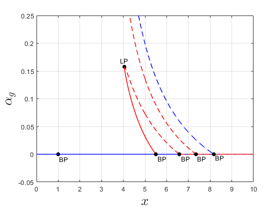
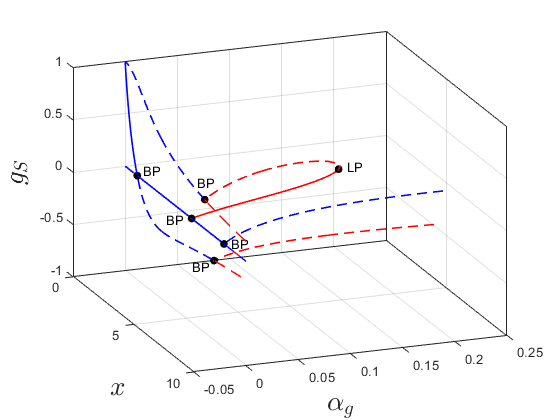
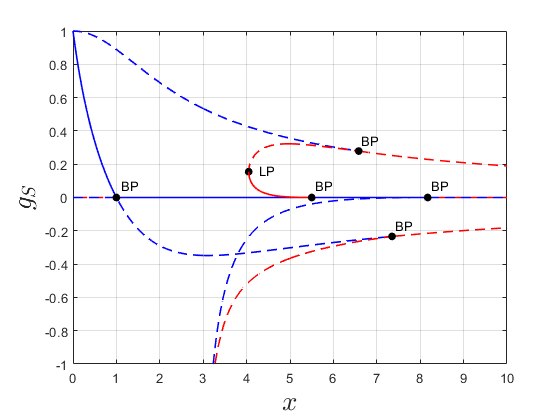
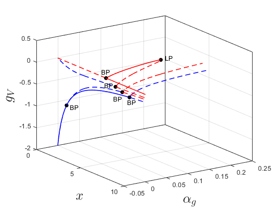
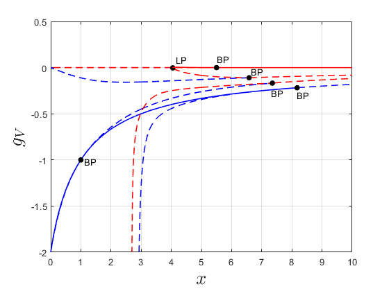
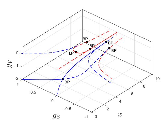
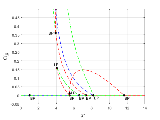
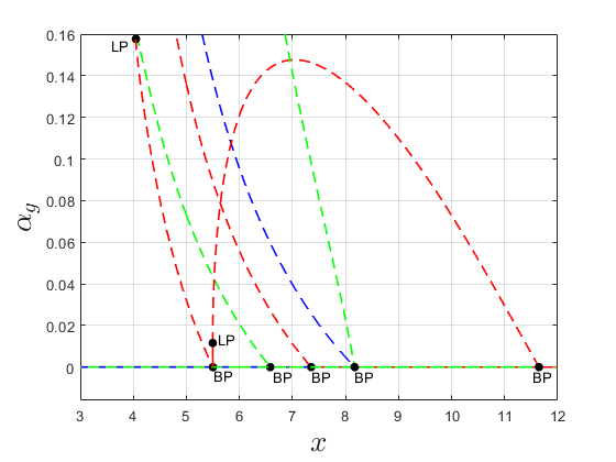
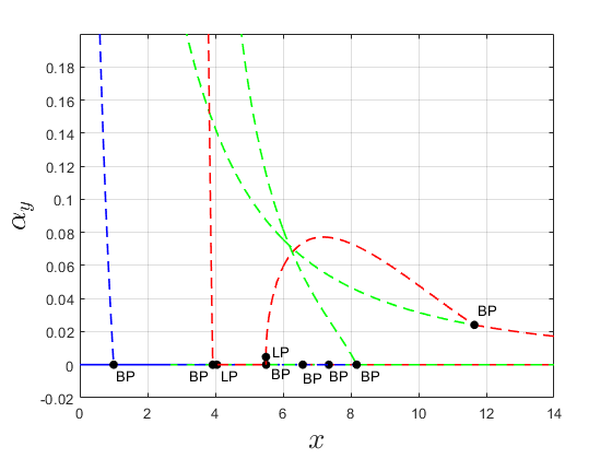
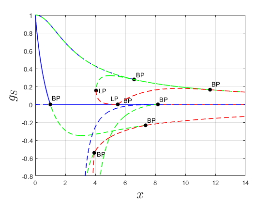
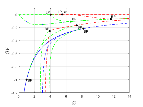
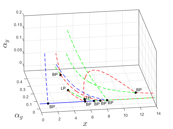
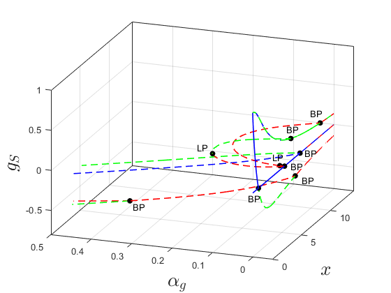
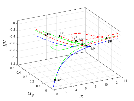
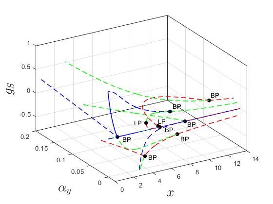
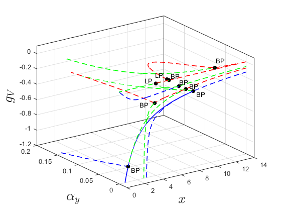
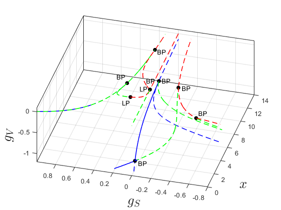
The behavior of the fixed points projected on the (x,αg)𝑥subscript𝛼𝑔(x,\alpha_{g}), (x,gS)𝑥subscript𝑔𝑆(x,g_{S}), (x,gV)𝑥subscript𝑔𝑉(x,g_{V}) planes and (x,αg,gS)𝑥subscript𝛼𝑔subscript𝑔𝑆(x,\alpha_{g},g_{S}), (x,αg,gV)𝑥subscript𝛼𝑔subscript𝑔𝑉(x,\alpha_{g},g_{V}) and (x,gS,gV)𝑥subscript𝑔𝑆subscript𝑔𝑉(x,g_{S},g_{V}) spaces are shown in Figure 2. We use the following color coding in this figure:

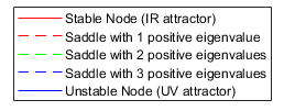
  • Solid red line: stable node, 3 negative eigenvalues (IR attractor).

  • Dashed red line: saddle point, 2 negative and 1 positive eigenvalue.

  • Dashed blue line: saddle point, 1 negative and 2 positive eigenvalues.

  • Solid blue line: unstable node, 3 positive eigenvalues (UV attractor).

The equilibria on the αg=0subscript𝛼𝑔0\alpha_{g}=0 manifold all have a trivial eigenvalue, and therefore do not fit the color coding as described above. In order to use the color coding, we define the sign of a trivial eigenvalue on this manifold by approaching the equilibrium along a line of constant gSsubscript𝑔𝑆g_{S} and gVsubscript𝑔𝑉g_{V} from positive but small αgsubscript𝛼𝑔\alpha_{g}. The trivial eigenvalue will then approach 00 from either positive or negative values. If the trivial eigenvalue is slightly positive for 0<αg10subscript𝛼𝑔much-less-than10<\alpha_{g}\ll 1, we define the trivial eigenvalue to be positive and vice versa.444This definition makes physical sense, since negative values of αgsubscript𝛼𝑔\alpha_{g} are unphysical.

Refer to caption
Refer to caption
Refer to caption
Refer to caption
Refer to caption
Refer to caption
Refer to caption
Figure 2: The fixed points of the RG-flow of (15) projected on the (x,αg)𝑥subscript𝛼𝑔(x,\alpha_{g})-plane, (x,gS)𝑥subscript𝑔𝑆(x,g_{S})-plane, (x,gV)𝑥subscript𝑔𝑉(x,g_{V})-plane, (x,αg,gS)𝑥subscript𝛼𝑔subscript𝑔𝑆(x,\alpha_{g},g_{S})-space, (x,αg,gV)𝑥subscript𝛼𝑔subscript𝑔𝑉(x,\alpha_{g},g_{V})-space and the (x,gS,gV)𝑥subscript𝑔𝑆subscript𝑔𝑉(x,g_{S},g_{V})-space. LP: Limit Point. BP: Branching Point.

In Figure 2, 4 up to 8 equilibria are shown, depending on the value of x𝑥x. Furthermore, a few bifurcations are found. The parameter and coordinate values of these bifurcations are reported in Table 1. The Branching points all correspond to transcritical bifurcations. The transcritical bifurcation at x=1𝑥1x=1 is located in the subspace αg=0subscript𝛼𝑔0\alpha_{g}=0, while the other transcritical bifurcations are located on the intersection of the subspaces αg=0subscript𝛼𝑔0\alpha_{g}=0 and αg=αgntsubscript𝛼𝑔superscriptsubscript𝛼𝑔𝑛𝑡\alpha_{g}=\alpha_{g}^{nt}. In the latter case, both a trivial and a non-trivial equilibrium555We call a fixed point trivial, if it has a trivial αgsubscript𝛼𝑔\alpha_{g} value and non-trivial otherwise. are involved. At all the non-trivial equilibria, the equilibrium has a positive eigenvalue, when αg<0subscript𝛼𝑔0\alpha_{g}<0, that becomes negative when αg>0subscript𝛼𝑔0\alpha_{g}>0, while the trivial equilibrium has a negative eigenvalue that becomes positive. At the branching point at x=5.5𝑥5.5x=5.5 a stable node with αg>0subscript𝛼𝑔0\alpha_{g}>0 is created. This indicates the upper edge of the conformal window as discussed in the introduction of this section. Finally, at x=4.05𝑥4.05x=4.05 two non-trivial equilibria collide and disappear through a saddle-node bifurcation (limit point). This saddle-node bifurcation could indicate the lower edge of the conformal window through a fixed point merger, as was discussed in [15] and [3]. The two other non-trivial fixed points diverge for x2.5less-than-or-similar-to𝑥2.5x\lesssim 2.5, close to the divergence of the large Ncsubscript𝑁𝑐N_{c} limit in equation (6).

Table 1: Locations of bifurcations found in model (15) for QCD4 in the Veneziano limit.
Bifurcation x𝑥x αgsubscript𝛼𝑔\alpha_{g} gSsubscript𝑔𝑆g_{S} gVsubscript𝑔𝑉g_{V}
Saddle-node 4.0494.0494.049 0.1580.1580.158 0.1550.1550.155 0.0030.003-0.003
Transcritical 1.0001.0001.000 00 00 1.0001.000-1.000
Transcritical 5.5015.5015.501 00 00 00
Transcritical 6.5826.5826.582 00 0.2790.2790.279 0.1100.110-0.110
Transcritical 7.3517.3517.351 00 0.2340.234-0.234 0.1680.168-0.168
Transcritical 8.1738.1738.173 00 00 0.2180.218-0.218

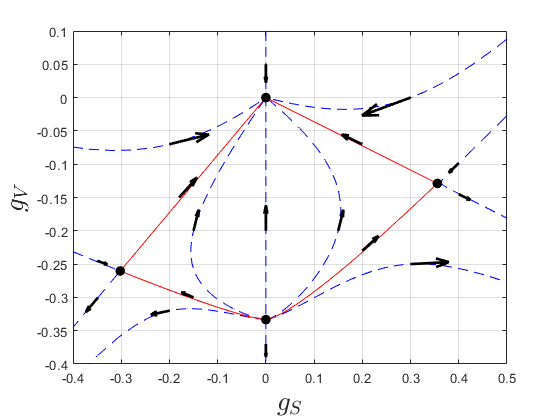
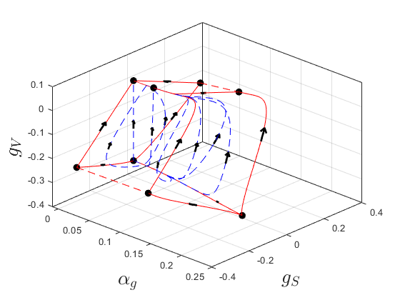
A few characteristic orbits of the RG-flow in the Veneziano limit are visualized in Figures 2.2, 2.2 and 2.2.

In Figure 2.2, a phase portrait on the invariant plane αg=0subscript𝛼𝑔0\alpha_{g}=0 is shown at x=5𝑥5x=5. We find 4 fixed points, and 4 red critical heteroclinic orbits, connecting those fixed points, and marking the boundaries of an invariant set. All orbits inside this set have a finite UV and finite IR fixed point, while orbits outside the invariant set have a diverging IR limit or diverging UV limit. The structure of this flow does not change, when x𝑥x is varied in the region x>1𝑥1x>1. Only the location of the fixed points and connecting orbits will change continuously. At x=1𝑥1x=1, the two fixed points with smallest value of gVsubscript𝑔𝑉g_{V} collide and exchange stability, via a transcritical bifurcation, yielding a similar phase portrait.

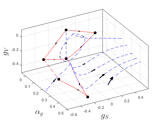
In Figure 2.2, a phase portrait of the flow in the 3-dimensional space is shown at x=5𝑥5x=5. Here, all 8 fixed points are shown, together with a few heteroclinic orbits connecting them. The red heteroclinic orbits form a skeleton of a 3-dimensional invariant set. This invariant set is bound by six invariant planes. The solid red lines lie on the intersections of these planes. The dashed red lines indicate the presence of other intersections, of which the exact locations haven’t been found numerically. All orbits inside this set have a finite UV and IR fixed point, while orbits outside the invariant set have a diverging IR limit, a diverging UV limit or both. More precisely, the bulk of the invariant set consists of structurally stable orbits going from the equilibrium at (αg,gS,gV)=(0,0,0.333)subscript𝛼𝑔subscript𝑔𝑆subscript𝑔𝑉000.333(\alpha_{g},g_{S},g_{V})=(0,0,-0.333) to the equilibrium at (αg,gS,gV)=(0.032,0.003,0.000)subscript𝛼𝑔subscript𝑔𝑆subscript𝑔𝑉0.0320.0030.000(\alpha_{g},g_{S},g_{V})=(0.032,0.003,0.000), and the boundary planes consist of non-stable heteroclinic orbits between the other fixed points. Within the invariant set the theory is in a chirally symmetric phase, while outside the set the chiral symmetry is broken. The structure of this flow does not change when x𝑥x is varied in the region 4.05<x<5.54.05𝑥5.54.05<x<5.5. Only the location of the fixed points and connecting orbits will change continuously. At x=4.05𝑥4.05x=4.05 the two fixed points shown at (αg,gS,gV)=(0.032,0.003,0.000)subscript𝛼𝑔subscript𝑔𝑆subscript𝑔𝑉0.0320.0030.000(\alpha_{g},g_{S},g_{V})=(0.032,0.003,0.000) and (αg,gS,gV)=(0.073,0.322,0.084)subscript𝛼𝑔subscript𝑔𝑆subscript𝑔𝑉0.0730.3220.084(\alpha_{g},g_{S},g_{V})=(0.073,0.322,-0.084) disappear through a saddle-node bifurcation.

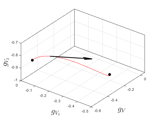
In Figure 2.2, a phase portrait in the whole space is shown at x=4𝑥4x=4. Here, only 6 fixed points are left. The six fixed points together span two unstable bounded 2-dimensional invariant sets. The solid red lines border these sets, and the dashed red line indicates the location, where the last border is expected, which hasn’t been found numerically. The 3-dimensional invariant set, which was present at x=5𝑥5x=5, has been broken down at the saddle-node bifurcation to two 2-dimensional invariant planes. The structure of the flow does not change when x𝑥x is varied in the region 0<x<4.050𝑥4.050<x<4.05, but the two non-trivial fixed points diverge when x𝑥x is lowered towards x=2.5𝑥2.5x=2.5. The orbits outside of the invariant planes all diverge in the IR limit. The eigenvector with 00 eigenvalue at the saddle-node bifurcation666This eigenvector is directly related to the operator that crosses marginality. is mainly directed in the gSsubscript𝑔𝑆g_{S} direction, as can be found in Table 2. Therefore, the divergence is the strongest in the gSsubscript𝑔𝑆g_{S} direction, indicating that the chiral symmetry is broken due to the scalar part of the four-fermi interaction, as discussed in [35]. Furthermore, we notice that there still exist chirally symmetric trajectories with a zero UV and finite IR limit, but these are unstable, and therefore need a very precise fine-tuning within this model.

Table 2: Eigenvalues and eigenvectors at the saddle-node bifurcation at x=4.049𝑥4.049x=4.049.
Eigenvalue Normalized eigenvector w.r.t the basis {eα,eS,eV}subscript𝑒𝛼subscript𝑒𝑆subscript𝑒𝑉\{e_{\alpha},e_{S},e_{V}\}
00 (0.09, 0.98,0.15)0.090.980.15(0.09,\;0.98,-0.15)
0.560.56-0.56 (0.19,0.95, 0.24)0.190.950.24(0.19,-0.95,\;0.24)
2.132.13-2.13 (0.10, 0.50, 0.86)0.100.500.86(0.10,\;0.50,\;0.86)
Refer to caption
(a) Phase portrait of the RG-flow in the (gS,gV)subscript𝑔𝑆subscript𝑔𝑉(g_{S},g_{V})-plane for αg=0subscript𝛼𝑔0\alpha_{g}=0 in the Veneziano limit at x=5𝑥5x=5. Solid red lines indicate the boundaries of an invariant set.
Refer to caption
(b) Phase portrait of the RG-flow in the (αg,gS,gV)subscript𝛼𝑔subscript𝑔𝑆subscript𝑔𝑉(\alpha_{g},g_{S},g_{V})-space in the Veneziano limit at x=5𝑥5x=5. Red lines indicates the skeleton of an invariant set.
Refer to caption
(c) Phase portrait of the RG-flow in the (αg,gS,gV)subscript𝛼𝑔subscript𝑔𝑆subscript𝑔𝑉(\alpha_{g},g_{S},g_{V})-space in the Veneziano limit at x=4𝑥4x=4. Red lines indicate the boundaries of 2-dimensional invariant sets.

2.3 Small Ncsubscript𝑁𝑐N_{c} regime

2.3.1 Fixed points and Codim-1 bifurcations

In the model out of the Veneziano limit there are 2 bifurcation parameters Ncsubscript𝑁𝑐N_{c} and x=Nf/Nc𝑥subscript𝑁𝑓subscript𝑁𝑐x=N_{f}/N_{c}, which allows for more interesting types of bifurcations. Again, we are interested in the renormalized trajectories of the theory and the invariant sets enclosed by the renormalized trajectories, indicating the existence of chirally symmetric theories. We have numerically found that the model contains up to 20 different real fixed points with αg0subscript𝛼𝑔0\alpha_{g}\geq 0 for integer values of (Nc,Nf)[1,10]×[1,100]subscript𝑁𝑐subscript𝑁𝑓1101100(N_{c},N_{f})\in[1,10]\times[1,100]. The beta function for αgsubscript𝛼𝑔\alpha_{g} yields two roots

αg=0,αg=αgnt:=Nc211+2x+3xgV34Nc213xNc2+3x,formulae-sequencesubscript𝛼𝑔0subscript𝛼𝑔superscriptsubscript𝛼𝑔𝑛𝑡assignsuperscriptsubscript𝑁𝑐2112𝑥3𝑥subscript𝑔𝑉34superscriptsubscript𝑁𝑐213𝑥superscriptsubscript𝑁𝑐23𝑥\alpha_{g}=0,\quad\alpha_{g}=\alpha_{g}^{nt}:=N_{c}^{2}\frac{-11+2x+3xg_{V}}{34N_{c}^{2}-13xN_{c}^{2}+3x},

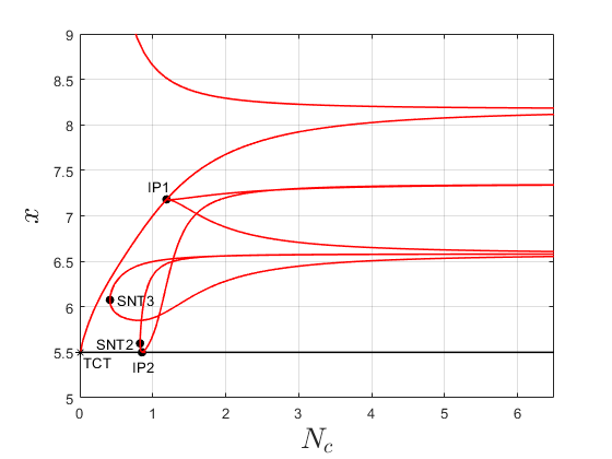
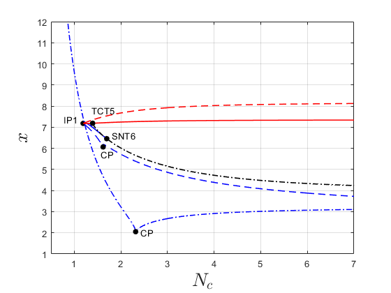
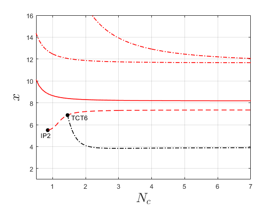
where the trivial root has multiplicity two. The (αg=0)subscript𝛼𝑔0(\alpha_{g}=0)-hyperplane is an invariant set of the model, which allows to study the model without gauge interactions separately. Setting αg=0subscript𝛼𝑔0\alpha_{g}=0, we find up to 12 fixed points, which can be continued using MatCont. Two of those disappear through a saddle-node bifurcation at x>7.5𝑥7.5x>7.5, which is above the conformal window. The 10 remaining fixed points play an important role for the behavior for αg0subscript𝛼𝑔0\alpha_{g}\neq 0. For every of these ten fixed points, we find a related fixed point on the manifold αg=αgntsubscript𝛼𝑔superscriptsubscript𝛼𝑔𝑛𝑡\alpha_{g}=\alpha_{g}^{nt}. For large values of x𝑥x all the non-trivial fixed points have αg<0subscript𝛼𝑔0\alpha_{g}<0, but for smaller values of x𝑥x they have αg>0subscript𝛼𝑔0\alpha_{g}>0, and become physically relevant. On the intersection of the two hyperplanes, where αg=αgnt=0subscript𝛼𝑔superscriptsubscript𝛼𝑔𝑛𝑡0\alpha_{g}=\alpha_{g}^{nt}=0, i.e. when x=112+3gV𝑥1123subscript𝑔𝑉x=\frac{11}{2+3g_{V}}, all non-trivial fixed points collide with a trivial fixed point, through a transcritical bifurcation. The lines at which these transcritical bifurcations occur are shown in Figure 3. Using the transcritical bifurcations, we relate all the non-trivial fixed points to a trivial fixed point.

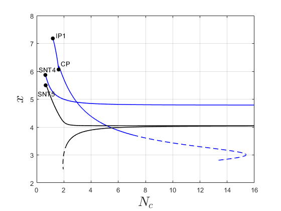
The 10 non-trivial fixed points with positive αgsubscript𝛼𝑔\alpha_{g} exist for large values of x𝑥x. However, for small values, they either disappear through a saddle-node bifurcation or diverge in one or multiple couplings. In Figure 3 the saddle-node bifurcation lines are shown. Here, we see that two pairs (black lines) of fixed points will disappear through a saddle-node bifurcation which is connected to the saddle-node bifurcation that was found in the Veneziano limit777There were in fact two saddle-node bifurcations in the Veneziano limit with differing (gV1,gV2)subscript𝑔subscript𝑉1subscript𝑔subscript𝑉2(g_{V_{1}},g_{V_{2}}). They were reported as one since the beta functions for gV1subscript𝑔subscript𝑉1g_{V_{1}} and gV2subscript𝑔subscript𝑉2g_{V_{2}} decoupled and weren’t considered. The two bifurcation curves are close together for large Ncsubscript𝑁𝑐N_{c}, but split up at small Ncsubscript𝑁𝑐N_{c}. One of the curves starts to increase steeply around Nc=2subscript𝑁𝑐2N_{c}=2, while the other starts decreasing around Nc=6subscript𝑁𝑐6N_{c}=6, and diverges in the coupling constants at Nc=2subscript𝑁𝑐2N_{c}=2. Therefore the saddle-node bifurcation of this pair does not exist for Nc=1subscript𝑁𝑐1N_{c}=1, and the fixed points diverge instead. Then there is a third pair of fixed points (upper blue line) that disappears through a saddle-node bifurcation for all Ncsubscript𝑁𝑐N_{c} around x=4.8𝑥4.8x=4.8. However this value starts to increase around Nc=4subscript𝑁𝑐4N_{c}=4. A fourth pair disappears through a saddle-node bifurcation when 1<Nc<161subscript𝑁𝑐161<N_{c}<16, diverges for Nc16subscript𝑁𝑐16N_{c}\geq 16, while at Nc=1subscript𝑁𝑐1N_{c}=1 the fixed points will not exist for positive αgsubscript𝛼𝑔\alpha_{g}. The last two fixed points do not disappear through a saddle-node bifurcation, but will diverge in multiple couplings at small x𝑥x.

Refer to caption
(d) Transcritical bifurcations on the intersection of the (αg=0)subscript𝛼𝑔0(\alpha_{g}=0) and (αg=αgnt)subscript𝛼𝑔superscriptsubscript𝛼𝑔𝑛𝑡(\alpha_{g}=\alpha_{g}^{nt}) subspaces. Black line: transcritical bifurcation marking the upper edge of the conformal window bifurcation curves.
Refer to caption
(e) Saddle-node bifurcations in the (αg=αgnt0)subscript𝛼𝑔superscriptsubscript𝛼𝑔𝑛𝑡0(\alpha_{g}=\alpha_{g}^{nt}\geq 0)-subspace. Black lines: saddle-node bifurcation, that was also found in the Veneziano limit.
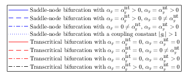
Figure 3: Bifurcations of the QCD4 model (13), shown in the (Nc,x)subscript𝑁𝑐𝑥(N_{c},x)-plane. Red Lines: transcritical bifurcations. Blue lines: saddle-node bifurcations. Dashed lines: bifurcation curves, with at least one of the coupling constants |gi|>1subscript𝑔𝑖1|g_{i}|>1. CP: Cusp bifurcation. SNT: Saddle-Node-Transcritical bifurcation. TCT: Transcritical-Transcritical bifurcation. IP: degenerate bifurcation point.

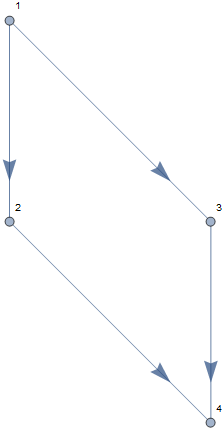
Using these saddle-node bifurcation curves, we can partition the 10 non-trivial fixed points into 5 pairs. Since all 10 non-trivial fixed points are related to a trivial fixed point through a transcritical bifurcation curve, we can partition the 20 fixed points into groups of 4 consisting of 2 trivial and 2 non-trivial fixed points. It turns out that the heteroclinic orbits between the fixed points within each of these sets have a similar topology, which is as shown in Figure 4: at first, for large x𝑥x, the two non-trivial fixed points lie below the αg=0subscript𝛼𝑔0\alpha_{g}=0 hyperplane, and the αg=0subscript𝛼𝑔0\alpha_{g}=0 hyperplane is locally attractive in the IR limit, then, at a specific value of x𝑥x, one of the non-trivial and one of the trivial fixed points collide through a transcritical bifurcation and the non-trivial fixed point gets a positive αgsubscript𝛼𝑔\alpha_{g} creating a locally attractive IR limit set bounded by orbits between the 3 fixed points with αg0subscript𝛼𝑔0\alpha_{g}\geq 0. Next, at smaller specific x𝑥x, the other non-trivial fixed point will collide with the other trivial fixed point and also get positive αgsubscript𝛼𝑔\alpha_{g} value. After this, at small x𝑥x, the non-trivial fixed points will either disappear through a saddle-node bifurcation or diverge, making the αg=0subscript𝛼𝑔0\alpha_{g}=0 hyperplane locally repulsive in the IR limit.

Refer to caption
Figure 4: Topology of the RG-flow between 4 fixed points in a group. Left (Large N): the 2 non-trivial fixed points have αg<0subscript𝛼𝑔0\alpha_{g}<0. Middle (intemediate N): One of the non-trivial fixed points has αg>0subscript𝛼𝑔0\alpha_{g}>0. Right (small N): Both of the non-trivial fixed points have αg>0subscript𝛼𝑔0\alpha_{g}>0.

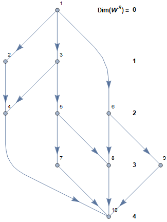
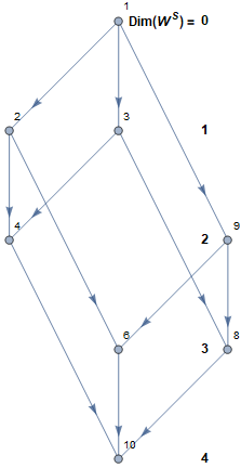
We can also visualize the structure of the flow on the invariant (αg=0)subscript𝛼𝑔0(\alpha_{g}=0)-space. A graphical representation of the fixed points and a few critical orbits is shown in Figure 5 for (Nc,Nf)=(3,15)subscript𝑁𝑐subscript𝑁𝑓315(N_{c},N_{f})=(3,15) and (Nc,Nf)=(3,3)subscript𝑁𝑐subscript𝑁𝑓33(N_{c},N_{f})=(3,3). We notice that two points (labeled by 5 and 7) do exist for (Nc,Nf)=(3,15)subscript𝑁𝑐subscript𝑁𝑓315(N_{c},N_{f})=(3,15), but do not exist for (Nc,Nf)=(3,3)subscript𝑁𝑐subscript𝑁𝑓33(N_{c},N_{f})=(3,3). This is due to a saddle-node bifurcation in the (αg=0)subscript𝛼𝑔0(\alpha_{g}=0)-space at (Nc,Nf)(3,5.9)subscript𝑁𝑐subscript𝑁𝑓35.9(N_{c},N_{f})\approx(3,5.9). Furthermore two fixed points (labeled by 6 and 9) have exchanged stability through a transcritical bifurcation at (Nc,Nf)(3,7.7)subscript𝑁𝑐subscript𝑁𝑓37.7(N_{c},N_{f})\approx(3,7.7). The curves corresponding to these two bifurcations are shown in Figure 6 and 6 respectively. In the remainder of this section, we’ll use the numbers as in Figure 5 to label the fixed points. Since we have related every trivial fixed point uniquely to a non-trivial fixed point, we give the non-trivial fixed point the same number as its trivial counterpart. However, we add the label ‘a’ to the trivial fixed points and the label ‘b’ to the non-trivial fixed points.
Refer to caption
Refer to caption
Figure 5: Stability of the fixed points and topology of the RG-flow between the fixed points on the four dimensional invariant set αg=0subscript𝛼𝑔0\alpha_{g}=0 at (Nc,Nf)=(3,15)subscript𝑁𝑐subscript𝑁𝑓315(N_{c},N_{f})=(3,15) (left), and at (Nc,Nf)=(3,3)subscript𝑁𝑐subscript𝑁𝑓33(N_{c},N_{f})=(3,3) (right). Bold numbers correspond to the dimension of the stable manifold at the fixed point.

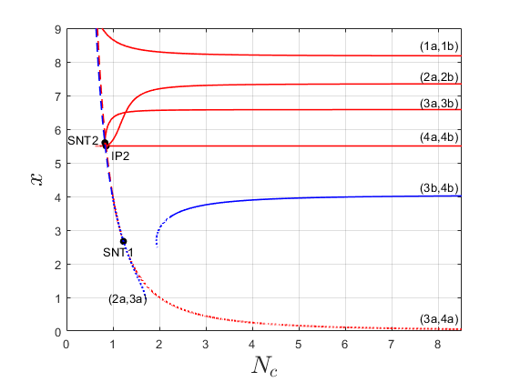
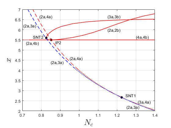
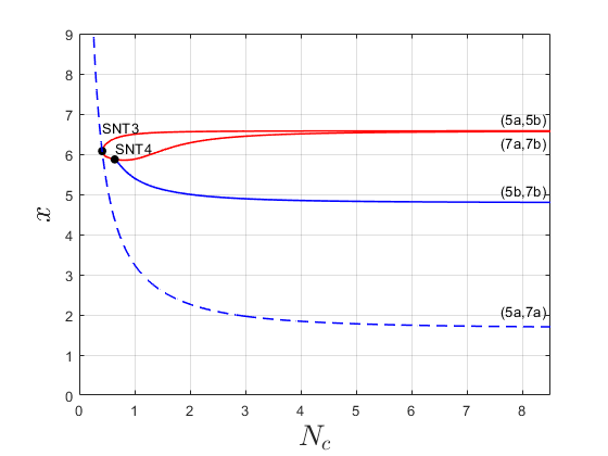
We have numerically found all local bifurcations888We have performed a quite extensive study, and therefore have great confidence that we found all local bifurcations in this region. Furthermore, we have not found any global bifurcations, and believe that there are none in the studied region. However, this is numerically harder to verify. involving these 20 fixed points for αg0subscript𝛼𝑔0\alpha_{g}\geq 0, and these are shown in Figure 6. This figure also includes the saddle-node and transcritical bifurcation curves shown in Figure 3.
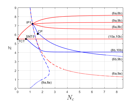
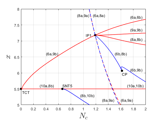
Refer to caption
(a) Fixed points 6,8,9,10; Nc[0,8.5]subscript𝑁𝑐08.5N_{c}\in[0,8.5].
Refer to caption
(b) Fixed points 6,8,9,10; Nc[0,2]subscript𝑁𝑐02N_{c}\in[0,2].
Refer to caption
(c) Fixed points 1,2,3,4; Nc[0,8.5]subscript𝑁𝑐08.5N_{c}\in[0,8.5].
Refer to caption
(d) Fixed points 1,2,3,4; Nc[0.7,1.4]subscript𝑁𝑐0.71.4N_{c}\in[0.7,1.4].
Refer to caption
(e) Fixed points 5,7; Nc[0,8.5]subscript𝑁𝑐08.5N_{c}\in[0,8.5].
Refer to caption
Figure 6: Bifurcations of various sets of fixed points in the QCD4 model (13) in the (Nc,x)subscript𝑁𝑐𝑥(N_{c},x)-plane. CP: Cusp bifurcation. SNT: Saddle-Node-Transcritical bifurcation. TCT: Transcritical-Transcritical bifurcation. IP: degenerate bifurcation point. Numbers indicate which equilibria are involved in the bifurcation, and correspond to the numbers in Figure 5.

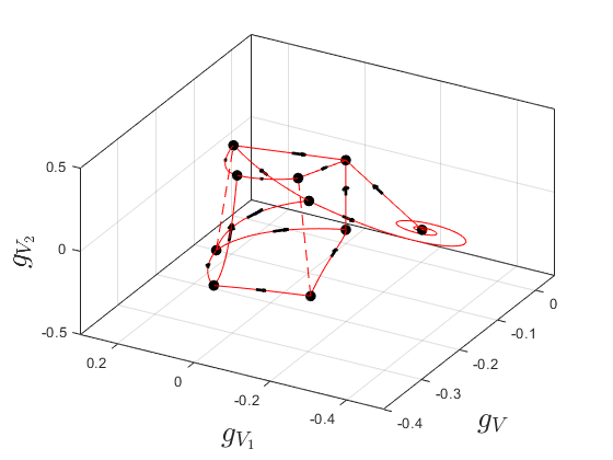
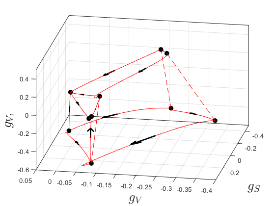
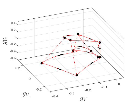
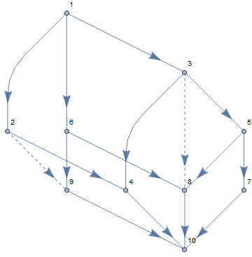
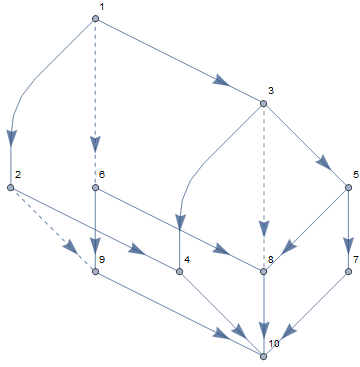
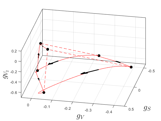
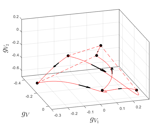
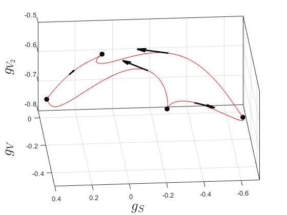
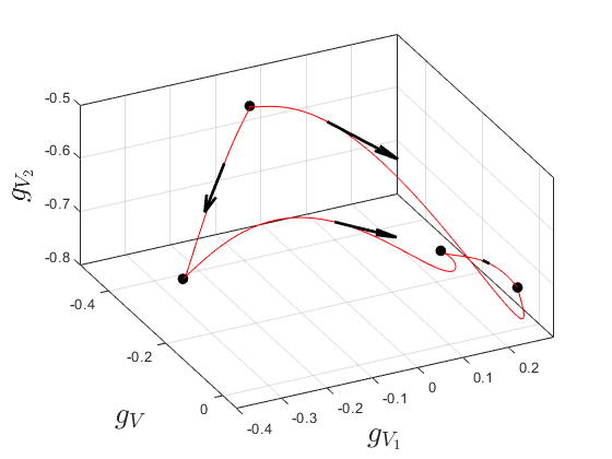
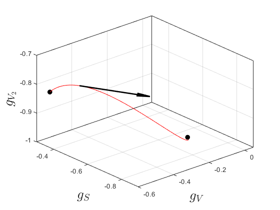
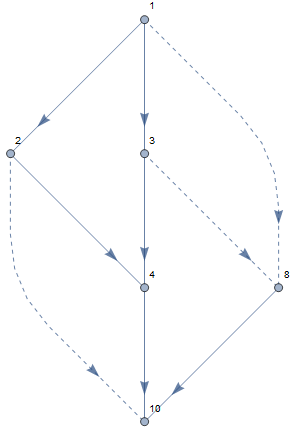
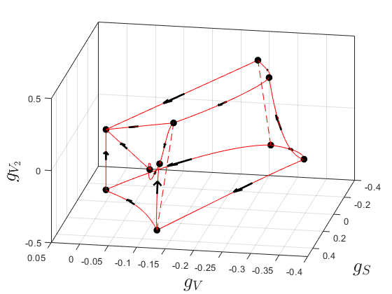
We use the bifurcation diagram 6 to distinguish and visualize several phases within the RG-flow generated by our model (10). For this, we set Nc=3subscript𝑁𝑐3N_{c}=3, and take Nf{11,12,13,15}subscript𝑁𝑓11121315N_{f}\in\{11,12,13,15\}. The topology on the invariant (αg=0)subscript𝛼𝑔0(\alpha_{g}=0)-space will be the same for these four values of x𝑥x, since there are no bifurcations in this region. Only the location of the fixed points will change continuously. Projections of the fixed points and a few heteroclinic orbits in this 4-dimensional invariant subspace, at αg=0subscript𝛼𝑔0\alpha_{g}=0, are shown in Figure 7. The fixed points and a few heteroclinic orbits in the αg=αgntsubscript𝛼𝑔superscriptsubscript𝛼𝑔𝑛𝑡\alpha_{g}=\alpha_{g}^{nt} subspace are shown in Figures 8, 10, 11 and 12. In Figures 9 and 13 these figures are shown in a graphical representation.

At Nf=15subscript𝑁𝑓15N_{f}=15, we see 10 fixed points and a few heteroclinic orbits connecting them, both in the αg=0subscript𝛼𝑔0\alpha_{g}=0 and the αg=αgntsubscript𝛼𝑔superscriptsubscript𝛼𝑔𝑛𝑡\alpha_{g}=\alpha_{g}^{nt} hyperplane. The red lines shown in the figures form part of a skeleton of a closed set in the 4-dimensional subspaces αg=0subscript𝛼𝑔0\alpha_{g}=0 and αg=αgntsubscript𝛼𝑔superscriptsubscript𝛼𝑔𝑛𝑡\alpha_{g}=\alpha_{g}^{nt}. These two 4-dimensional sets on αg=0subscript𝛼𝑔0\alpha_{g}=0 and αg=αgntsubscript𝛼𝑔superscriptsubscript𝛼𝑔𝑛𝑡\alpha_{g}=\alpha_{g}^{nt} form a 4-dimensional boundary of a larger 5-dimensional invariant subspace of the full 5-dimensional space. The other 4-dimensional subspaces that bound the full 5-dimensional invariant set are spanned by orbits going from αg=0subscript𝛼𝑔0\alpha_{g}=0 towards αg=αgntsubscript𝛼𝑔superscriptsubscript𝛼𝑔𝑛𝑡\alpha_{g}=\alpha_{g}^{nt}. Dashed red lines indicate parts of the skeleton that haven’t been found numerically, but are expected to exist. The flow within the 5-dimensional invariant set is everywhere directed from the αg=0subscript𝛼𝑔0\alpha_{g}=0 towards the αg=αgnt>0subscript𝛼𝑔superscriptsubscript𝛼𝑔𝑛𝑡0\alpha_{g}=\alpha_{g}^{nt}>0 subspace. This set consists of structurally stable renormalized trajectories that have finite UV (with trivial αgsubscript𝛼𝑔\alpha_{g}) and IR limits (with strictly positive αgsubscript𝛼𝑔\alpha_{g}) indicating the theory to be in a symmetric phase. Outside the set, orbits have diverging IR and/or UV limit, and theories will have a broken chiral symmetry. The boundaries consist of unstable orbits between other fixed points, and therefore indicate unstable symmetric theories.

When the flavor number is reduced just below Nf=15subscript𝑁𝑓15N_{f}=15, at Nf=14.7subscript𝑁𝑓14.7N_{f}=14.7 and Nf=14.6subscript𝑁𝑓14.6N_{f}=14.6, two pairs of fixed points disappear through a saddle-node bifurcation. Because of these bifurcations, the invariant set of orbits indicating symmetric theories is reduced. However, the most attractive IR fixed point with dim(Ws)=5dimensionsuperscript𝑊𝑠5\dim(W^{s})=5 still exists. This indicates that the invariant set is locally attractive in the IR limit. Reducing the flavor number even further to Nf=12subscript𝑁𝑓12N_{f}=12 and Nf=11subscript𝑁𝑓11N_{f}=11 more fixed points disappear through a saddle-node bifurcations. The invariant set of orbits at αg=αgntsubscript𝛼𝑔superscriptsubscript𝛼𝑔𝑛𝑡\alpha_{g}=\alpha_{g}^{nt} is reduced at every step, and therefore the set of asymptotically stable orbits with finite UV and IR limit becomes smaller, making the set of possible symmetric theories smaller. For Nf12.2subscript𝑁𝑓12.2N_{f}\leq 12.2, there is no fixed point left with dim(Ws)=5dimensionsuperscript𝑊𝑠5\dim(W^{s})=5. Therefore, the remaining invariant set is not an IR attractor anymore. Furthermore, we expect that the dimension of the invariant set with finite trajectories reduces, when more fixed points have disappeared through a saddle-node bifurcation. When the invariant set splits up into multiple invariant sets with dimension smaller than 555, symmetric theories only exist within this model under extreme fine-tuning. This is a strong indication that the lower edge of the conformal window has been crossed.

In Figure 7, there is another peculiarity visible. Here we see a heteroclinic orbit with spiraling behavior indicating the existence of renormalized trajectories with complex scaling behavior in and close to the αg=0subscript𝛼𝑔0\alpha_{g}=0 hyperplane. Equilibrium 5 and 7 are associated to this behavior.
Refer to caption
Refer to caption
Figure 7: Fixed points and critical heteroclinic orbits in the QCD4 model (13) at (Nc,Nf)=(3,15)subscript𝑁𝑐subscript𝑁𝑓315(N_{c},N_{f})=(3,15) and αg=0subscript𝛼𝑔0\alpha_{g}=0. Solid line: heteroclinic connections. Dashed lines: heteroclinic connections that are expected to exist, but haven’t been found numerically. Left: projection on the (gS,gV,gV2)subscript𝑔𝑆subscript𝑔𝑉subscript𝑔subscript𝑉2(g_{S},g_{V},g_{V_{2}})-space. Right: projection on the (gV,gV1,gV2)subscript𝑔𝑉subscript𝑔subscript𝑉1subscript𝑔subscript𝑉2(g_{V},g_{V_{1}},g_{V_{2}})-space.
Refer to caption
Refer to caption
Figure 8: Fixed points and critical heteroclinic orbits in the QCD4 model (13) at (Nc,Nf)=(3,15)subscript𝑁𝑐subscript𝑁𝑓315(N_{c},N_{f})=(3,15) and αg=αgntsubscript𝛼𝑔superscriptsubscript𝛼𝑔𝑛𝑡\alpha_{g}=\alpha_{g}^{nt}. Solid line: heteroclinic connections. Dashed lines: heteroclinic connections that are expected to exist, but haven’t been found numerically. Left: projection on the (gS,gV,gV2)subscript𝑔𝑆subscript𝑔𝑉subscript𝑔subscript𝑉2(g_{S},g_{V},g_{V_{2}})-space. Right: projection on the (gV,gV1,gV2)subscript𝑔𝑉subscript𝑔subscript𝑉1subscript𝑔subscript𝑉2(g_{V},g_{V_{1}},g_{V_{2}})-space.
Refer to caption
(a) Topology of the RG-flow at αg=0subscript𝛼𝑔0\alpha_{g}=0 corresponding to figure 7.
Refer to caption
(b) Topology of the RG-flow at αg=αgntsubscript𝛼𝑔superscriptsubscript𝛼𝑔𝑛𝑡\alpha_{g}=\alpha_{g}^{nt} corresponding to figure 8.
Figure 9: Graphical representation of the fixed points and the skeleton of the invariant set at (Nc,Nf)=(3,15)subscript𝑁𝑐subscript𝑁𝑓315(N_{c},N_{f})=(3,15) both on the αg=0subscript𝛼𝑔0\alpha_{g}=0 and the αg=αgntsubscript𝛼𝑔superscriptsubscript𝛼𝑔𝑛𝑡\alpha_{g}=\alpha_{g}^{nt} subspaces.
Refer to caption
Refer to caption
Figure 10: Fixed points and critical heteroclinic orbits of the QCD4 model (13) at (Nc,Nf)=(3,13)subscript𝑁𝑐subscript𝑁𝑓313(N_{c},N_{f})=(3,13) and αg=αgntsubscript𝛼𝑔superscriptsubscript𝛼𝑔𝑛𝑡\alpha_{g}=\alpha_{g}^{nt}. Solid line: heteroclinic connections. Dashed lines: heteroclinic connections that are expected to exist, but haven’t been found numerically. Left: projection on the (gS,gV,gV2)subscript𝑔𝑆subscript𝑔𝑉subscript𝑔subscript𝑉2(g_{S},g_{V},g_{V_{2}})-space. Right: projection on the (gV,gV1,gV2)subscript𝑔𝑉subscript𝑔subscript𝑉1subscript𝑔subscript𝑉2(g_{V},g_{V_{1}},g_{V_{2}})-space.
Refer to caption
Refer to caption
Figure 11: Fixed points and critical heteroclinic orbits of the QCD4 model (13) at (Nc,Nf)=(3,12)subscript𝑁𝑐subscript𝑁𝑓312(N_{c},N_{f})=(3,12) and αg=αgntsubscript𝛼𝑔superscriptsubscript𝛼𝑔𝑛𝑡\alpha_{g}=\alpha_{g}^{nt}. Left: projection on the (gS,gV,gV2)subscript𝑔𝑆subscript𝑔𝑉subscript𝑔subscript𝑉2(g_{S},g_{V},g_{V_{2}})-space. Right: projection on the (gV,gV1,gV2)subscript𝑔𝑉subscript𝑔subscript𝑉1subscript𝑔subscript𝑉2(g_{V},g_{V_{1}},g_{V_{2}})-space.
Refer to caption
Refer to caption
Figure 12: Fixed points and a critical heteroclinic orbit of the QCD4 model (13) at (Nc,Nf)=(3,11)subscript𝑁𝑐subscript𝑁𝑓311(N_{c},N_{f})=(3,11) and αg=αgntsubscript𝛼𝑔superscriptsubscript𝛼𝑔𝑛𝑡\alpha_{g}=\alpha_{g}^{nt}. Left: projection on the (gS,gV,gV2)subscript𝑔𝑆subscript𝑔𝑉subscript𝑔subscript𝑉2(g_{S},g_{V},g_{V_{2}})-space. Right: projection on the (gV,gV1,gV2)subscript𝑔𝑉subscript𝑔subscript𝑉1subscript𝑔subscript𝑉2(g_{V},g_{V_{1}},g_{V_{2}})-space.
Refer to caption
(a) Topology of the RG-flow Nf=13subscript𝑁𝑓13N_{f}=13 corresponding to figure 10.
Refer to caption
(b) Topology of the RG-flow Nf=12subscript𝑁𝑓12N_{f}=12 corresponding to figure 11.
Refer to caption
(c) Topology of the RG-flow Nf=11subscript𝑁𝑓11N_{f}=11 corresponding to figure 12.
Figure 13: Graphical representation of the fixed points and the skeleton of the invariant set on the αg=αgntsubscript𝛼𝑔superscriptsubscript𝛼𝑔𝑛𝑡\alpha_{g}=\alpha_{g}^{nt} subspace at Nc=3subscript𝑁𝑐3N_{c}=3 and various values of Nfsubscript𝑁𝑓N_{f}.

2.3.2 Operators crossing marginality and degenerate bifurcations

We have found 4 saddle-node bifurcation curves (cf. figure 3, 6) with non-trivial value of αgsubscript𝛼𝑔\alpha_{g}. All four indicate the disappearance of two fixed points when the value of x𝑥x is decreased. Along these curves we can identify the eigenvector corresponding to a zero eigenvalue as the relevant operator that crosses marginality. These critical eigenvectors at Nc=3subscript𝑁𝑐3N_{c}=3 are reported in Table 3. We have found that these operators are very dependent on x𝑥x, but not on Ncsubscript𝑁𝑐N_{c}. From the table we conclude that 3 of the saddle-node bifurcations have 2 complex eigenvalues at Nc=3subscript𝑁𝑐3N_{c}=3, while one has only real eigenvalues. We notice that the normalized eigenvectors corresponding to the complex eigenvalues are all directed along the four-fermi couplings, and have very small contributions (|ηαg|<0.007subscript𝜂subscript𝛼𝑔0.007|\eta_{\alpha_{g}}|<0.007) along the eαgsubscript𝑒subscript𝛼𝑔e_{\alpha_{g}} direction, meaning that this complex scaling behavior involves operators, which are linear combinations of the effective four-fermi interactions. Furthermore, we see that the operator crossing marginality is a linear combination of all operators. However the scalar four-fermi interaction is most relevant in three of the saddle-node bifurcations, while in the saddle-node bifurcation of equilibria 5b and 7b the V1subscript𝑉1V_{1} interaction is most relevant.

Table 3: Eigenvalues and critical eigenvectors crossing marginality of the saddle-node bifurcation with non-trivial αgsubscript𝛼𝑔\alpha_{g} at Nc=3subscript𝑁𝑐3N_{c}=3.
Equilibria (Nc,x)subscript𝑁𝑐𝑥(N_{c},x) Eigenvalues Critical eigenvector
8, 10 (3.00,4.06)3.004.06(3.00,4.06) {2.88,2.10,1.36,0.64,0}2.882.101.360.640\{-2.88,-2.10,-1.36,-0.64,0\} (0.12,0.94,0.17,0.12, 0.22)0.120.940.170.120.22(0.12,0.94,-0.17,0.12,\;0.22)
6, 9 (3.00,4.86)3.004.86(3.00,4.86) {3.62±0.27i,1.79,0.62,0}plus-or-minus3.620.27𝑖1.790.620\{-3.62\pm 0.27i,1.79,-0.62,0\} (0.11,0.86,0.21,0.35, 0.28)0.110.860.210.350.28(0.11,0.86,-0.21,0.35,\;0.28)
3, 4 (3.00,3.75)3.003.75(3.00,3.75) {3.38±1.05i,2.57,0.81,0}plus-or-minus3.381.05𝑖2.570.810\{3.38\pm 1.05i,-2.57,-0.81,0\} (0.07,0.77,0.08,0.50,0.38)0.070.770.080.500.38(0.07,0.77,-0.08,0.50,-0.38)
5, 7 (3.00,4.89)3.004.89(3.00,4.89) {1.66±0.09i,1.59,0.27,0}plus-or-minus1.660.09𝑖1.590.270\{-1.66\pm 0.09i,1.59,-0.27,0\} (0.04,0.06,0.07,0.95, 0.28)0.040.060.070.950.28(0.04,0.06,-0.07,0.95,\;0.28)

In the complete model we have encountered nine bifurcation points with higher codimension. An overview can be found in Table 4. Six of these points lie in the physical uninteresting region Nc(0,1)subscript𝑁𝑐01N_{c}\in(0,1), while three of them (CP, SNT1 and IP1) may have physical relevance, since Nc1subscript𝑁𝑐1N_{c}\geq 1. Those points will be discussed below. The point labeled with ‘CP’ corresponds to a cusp bifurcation and the points labeled with ‘SNT’ correspond to saddle-node-transcritical bifurcations, as discussed in Appendix A. The point ‘TCT’ labels an intersection of two independent transcritical bifurcation curves and corresponds to the normal form

{x˙=αx+x2,y˙=βy+y2.cases˙𝑥𝛼𝑥superscript𝑥2otherwise˙𝑦𝛽𝑦superscript𝑦2otherwise\begin{cases}\dot{x}=\alpha x+x^{2},\\ \dot{y}=\beta y+y^{2}.\end{cases} (16)

The points ‘IP’ label more degenerate bifurcation points.

Table 4: Locations of bifurcations found in the model of QCD4 (15) with effective four-fermi interactions.
Bifurcation Ncsubscript𝑁𝑐N_{c} Nfsubscript𝑁𝑓N_{f} x𝑥x αgsubscript𝛼𝑔\alpha_{g} gSsubscript𝑔𝑆g_{S} gVsubscript𝑔𝑉g_{V} gV1subscript𝑔subscript𝑉1g_{V_{1}} gV2subscript𝑔subscript𝑉2g_{V_{2}}
CP 1.621.621.62 9.829.829.82 6.076.076.07 0.050.050.05 0.030.030.03 0.170.17-0.17 0.010.010.01 0.220.220.22
SNT1 1.221.221.22 3.273.273.27 2.672.672.67 00 00 00 00 1.501.50-1.50
SNT2 0.830.830.83 4.634.634.63 5.605.605.60 00 0.280.280.28 0.010.01-0.01 0.120.120.12 0.820.82-0.82
SNT3 0.410.410.41 2.512.512.51 6.086.086.08 00 0.280.280.28 0.060.06-0.06 0.020.02-0.02 0.010.01-0.01
SNT4 0.640.640.64 3.763.763.76 5.875.875.87 00 0.260.260.26 0.040.04-0.04 0.050.05-0.05 0.040.04-0.04
SNT5 0.660.660.66 3.653.653.65 5.505.505.50 00 00 00 00 00
TCT 00 00 00 00 00 00 00 00
IP1 1.191.191.19 8.548.548.54 7.187.187.18 00 00 0.160.16-0.16 00 0.170.170.17
IP2 0.850.850.85 4.694.694.69 5.505.505.50 00 00 00 00 0.730.73-0.73

At the cusp bifurcation 2 saddle-node bifurcation curves with non-trivial value of αgsubscript𝛼𝑔\alpha_{g} meet. The first curve is associated to the pair of equilibria (6b,8b) and the second to (6b,9b).

The point SNT1, describes a saddle-node-transcritical bifurcation, of a saddle-node curve that lies in the subspace αg=0subscript𝛼𝑔0\alpha_{g}=0 and involves the equilibria (2a,3a), and two transcritical curves that also lie in the αg=0subscript𝛼𝑔0\alpha_{g}=0 subspace and involve the equilibria (2a,4a) and (3a,4a).

IP1 is a highly degenerate bifurcation point. The model reduced on the invariant subspace αg=0subscript𝛼𝑔0\alpha_{g}=0 has a pitchfork bifurcation at this point. However, in the 5-dimensional model the branches of the equilibrium curves meeting at this pitchfork bifurcation are all transcritical bifurcation curves of the equilibria (6a,6b), (8a,8b), (9a,9b) and (6a,9b). In addition, to this pitchfork bifurcation we find a saddle-node-transcritical bifurcation at this point. The curves associated to this saddle-node-transcritical bifurcation all lie in the αg=0subscript𝛼𝑔0\alpha_{g}=0 subspace. The saddle-node curve involves the equilibria (8a,9a) and the branches of the transcritical bifurcation involve (6a,8a) and (6a,9a).999This is still a bit speculative. We expect the pitchfork bifurcation and the saddle-node-transcritical bifurcation to overlap, but this is hard to verify numerically. On top of this, there is a saddle-node bifurcation curve with non-trivial αgsubscript𝛼𝑔\alpha_{g} intersecting at this point. This curve involves the equilibria (6b,8b). Together with the branches of transcritical bifurcation curves of (6a,6b) and (8a,8b), that were contained in the pitchfork bifurcation, we could also see this point as saddle-node-transcritical bifurcation of these points. In short this point is highly degenerate and can be unfolded into two saddle-node-transcritical bifurcation and a pitchfork bifurcation of transcritical bifurcation curves.

2.4 Discussion of the Results

In the complete model we can distinguish 10 pairs of fixed points, that may be relevant for the physics in and below the conformal window. These points can be divided into three different sets: {1,2,3,4}1234\{1,2,3,4\}, {5,7}57\{5,7\} and {6,8,9,10}68910\{6,8,9,10\}. Here, we used the numbering as in Figure 5. The first set contains the most repulsive fixed points, while the last set contains the most attractive fixed points.

The set of pairs of fixed points {6,8,9,10}68910\{6,8,9,10\} consists of points that were also found in the Veneziano limit. The non-trivial points of the pairs 8 and 10 disappear through a saddle-node bifurcation at x4𝑥4x\approx 4 for large values of Ncsubscript𝑁𝑐N_{c} like in the Veneziano limit. Furthermore, the non-trivial points of the pairs 6 and 9 diverge for Nc16subscript𝑁𝑐16N_{c}\geq 16, and the trivial points of the pairs 6 and 9 have a transcritical bifurcation at x=1𝑥1x=1 for large values of Ncsubscript𝑁𝑐N_{c}. This behavior was also found in the Veneziano limit. Equilibrium 10 is the most attractive and the point with non-trivial αgsubscript𝛼𝑔\alpha_{g} in this pair describes the IR limit of the structurally stable renormalized trajectories that exist within the invariant set. We see that like in the Veneziano limit the non-trivial IR point disappears through a saddle-node bifurcation with the non-trivial equilibrium of pair 8 at (Nc,x)=(3,4.06)subscript𝑁𝑐𝑥34.06(N_{c},x)=(3,4.06) or (Nc,Nf)=(3,12.2)subscript𝑁𝑐subscript𝑁𝑓312.2(N_{c},N_{f})=(3,12.2). This saddle-node bifurcation is a good candidate for the lower edge of the conformal window in this model. This prediction is higher than but comparable to the predictions summarized in [3]. Furthermore, it is close to a recent prediction on a similar model including effective interactions [34]. In addition, we see that the transcritical bifurcation of the equilibria of pair 10, where the most attractive equilibrium gets a positive αgsubscript𝛼𝑔\alpha_{g} is constant at the ratio x=5.5𝑥5.5x=5.5. This line indicates the upper edge of the conformal window, and the same value was found in the Veneziano limit. This is consistent with earlier predictions, as was expected, since αgsubscript𝛼𝑔\alpha_{g} is small, so the two-loop perturbative beta function of αgsubscript𝛼𝑔\alpha_{g} without four-fermi interactions should give a good approximation. However, we have also found a few other non-trivial fixed points which already exist above the ratio x=5.5𝑥5.5x=5.5 in our model. This might indicate that the non-perturbative beta function for αgsubscript𝛼𝑔\alpha_{g} contains fixed points for ratios above x=5.5𝑥5.5x=5.5, which are not present in the 2-loop beta function.

If we take the saddle-node bifurcation of the non-trivial equilibria of the pairs 888 and 101010 as the lower edge of the conformal window, we see in Figure 6 that the the ratio x𝑥x, indicating the lower edge of the conformal window, increases for Nc2subscript𝑁𝑐2N_{c}\leq 2. Furthermore, we see that the two fixed points that were diverging in the Veneziano limit for small values of x𝑥x will disappear through a saddle-node bifurcation for values 1<Nc<161subscript𝑁𝑐161<N_{c}<16. This saddle-node bifurcation takes place for ratios below the conformal window for Nc>5subscript𝑁𝑐5N_{c}>5, and for 1<Nc51subscript𝑁𝑐51<N_{c}\leq 5 it takes place in or above the conformal window, while at Nc=1subscript𝑁𝑐1N_{c}=1 these fixed points do not exist for strictly positive αgsubscript𝛼𝑔\alpha_{g}. This saddle-node bifurcation curve affects the closed invariant set of structurally stable orbits, and could therefore be relevant for the physical behavior of QCD in the conformal window: for Nc16subscript𝑁𝑐16N_{c}\geq 16, we expect similar behavior as in the conformal window, where these two fixed points diverge around x2.5𝑥2.5x\approx 2.5. Here, the fixed points form extremal points of a 5-dimensional closed invariant set, which is discontinuously broken down to a smaller invariant set, when the saddle-node bifurcation of the pairs 8 and 10 takes place. On the other hand, for 5<Nc<165subscript𝑁𝑐165<N_{c}<16, the points no longer diverge, but also disappear through a saddle-node bifurcation. However, this happens for a value of x𝑥x which is below the lower edge of the conformal window. Therefore, the behavior within the conformal window won’t be changed much by this saddle-node bifurcation. In the region 3Nc53subscript𝑁𝑐53\leq N_{c}\leq 5, this saddle-node bifurcation takes place within the conformal window, resulting in a discontinuous change in size of the closed invariant set of structurally stable orbits (or renormalized trajectories with finite IR and UV limit) at the bifurcation. I.e. it does not affect the range of the conformal window, but it induces an discontinuous change in the set of symmetric theories, which could indicate a transition within the conformal window in the sense that a non-empty set of finite renormalized trajectories, which are present near the upper edge of the conformal window, are not present close to the lower edge and have diverging IR limits instead. At Nc=2subscript𝑁𝑐2N_{c}=2, the saddle-node bifurcation takes place above the conformal window, and therefore this discontinuous transition won’t take place within the conformal window. However, the set of symmetric theories in the conformal window will be smaller than at larger values of Ncsubscript𝑁𝑐N_{c}. At Nc=1subscript𝑁𝑐1N_{c}=1, this saddle-node bifurcation only takes place for negative αgsubscript𝛼𝑔\alpha_{g}, but not for positive αgsubscript𝛼𝑔\alpha_{g}. Furthermore, the lower edge of the conformal window has increased at Nc=1subscript𝑁𝑐1N_{c}=1 making the conformal window smaller than at higher values.

The set of pairs of fixed points {1,2,3,4}1234\{1,2,3,4\} contains the four pairs of fixed points that are the most repulsive of the 10, and are therefore most relevant for the UV physics. Pair 1 is the most repulsive pair and therefore describes the UV limit of the renormalized trajectories within the invariant set of structurally stable orbits. At a curve x>8𝑥8x>8 the equilibria within this pair undergo a transcritical bifurcation, as can be seen in Figures 6. Below this curve the most repulsive of the pair is the trivial equilibrium making the theory asymptotically free. Above this curve the αg=0subscript𝛼𝑔0\alpha_{g}=0 hyperplane is repulsive, and therefore the theory always diverges in the UV limit. The non-trivial fixed points of the pairs 1 and 2 both diverge when x𝑥x is decreased. Furthermore, we see that two of the non-trivial equilibria, the ones from the pairs 3 and 4, disappear through a saddle-node bifurcation for Nc2subscript𝑁𝑐2N_{c}\geq 2 this bifurcation happens for smaller values of x𝑥x than the saddle-node bifurcation which we took as the lower edge of the conformal window. We note that this bifurcation curve also converges to x4𝑥4x\approx 4 in the Veneziano limit, where the saddle-node bifurcation was found in the Veneziano limit. We find that both this curve and the saddle-node bifurcation curve of the non-trivial fixed points 8 and 10 correspond to the saddle-node bifurcation that was found in the Veneziano limit, since the beta functions for gV1subscript𝑔subscript𝑉1g_{V_{1}} and gV2subscript𝑔subscript𝑉2g_{V_{2}} have two fixed points at this point, which shows that there are actually 2 saddle-node bifurcations in the Veneziano limit, that differ in the values gV1subscript𝑔subscript𝑉1g_{V_{1}} and gV2subscript𝑔subscript𝑉2g_{V_{2}}. This saddle-node bifurcation curve of the non-trivial fixed points of the pairs 3 and 4 is another candidate for the lower edge of the conformal window. If we take the saddle-node bifurcation curve of points 3 and 4 as the lower edge of the conformal window, the saddle-node bifurcation curve would indicate a discontinuous change in the invariant set of structurally stable orbits indicating the symmetric theories. Furthermore, this would imply that the lower edge of the conformal window is just below Nf=12subscript𝑁𝑓12N_{f}=12 at Nc=3subscript𝑁𝑐3N_{c}=3, as was found in lattice studies such as[11], and from Schwinger-Dyson equations with ladder resummations in [19, 20, 21, 22, 23], where the lower edge was predicted at

xcrit=100Nc26625Nc215.subscript𝑥crit100superscriptsubscript𝑁𝑐26625superscriptsubscript𝑁𝑐215x_{\textrm{crit}}=\frac{100N_{c}^{2}-66}{25N_{c}^{2}-15}.

Finally, we notice that there is a last set of two pairs of fixed points, {5,7}57\{5,7\}, which wasn’t found in the Veneziano limit. These fixed points have complex eigenvalues with relatively large complex part compared to the real part. This induces a spiraling behavior in the system. These points disappear through a saddle-node bifurcation both on the αg=αgntsubscript𝛼𝑔superscriptsubscript𝛼𝑔𝑛𝑡\alpha_{g}=\alpha_{g}^{nt} and the αg=0subscript𝛼𝑔0\alpha_{g}=0 subspace. These fixed points might have a physical interpretation or might be a consequence of the approximate nature of our model. Furthermore, the other fixed points (except for the pairs 8 and 10) can have complex eigenvalues, but for those the complex part is smaller than the real part, making the spiraling behavior less visible. Also, the eigenvectors corresponding to the complex eigenvalues are largely directed into the direction of the effective four-fermi couplings. The complex eigenvalues indicate that when the orbits move away (towards) the fixed point there is both a scaling, indicated by the real part of the eigenvalue and a rotation, indicated by the complex part of the eigenvalue. The scaling determines the velocity of flowing away from (towards) the fixed point, while the rotation indicates that the relevant operator, which is a linear combination of the basis operators rotates in theory space. In our case this rotation only happens in the subspace spanned by effective operators, since the operators with complex eigenvectors are mostly directed along the effective operators.

In conclusion, we find two saddle-node bifurcations that could indicate the lower edge of the conformal window, in the sense that both involve the merger of a non-trivial fixed that is created through a transcritical bifurcation at x=5.5𝑥5.5x=5.5, and thus corresponds to the pertubative Banks-Zaks fixed point. These two fixed points merge with other non-trivial fixed points, which are created at values x>5.5𝑥5.5x>5.5 through transcritical bifurcations. These other fixed points could become apparent in higher order perturbation theory, when the beta function becomes polynomials of higher order in αgsubscript𝛼𝑔\alpha_{g}. The two possible lower edges of the conformal window are then given by (Nc,Nf)=(3.00,12.2)subscript𝑁𝑐subscript𝑁𝑓3.0012.2(N_{c},N_{f})=(3.00,12.2) and (Nc,Nf)=(3.00,11.3)subscript𝑁𝑐subscript𝑁𝑓3.0011.3(N_{c},N_{f})=(3.00,11.3). Apart from these 2 pairs non-trivial fixed points we find 3 more pairs of non-trivial fixed points that are all created through transcritical bifurcations at x>5.5𝑥5.5x>5.5 and either disappear through a saddle node bifurcation or diverge. Furthermore, we find that most bifurcations occur at almost constant x(N)𝑥𝑁x(N), for values of N3𝑁3N\geq 3.

3 QCD4 with a Scalar Field

In this section we extend our previous model with a meson-like scalar field ΦΦ\Phi that couples to the fermion fields with the coupling constant y𝑦y. The field ΦΦ\Phi is invariant under SU(Nc)𝑆𝑈subscript𝑁𝑐SU(N_{c}) and transforms in the adjoint representation of SU(Nf)L×SU(Nf)R𝑆𝑈subscriptsubscript𝑁𝑓𝐿𝑆𝑈subscriptsubscript𝑁𝑓𝑅SU(N_{f})_{L}\times SU(N_{f})_{R}, i.e. as ΦgLΦgRΦsubscript𝑔𝐿Φsuperscriptsubscript𝑔𝑅\Phi\rightarrow g_{L}\Phi g_{R}^{\dagger}, where giSU(Nf)isubscript𝑔𝑖𝑆𝑈subscriptsubscript𝑁𝑓𝑖g_{i}\in SU(N_{f})_{i}. This extension is based on an extension mentioned in [34]. The Lagrangian is extended with a massless scalar field and a Yukawa coupling with the fermion fields yielding extra terms in the Lagrangian:

δ=12μΦμΦyi,j=1Nf(L¯iΦjiRj+R¯i(Φ)jiLj).𝛿12subscript𝜇Φsuperscript𝜇Φ𝑦superscriptsubscript𝑖𝑗1subscript𝑁𝑓subscript¯𝐿𝑖superscriptsubscriptΦ𝑗𝑖superscript𝑅𝑗subscript¯𝑅𝑖superscriptsubscriptsuperscriptΦ𝑗𝑖superscript𝐿𝑗\delta\mathcal{L}=\frac{1}{2}\partial_{\mu}\Phi\partial^{\mu}\Phi-y\sum_{i,j=1}^{N_{f}}\left(\bar{L}_{i}\Phi_{j}^{i}R^{j}+\bar{R}_{i}(\Phi^{\dagger})_{j}^{i}L^{j}\right). (17)

The set of beta functions is then extended to a set of 6 differential equations in 6 variables and 2 parameters, which is calculated in appendix C:

{ΛdαgdΛ=23(11Nc2Nf)αg223(34Nc213NcNf+3NfNc)αg32Nf2αyαg2+2NcNfgVαg2,ΛdαydΛ=2αy(2Ncαy+Nfαy3(Nc1Nc)αg2NcgS+8gV1),ΛdgSdΛ=2(1+αy)gS2NcgS2+2NfgSgV+6gSgV1+2gSgV2+4gVαy6(Nc1Nc)gSαg+12gV1αg32(3Nc8Nc)αg2,ΛdgVdΛ=2(1+αy)gV+Nf4gS2+(Nc+Nf)gV26gVgV26NcgV+gSαy+6gV2αg34(Nc8Nc)αg2,ΛdgV1dΛ=2(1+αy)gV114gS2gSgV3gV12NfgSgV2+2(Nc+Nf)gVgV1+2(NcNf+1)gV1gV22gV2αy+2αy2+6NcgV1αg+34(1+4Nc2)αg2,ΛdgV2dΛ=2(1+αy)gV23gV2NcNfgV12+(NcNf2)gV22NfgSgV1+2(Nc+Nf)gVgV22gV1αy+2αy2+6gVαg6NcgV2αg34(3+4Nc2)αg2,casesΛ𝑑subscript𝛼𝑔𝑑Λabsent2311subscript𝑁𝑐2subscript𝑁𝑓superscriptsubscript𝛼𝑔22334superscriptsubscript𝑁𝑐213subscript𝑁𝑐subscript𝑁𝑓3subscript𝑁𝑓subscript𝑁𝑐superscriptsubscript𝛼𝑔32superscriptsubscript𝑁𝑓2subscript𝛼𝑦superscriptsubscript𝛼𝑔22subscript𝑁𝑐subscript𝑁𝑓subscript𝑔𝑉superscriptsubscript𝛼𝑔2Λ𝑑subscript𝛼𝑦𝑑Λabsent2subscript𝛼𝑦2subscript𝑁𝑐subscript𝛼𝑦subscript𝑁𝑓subscript𝛼𝑦3subscript𝑁𝑐1subscript𝑁𝑐subscript𝛼𝑔2subscript𝑁𝑐subscript𝑔𝑆8subscript𝑔subscript𝑉1Λ𝑑subscript𝑔𝑆𝑑Λabsent21subscript𝛼𝑦subscript𝑔𝑆2subscript𝑁𝑐superscriptsubscript𝑔𝑆22subscript𝑁𝑓subscript𝑔𝑆subscript𝑔𝑉6subscript𝑔𝑆subscript𝑔subscript𝑉12subscript𝑔𝑆subscript𝑔subscript𝑉24subscript𝑔𝑉subscript𝛼𝑦otherwise6subscript𝑁𝑐1subscript𝑁𝑐subscript𝑔𝑆subscript𝛼𝑔12subscript𝑔subscript𝑉1subscript𝛼𝑔323subscript𝑁𝑐8subscript𝑁𝑐superscriptsubscript𝛼𝑔2Λ𝑑subscript𝑔𝑉𝑑Λabsent21subscript𝛼𝑦subscript𝑔𝑉subscript𝑁𝑓4superscriptsubscript𝑔𝑆2subscript𝑁𝑐subscript𝑁𝑓superscriptsubscript𝑔𝑉26subscript𝑔𝑉subscript𝑔subscript𝑉26subscript𝑁𝑐subscript𝑔𝑉subscript𝑔𝑆subscript𝛼𝑦otherwise6subscript𝑔subscript𝑉2subscript𝛼𝑔34subscript𝑁𝑐8subscript𝑁𝑐superscriptsubscript𝛼𝑔2Λ𝑑subscript𝑔subscript𝑉1𝑑Λabsent21subscript𝛼𝑦subscript𝑔subscript𝑉114superscriptsubscript𝑔𝑆2subscript𝑔𝑆subscript𝑔𝑉3superscriptsubscript𝑔subscript𝑉12subscript𝑁𝑓subscript𝑔𝑆subscript𝑔subscript𝑉22subscript𝑁𝑐subscript𝑁𝑓subscript𝑔𝑉subscript𝑔subscript𝑉1otherwise2subscript𝑁𝑐subscript𝑁𝑓1subscript𝑔subscript𝑉1subscript𝑔subscript𝑉22subscript𝑔subscript𝑉2subscript𝛼𝑦2superscriptsubscript𝛼𝑦26subscript𝑁𝑐subscript𝑔subscript𝑉1subscript𝛼𝑔3414superscriptsubscript𝑁𝑐2superscriptsubscript𝛼𝑔2Λ𝑑subscript𝑔subscript𝑉2𝑑Λabsent21subscript𝛼𝑦subscript𝑔subscript𝑉23superscriptsubscript𝑔𝑉2subscript𝑁𝑐subscript𝑁𝑓superscriptsubscript𝑔subscript𝑉12subscript𝑁𝑐subscript𝑁𝑓2superscriptsubscript𝑔subscript𝑉22subscript𝑁𝑓subscript𝑔𝑆subscript𝑔subscript𝑉1otherwise2subscript𝑁𝑐subscript𝑁𝑓subscript𝑔𝑉subscript𝑔subscript𝑉22subscript𝑔subscript𝑉1subscript𝛼𝑦2superscriptsubscript𝛼𝑦26subscript𝑔𝑉subscript𝛼𝑔6subscript𝑁𝑐subscript𝑔subscript𝑉2subscript𝛼𝑔3434superscriptsubscript𝑁𝑐2superscriptsubscript𝛼𝑔2\begin{cases}\Lambda\frac{d\alpha_{g}}{d\Lambda}=&-\frac{2}{3}(11N_{c}-2N_{f})\alpha_{g}^{2}-\frac{2}{3}\left(34N_{c}^{2}-13N_{c}N_{f}+3\frac{N_{f}}{N_{c}}\right)\alpha_{g}^{3}-2N_{f}^{2}\alpha_{y}\alpha_{g}^{2}+2N_{c}N_{f}g_{V}\alpha_{g}^{2},\\ \Lambda\frac{d\alpha_{y}}{d\Lambda}=&2\alpha_{y}\left(2N_{c}\alpha_{y}+N_{f}\alpha_{y}-3\left(N_{c}-\frac{1}{N_{c}}\right)\alpha_{g}-2N_{c}g_{S}+8g_{V_{1}}\right),\\ \Lambda\frac{dg_{S}}{d\Lambda}=&2(1+\alpha_{y})g_{S}-2N_{c}g_{S}^{2}+2N_{f}g_{S}g_{V}+6g_{S}g_{V_{1}}+2g_{S}g_{V_{2}}+4g_{V}\alpha_{y}\\ &-6\left(N_{c}-\frac{1}{N_{c}}\right)g_{S}\alpha_{g}+12g_{V_{1}}\alpha_{g}-\frac{3}{2}\left(3N_{c}-\frac{8}{N_{c}}\right)\alpha_{g}^{2},\\ \Lambda\frac{dg_{V}}{d\Lambda}=&2(1+\alpha_{y})g_{V}+\frac{N_{f}}{4}g_{S}^{2}+(N_{c}+N_{f})g_{V}^{2}-6g_{V}g_{V_{2}}-\frac{6}{N_{c}}g_{V}+g_{S}\alpha_{y}\\ &+6g_{V_{2}}\alpha_{g}-\frac{3}{4}\left(N_{c}-\frac{8}{N_{c}}\right)\alpha_{g}^{2},\\ \Lambda\frac{dg_{V_{1}}}{d\Lambda}=&2(1+\alpha_{y})g_{V_{1}}-\frac{1}{4}g_{S}^{2}-g_{S}g_{V}-3g_{V_{1}}^{2}-N_{f}g_{S}g_{V_{2}}+2(N_{c}+N_{f})g_{V}g_{V_{1}}\\ &+2(N_{c}N_{f}+1)g_{V_{1}}g_{V_{2}}-2g_{V_{2}}\alpha_{y}+2\alpha_{y}^{2}+\frac{6}{N_{c}}g_{V_{1}}\alpha_{g}+\frac{3}{4}\left(1+\frac{4}{N_{c}^{2}}\right)\alpha_{g}^{2},\\ \Lambda\frac{dg_{V_{2}}}{d\Lambda}=&2(1+\alpha_{y})g_{V_{2}}-3g_{V}^{2}-N_{c}N_{f}g_{V_{1}}^{2}+(N_{c}N_{f}-2)g_{V_{2}}^{2}-N_{f}g_{S}g_{V_{1}}\\ &+2(N_{c}+N_{f})g_{V}g_{V_{2}}-2g_{V_{1}}\alpha_{y}+2\alpha_{y}^{2}+6g_{V}\alpha_{g}-\frac{6}{N_{c}}g_{V_{2}}\alpha_{g}-\frac{3}{4}\left(3+\frac{4}{N_{c}^{2}}\right)\alpha_{g}^{2},\end{cases} (18)

where we have defined αy=y2(4π)2subscript𝛼𝑦superscript𝑦2superscript4𝜋2\alpha_{y}=\frac{y^{2}}{(4\pi)^{2}}. We rescale the couplings as in (12), together with the rescaling Ncαyαysubscript𝑁𝑐subscript𝛼𝑦subscript𝛼𝑦N_{c}\alpha_{y}\rightarrow\alpha_{y}, and we define the ratio x:=NfNcassign𝑥subscript𝑁𝑓subscript𝑁𝑐x:=\frac{N_{f}}{N_{c}}, and N:=Ncassign𝑁subscript𝑁𝑐N:=N_{c}. We find

{ΛdαgdΛ=23(112x)αg223(3413x)αg32x2αyαg2+2xgVαg2+N2(2xαg3),ΛdαydΛ=2(2+x)αy26αyαg4gSαy+N2(6αyαg+16gV1αy),ΛdgSdΛ=2gS2gS2+2xgSgV6gSαg92αg2+N1(2gSαy+4gVαy)+N2(6gSgV1+2gSgV2+6gSαg+12gV1αg+12αg2),ΛdgVdΛ=2gV+14xgS2+(1+x)gV234αg2+N1(2gVαy+gSαy)+N2(6gVgV26gVαg+6gV2αg+6αg2),ΛdgV1dΛ=2gV114gs2gSgVxgSgV2+2(1+x)gVgV1+2xgV1gV2+2αy2+34αg2+N1(2gV1αy2gV2αy)+N2(3gV12+2gV1gV2+6gV1αg+3αg2),ΛdgV2dΛ=2gV23gV2xgV12+xgV22xgSgV1+2(1+x)gVgV2+6gVαg+2αy294αg2+N1(2gV2αy2gV1αy)+N2(2gV226gV2αg3αg2).casesΛ𝑑subscript𝛼𝑔𝑑Λabsent23112𝑥superscriptsubscript𝛼𝑔2233413𝑥superscriptsubscript𝛼𝑔32superscript𝑥2subscript𝛼𝑦superscriptsubscript𝛼𝑔22𝑥subscript𝑔𝑉superscriptsubscript𝛼𝑔2otherwisesuperscript𝑁22𝑥superscriptsubscript𝛼𝑔3Λ𝑑subscript𝛼𝑦𝑑Λabsent22𝑥superscriptsubscript𝛼𝑦26subscript𝛼𝑦subscript𝛼𝑔4subscript𝑔𝑆subscript𝛼𝑦otherwisesuperscript𝑁26subscript𝛼𝑦subscript𝛼𝑔16subscript𝑔subscript𝑉1subscript𝛼𝑦Λ𝑑subscript𝑔𝑆𝑑Λabsent2subscript𝑔𝑆2superscriptsubscript𝑔𝑆22𝑥subscript𝑔𝑆subscript𝑔𝑉6subscript𝑔𝑆subscript𝛼𝑔92superscriptsubscript𝛼𝑔2otherwisesuperscript𝑁12subscript𝑔𝑆subscript𝛼𝑦4subscript𝑔𝑉subscript𝛼𝑦superscript𝑁26subscript𝑔𝑆subscript𝑔subscript𝑉12subscript𝑔𝑆subscript𝑔subscript𝑉26subscript𝑔𝑆subscript𝛼𝑔12subscript𝑔subscript𝑉1subscript𝛼𝑔12superscriptsubscript𝛼𝑔2Λ𝑑subscript𝑔𝑉𝑑Λabsent2subscript𝑔𝑉14𝑥superscriptsubscript𝑔𝑆21𝑥superscriptsubscript𝑔𝑉234superscriptsubscript𝛼𝑔2otherwisesuperscript𝑁12subscript𝑔𝑉subscript𝛼𝑦subscript𝑔𝑆subscript𝛼𝑦superscript𝑁26subscript𝑔𝑉subscript𝑔subscript𝑉26subscript𝑔𝑉subscript𝛼𝑔6subscript𝑔subscript𝑉2subscript𝛼𝑔6superscriptsubscript𝛼𝑔2Λ𝑑subscript𝑔subscript𝑉1𝑑Λabsent2subscript𝑔subscript𝑉114superscriptsubscript𝑔𝑠2subscript𝑔𝑆subscript𝑔𝑉𝑥subscript𝑔𝑆subscript𝑔subscript𝑉221𝑥subscript𝑔𝑉subscript𝑔subscript𝑉12𝑥subscript𝑔subscript𝑉1subscript𝑔subscript𝑉22superscriptsubscript𝛼𝑦234superscriptsubscript𝛼𝑔2otherwisesuperscript𝑁12subscript𝑔subscript𝑉1subscript𝛼𝑦2subscript𝑔subscript𝑉2subscript𝛼𝑦superscript𝑁23superscriptsubscript𝑔subscript𝑉122subscript𝑔subscript𝑉1subscript𝑔subscript𝑉26subscript𝑔subscript𝑉1subscript𝛼𝑔3superscriptsubscript𝛼𝑔2Λ𝑑subscript𝑔subscript𝑉2𝑑Λabsent2subscript𝑔subscript𝑉23superscriptsubscript𝑔𝑉2𝑥superscriptsubscript𝑔subscript𝑉12𝑥superscriptsubscript𝑔subscript𝑉22𝑥subscript𝑔𝑆subscript𝑔subscript𝑉121𝑥subscript𝑔𝑉subscript𝑔subscript𝑉26subscript𝑔𝑉subscript𝛼𝑔2superscriptsubscript𝛼𝑦294superscriptsubscript𝛼𝑔2otherwisesuperscript𝑁12subscript𝑔subscript𝑉2subscript𝛼𝑦2subscript𝑔subscript𝑉1subscript𝛼𝑦superscript𝑁22superscriptsubscript𝑔subscript𝑉226subscript𝑔subscript𝑉2subscript𝛼𝑔3superscriptsubscript𝛼𝑔2\begin{cases}\Lambda\frac{d\alpha_{g}}{d\Lambda}=&-\frac{2}{3}(11-2x)\alpha_{g}^{2}-\frac{2}{3}(34-13x)\alpha_{g}^{3}-2x^{2}\alpha_{y}\alpha_{g}^{2}+2xg_{V}\alpha_{g}^{2}\\ &+N^{-2}\left(-2x\alpha_{g}^{3}\right),\\ \Lambda\frac{d\alpha_{y}}{d\Lambda}=&2(2+x)\alpha_{y}^{2}-6\alpha_{y}\alpha_{g}-4g_{S}\alpha_{y}\\ &+N^{-2}\left(6\alpha_{y}\alpha_{g}+16g_{V_{1}}\alpha_{y}\right),\\ \Lambda\frac{dg_{S}}{d\Lambda}=&2g_{S}-2g_{S}^{2}+2xg_{S}g_{V}-6g_{S}\alpha_{g}-\frac{9}{2}\alpha_{g}^{2}\\ &+N^{-1}\left(2g_{S}\alpha_{y}+4g_{V}\alpha_{y}\right)+N^{-2}\left(6g_{S}g_{V_{1}}+2g_{S}g_{V_{2}}+6g_{S}\alpha_{g}+12g_{V_{1}}\alpha_{g}+12\alpha_{g}^{2}\right),\\ \Lambda\frac{dg_{V}}{d\Lambda}=&2g_{V}+\frac{1}{4}xg_{S}^{2}+(1+x)g_{V}^{2}-\frac{3}{4}\alpha_{g}^{2}\\ &+N^{-1}\left(2g_{V}\alpha_{y}+g_{S}\alpha_{y}\right)+N^{-2}\left(-6g_{V}g_{V_{2}}-6g_{V}\alpha_{g}+6g_{V_{2}}\alpha_{g}+6\alpha_{g}^{2}\right),\\ \Lambda\frac{dg_{V_{1}}}{d\Lambda}=&2g_{V_{1}}-\frac{1}{4}g_{s}^{2}-g_{S}g_{V}-xg_{S}g_{V_{2}}+2(1+x)g_{V}g_{V_{1}}+2xg_{V_{1}}g_{V_{2}}+2\alpha_{y}^{2}+\frac{3}{4}\alpha_{g}^{2}\\ &+N^{-1}\left(2g_{V_{1}}\alpha_{y}-2g_{V_{2}}\alpha_{y}\right)+N^{-2}\left(-3g_{V_{1}}^{2}+2g_{V_{1}}g_{V_{2}}+6g_{V_{1}}\alpha_{g}+3\alpha_{g}^{2}\right),\\ \Lambda\frac{dg_{V_{2}}}{d\Lambda}=&2g_{V_{2}}-3g_{V}^{2}-xg_{V_{1}}^{2}+xg_{V_{2}}^{2}-xg_{S}g_{V_{1}}+2(1+x)g_{V}g_{V_{2}}+6g_{V}\alpha_{g}+2\alpha_{y}^{2}-\frac{9}{4}\alpha_{g}^{2}\\ &+N^{-1}\left(2g_{V_{2}}\alpha_{y}-2g_{V_{1}}\alpha_{y}\right)+N^{-2}\left(-2g_{V_{2}}^{2}-6g_{V_{2}}\alpha_{g}-3\alpha_{g}^{2}\right).\end{cases} (19)

3.1 The Veneziano Limit

We take the Veneziano limit (N𝑁N\rightarrow\infty), which yields

{ΛdαgdΛ=23(112x)αg223(3413x)αg32x2αyαg2+2xgVαg2,ΛdαydΛ=2(2+x)αy26αyαg4gSαy,ΛdgSdΛ=2gS2gS2+2xgSgV6gSαg92αg2,ΛdgVdΛ=2gV+14xgS2+(1+x)gV234αg2,ΛdgV1dΛ=2gV114gs2gSgVxgSgV2+2(1+x)gVgV1+2xgV1gV2+2αy2+34αg2,ΛdgV2dΛ=2gV23gV2xgV12+xgV22xgSgV1+2(1+x)gVgV2+6gVαg+2αy294αg2.casesΛ𝑑subscript𝛼𝑔𝑑Λabsent23112𝑥superscriptsubscript𝛼𝑔2233413𝑥superscriptsubscript𝛼𝑔32superscript𝑥2subscript𝛼𝑦superscriptsubscript𝛼𝑔22𝑥subscript𝑔𝑉superscriptsubscript𝛼𝑔2Λ𝑑subscript𝛼𝑦𝑑Λabsent22𝑥superscriptsubscript𝛼𝑦26subscript𝛼𝑦subscript𝛼𝑔4subscript𝑔𝑆subscript𝛼𝑦Λ𝑑subscript𝑔𝑆𝑑Λabsent2subscript𝑔𝑆2superscriptsubscript𝑔𝑆22𝑥subscript𝑔𝑆subscript𝑔𝑉6subscript𝑔𝑆subscript𝛼𝑔92superscriptsubscript𝛼𝑔2Λ𝑑subscript𝑔𝑉𝑑Λabsent2subscript𝑔𝑉14𝑥superscriptsubscript𝑔𝑆21𝑥superscriptsubscript𝑔𝑉234superscriptsubscript𝛼𝑔2Λ𝑑subscript𝑔subscript𝑉1𝑑Λabsent2subscript𝑔subscript𝑉114superscriptsubscript𝑔𝑠2subscript𝑔𝑆subscript𝑔𝑉𝑥subscript𝑔𝑆subscript𝑔subscript𝑉221𝑥subscript𝑔𝑉subscript𝑔subscript𝑉12𝑥subscript𝑔subscript𝑉1subscript𝑔subscript𝑉22𝛼superscript𝑦234superscriptsubscript𝛼𝑔2Λ𝑑subscript𝑔subscript𝑉2𝑑Λabsent2subscript𝑔subscript𝑉23superscriptsubscript𝑔𝑉2𝑥superscriptsubscript𝑔subscript𝑉12𝑥superscriptsubscript𝑔subscript𝑉22𝑥subscript𝑔𝑆subscript𝑔subscript𝑉121𝑥subscript𝑔𝑉subscript𝑔subscript𝑉26subscript𝑔𝑉subscript𝛼𝑔2𝛼superscript𝑦294superscriptsubscript𝛼𝑔2\begin{cases}\Lambda\frac{d\alpha_{g}}{d\Lambda}=&-\frac{2}{3}(11-2x)\alpha_{g}^{2}-\frac{2}{3}(34-13x)\alpha_{g}^{3}-2x^{2}\alpha_{y}\alpha_{g}^{2}+2xg_{V}\alpha_{g}^{2},\\ \Lambda\frac{d\alpha_{y}}{d\Lambda}=&2(2+x)\alpha_{y}^{2}-6\alpha_{y}\alpha_{g}-4g_{S}\alpha_{y},\\ \Lambda\frac{dg_{S}}{d\Lambda}=&2g_{S}-2g_{S}^{2}+2xg_{S}g_{V}-6g_{S}\alpha_{g}-\frac{9}{2}\alpha_{g}^{2},\\ \Lambda\frac{dg_{V}}{d\Lambda}=&2g_{V}+\frac{1}{4}xg_{S}^{2}+(1+x)g_{V}^{2}-\frac{3}{4}\alpha_{g}^{2},\\ \Lambda\frac{dg_{V_{1}}}{d\Lambda}=&2g_{V_{1}}-\frac{1}{4}g_{s}^{2}-g_{S}g_{V}-xg_{S}g_{V_{2}}+2(1+x)g_{V}g_{V_{1}}+2xg_{V_{1}}g_{V_{2}}+2\alpha{y}^{2}+\frac{3}{4}\alpha_{g}^{2},\\ \Lambda\frac{dg_{V_{2}}}{d\Lambda}=&2g_{V_{2}}-3g_{V}^{2}-xg_{V_{1}}^{2}+xg_{V_{2}}^{2}-xg_{S}g_{V_{1}}+2(1+x)g_{V}g_{V_{2}}+6g_{V}\alpha_{g}+2\alpha{y}^{2}-\frac{9}{4}\alpha_{g}^{2}.\\ \end{cases} (20)

The first 4 equations decouple from the last two and we can reduce analysis to

{ΛdαgdΛ=23(112x)αg223(3413x)αg32x2αyαg2+2xgVαg2,ΛdαydΛ=2(2+x)αy26αyαg4gSαy,ΛdgSdΛ=2gS2gS2+2xgSgV6gSαg92αg2,ΛdgVdΛ=2gV+14xgS2+(1+x)gV234αg2.casesΛ𝑑subscript𝛼𝑔𝑑Λabsent23112𝑥superscriptsubscript𝛼𝑔2233413𝑥superscriptsubscript𝛼𝑔32superscript𝑥2subscript𝛼𝑦superscriptsubscript𝛼𝑔22𝑥subscript𝑔𝑉superscriptsubscript𝛼𝑔2Λ𝑑subscript𝛼𝑦𝑑Λabsent22𝑥superscriptsubscript𝛼𝑦26subscript𝛼𝑦subscript𝛼𝑔4subscript𝑔𝑆subscript𝛼𝑦Λ𝑑subscript𝑔𝑆𝑑Λabsent2subscript𝑔𝑆2superscriptsubscript𝑔𝑆22𝑥subscript𝑔𝑆subscript𝑔𝑉6subscript𝑔𝑆subscript𝛼𝑔92superscriptsubscript𝛼𝑔2Λ𝑑subscript𝑔𝑉𝑑Λabsent2subscript𝑔𝑉14𝑥superscriptsubscript𝑔𝑆21𝑥superscriptsubscript𝑔𝑉234superscriptsubscript𝛼𝑔2\begin{cases}\Lambda\frac{d\alpha_{g}}{d\Lambda}=&-\frac{2}{3}(11-2x)\alpha_{g}^{2}-\frac{2}{3}(34-13x)\alpha_{g}^{3}-2x^{2}\alpha_{y}\alpha_{g}^{2}+2xg_{V}\alpha_{g}^{2},\\ \Lambda\frac{d\alpha_{y}}{d\Lambda}=&2(2+x)\alpha_{y}^{2}-6\alpha_{y}\alpha_{g}-4g_{S}\alpha_{y},\\ \Lambda\frac{dg_{S}}{d\Lambda}=&2g_{S}-2g_{S}^{2}+2xg_{S}g_{V}-6g_{S}\alpha_{g}-\frac{9}{2}\alpha_{g}^{2},\\ \Lambda\frac{dg_{V}}{d\Lambda}=&2g_{V}+\frac{1}{4}xg_{S}^{2}+(1+x)g_{V}^{2}-\frac{3}{4}\alpha_{g}^{2}.\\ \end{cases} (21)

The domain of the variables and parameters is given by x+𝑥superscriptx\in\mathbb{R}^{+}, αg,αy0+subscript𝛼𝑔subscript𝛼𝑦superscriptsubscript0\alpha_{g},\alpha_{y}\in\mathbb{R}_{0}^{+} and gS,gVsubscript𝑔𝑆subscript𝑔𝑉g_{S},g_{V}\in\mathbb{R}. Due to the fact that the model (19) is perturbative plus a few higher order corrections, we expect better results for small parameter values. As a rough bound we will use αi<1subscript𝛼𝑖1\alpha_{i}<1, |gi|<1subscript𝑔𝑖1|g_{i}|<1, and notice when this bound is exceeded.

The beta function for αgsubscript𝛼𝑔\alpha_{g} has a double root for αgt=0superscriptsubscript𝛼𝑔𝑡0\alpha_{g}^{t}=0 and another root for αgnt=112x+3x2αy3xgV13x34superscriptsubscript𝛼𝑔𝑛𝑡112𝑥3superscript𝑥2subscript𝛼𝑦3𝑥subscript𝑔𝑉13𝑥34\alpha_{g}^{nt}=\frac{11-2x+3x^{2}\alpha_{y}-3xg_{V}}{13x-34}. Therefore, the fixed points of the RG-flow lie on these manifolds. The manifold defined by αg=0subscript𝛼𝑔0\alpha_{g}=0 is an invariant set of the system, since α˙gsubscript˙𝛼𝑔\dot{\alpha}_{g} vanishes for αg=0subscript𝛼𝑔0\alpha_{g}=0.

In addition, the beta function for αysubscript𝛼𝑦\alpha_{y} has a root for αyt=0superscriptsubscript𝛼𝑦𝑡0\alpha_{y}^{t}=0 and another root for αynt=3αg+2gS2+xsuperscriptsubscript𝛼𝑦𝑛𝑡3subscript𝛼𝑔2subscript𝑔𝑆2𝑥\alpha_{y}^{nt}=\frac{3\alpha_{g}+2g_{S}}{2+x}. Therefore, the fixed points of the RG-flow lie on these manifolds. The manifold defined by αy=0subscript𝛼𝑦0\alpha_{y}=0 is an invariant set of the system, since α˙ysubscript˙𝛼𝑦\dot{\alpha}_{y} vanishes for αy=0subscript𝛼𝑦0\alpha_{y}=0.

The location of the fixed points projected on the (x,αg)𝑥subscript𝛼𝑔(x,\alpha_{g})-plane, (x,αy)𝑥subscript𝛼𝑦(x,\alpha_{y})-plane, (x,gS)𝑥subscript𝑔𝑆(x,g_{S})-plane and the (x,gV)𝑥subscript𝑔𝑉(x,g_{V})-plane is shown in Figure 14, and the projections on the (x,αg,αy)𝑥subscript𝛼𝑔subscript𝛼𝑦(x,\alpha_{g},\alpha_{y})-space, (x,αg,gS)𝑥subscript𝛼𝑔subscript𝑔𝑆(x,\alpha_{g},g_{S})-space, (x,αg,gV)𝑥subscript𝛼𝑔subscript𝑔𝑉(x,\alpha_{g},g_{V})-space, (x,αy,gS)𝑥subscript𝛼𝑦subscript𝑔𝑆(x,\alpha_{y},g_{S})-space, (x,αg,gV)𝑥subscript𝛼𝑔subscript𝑔𝑉(x,\alpha_{g},g_{V})-space and the (x,gS,gV)𝑥subscript𝑔𝑆subscript𝑔𝑉(x,g_{S},g_{V})-space in Figure 15. Here, we use the following color coding:

  • Solid red line: stable node, 4 negative eigenvalues (IR attractor).

  • Dashed red line: saddle point, 3 negative and 1 positive eigenvalue.

  • Dashed green line: saddle point, 2 negative and 2 positive eigenvalues.

  • Dashed blue line: saddle point, 1 negative and 3 positive eigenvalues.

  • Solid blue line: unstable node, 4 positive eigenvalues (UV attractor).

The equilibria on the αg=0subscript𝛼𝑔0\alpha_{g}=0 manifold all have a trivial eigenvalue, and therefore do not fit the color coding as described above. In order to use the color coding, we define the sign of a trivial eigenvalue on this manifold by approaching the equilibrium along a line of constant αysubscript𝛼𝑦\alpha_{y}, gSsubscript𝑔𝑆g_{S} and gVsubscript𝑔𝑉g_{V} from positive but small αgsubscript𝛼𝑔\alpha_{g}. The trivial eigenvalue will then approach 00 from either positive or negative values. If the trivial eigenvalue is slightly positive for 0<αg10subscript𝛼𝑔much-less-than10<\alpha_{g}\ll 1, we define the trivial eigenvalue to be positive and vice versa.101010This definition makes physical sense, since negative values of αgsubscript𝛼𝑔\alpha_{g} are unphysical.

Refer to caption
Refer to caption
Refer to caption
Refer to caption
Refer to caption
Refer to caption
Refer to caption
Figure 14: The equilibria of the RG-flow of (21) projected on the (x,αg)𝑥subscript𝛼𝑔(x,\alpha_{g})-plane, (x,αy)𝑥subscript𝛼𝑦(x,\alpha_{y})-plane, (x,gS)𝑥subscript𝑔𝑆(x,g_{S})-plane and the (x,gV)𝑥subscript𝑔𝑉(x,g_{V})-plane. LP: Limit Point. BP: Branching Point.
Refer to caption
Refer to caption
Refer to caption
Refer to caption
Refer to caption
Refer to caption
Refer to caption
Figure 15: The equilibria of the RG-flow of (21) projected on the (x,αg,αy)𝑥subscript𝛼𝑔subscript𝛼𝑦(x,\alpha_{g},\alpha_{y})-space, (x,αg,gS)𝑥subscript𝛼𝑔subscript𝑔𝑆(x,\alpha_{g},g_{S})-space, (x,αg,gV)𝑥subscript𝛼𝑔subscript𝑔𝑉(x,\alpha_{g},g_{V})-space, (x,αy,gS)𝑥subscript𝛼𝑦subscript𝑔𝑆(x,\alpha_{y},g_{S})-space, (x,αy,gV)𝑥subscript𝛼𝑦subscript𝑔𝑉(x,\alpha_{y},g_{V})-space and the (x,gS,gV)𝑥subscript𝑔𝑆subscript𝑔𝑉(x,g_{S},g_{V})-space. LP: Limit Point. BP: Branching Point.

Since βαy=0subscript𝛽subscript𝛼𝑦0\beta_{\alpha_{y}}=0 if αy=0subscript𝛼𝑦0\alpha_{y}=0, we find the same fixed points and bifurcations as in the previous model without scalar field (cf. Figure 2). In addition, we now find five fixed points with non-trivial value of αysubscript𝛼𝑦\alpha_{y}. We find two additional branching points and one additional limit point, as can be seen in Table 5. Furthermore, at 3 transcritical bifurcations, that were found in the αy=0subscript𝛼𝑦0\alpha_{y}=0 model, we now find three equilibria that intersect and exchange stability, corresponding to the normal form

{x˙=αx+x2,y˙=αy+y2.cases˙𝑥𝛼𝑥superscript𝑥2otherwise˙𝑦𝛼𝑦superscript𝑦2otherwise\begin{cases}\dot{x}=\alpha x+x^{2},\\ \dot{y}=\alpha y+y^{2}.\end{cases} (22)

One of the additional fixed points branches from the transcritical bifurcation at x=1.000𝑥1.000x=1.000 that was already found in the model without a scalar, and diverges rapidly in αysubscript𝛼𝑦\alpha_{y}. In addition, one new fixed point branches from one of the equilibria with non-trivial value of αgsubscript𝛼𝑔\alpha_{g} at x=3.926𝑥3.926x=3.926, which also diverges rapidly in αysubscript𝛼𝑦\alpha_{y}. Furthermore, at the branching point at x=8.173𝑥8.173x=8.173, an extra fixed point branches of with a non-trivial value of αgsubscript𝛼𝑔\alpha_{g} and αysubscript𝛼𝑦\alpha_{y}, which diverges when x𝑥x is lowered towards x4𝑥4x\approx 4. Another new fixed point with non-trivial αysubscript𝛼𝑦\alpha_{y} exists in the scalar model. For this point αy0subscript𝛼𝑦0\alpha_{y}\rightarrow 0 if x𝑥x\rightarrow\infty and αysubscript𝛼𝑦\alpha_{y}\rightarrow\infty when x𝑥x is lowered towards x2𝑥2x\approx 2. From this point another fixed point branches at x=11.647𝑥11.647x=11.647. This point disappears trough a saddle-node bifurcation at x=5.497𝑥5.497x=5.497. The other point that disappears at this saddle-node bifurcation branches at x=5.5𝑥5.5x=5.5 from the trivial fixed point (αg,αy,gS,gV)=(0,0,0,0)subscript𝛼𝑔subscript𝛼𝑦subscript𝑔𝑆subscript𝑔𝑉0000(\alpha_{g},\alpha_{y},g_{S},g_{V})=(0,0,0,0). This point is the stable node in the system. This stable node disappears through a saddle-node bifurcation at 5.4975.4975.497. We therefore find a conformal window with non-trivial for αysubscript𝛼𝑦\alpha_{y} at x(5.497,5.501)𝑥5.4975.501x\in(5.497,5.501), which is smaller than a prediction on a model without effective four-fermi interactions, where x(5.24,5.5)𝑥5.245.5x\in(5.24,5.5) [34].

Table 5: Bifurcations found in the Veneziano limit of QCD4 with a scalar field (21).
Bifurcation x𝑥x αgsubscript𝛼𝑔\alpha_{g} αysubscript𝛼𝑦\alpha_{y} gSsubscript𝑔𝑆g_{S} gVsubscript𝑔𝑉g_{V}
Saddle-node 4.0494.0494.049 00 0.1580.1580.158 0.1550.1550.155 0.0030.003-0.003
Saddle-node 5.4975.4975.497 0.0120.0120.012 0.0050.0050.005 00 00
Transcritical 1.0001.0001.000 00 00 00 1.0001.000-1.000
Transcritical 3.9263.9263.926 0.3610.3610.361 00 0.5410.541-0.541 0.2550.255-0.255
Transcritical 5.5015.5015.501 00 00 00 00
Transcritical 6.5826.5826.582 00 00 0.2790.2790.279 0.1100.110-0.110
Transcritical 7.3517.3517.351 00 00 0.2340.234-0.234 0.1680.168-0.168
Transcritical 8.1738.1738.173 00 00 00 0.2180.218-0.218
Transcritical 11.64711.64711.647 00 0.0240.0240.024 0.1640.1640.164 0.0720.072-0.072

3.2 Small Ncsubscript𝑁𝑐N_{c} regime

In this section, we analyze the complete model (19) outside the Veneziano limit. The beta function for αgsubscript𝛼𝑔\alpha_{g} has two roots:

αg=0,αg=αgnt:=Nc211+2x3x2αy+3xgV34Nc213xNc+3x,formulae-sequencesubscript𝛼𝑔0subscript𝛼𝑔superscriptsubscript𝛼𝑔𝑛𝑡assignsuperscriptsubscript𝑁𝑐2112𝑥3superscript𝑥2subscript𝛼𝑦3𝑥subscript𝑔𝑉34superscriptsubscript𝑁𝑐213𝑥subscript𝑁𝑐3𝑥\alpha_{g}=0,\quad\alpha_{g}=\alpha_{g}^{nt}:=N_{c}^{2}\frac{-11+2x-3x^{2}\alpha_{y}+3xg_{V}}{34N_{c}^{2}-13xN_{c}+3x},

where the trivial root has multiplicity 2. The trivial root makes the αg=0subscript𝛼𝑔0\alpha_{g}=0 hyperplane an invariant set of the model (19). The beta function for αysubscript𝛼𝑦\alpha_{y} also has two roots:

αy=0,αy=αynt:=1NcNc2(3αg+2gS)(3αg+8gV1)2+xNc.formulae-sequencesubscript𝛼𝑦0subscript𝛼𝑦superscriptsubscript𝛼𝑦𝑛𝑡assign1subscript𝑁𝑐superscriptsubscript𝑁𝑐23subscript𝛼𝑔2subscript𝑔𝑆3subscript𝛼𝑔8subscript𝑔subscript𝑉12𝑥subscript𝑁𝑐\alpha_{y}=0,\quad\alpha_{y}=\alpha_{y}^{nt}:=\frac{1}{N_{c}}\frac{N_{c}^{2}(3\alpha_{g}+2g_{S})-(3\alpha_{g}+8g_{V_{1}})}{2+xN_{c}}.

The trivial root makes the αy=0subscript𝛼𝑦0\alpha_{y}=0 hyperplane an invariant set of the model (19). Since αy=0subscript𝛼𝑦0\alpha_{y}=0 is an invariant hyperplane, we find the same bifurcations as in previous section. However, on top of those, there exist fixed points and bifurcations in the αy0subscript𝛼𝑦0\alpha_{y}\neq 0 space. We find up to six fixed points with αg,αy0subscript𝛼𝑔subscript𝛼𝑦0\alpha_{g},\alpha_{y}\neq 0 and up to six fixed points with αg=0,αy0formulae-sequencesubscript𝛼𝑔0subscript𝛼𝑦0\alpha_{g}=0,\alpha_{y}\neq 0, depending on the values of (Nc,x)subscript𝑁𝑐𝑥(N_{c},x). As in the previous section, we find that fixed points with non-trivial αgsubscript𝛼𝑔\alpha_{g} always collide on the intersection αgnt=0superscriptsubscript𝛼𝑔𝑛𝑡0\alpha_{g}^{nt}=0 with a fixed point with trivial value αg=0subscript𝛼𝑔0\alpha_{g}=0 through a transcritical bifurcation. This happens at

x=2+3gV±(2+3gV)2132αy6αyorαy=0,x=112+3gV,formulae-sequence𝑥plus-or-minus23subscript𝑔𝑉superscript23subscript𝑔𝑉2132subscript𝛼𝑦6subscript𝛼𝑦orformulae-sequencesubscript𝛼𝑦0𝑥1123subscript𝑔𝑉x=\frac{2+3g_{V}\pm\sqrt{(2+3g_{V})^{2}-132\alpha_{y}}}{6\alpha_{y}}\quad\textrm{or}\quad\alpha_{y}=0,\,x=\frac{11}{2+3g_{V}},

where the second condition is a reduction to the model without scalar field. Similarly, fixed points with non-trivial αysubscript𝛼𝑦\alpha_{y} always collide on the intersection αynt=0superscriptsubscript𝛼𝑦𝑛𝑡0\alpha_{y}^{nt}=0 with a fixed point with trivial value αy=0subscript𝛼𝑦0\alpha_{y}=0 through a transcritical bifurcation. This happens at

Nc=±3αg+8gV13αg+2gSorgS=32αg,gV1=38αg,formulae-sequencesubscript𝑁𝑐plus-or-minus3subscript𝛼𝑔8subscript𝑔subscript𝑉13subscript𝛼𝑔2subscript𝑔𝑆orformulae-sequencesubscript𝑔𝑆32subscript𝛼𝑔subscript𝑔subscript𝑉138subscript𝛼𝑔N_{c}=\pm\sqrt{\frac{3\alpha_{g}+8g_{V_{1}}}{3\alpha_{g}+2g_{S}}}\quad\textrm{or}\quad g_{S}=-\frac{3}{2}\alpha_{g},\,g_{V_{1}}=-\frac{3}{8}\alpha_{g},

where only the positive root is a physically relevant solution. In this way, one can relate most fixed points with (αg>0,αy>0)formulae-sequencesubscript𝛼𝑔0subscript𝛼𝑦0(\alpha_{g}>0,\alpha_{y}>0) to a fixed point with (αg=0,αy>0)formulae-sequencesubscript𝛼𝑔0subscript𝛼𝑦0(\alpha_{g}=0,\alpha_{y}>0), a fixed point with (αg>0,αy=0)formulae-sequencesubscript𝛼𝑔0subscript𝛼𝑦0(\alpha_{g}>0,\alpha_{y}=0) and a fixed point with (αg=0,αy=0)formulae-sequencesubscript𝛼𝑔0subscript𝛼𝑦0(\alpha_{g}=0,\alpha_{y}=0). We find that the orbits between these points are always as indicated in Figure 16. Furthermore, a non-trivial fixed point111111We call a fixed point non-trivial if (αg0(\alpha_{g}\neq 0, αy0)\alpha_{y}\neq 0) with positive αgsubscript𝛼𝑔\alpha_{g} and αysubscript𝛼𝑦\alpha_{y} can appear through a transcritical bifurcation at (αg=αgnt=0,αy>0)formulae-sequencesubscript𝛼𝑔superscriptsubscript𝛼𝑔𝑛𝑡0subscript𝛼𝑦0(\alpha_{g}=\alpha_{g}^{nt}=0,\alpha_{y}>0), at (αg>0,αy=αynt=0)formulae-sequencesubscript𝛼𝑔0subscript𝛼𝑦superscriptsubscript𝛼𝑦𝑛𝑡0(\alpha_{g}>0,\alpha_{y}=\alpha_{y}^{nt}=0) or at (αg=αgnt=0,αy=αynt=0)formulae-sequencesubscript𝛼𝑔superscriptsubscript𝛼𝑔𝑛𝑡0subscript𝛼𝑦superscriptsubscript𝛼𝑦𝑛𝑡0(\alpha_{g}=\alpha_{g}^{nt}=0,\alpha_{y}=\alpha_{y}^{nt}=0). These transcritical bifurcation curves are shown in Figure 17 by dash-dotted red lines, dash-dotted black lines and solid red lines respectively. When x𝑥x decreases non-trivial fixed points will either diverge in one or multiple couplings or disappear through a saddle-node bifurcation with another fixed point. We find three saddle-node bifurcation curves with (αg0,αy0)formulae-sequencesubscript𝛼𝑔0subscript𝛼𝑦0(\alpha_{g}\neq 0,\alpha_{y}\neq 0) as shown in Figure 17, 17 and 17. They’re shown together with the related121212We say that saddle-node bifurcation curves with (αg>0,αy>0)\alpha_{g}>0,\alpha_{y}>0) and (αg>0,αy=0)formulae-sequencesubscript𝛼𝑔0subscript𝛼𝑦0(\alpha_{g}>0,\alpha_{y}=0) or (αg=0,αy>0)formulae-sequencesubscript𝛼𝑔0subscript𝛼𝑦0(\alpha_{g}=0,\alpha_{y}>0) are related, if the equilibria that are involved can be related through a transcritical bifurcation in the αg=αgnt=0subscript𝛼𝑔superscriptsubscript𝛼𝑔𝑛𝑡0\alpha_{g}=\alpha_{g}^{nt}=0 or αy=αynt=0subscript𝛼𝑦superscriptsubscript𝛼𝑦𝑛𝑡0\alpha_{y}=\alpha_{y}^{nt}=0 subspace. saddle-node bifurcation curves that were found for αy=0subscript𝛼𝑦0\alpha_{y}=0 in the previous section. In addition, a saddle-node bifurcation curve with (αg=0,αy=0)formulae-sequencesubscript𝛼𝑔0subscript𝛼𝑦0(\alpha_{g}=0,\alpha_{y}=0) related to the saddle-node bifurcation in Figure 17 is shown.
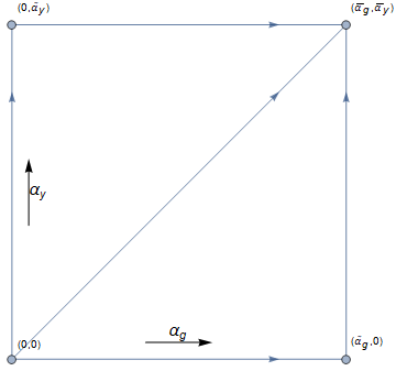
Refer to caption
Figure 16: Topology of the RG-flow between 4 fixed points.

Figure 17 shows the bifurcations of the sets of fixed points which were indicated as pairs 8 and 10 in the previous section. Here, we see the transcritical and saddle-node bifurcations that were found in the previous section. In addition, there is an extra transcritical bifurcation at the solid red line, where a non-trivial fixed point branches of. The solid red line converges to the branching point at x=5.5𝑥5.5x=5.5 that was found in the Veneziano limit. Furthermore, we see a transcritical bifurcation at non-trivial value of αysubscript𝛼𝑦\alpha_{y} (dash-dotted red line), where a non-trivial fixed point splits of. This transcritical bifurcation converges to the branching point found at x=11.6𝑥11.6x=11.6 in the Veneziano limit. The two non-trivial fixed points disappear through a saddle-node bifurcation at the solid blue line, which is related to the blue dashed line representing the saddle-node bifurcation that was found in the αy=0subscript𝛼𝑦0\alpha_{y}=0 space. The solid blue line converges to limit point that was found at x=5.5𝑥5.5x=5.5 in the Veneziano limit.

Figure 17 shows the bifurcations of the sets of fixed points which were indicated by the pairs 3 and 4 in the previous section. Here, we see the transcritical and saddle-node bifurcations that were found in the previous section. In addition, there is an extra transcritical bifurcation at the solid red line, where a non-trivial fixed point branches of. The solid red line converges to the branching point at x=5.5𝑥5.5x=5.5 that was found in the Veneziano limit. Furthermore, we see a trancritical bifurcation at non-trivial value of αysubscript𝛼𝑦\alpha_{y} (dash-dotted red line), where a non-trivial fixed point splits of. This transcritical bifurcation converges to the branching point found at x=11.6𝑥11.6x=11.6 in the Veneziano limit. The two non-trivial fixed points disappear through a saddle-node bifurcation at the solid blue line, which is related to the blue dashed line representing the saddle-node bifurcation that was found in the αy=0subscript𝛼𝑦0\alpha_{y}=0 space. The solid blue line converges to limit point that was found at x=5.5𝑥5.5x=5.5 in the Veneziano limit.

Figure 17 shows the bifurcations of the sets of fixed points which were indicated by the pairs 6 and 9 in the previous section. Here, we see the transcritical and saddle-node bifurcations that were found in the previous section. In addition there is an extra transcritical bifurcation at the solid red line, where a non-trivial fixed point branches of. The solid red line converges to the branching point at x=7.4𝑥7.4x=7.4 that was found in the Veneziano limit. Furthermore, we see a transcritical bifurcation at non-trivial value of αgsubscript𝛼𝑔\alpha_{g} (dash-dotted black line), where a non-trivial fixed point splits of. This transcritical bifurcation diverges in the Veneziano limit. The two non-trivial fixed points disappear through a saddle-node bifurcation at the solid blue line, which is related to the blue dashed line representing the saddle-node bifurcation that was found in the αy=0subscript𝛼𝑦0\alpha_{y}=0 space. The solid blue line intersects the black dash-dotted line at SNT6. Therefore only in a small interval Nc(1.2,1.5)subscript𝑁𝑐1.21.5N_{c}\in(1.2,1.5) the non-trivial fixed points disappear through a saddle-node bifurcation, while at larger Ncsubscript𝑁𝑐N_{c} the non-trivial fixed points that branch of from the solid red line and the black dash-dotted line diverge for small values of x𝑥x. In addition, for these fixed points we find a saddle-node bifurcation curve not only in the αy=0subscript𝛼𝑦0\alpha_{y}=0 space, as was the case in the previous figures, but also in the αg=0subscript𝛼𝑔0\alpha_{g}=0 space (dash-dotted blue line).

Figure 17 shows a few more transcritical bifurcation curves lying in the αgnt=0superscriptsubscript𝛼𝑔𝑛𝑡0\alpha_{g}^{nt}=0 and/or αynt=0superscriptsubscript𝛼𝑦𝑛𝑡0\alpha_{y}^{nt}=0 subspace. Non-trivial fixed points that are related to these transcritical bifurcation curves, all diverge in one or multiple couplings for small x𝑥x instead of disappearing through a saddle-node bifurcation. We notice the the black, solid red and dashed red line involve the sets of equilibria 1 and 2, as labeled in the previous section.
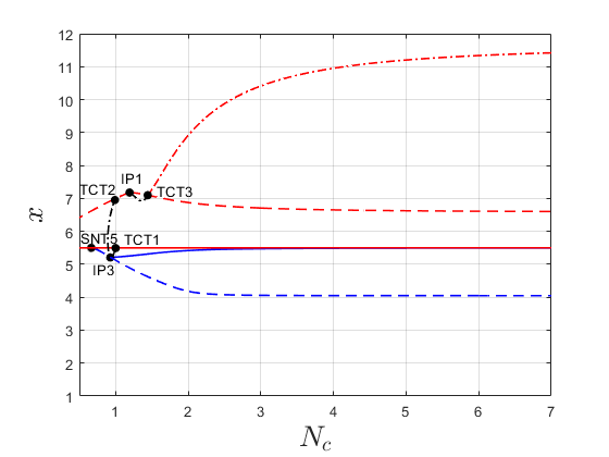
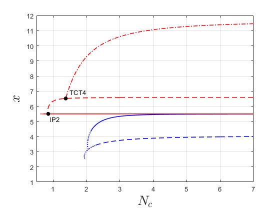
Refer to caption
(a)
Refer to caption
(b)
Refer to caption
(c)
Refer to caption
(d)
Refer to caption
Figure 17: Bifurcations in the RG-flow of (19) in the (Nc,x)subscript𝑁𝑐𝑥(N_{c},x)-plane. CP: Cusp bifurcation. SNT: Saddle-Node-Transcritical bifurcation. TCT: Transcritical-Transcritical bifurcation. IP: degenerate bifurcation point.

The eigenvectors that cross zero at the saddle-node bifurcations shown in Figure 17 and 17 are shown in Table 6 for Nc=3subscript𝑁𝑐3N_{c}=3 along with the eigenvalues of the other eigenvectors. We see that in this model the bifurcations are strongly triggered by the αgsubscript𝛼𝑔\alpha_{g} interaction. Furthermore, as in the previous, model we find two complex eigenvalues for the saddle-node bifurcation of point the non-trivial fixed points 3 and 4. Eigenvectors corresponding to the complex eigenvalues are directed along the four-fermion couplings, and have very small contributions (|ηαg|<0.004,|ηαy|<0.016formulae-sequencesubscript𝜂subscript𝛼𝑔0.004subscript𝜂subscript𝛼𝑦0.016|\eta_{\alpha_{g}}|<0.004,|\eta_{\alpha_{y}}|<0.016) along the eαgsubscript𝑒subscript𝛼𝑔e_{\alpha_{g}} and eαysubscript𝑒subscript𝛼𝑦e_{\alpha_{y}} direction, meaning that this complex scaling behavior involves operators, which are linear combinations of the effective four-fermi interactions.

Table 6: Eigenvalues and critical eigenvectors crossing marginality of the saddle-node bifurcation with non-trivial αg,αysubscript𝛼𝑔subscript𝛼𝑦\alpha_{g},\alpha_{y} at Nc=3subscript𝑁𝑐3N_{c}=3.
Equilibria (Nc,x)subscript𝑁𝑐𝑥(N_{c},x) Eigenvalues Critical eigenvector
8, 10 (3.00,5.47)3.005.47(3.00,5.47) {2.06,2.04,1.93,1.83,0.20,0}2.062.041.931.830.200\{-2.06,-2.04,-1.93,-1.83,-0.20,0\} (0.92,0.36,0.11,0.00,0.04, 0.07)0.920.360.110.000.040.07(0.92,0.36,0.11,0.00,-0.04,\;0.07)
3, 4 (3.00,5.34)3.005.34(3.00,5.34) {2.38±0.28i,2.34,1.36,1.09,0}plus-or-minus2.380.28𝑖2.341.361.090\{2.38\pm 0.28i,-2.34,-1.36,-1.09,0\} (0.69,0.29,0.32,0.09, 0.41,0.39)0.690.290.320.090.410.39(0.69,0.29,0.32,0.09,\;0.41,-0.39)

Furthermore, we find multiple bifurcation points in Figure 17, which are reported in Table 7. The first cusp bifurcation and the points SNT5, IP1 and IP2 were already found in the previous model. In addition, we find an extra cusp point in the saddle-node bifurcation curve in the αg=0subscript𝛼𝑔0\alpha_{g}=0 space. This curve has another cusp bifurcation at IP1, making IP1 even more degenerate. The points TCT1 up to TCT6 all describe the intersection of two transcritical bifurcation curves, and can be described by the normal form

{x˙=αx+x2,y˙=βy+y2.cases˙𝑥𝛼𝑥superscript𝑥2otherwise˙𝑦𝛽𝑦superscript𝑦2otherwise\begin{cases}\dot{x}=\alpha x+x^{2},\\ \dot{y}=\beta y+y^{2}.\end{cases} (23)

Finally, IP3 describes a point where 2 saddle-node bifurcation curves and 2 branches of a transcritical bifurcation intersect, and can therefore be described as a saddle-node-transcritical bifurcation, where an additional saddle-node bifurcation intersects. Four fixed points are involved in this bifurcation.

Table 7: Bifurcations found in the model of QCD4 (19) shown in Figure 17.
Bifurcation Ncsubscript𝑁𝑐N_{c} Nfsubscript𝑁𝑓N_{f} x𝑥x αgsubscript𝛼𝑔\alpha_{g} αysubscript𝛼𝑦\alpha_{y} gSsubscript𝑔𝑆g_{S} gVsubscript𝑔𝑉g_{V} gV1subscript𝑔subscript𝑉1g_{V_{1}} gV2subscript𝑔subscript𝑉2g_{V_{2}}
CP 1.621.621.62 9.829.829.82 6.076.076.07 0.050.050.05 00 0.030.030.03 0.170.17-0.17 0.010.010.01 0.220.220.22
CP 2.322.322.32 4.754.754.75 2.052.052.05 00 0.200.200.20 0.550.550.55 0.320.32-0.32 0.200.200.20 0.510.510.51
SNT5 0.660.660.66 3.653.653.65 5.505.505.50 00 00 00 00 00 00
SNT6 1.701.701.70 10.9510.9510.95 6.466.466.46 0.030.030.03 00 0.100.10-0.10 0.170.17-0.17 0.050.05-0.05 0.230.230.23
TCT1 1.001.001.00 5.505.505.50 5.505.505.50 00 00 00 00 00 00
TCT2 1.001.001.00 6.956.956.95 6.956.956.95 00 00 00 0.140.14-0.14 00 0.140.140.14
TCT3 1.441.441.44 10.2310.2310.23 7.107.107.10 00 00 0.130.130.13 0.150.15-0.15 0.070.070.07 0.200.200.20
TCT4 1.381.381.38 8.978.978.97 6.526.526.52 00 00 0.400.400.40 0.100.10-0.10 0.190.190.19 0.420.42-0.42
TCT5 1.391.391.39 10.0210.0210.02 7.197.197.19 00 00 0.100.10-0.10 0.160.16-0.16 0.050.05-0.05 0.200.200.20
TCT6 1.451.451.45 9.989.989.98 6.876.876.87 00 00 0.400.40-0.40 0.130.13-0.13 0.210.21-0.21 0.390.390.39
IP1 1.191.191.19 8.548.548.54 7.187.187.18 00 00 00 0.160.16-0.16 00 0.170.170.17
IP2 0.850.850.85 4.694.694.69 5.505.505.50 00 00 00 00 00 0.730.73-0.73
IP3 0.930.930.93 4.824.824.82 5.215.215.21 0.050.050.05 00 0.010.01-0.01 0.010.01-0.01 0.000.000.00 0.010.010.01

3.3 Discussion of the Results

In this section, we have seen how the addition of a scalar field alters the bifurcations found in the previous section. In particular, we would like to know whether we find similar behavior in the (αg>0,αy>0)formulae-sequencesubscript𝛼𝑔0subscript𝛼𝑦0(\alpha_{g}>0,\alpha_{y}>0) space as we found in the (αg>0(\alpha_{g}>0, αy=0)\alpha_{y}=0) space. We find the transcritical bifurcation at x=5.5𝑥5.5x=5.5, which marks the upper edge of the conformal window. This transcritical bifurcation now indicates the intersection of three fixed points: one on the (αg=0,αy=0)formulae-sequencesubscript𝛼𝑔0subscript𝛼𝑦0(\alpha_{g}=0,\alpha_{y}=0) subspace, one on the (αg>0,αy=0)formulae-sequencesubscript𝛼𝑔0subscript𝛼𝑦0(\alpha_{g}>0,\alpha_{y}=0) subspace, and one on the (αg>0,αy>0)formulae-sequencesubscript𝛼𝑔0subscript𝛼𝑦0(\alpha_{g}>0,\alpha_{y}>0). Furthermore, at this line there are two different transcritical bifurcation curves for different values of (gS,gV,gV1,gV2)subscript𝑔𝑆subscript𝑔𝑉subscript𝑔subscript𝑉1subscript𝑔subscript𝑉2(g_{S},g_{V},g_{V_{1}},g_{V_{2}}) as was also found in the previous model. One of these bifurcations is shown in Figure 17 and the other in Figure 17. We see that both saddle-node bifurcations that could indicate the lower edge of the conformal window in the model with αy=0subscript𝛼𝑦0\alpha_{y}=0 have a related saddle-node bifurcation in the (αg>0,αy>0)formulae-sequencesubscript𝛼𝑔0subscript𝛼𝑦0(\alpha_{g}>0,\alpha_{y}>0) space, indicating that the phase transition at the lower edge of the conformal window is similar to the previous section and involves the merger of fixed points, followed by a walking behavior of the coupling constant, that changes continuously to a running behavior. However, the non-trivial saddle-node bifurcations are found at a larger value of x𝑥x than the ones in the αy=0subscript𝛼𝑦0\alpha_{y}=0 subspace, and are triggered by the αgsubscript𝛼𝑔\alpha_{g} interaction instead of the gSsubscript𝑔𝑆g_{S} interaction. This curve is very close but slightly below x=5.5𝑥5.5x=5.5 at large values of Ncsubscript𝑁𝑐N_{c} and slightly decreases towards smaller Ncsubscript𝑁𝑐N_{c}. Therefore, the conformal window is much smaller in the theory that contains a scalar field in the adjoint representation, although fixed points and renormalized trajectories between those points remain to exist for smaller values of x𝑥x, but these are very unstable and require a large degree of fine-tuning within this model.

Furthermore, we find that the fixed points, which were labeled by 5 and 7 have no related fixed points with non-trivial value of αysubscript𝛼𝑦\alpha_{y}. Therefore, we do not have the spiraling behavior related to those fixed points as we had in the previous section. For the saddle-node bifurcation of the pair labeled by 6 and 9 there is only a related bifurcation with non-trivial and positive αgsubscript𝛼𝑔\alpha_{g} and αysubscript𝛼𝑦\alpha_{y} in a small interval Nc(1.2,1.5)subscript𝑁𝑐1.21.5N_{c}\in(1.2,1.5), which makes it irrelevant for the physical model, since we require integer values of Ncsubscript𝑁𝑐N_{c}. Therefore, we find that the non-trivial fixed points of the sets 1, 2, 6 and 9 all diverge for small x𝑥x.

4 Conclusions and Outlook

We have evaluated an effective model for QCD4, and studied the fixed points and their bifurcations in and close to the conformal window. We have found a fixed point merger (saddle-node bifurcation) in the Veneziano limit at Nf/Nc=4.049subscript𝑁𝑓subscript𝑁𝑐4.049N_{f}/N_{c}=4.049 indicating the lower edge of the conformal window. This prediction is similar to the ones by [3, 15], where the same model was analyzed. Furthermore, we have continued this bifurcation to the small Ncsubscript𝑁𝑐N_{c} regime, and found that this curve is more or less constant up to (Nc=3.00,Nf=12.17)formulae-sequencesubscript𝑁𝑐3.00subscript𝑁𝑓12.17(N_{c}=3.00,N_{f}=12.17). For Nc{1,2}subscript𝑁𝑐12N_{c}\in\{1,2\} the window is choked off. On the other hand, there exists another fixed point merger (corresponding to the same merger in the Veneziano limit), which is more or less constant up to (Nc=3.00,Nf=11.26)formulae-sequencesubscript𝑁𝑐3.00subscript𝑁𝑓11.26(N_{c}=3.00,N_{f}=11.26). For Nc=1subscript𝑁𝑐1N_{c}=1, these fixed points diverge instead of disappearing through a saddle-node bifurcation, while Nc=2subscript𝑁𝑐2N_{c}=2 is an intermediate value where they merger at large coupling constants. Both mergers could indicate the lower edge of the conformal window. In both cases the transition at the lower edge of the conformal window is an infinite order phase transition, generated by the effective scalar four-fermi interaction for Nc>2subscript𝑁𝑐2N_{c}>2. Furthermore, we have found a few extra sets of fixed points, that either disappear through saddle-node bifurcations or diverge.

The existence of multiple fixed points and multiple saddle-node bifurcations in this model, opens up many new questions about the lower edge of the conformal window. It might very well be the case that the infinite order perturbative beta function contains more fixed points apart from the well known Banks Zaks fixed point. This could result in a one or more transitions within the conformal window, where pairs of fixed points disappear through mergers. The lower edge is then reached when the last fixed point merger takes place. It would be interesting to try to relate such transitions to phase transitions that have been predicted in the quark gluon plasma. Furthermore, it would be interesting to extend the model with higher order effective interactions, and see which of the fixed points and saddle-node bifurcations remain to exist.

In this paper, we already extended the effective QCD model with an scalar field coupling through a Yukawa interaction to the fermions. This interaction turns out to destabilize the model. In this model we found that the 2 candidates for the conformal window both exist in this model as well. Although the lower edge of the conformal window is located at larger values of Nf/Ncsubscript𝑁𝑓subscript𝑁𝑐N_{f}/N_{c} for such a model, as was already predicted in [34]. The other fixed points on the other hand are pushed into a regime αg<0subscript𝛼𝑔0\alpha_{g}<0 and/or αy<0subscript𝛼𝑦0\alpha_{y}<0.

In addition, we have found that the model allows for complex scaling dimensions of the effective interactions. These complex scaling dimension contain both a scaling and a rotation of the associated operator. The rotation indicates that the (ir)relevant operators associated with the complex eigenvalue rotates in theory space, while the orbits move away from/towards the fixed point. Such behavour was early found for example in [36, 37]. For one pair of fixed points in the effective QCD model these complex scaling dimensions induced a clearly visible spiraling behavior in the RG-flow. This pair disappeared the the model extended with a scalar field and Yukawa coupling. It would be interesting to study these kind of exotic orbits in more detail, and maybe relate them to other exotic RG-flows that have been found, such as the bouncing solutions recently found in holographic studies [38]

Finally, we have shown that the use of bifurcation analysis in the study of RG-flows can be very useful tool in mapping out the fixed points and their transition in complicated model with multiple variables and parameters as was suggested in [3]. It would be interesting to use numerical tools such as the MATLAB package MatCont [1, 2] in other studies of renormalization group flows. In particular for non-perturbative beta functions this can lead to new insights. An alternative to our numerical approach would be to use Conley index theory and describe the exit sets for RG-flows as was suggested in [3].

Acknowledgements

It is a pleasure to thank Sergei Gukov for helpful discussions and comments on the manuscript. This work is partially supported by the Netherlands Organisation for Scientific Research (NWO) under the VIDI grant 680-47-518 and the Delta-Institute for Theoretical Physics (ΔΔ\Delta-ITP), both funded by the Dutch Ministry of Education, Culture and Science (OCW).

Appendix A Dynamical systems and bifurcation theory

A.1 Dynamical Systems

This appendix presents a short overview of relevant terminology from the field of dynamical systems, partially following [39]. A dynamical system is a tuple (T,X,Φt)𝑇𝑋superscriptΦ𝑡(T,X,\Phi^{t}), where X𝑋X is a state space, for time tT𝑡𝑇t\in T, Φt:XX:superscriptΦ𝑡𝑋𝑋\Phi^{t}:X\rightarrow X is a function defined on the state space, and typically T=0𝑇subscript0T=\mathbb{N}_{0} or T=𝑇T=\mathbb{N} for discrete dynamical systems, and T=0+𝑇superscriptsubscript0T=\mathbb{R}_{0}^{+} or T=𝑇T=\mathbb{R} for continuous dynamical systems. The collection of all maps {Φt}tTsubscriptsuperscriptΦ𝑡𝑡𝑇\{\Phi^{t}\}_{t\in T} is called the flow of the dynamical system and should satisfy

  • Φ0(x)=x;superscriptΦ0𝑥𝑥\Phi^{0}(x)=x;

  • Φs+t(x)=Φs(Φt(x)),xX,s,tTformulae-sequencesuperscriptΦ𝑠𝑡𝑥superscriptΦ𝑠superscriptΦ𝑡𝑥formulae-sequencefor-all𝑥𝑋𝑠𝑡𝑇\Phi^{s+t}(x)=\Phi^{s}(\Phi^{t}(x)),\,\forall x\in X,\,s,t\in T.

Therefore, the flow forms a group, if ΦΦ\Phi is invertible, and a semi-group otherwise.

For a point xX𝑥𝑋x\in X, one can define the orbit 𝒪Φ(x):={Φt(x)|tT)}\mathcal{O}_{\Phi}(x):=\{\Phi^{t}(x)|t\in T)\}. Furthermore, one can define the notion of an invariant set of a dynamical system.

Definition.

Given a dynamical system (T,X,Φt)𝑇𝑋superscriptΦ𝑡(T,X,\Phi^{t}),

  • a forward invariant set is a set UX𝑈𝑋U\subset X such that Φt(U)UsuperscriptΦ𝑡𝑈𝑈\Phi^{t}(U)\subseteq U t0;for-all𝑡0\forall t\geq 0;

  • a backward invariant set is a set UX𝑈𝑋U\subset X such that Φt(U)UsuperscriptΦ𝑡𝑈𝑈\Phi^{t}(U)\subseteq U t0;for-all𝑡0\forall t\leq 0;

  • a set that is both forward and backward invariant is called an invariant set of the dynamical system.

If the map ΦtsuperscriptΦ𝑡\Phi^{t} is non-invertible and T𝑇T is only defined on positive numbers, every forward invariant set is called an invariant set of the dynamical system. It is assumed above that Φt(x)superscriptΦ𝑡𝑥\Phi^{t}(x) is defined for all (t,x)T×X𝑡𝑥𝑇𝑋(t,x)\in T\times X. If it is not the case, i.e., given xX𝑥𝑋x\in X, Φt(x)superscriptΦ𝑡𝑥\Phi^{t}(x) is only defined for a subset of T𝑇T that includes t=0𝑡0t=0, the dynamical system is called local, and all definitions should be modified accordingly.

A natural way to generate a dynamical system is by a set of ordinary differential equations (continuous-time dynamical system) or a set of difference equations (discrete-time dynamical system). In this article, we consider dynamical systems generated by a set of differential equations, since those can be related to the beta functions of the renormalization group. Given the space X=n𝑋superscript𝑛X=\mathbb{R}^{n}, one can consider the system of autonomous ordinary differential equations

x˙=f(x),˙𝑥𝑓𝑥\dot{x}=f(x), (24)

where xn𝑥superscript𝑛x\in\mathbb{R}^{n} and f:nn:𝑓superscript𝑛superscript𝑛f:\mathbb{R}^{n}\rightarrow\mathbb{R}^{n}, which is assumed to be (sufficiently) smooth. If one defines the map Φt:nn:superscriptΦ𝑡superscript𝑛superscript𝑛\Phi^{t}:\mathbb{R}^{n}\rightarrow\mathbb{R}^{n} by Φt(x0)=x(t,x0)superscriptΦ𝑡subscript𝑥0𝑥𝑡subscript𝑥0\Phi^{t}(x_{0})=x(t,x_{0}), then the tuple (,n,Φ)superscript𝑛Φ(\mathbb{R},\mathbb{R}^{n},\Phi) is a (local) continuous-time dynamical system. The solutions for specified initial conditions, x(0,x0)=x0𝑥0subscript𝑥0subscript𝑥0x(0,x_{0})=x_{0}, define the orbits and the visualization of the flow is called the phase portrait. In the study of dynamical systems equilibria131313In this article, we often use the term fixed point instead of equilibrium to adapt to the terminology used in renormalization group theory, while in the terminology of dynamical systems the term fixed point is reserved for the discrete analogue of an equilibrium. and periodic, homoclinic, and heteroclinic orbits are of particular interest.

Definition.

Given a continuous-time dynamical system (,n,Φt)superscript𝑛superscriptΦ𝑡(\mathbb{R},\mathbb{R}^{n},\Phi^{t}), then a point xn𝑥superscript𝑛x\in\mathbb{R}^{n} is called an equilibrium if Φt(x)=xtsuperscriptΦ𝑡𝑥𝑥for-all𝑡\Phi^{t}(x)=x\;\forall t\in\mathbb{R}.

Definition.

Given a continuous-time dynamical system (,n,Φt)superscript𝑛superscriptΦ𝑡(\mathbb{R},\mathbb{R}^{n},\Phi^{t}), a point xn𝑥superscript𝑛x\in\mathbb{R}^{n}, and an orbit 𝒪Φ(x)subscript𝒪Φ𝑥\mathcal{O}_{\Phi}(x), then the orbit is called

  • a periodic orbit if x𝑥x is not an equilibrium and ΦT(y)=yy𝒪Φ(x)superscriptΦ𝑇𝑦𝑦for-all𝑦subscript𝒪Φ𝑥\Phi^{T}(y)=y\;\forall y\in\mathcal{O}_{\Phi}(x) for some T>0;𝑇0T>0; minimal such T𝑇T is called the period;

  • a homoclinic orbit if limtΦt(x)=limtΦt(x)=ysubscript𝑡superscriptΦ𝑡𝑥subscript𝑡superscriptΦ𝑡𝑥𝑦\lim_{t\rightarrow-\infty}\Phi^{t}(x)=\lim_{t\rightarrow\infty}\Phi^{t}(x)=y and Φt(x)ytsuperscriptΦ𝑡𝑥𝑦for-all𝑡\Phi^{t}(x)\neq y\;\forall t\in\mathbb{R}, where y𝑦y is an equilibrium;

  • a heteroclinic orbit if limtΦt(x)=yz=limtΦt(x)subscript𝑡superscriptΦ𝑡𝑥𝑦𝑧subscript𝑡superscriptΦ𝑡𝑥\lim_{t\rightarrow-\infty}\Phi^{t}(x)=y\neq z=\lim_{t\rightarrow\infty}\Phi^{t}(x), where y,z𝑦𝑧y,z are equilibria.

The topology of the phase portrait is characterized by its invariant sets and their stability. An invariant set is asymptotically stable, if all orbits starting in a neighborhood of the invariant set stay in this neighborhood and converge towards the invariant set if t𝑡t\rightarrow\infty and unstable otherwise. For generic equilibria the stability is determined by the eigenvalues of Jacobian matrix at the equilibrium. At the equilibrium, one can define the notions of a stable, unstable and critical eigenspace.

Definition.

Given a continuous-time dynamical system defined by equation (24)24(\ref{IntroBifAna:system}), with an equilibrium point at x0nsubscript𝑥0superscript𝑛x_{0}\in\mathbb{R}^{n}. Let A𝐴A be the Jacobian matrix of f𝑓f at x0subscript𝑥0x_{0}, (λ1,λ2,,λn)subscript𝜆1subscript𝜆2subscript𝜆𝑛(\lambda_{1},\lambda_{2},...,\lambda_{n}) its eigenvalues and η1,η2,,ηnsubscript𝜂1subscript𝜂2subscript𝜂𝑛\eta_{1},\eta_{2},...,\eta_{n} the corresponding (((generalized))) eigenvectors. Then

  • the stable eigenspace is given by Ts=span{η1,η2,,ηn};superscript𝑇𝑠spansuperscriptsubscript𝜂1superscriptsubscript𝜂2superscriptsubscript𝜂subscript𝑛T^{s}=\mathrm{span}\{\eta_{1}^{-},\eta_{2}^{-},...,\eta_{n_{-}}^{-}\};

  • the unstable eigenspace by Tu=span{η1+,η2+,,ηn++}superscript𝑇𝑢spansuperscriptsubscript𝜂1superscriptsubscript𝜂2superscriptsubscript𝜂subscript𝑛T^{u}=\mathrm{span}\{\eta_{1}^{+},\eta_{2}^{+},...,\eta_{n_{+}}^{+}\}, and

  • the critical eigenspace by Tc=span{η1c,η2c,,ηncc}superscript𝑇𝑐spansuperscriptsubscript𝜂1𝑐superscriptsubscript𝜂2𝑐superscriptsubscript𝜂subscript𝑛𝑐𝑐T^{c}=\mathrm{span}\{\eta_{1}^{c},\eta_{2}^{c},...,\eta_{n_{c}}^{c}\},

where ηi+superscriptsubscript𝜂𝑖\eta_{i}^{+} label (((generalized))) eigenvectors that correspond to eigenvalues λi+superscriptsubscript𝜆𝑖\lambda_{i}^{+} with positive real part, ηisuperscriptsubscript𝜂𝑖\eta_{i}^{-} (((generalized))) eigenvectors corresponding to eigenvalues λisuperscriptsubscript𝜆𝑖\lambda_{i}^{-} with negative real part and ηicsuperscriptsubscript𝜂𝑖𝑐\eta_{i}^{c} (((generalized))) eigenvectors corresponding to eigenvalues λicsuperscriptsubscript𝜆𝑖𝑐\lambda_{i}^{c} with zero real part. Furthermore, n++n+nc=nsubscript𝑛subscript𝑛subscript𝑛𝑐𝑛n_{+}+n_{-}+n_{c}=n.

An equilibrium is called hyperbolic if dim(Tc)=0dimensionsuperscript𝑇𝑐0\dim(T^{c})=0, stable if dim(Ts)=ndimensionsuperscript𝑇𝑠𝑛\dim(T^{s})=n and unstable if dim(Tu)1dimensionsuperscript𝑇𝑢1\dim(T^{u})\geq 1. Furthermore, an equilibrium with dim(Ts)=ndimensionsuperscript𝑇𝑠𝑛\dim(T^{s})=n or dim(Tu)=ndimensionsuperscript𝑇𝑢𝑛\dim(T^{u})=n is a node and an equilibrium with dim(Ts)1dimensionsuperscript𝑇𝑠1\dim(T^{s})\geq 1 and dim(Tu)1dimensionsuperscript𝑇𝑢1\dim(T^{u})\geq 1 is a saddle. The classification of non-hyperbolic equilibria not satisfying these conditions is more involved, and won’t be discussed further in this article. For a generic equilibrium in a continuous-time dynamical system, one can also define the notions of a stable and unstable manifold of the equilibrium.

Definition.

Given a continuous-time dynamical system (,X,Φt)𝑋superscriptΦ𝑡(\mathbb{R},X,\Phi^{t}), and an equilibrium point xX𝑥𝑋x\in X of ΦΦ\Phi, then

  • the stable manifold of x𝑥x is defined as Ws(Φ,x)={yX:limtΦt(y)=x}superscript𝑊𝑠Φ𝑥conditional-set𝑦𝑋subscript𝑡superscriptΦ𝑡𝑦𝑥W^{s}(\Phi,x)=\{y\in X:\lim_{t\rightarrow\infty}\Phi^{t}(y)=x\}, and

  • the unstable manifold as Wu(Φ,x)={yX:limtΦt(y)=x}superscript𝑊𝑢Φ𝑥conditional-set𝑦𝑋subscript𝑡superscriptΦ𝑡𝑦𝑥W^{u}(\Phi,x)=\{y\in X:\lim_{t\rightarrow-\infty}\Phi^{t}(y)=x\}.

For a dynamical system defined by (24), the stable manifold is at the equilibrium tangent to the stable eigenspace, while the unstable manifold is at the equilibrium tangent to the unstable eigenspace. For nonhyperbolic equilibria, one can introduce the concept of a center manifold Wlocc(Φ,x)superscriptsubscript𝑊loc𝑐Φ𝑥W_{\textrm{loc}}^{c}(\Phi,x), which is ncsubscript𝑛𝑐n_{c}-dimensional and tangent to the critical eigenspace at the equilibrium. The existence of this locally defined manifold is implied by the Center Manifold Theorem.

A.2 Bifurcation Analysis

A continuous-time dynamical system defined by a set of ordinary differential equations can be analyzed by solving the ODE’s numerically. However, if the differential equations also depend on a set of parameters, fα(x)subscript𝑓𝛼𝑥f_{\alpha}(x), αm𝛼superscript𝑚\alpha\in\mathbb{R}^{m}, one is often not interested in the exact solutions for specific values of α𝛼\alpha, but in the topological properties of the phase portrait such as the number of equilibria, limit cycles and their stability or the existence of homo- and heteroclinic orbits and chaotic attractors. In general, changes of the phase portrait, when α𝛼\alpha is varied, occur smoothly except for some specific values of α𝛼\alpha, where the topology of the phase portrait changes. Changes in the topology of the phase portrait are called bifurcations. Topology changes often occur near or within invariant sets. Bifurcations can be divided in 2 subclasses:

  • local bifurcations: bifurcations that can be detected by considering small but non-shrinking neighborhoods of equilibria or limit cycles.

  • global bifurcations: bifurcations that cannot be detected in this way. Topology changes typically involve multiple invariant sets.

In addition, bifurcations may be called subcritical or supercritical, depending on the stability of the equilibria or limit cycles that appear or disappear at the bifurcation. Furthermore, bifurcations can be characterized by their codimension. The codimension of a bifurcation in a generic system is given by the number of independent conditions that have to be satisfied for a bifurcation to happen, and for local bifurcations is often related to the number of critical eigenvalues of the Jacobian matrix at the equilibrium. Consequently, the codimension of a bifurcation is always smaller or equal to the dimension of the parameter space. In general, many types of bifurcations can be found. For an overview of possible bifurcations and their conditions, we refer to [40]. In this appendix, we discuss bifurcations and related terminology that is relevant for this article. In doing so, we closely follow [40]. Bifurcations in low dimensional systems and with low codimension can often be found using analytical techniques, but for higher dimensional systems and in particular for higher codimension of the bifurcation one often has to rely on numerical techniques. Several computer programs have been developed for bifurcation analysis. In this article we make use of the Matlab package Matcont [1, 2]. Bifurcation software relies on the conditions that have to be satisfied in order for a bifurcation to happen.

In different dynamical systems one can expect different bifurcations, which are not immediately defined by the same conditions. However, one would like to have a way of categorizing bifurcation in various systems. For this, we need the notion of topological equivalence. Consider two continuous-time dynamical systems:

x˙˙𝑥\displaystyle\dot{x} =f(x,α),xn,αm;formulae-sequenceabsent𝑓𝑥𝛼formulae-sequence𝑥superscript𝑛𝛼superscript𝑚\displaystyle=f(x,\alpha),\quad x\in\mathbb{R}^{n},\;\alpha\in\mathbb{R}^{m}; (25)
y˙˙𝑦\displaystyle\dot{y} =g(y,β),yn,βm.formulae-sequenceabsent𝑔𝑦𝛽formulae-sequence𝑦superscript𝑛𝛽superscript𝑚\displaystyle=g(y,\beta),\quad y\in\mathbb{R}^{n},\;\beta\in\mathbb{R}^{m}. (26)
Definition.

Dynamical systems (25)25(\ref{Intro:dynsys1}) and (26)26(\ref{Intro:dynsys2}) are topologically equivalent if

  • there exists a homeomorphism of the parameter space p:mm:𝑝superscript𝑚superscript𝑚p:\mathbb{R}^{m}\rightarrow\mathbb{R}^{m} s.t. β=p(α);𝛽𝑝𝛼\beta=p(\alpha);

  • there exists a parameter-dependent homeomorphism of the phase space hα:nn:subscript𝛼superscript𝑛superscript𝑛h_{\alpha}:\mathbb{R}^{n}\rightarrow\mathbb{R}^{n} s.t. y=hα(x)𝑦subscript𝛼𝑥y=h_{\alpha}(x), mapping orbits of the system (25)25(\ref{Intro:dynsys1}) at parameter values α𝛼\alpha onto orbits of the system (26)26(\ref{Intro:dynsys2}) at parameter values β=p(α)𝛽𝑝𝛼\beta=p(\alpha), preserving the direction of time.

Since many bifurcations are locally defined, one is often only interested in local topological equivalence near specific points.

Definition.

Dynamical systems (25)25(\ref{Intro:dynsys1}) and (26)26(\ref{Intro:dynsys2}) are locally topologically equivalent near the origin, if there exists a map (x,α)(hα(x),p(α))maps-to𝑥𝛼subscript𝛼𝑥𝑝𝛼(x,\alpha)\mapsto(h_{\alpha}(x),p(\alpha)), defined in a small neighborhood of (x,α)=(0,0)n×m𝑥𝛼00superscript𝑛superscript𝑚(x,\alpha)=(0,0)\in\mathbb{R}^{n}\times\mathbb{R}^{m} such that

  • p:mm:𝑝superscript𝑚superscript𝑚p:\mathbb{R}^{m}\rightarrow\mathbb{R}^{m} is a homeomorphism defined in a small neighbourhood of α=0𝛼0\alpha=0, p(0)=0;𝑝00p(0)=0;

  • hα:nn:subscript𝛼superscript𝑛superscript𝑛h_{\alpha}:\mathbb{R}^{n}\rightarrow\mathbb{R}^{n} is a parameter-dependent homeomorphism defined in a small neighborhood U𝑈U of x=0𝑥0x=0, h0(0)=0subscript000h_{0}(0)=0, and mapping orbits of the system (25)25(\ref{Intro:dynsys1}) in U𝑈U onto orbits of the system (26)26(\ref{Intro:dynsys2}) in hα(U)subscript𝛼𝑈h_{\alpha}(U), preserving the direction of time.

By coordinate translations one can easily generalize this definition to local topological equivalence near arbitrary points. Having these definitions, one can categorize bifurcations by topological equivalence to normal forms. Consider a polynomial continuous-time dynamical system

z˙=g(z,β;σ),zn,βk,σl,formulae-sequence˙𝑧𝑔𝑧𝛽𝜎formulae-sequence𝑧superscript𝑛formulae-sequence𝛽superscript𝑘𝜎superscript𝑙\dot{z}=g(z,\beta;\sigma),\quad z\in\mathbb{R}^{n},\,\beta\in\mathbb{R}^{k},\,\sigma\in\mathbb{R}^{l}, (27)

which has an equilibrium z=0𝑧0z=0 at β=0𝛽0\beta=0, satisfying k𝑘k bifurcation conditions. Here, σ𝜎\sigma is a vector of the coefficients of the polynomial g(z,β;σ)𝑔𝑧𝛽𝜎g(z,\beta;\sigma).

Definition.

System (27)27(\ref{Intro:dynsys3}) is a topological normal form for the bifurcation if any generic system (25)25(\ref{Intro:dynsys1}) with equilibrium x0subscript𝑥0x_{0} satisfying the bifurcation conditions α0subscript𝛼0\alpha_{0} is locally topologically equivalent near (x0,α0)subscript𝑥0subscript𝛼0(x_{0},\alpha_{0}) to (27)27(\ref{Intro:dynsys3}) for some values of the coefficients σisubscript𝜎𝑖\sigma_{i}.

We notice that the system (25) can have higher dimension than is needed for the bifurcation to occur: xn𝑥superscript𝑛x\in\mathbb{R}^{n}, while the normal form has zcncsuperscript𝑧𝑐superscriptsubscript𝑛𝑐z^{c}\in\mathbb{R}^{n_{c}} with nc<nsubscript𝑛𝑐𝑛n_{c}<n. In such a case, there is a continuation of the critical center manifold. For nearby parameter values (25) is locally topologically equivalent to

z˙csuperscript˙𝑧𝑐\displaystyle\dot{z}^{c} =g(zc,β;σ),absent𝑔superscript𝑧𝑐𝛽𝜎\displaystyle=g(z^{c},\beta;\sigma), (28)
z˙ssuperscript˙𝑧𝑠\displaystyle\dot{z}^{s} =zs,absentsuperscript𝑧𝑠\displaystyle=-z^{s}, (29)
z˙usuperscript˙𝑧𝑢\displaystyle\dot{z}^{u} =+zu,absentsuperscript𝑧𝑢\displaystyle=+z^{u}, (30)

where g(zc,β;σ)𝑔superscript𝑧𝑐𝛽𝜎g(z^{c},\beta;\sigma) is a normal form on the center manifold and zsns,zunuformulae-sequencesuperscript𝑧𝑠superscriptsubscript𝑛𝑠superscript𝑧𝑢superscriptsubscript𝑛𝑢z^{s}\in\mathbb{R}^{n_{s}},z^{u}\in\mathbb{R}^{n_{u}} correspond to the stable and unstable eigenspaces.

We now give a short discussion of local bifurcations which are encountered throughout the article. We begin with bifurcations in scalar one-parameter ODEs

x˙=f(x,α),x,α.formulae-sequence˙𝑥𝑓𝑥𝛼formulae-sequence𝑥𝛼\dot{x}=f(x,\alpha),\quad x\in\mathbb{R},\alpha\in\mathbb{R}. (31)

In the n𝑛n-dimensional case, each normal form below is the normal form (28) on the one-dimensional center manifold.

Saddle-Node Bifurcation

This bifurcation is a codimension one bifurcation at which two equilibria collide and disappear, and is also known as fold or limit point bifurcation. The bifurcation occurs at (x¯,α¯)¯𝑥¯𝛼(\bar{x},\bar{\alpha}), if the following conditions hold for the system (31):

  • f(x¯,α¯)=0,𝑓¯𝑥¯𝛼0f(\bar{x},\bar{\alpha})=0,

  • fx(x¯,α¯)=0subscript𝑓𝑥¯𝑥¯𝛼0f_{x}(\bar{x},\bar{\alpha})=0,

  • a=12fxx(x¯,α¯)0𝑎12subscript𝑓𝑥𝑥¯𝑥¯𝛼0a=\frac{1}{2}f_{xx}(\bar{x},\bar{\alpha})\neq 0,

  • fα(x¯,α¯)0subscript𝑓𝛼¯𝑥¯𝛼0f_{\alpha}(\bar{x},\bar{\alpha})\neq 0,

where a𝑎a is the quadratic coefficient of the system (31). The system is then locally topologically equivalent near (x¯,α¯)¯𝑥¯𝛼(\bar{x},\bar{\alpha}) to the normal form

y˙=β±y2,y,βformulae-sequence˙𝑦plus-or-minus𝛽superscript𝑦2𝑦𝛽\dot{y}=\beta\pm y^{2},\quad y,\beta\in\mathbb{R} (32)

near (y,β)=(0,0)𝑦𝛽00(y,\beta)=(0,0) (see Figure 18).

Refer to caption
Figure 18: Saddle-Node bifurcation in the system y˙=βy2˙𝑦𝛽superscript𝑦2\dot{y}=\beta-y^{2}.

Transcritical Bifurcation

This bifurcation is a codimension one bifurcation in the class of systems that always have a trivial equilibrium, and is also a branching point: At the bifurcation, two equilibria collide and exchange their stability. The bifurcation occurs at (x¯,α¯)¯𝑥¯𝛼(\bar{x},\bar{\alpha}), if the following conditions hold for the system (31):

  • f(x¯,α¯)=0𝑓¯𝑥¯𝛼0f(\bar{x},\bar{\alpha})=0,

  • fx(x¯,α¯)=fα(x¯,α¯)=0subscript𝑓𝑥¯𝑥¯𝛼subscript𝑓𝛼¯𝑥¯𝛼0f_{x}(\bar{x},\bar{\alpha})=f_{\alpha}(\bar{x},\bar{\alpha})=0,

  • fxx(x¯,α¯)0subscript𝑓𝑥𝑥¯𝑥¯𝛼0f_{xx}(\bar{x},\bar{\alpha})\neq 0,

  • fxα(x¯,α¯)0subscript𝑓𝑥𝛼¯𝑥¯𝛼0f_{x\alpha}(\bar{x},\bar{\alpha})\neq 0.

The system is then locally topologically equivalent near (x¯,α¯)¯𝑥¯𝛼(\bar{x},\bar{\alpha}) to the normal form

y˙=βy±y2,y,βformulae-sequence˙𝑦plus-or-minus𝛽𝑦superscript𝑦2𝑦𝛽\dot{y}=\beta y\pm y^{2},\quad y,\beta\in\mathbb{R} (33)

near (y,β)=(0,0)𝑦𝛽00(y,\beta)=(0,0) (see Figure 19).

Refer to caption
Figure 19: Transcritical bifurcation in the system y˙=βyy2˙𝑦𝛽𝑦superscript𝑦2\dot{y}=\beta y-y^{2}.

Notice that we can transform the normal form of the tanscritical bifurcation to the normal form of the saddle-node bifurcation by the non-invertible coordinate transformation

(y,β)(y±β2,β24).maps-to𝑦𝛽plus-or-minus𝑦𝛽2minus-or-plussuperscript𝛽24(y,\beta)\mapsto\left(y\pm\frac{\beta}{2},\mp\frac{\beta^{2}}{4}\right).

This is called a nonversal unfolding of the saddle-node bifurcation.

Pitchfork Bifurcation

This bifurcation is a codimension one bifurcation for systems with reflectional symmetry, and is also a branching point: At the bifurcation one equilibrium splits into three equilibria. The bifurcation occurs at (x¯,α¯)¯𝑥¯𝛼(\bar{x},\bar{\alpha}), if the following conditions hold for the system (31):

  • f(x¯,α¯)=0𝑓¯𝑥¯𝛼0f(\bar{x},\bar{\alpha})=0

  • fx(x¯,α¯)=fxx(x¯,α¯)=fα(x¯,α¯)=0subscript𝑓𝑥¯𝑥¯𝛼subscript𝑓𝑥𝑥¯𝑥¯𝛼subscript𝑓𝛼¯𝑥¯𝛼0f_{x}(\bar{x},\bar{\alpha})=f_{xx}(\bar{x},\bar{\alpha})=f_{\alpha}(\bar{x},\bar{\alpha})=0,

  • fxxx(x¯,α¯)0subscript𝑓𝑥𝑥𝑥¯𝑥¯𝛼0f_{xxx}(\bar{x},\bar{\alpha})\neq 0,

  • fxα(x¯,α¯)0subscript𝑓𝑥𝛼¯𝑥¯𝛼0f_{x\alpha}(\bar{x},\bar{\alpha})\neq 0.

The system is then locally topologically equivalent near (x¯,α¯)¯𝑥¯𝛼(\bar{x},\bar{\alpha}) to the normal form

y˙=βy±y3,y,βformulae-sequence˙𝑦plus-or-minus𝛽𝑦superscript𝑦3𝑦𝛽\dot{y}=\beta y\pm{y}^{3},\quad y,\beta\in\mathbb{R} (34)

near (y,β)=(0,0)𝑦𝛽00(y,\beta)=(0,0) (see Figure 20). The - sign gives the supercritical case where a stable equilibrium splits into two stable equilibria and an unstable equilibrium, and the ++ sign is the subcritical case, where an unstable equilibrium splits into two unstable equilibria and a stable equilibrium.
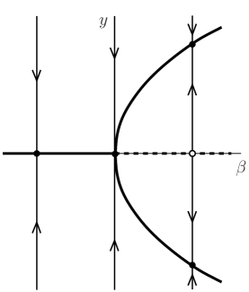
Refer to caption
Figure 20: Supercritical pitchfork bifurcation in the system y˙=βyy3˙𝑦𝛽𝑦superscript𝑦3\dot{y}=\beta y-y^{3}.

We continue with two bifurcations in scalar two-parameter ODEs

x˙=f(x,α),x,α=(α1,α2)2.formulae-sequence˙𝑥𝑓𝑥𝛼formulae-sequence𝑥𝛼subscript𝛼1subscript𝛼2superscript2\dot{x}=f(x,\alpha),\quad x\in\mathbb{R},\ \alpha=(\alpha_{1},\alpha_{2})\in\mathbb{R}^{2}. (35)

In the n𝑛n-dimensional case, each normal form below is the normal form (28) on the corresponding one-dimensional center manifold.

Cusp Bifurcation

This bifurcation is a codimension two bifurcation in generic systems, where two branches of saddle-node bifurcation meet tangentially. Nearby, the system can have three equilibria which collide and disappear at the saddle-node bifurcations. The bifurcation occurs at (x¯,α¯)¯𝑥¯𝛼(\bar{x},\bar{\alpha}), if the following conditions hold for the system (35):

  • f(x¯,α¯)=0𝑓¯𝑥¯𝛼0f(\bar{x},\bar{\alpha})=0,

  • fx(x¯,α¯)=fxx(x¯,α¯)=0subscript𝑓𝑥¯𝑥¯𝛼subscript𝑓𝑥𝑥¯𝑥¯𝛼0f_{x}(\bar{x},\bar{\alpha})=f_{xx}(\bar{x},\bar{\alpha})=0,

  • c=16fxxx(x¯,α¯)0𝑐16subscript𝑓𝑥𝑥𝑥¯𝑥¯𝛼0c=\frac{1}{6}f_{xxx}(\bar{x},\bar{\alpha})\neq 0,

  • the map (x,α)(f(x,α),fx(x,α),fxx(x,α))maps-to𝑥𝛼𝑓𝑥𝛼subscript𝑓𝑥𝑥𝛼subscript𝑓𝑥𝑥𝑥𝛼(x,\alpha)\mapsto(f(x,\alpha),f_{x}(x,\alpha),f_{xx}(x,\alpha)) is regular at (x,α)=(x¯,α¯)𝑥𝛼¯𝑥¯𝛼(x,\alpha)=(\bar{x},\bar{\alpha}),

where c𝑐c is the cubic coefficient of the system (35). The system is then locally topologically equivalent near (x¯,α¯)¯𝑥¯𝛼(\bar{x},\bar{\alpha}) to the normal form

y˙=β1+β2y±y3,y,β,β2formulae-sequence˙𝑦plus-or-minussubscript𝛽1subscript𝛽2𝑦superscript𝑦3𝑦subscript𝛽,subscript𝛽2\dot{y}=\beta_{1}+\beta_{2}y\pm y^{3},\quad y,\beta_{,}\beta_{2}\in\mathbb{R} (36)

near (y,β)=(0,0)𝑦𝛽00(y,\beta)=(0,0) (see Figure 21).

Refer to caption
Figure 21: Cusp bifurcation in the system y˙=β1+β2yy3˙𝑦subscript𝛽1subscript𝛽2𝑦superscript𝑦3\dot{y}=\beta_{1}+\beta_{2}y-y^{3}.

Saddle-Node-Transcritical Bifurcation

This bifurcation is a codimension two bifurcation in the class of systems that always have a trivial equilibrium, where two branches of a transcritical bifurcation curve meet on a saddle-node bifurcation curve. There exist two types of this bifurcation. One can be seen as a nonversal unfolding of a Cusp bifurcation, while the other can be obtained as an unfolding of a degenerate Bogdanov-Takens bifurcation. Here, we discuss only the first case.
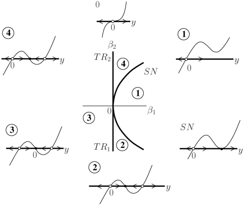
Refer to caption
Figure 22: Saddle-node-transcritical bifurcation in the system y˙=β1y+β2y2+y3˙𝑦subscript𝛽1𝑦subscript𝛽2superscript𝑦2superscript𝑦3\dot{y}=\beta_{1}y+\beta_{2}y^{2}+y^{3}.

Nearby, the system can have three equilibria: One pair has a transcritical bifurcation at one of the branches and another pair has a transcritical bifurcation at another branch. The last possible pair of equilibria collides and disappears at the saddle-node bifurcation curve. If the bifurcation occurs at (x¯,α¯)¯𝑥¯𝛼(\bar{x},\bar{\alpha}), then the system (35) is locally topologically equivalent near (x¯,α¯)¯𝑥¯𝛼(\bar{x},\bar{\alpha}) to the normal form given by

y˙=β1y+β2y2±y3,y,β1,β2formulae-sequence˙𝑦plus-or-minussubscript𝛽1𝑦subscript𝛽2superscript𝑦2superscript𝑦3𝑦subscript𝛽1subscript𝛽2\dot{y}=\beta_{1}y+\beta_{2}y^{2}\pm y^{3},\quad y,\beta_{1},\beta_{2}\in\mathbb{R} (37)

near (y,β)=(0,0)𝑦𝛽00(y,\beta)=(0,0) (see Figure 22). We then find a transcritical bifurcation along the line β1=0subscript𝛽10\beta_{1}=0, and a saddle-node bifurcation along β1=±β224subscript𝛽1plus-or-minussuperscriptsubscript𝛽224\beta_{1}=\pm\frac{\beta_{2}^{2}}{4}. The normal form can be transformed to the normal form of the cusp bifurcation through the transformation

(y,β1,β2)(y±β23,2β2327β1β23,β1β223).maps-to𝑦subscript𝛽1subscript𝛽2plus-or-minus𝑦subscript𝛽23minus-or-plus2superscriptsubscript𝛽2327subscript𝛽1subscript𝛽23minus-or-plussubscript𝛽1superscriptsubscript𝛽223(y,\beta_{1},\beta_{2})\mapsto\left(y\pm\frac{\beta_{2}}{3},\frac{2\beta_{2}^{3}}{27}\mp\frac{\beta_{1}\beta_{2}}{3},\beta_{1}\mp\frac{\beta_{2}^{2}}{3}\right).

Finally, we discuss for completeness the last codimension one local bifurcation in generic ODEs (25), i.e. Andronov-Hopf bifurcation. Note that it does not occur in our RG-flows but might appear in other models. For this bifurcation, the center manifold is two-dimensional, so it is sufficient to consider (25) with n=2𝑛2n=2 and m=1𝑚1m=1.

Andronov-Hopf Bifurcation

This bifurcation is a codimension one bifurcation, and implies the birth of a periodic orbit (limit cycle). The bifurcation occurs at an equilibrium (x¯,α¯)¯𝑥¯𝛼(\bar{x},\bar{\alpha}), if a pair of two conjugate complex eigenvalues of the Jacobian matrix crosses the imaginary axis. Generically, at the bifurcation the system is locally topologically equivalent near (x¯,α¯)¯𝑥¯𝛼(\bar{x},\bar{\alpha}) to the normal form

y˙1subscript˙𝑦1\displaystyle\dot{y}_{1} =\displaystyle= βy1y2±y1(y12+y22),plus-or-minus𝛽subscript𝑦1subscript𝑦2subscript𝑦1superscriptsubscript𝑦12superscriptsubscript𝑦22\displaystyle\beta y_{1}-y_{2}\pm y_{1}\left(y_{1}^{2}+y_{2}^{2}\right),
y˙2subscript˙𝑦2\displaystyle\dot{y}_{2} =\displaystyle= y1+βy2±y2(y12+y22),plus-or-minussubscript𝑦1𝛽subscript𝑦2subscript𝑦2superscriptsubscript𝑦12superscriptsubscript𝑦22\displaystyle y_{1}+\beta y_{2}\pm y_{2}\left(y_{1}^{2}+y_{2}^{2}\right),

near (y1,y2,β)=(0,0,0)subscript𝑦1subscript𝑦2𝛽000(y_{1},y_{2},\beta)=(0,0,0). The plus sign corresponds to the subcritical case, where an unstable limit cycles is created and the minus sign to the supercritical case, where a stable limit cycle is created (see Figure 23).
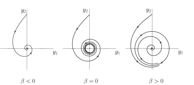
Refer to caption
Figure 23: Supercritical Andronov-Hopf bifurcation in the system y˙1=βy1y2y1(y12+y22),y˙2=y1+βy2y2(y12+y22).formulae-sequencesubscript˙𝑦1𝛽subscript𝑦1subscript𝑦2subscript𝑦1superscriptsubscript𝑦12superscriptsubscript𝑦22subscript˙𝑦2subscript𝑦1𝛽subscript𝑦2subscript𝑦2superscriptsubscript𝑦12superscriptsubscript𝑦22\dot{y}_{1}=\beta y_{1}-y_{2}-y_{1}\left(y_{1}^{2}+y_{2}^{2}\right),\ \dot{y}_{2}=y_{1}+\beta y_{2}-y_{2}\left(y_{1}^{2}+y_{2}^{2}\right).

Appendix B Beta functions in QCD4

B.1 Feynman Rules for QCD4 with a Four-Fermi Interaction

The theory as discussed in section 2 has three propagators:141414All Feynman diagrams are generated with the Tikz-Feynman package [41].

[Uncaptioned image]

where μ,ν𝜇𝜈\mu,\nu label the space-time indices, A,B𝐴𝐵A,B label the colors in the adjoint representation of SU(Nc)𝑆𝑈subscript𝑁𝑐SU(N_{c}), a,b𝑎𝑏a,b label the color in the fundamental representation of SU(Nc)𝑆𝑈subscript𝑁𝑐SU(N_{c}) and {i,j}𝑖𝑗\{i,j\} label the flavor in the fundamental representation of SU(Nf)𝑆𝑈subscript𝑁𝑓SU(N_{f}). Furthermore, we take the Landau gauge in which the gauge parameter ξ=0𝜉0\xi=0.

The fermion-gluon interaction (gauge vertex) is given by:

[Uncaptioned image]

Furthermore, there are four four-fermi interactions:

[Uncaptioned image]

Notice that the vertices have been split up in two parts. This is done to make clear along which lines the color charge is conserved, and will make the calculations in appendix B.3 more tractable, but has no further physical meaning.

B.2 Beta Function for the Gauge Vertex

In this appendix, we reproduce the method used in [15] to calculate the beta function for the gauge vertex. We’re only interested in gauge invariant contributions to the beta function, but the Wetterich equation does not necessarily respect gauge invariance. Therefore, we do not use the exact renormalization approach. Instead we start from the well known 2-loop perturbative beta function for QCD4 with Ncsubscript𝑁𝑐N_{c} colors and Nfsubscript𝑁𝑓N_{f} massless flavors [5]:

βg[2]ΛdαgdΛ=2b0αg22b1αg3superscriptsubscript𝛽𝑔delimited-[]2Λ𝑑subscript𝛼𝑔𝑑Λ2subscript𝑏0superscriptsubscript𝛼𝑔22subscript𝑏1superscriptsubscript𝛼𝑔3\beta_{g}^{[2]}\equiv\Lambda\frac{d\alpha_{g}}{d\Lambda}=-2b_{0}\alpha_{g}^{2}-2b_{1}\alpha_{g}^{3} (38)

with

b0subscript𝑏0\displaystyle b_{0} =113Nc23Nfabsent113subscript𝑁𝑐23subscript𝑁𝑓\displaystyle=\frac{11}{3}N_{c}-\frac{2}{3}N_{f}
b1subscript𝑏1\displaystyle b_{1} =343Nc2Nf(Nc21Nc+103Nc).absent343superscriptsubscript𝑁𝑐2subscript𝑁𝑓superscriptsubscript𝑁𝑐21subscript𝑁𝑐103subscript𝑁𝑐\displaystyle=\frac{34}{3}N_{c}^{2}-N_{f}\left(\frac{N_{c}^{2}-1}{N_{c}}+\frac{10}{3}N_{c}\right).

Next, we would like to include effective interactions induced by the four-fermi couplings. These can be added perturbatively to the beta functions. The beta function is then given by

ΛdαgdΛ=βg[2]+Δαg,Λ𝑑subscript𝛼𝑔𝑑Λsuperscriptsubscript𝛽𝑔delimited-[]2Δsubscript𝛼𝑔\Lambda\frac{d\alpha_{g}}{d\Lambda}=\beta_{g}^{[2]}+\Delta\alpha_{g}, (39)

where the last term is represents the perturbative corrections induced by the effective couplings. These perturbations should be chosen such that they’re gauge invariant and such that they represent perturbations, that are included in limnβg[n]subscript𝑛superscriptsubscript𝛽𝑔delimited-[]𝑛\lim_{n\rightarrow\infty}\beta_{g}^{[n]}, but not in βg[2]superscriptsubscript𝛽𝑔delimited-[]2\beta_{g}^{[2]}. There is one one-loop correction induced by the effective four-fermi interaction, which is represented by

[Uncaptioned image]

However, this correction turns out to be gauge dependent [31], and therefore we discard it. A possible two-loop correction is given by

[Uncaptioned image]

For the effective four-fermi interaction one could take 𝒪isubscript𝒪𝑖\mathcal{O}_{i}, i{S,V,V1,V2}𝑖𝑆𝑉subscript𝑉1subscript𝑉2i\in\{S,V,V_{1},V_{2}\}. However, since the interactions should represent perturbations, which are included in limnβg[n]subscript𝑛superscriptsubscript𝛽𝑔delimited-[]𝑛\lim_{n\rightarrow\infty}\beta_{g}^{[n]} the chirality should be the same in the whole diagram. This excludes the interactions 𝒪Ssubscript𝒪𝑆\mathcal{O}_{S} and 𝒪V1subscript𝒪subscript𝑉1\mathcal{O}_{V_{1}}. Furthermore, due to the tracelessness of the generators of SU(N)𝑆𝑈𝑁SU(N) the contribution due to 𝒪V2subscript𝒪subscript𝑉2\mathcal{O}_{V_{2}} vanishes. Therefore, only 𝒪Vsubscript𝒪𝑉\mathcal{O}_{V} contributes, and its contribution is in the sharp cutoff limit given by

NcNfg4GV32π4δln(Λ),subscript𝑁𝑐subscript𝑁𝑓superscript𝑔4subscript𝐺𝑉32superscript𝜋4𝛿Λ-\frac{N_{c}N_{f}g^{4}G_{V}}{32\pi^{4}}\delta\ln(\Lambda), (40)

yielding a contribution to the beta function of the form

δαg=2NcNfαg2gVδln(Λ).𝛿subscript𝛼𝑔2subscript𝑁𝑐subscript𝑁𝑓superscriptsubscript𝛼𝑔2subscript𝑔𝑉𝛿Λ\delta\alpha_{g}=2N_{c}N_{f}\alpha_{g}^{2}g_{V}\delta\ln(\Lambda). (41)

B.3 Beta Functions for the Four-Fermi Interactions

We can find the beta functions of the model using the equation [42]

ddtΓΛ[ϕ]=ΛddΛΓΛ[ϕ]=n=1βgn(t)𝒪n(ϕ)𝑑𝑑𝑡subscriptΓΛdelimited-[]italic-ϕΛ𝑑𝑑ΛsubscriptΓΛdelimited-[]italic-ϕsuperscriptsubscript𝑛1subscript𝛽subscript𝑔𝑛𝑡subscript𝒪𝑛italic-ϕ\frac{d}{dt}\Gamma_{\Lambda}[\phi]=-\Lambda\frac{d}{d\Lambda}\Gamma_{\Lambda}[\phi]=\sum_{n=1}^{\infty}\beta_{g_{n}}(t)\mathcal{O}_{n}(\phi)

by noticing that

ddΛΓΛ[ϕ]=limδΛ0ΓΛ+δΛ[ϕ]ΓΛ[ϕ]δΛ=:limδΛ0δΓΛ[ϕ]δΛ.\frac{d}{d\Lambda}\Gamma_{\Lambda}[\phi]=\lim_{\delta\Lambda\rightarrow 0}\frac{\Gamma_{\Lambda+\delta\Lambda}[\phi]-\Gamma_{\Lambda}[\phi]}{\delta\Lambda}=:\lim_{\delta\Lambda\rightarrow 0}\frac{\delta\Gamma_{\Lambda}[\phi]}{\delta\Lambda}.

Furthermore,

δΓΛ=d4pδQCD+δ4f𝛿subscriptΓΛsuperscript𝑑4𝑝𝛿subscriptQCD𝛿subscript4f\delta\Gamma_{\Lambda}=\int d^{4}p\delta\mathcal{L}_{\textrm{QCD}}+\delta\mathcal{L}_{\textrm{4f}}

with

δ4f=i{S,V,V1,V2}(δGi(Λ)Λ2(1+η)2Gi(Λ)δΛΛ3+2η)𝒪i,𝛿subscript4fsubscript𝑖𝑆𝑉subscript𝑉1subscript𝑉2𝛿subscript𝐺𝑖ΛsuperscriptΛ21𝜂2subscript𝐺𝑖Λ𝛿ΛsuperscriptΛ32𝜂subscript𝒪𝑖\delta\mathcal{L}_{\textrm{4f}}=\sum_{i\in\{S,V,V_{1},V_{2}\}}\left(\frac{\delta G_{i}(\Lambda)}{\Lambda^{2(1+\eta)}}-\frac{2G_{i}(\Lambda)\delta\Lambda}{\Lambda^{3+2\eta}}\right)\mathcal{O}_{i},

whence

ΛdGidΛ=limδΛ02(1+η)Gi+Λ3+2ηδΓΛδΛ|terms 𝒪i.Λ𝑑subscript𝐺𝑖𝑑Λsubscript𝛿Λ021𝜂subscript𝐺𝑖evaluated-atsuperscriptΛ32𝜂𝛿subscriptΓΛ𝛿Λproportional-toterms subscript𝒪𝑖\Lambda\frac{dG_{i}}{d\Lambda}=\lim_{\delta\Lambda\rightarrow 0}2(1+\eta)G_{i}+\left.\Lambda^{3+2\eta}\frac{\delta\Gamma_{\Lambda}}{\delta{\Lambda}}\right|_{\textrm{terms }\propto\mathcal{O}_{i}}.

For this Lagrangian the anomalous dimension is η=0𝜂0\eta=0 [15]. The last term can be evaluated using the Wetterich equation [43]

dΓΛ[ϕ]dt=12Tr[(δ2ΓΛδϕδϕ+Λ)1dΛdt],𝑑subscriptΓΛdelimited-[]italic-ϕ𝑑𝑡12Trdelimited-[]superscriptsuperscript𝛿2subscriptΓΛ𝛿italic-ϕ𝛿italic-ϕsubscriptΛ1𝑑subscriptΛ𝑑𝑡\frac{d\Gamma_{\Lambda}[\phi]}{dt}=\frac{1}{2}\textrm{Tr}\left[\left(\frac{\delta^{2}\Gamma_{\Lambda}}{\delta\phi\delta\phi}+\mathcal{R}_{\Lambda}\right)^{-1}\frac{d\mathcal{R}_{\Lambda}}{dt}\right], (42)

yielding

limδΛ0ΛδΓΛδΛ=12Tr[(δ2ΓΛδϕδϕ+Λ)1δΛδΛ].subscript𝛿Λ0Λ𝛿subscriptΓΛ𝛿Λ12Trdelimited-[]superscriptsuperscript𝛿2subscriptΓΛ𝛿italic-ϕ𝛿italic-ϕsubscriptΛ1𝛿subscriptΛ𝛿Λ\lim_{\delta\Lambda\rightarrow 0}\Lambda\frac{\delta\Gamma_{\Lambda}}{\delta{\Lambda}}=\frac{1}{2}\textrm{Tr}\left[\left(\frac{\delta^{2}\Gamma_{\Lambda}}{\delta\phi\delta\phi}+\mathcal{R}_{\Lambda}\right)^{-1}\frac{\delta\mathcal{R}_{\Lambda}}{\delta\Lambda}\right].

The right hand side is equal to the expansion in terms of all 1-particle-irreducible diagrams, so we only have to find all the 1-particle-irreducible diagrams proportional to the four point interactions. We’ll evaluate the diagrams in the sharp cutoff limit, where
δΛ=Λδ(|p|Λ)δΛ𝛿subscriptΛΛ𝛿𝑝Λ𝛿Λ\delta\mathcal{R}_{\Lambda}=\Lambda\delta(|p|-\Lambda)\delta\Lambda. Furthermore, we use spherical coordinates in which

𝑑p:=d4p(2π)4Λδ(|p|Λ)=1(2π)40𝑑pp3𝑑ΩΛδ(|p|Λ),assignsuperscriptdifferential-d𝑝superscriptsubscriptsuperscript𝑑4𝑝superscript2𝜋4Λ𝛿𝑝Λ1superscript2𝜋4superscriptsubscript0differential-d𝑝superscript𝑝3differential-dΩΛ𝛿𝑝Λ\int^{\prime}dp:=\int_{-\infty}^{\infty}\frac{d^{4}p}{(2\pi)^{4}}\Lambda\delta(|p|-\Lambda)=\frac{1}{(2\pi)^{4}}\int_{0}^{\infty}dp\,p^{3}\int d\Omega\Lambda\delta(|p|-\Lambda),

where the ΩΩ\Omega represents the spherical part. If there is no angular dependence this part is the surface area of a 3-dimensional sphere, which is 2π22superscript𝜋22\pi^{2}. In the calculations of the diagrams we’ll make use of the following integrals, which follow from symmetry arguments

𝑑ppμpνp2nsuperscriptdifferential-d𝑝subscript𝑝𝜇subscript𝑝𝜈superscript𝑝2𝑛\displaystyle\int^{\prime}dp\frac{p_{\mu}p_{\nu}}{p^{2n}} =Λ62n8π214ημνabsentsuperscriptΛ62𝑛8superscript𝜋214subscript𝜂𝜇𝜈\displaystyle=\frac{\Lambda^{6-2n}}{8\pi^{2}}\frac{1}{4}\eta_{\mu\nu}
𝑑ppμpνpρpσp2nsuperscriptdifferential-d𝑝subscript𝑝𝜇subscript𝑝𝜈subscript𝑝𝜌subscript𝑝𝜎superscript𝑝2𝑛\displaystyle\int^{\prime}dp\frac{p_{\mu}p_{\nu}p_{\rho}p_{\sigma}}{p^{2n}} =Λ82n8π2124(ημνηρσ+ημρηνσ+ημσηνρ)absentsuperscriptΛ82𝑛8superscript𝜋2124subscript𝜂𝜇𝜈subscript𝜂𝜌𝜎subscript𝜂𝜇𝜌subscript𝜂𝜈𝜎subscript𝜂𝜇𝜎subscript𝜂𝜈𝜌\displaystyle=\frac{\Lambda^{8-2n}}{8\pi^{2}}\frac{1}{24}(\eta_{\mu\nu}\eta_{\rho\sigma}+\eta_{\mu\rho}\eta_{\nu\sigma}+\eta_{\mu\sigma}\eta_{\nu\rho})
𝑑ppαpβpμpνpρpσp2nsuperscriptdifferential-d𝑝subscript𝑝𝛼subscript𝑝𝛽subscript𝑝𝜇subscript𝑝𝜈subscript𝑝𝜌subscript𝑝𝜎superscript𝑝2𝑛\displaystyle\int^{\prime}dp\frac{p_{\alpha}p_{\beta}p_{\mu}p_{\nu}p_{\rho}p_{\sigma}}{p^{2n}} =Λ102n8π21192(ηαβημνηρσ+ηαβημρηνσ+ηαβημσηνρ+ηαμηβνηρσ\displaystyle=\frac{\Lambda^{10-2n}}{8\pi^{2}}\frac{1}{192}(\eta_{\alpha\beta}\eta_{\mu\nu}\eta_{\rho\sigma}+\eta_{\alpha\beta}\eta_{\mu\rho}\eta_{\nu\sigma}+\eta_{\alpha\beta}\eta_{\mu\sigma}\eta_{\nu\rho}+\eta_{\alpha\mu}\eta_{\beta\nu}\eta_{\rho\sigma}
+ηαμηβρηνσ+ηαμηβσηνρ+ηανηβμηρσ+ηανηβρημσ+ηανηβσημρsubscript𝜂𝛼𝜇subscript𝜂𝛽𝜌subscript𝜂𝜈𝜎subscript𝜂𝛼𝜇subscript𝜂𝛽𝜎subscript𝜂𝜈𝜌subscript𝜂𝛼𝜈subscript𝜂𝛽𝜇subscript𝜂𝜌𝜎subscript𝜂𝛼𝜈subscript𝜂𝛽𝜌subscript𝜂𝜇𝜎subscript𝜂𝛼𝜈subscript𝜂𝛽𝜎subscript𝜂𝜇𝜌\displaystyle+\eta_{\alpha\mu}\eta_{\beta\rho}\eta_{\nu\sigma}+\eta_{\alpha\mu}\eta_{\beta\sigma}\eta_{\nu\rho}+\eta_{\alpha\nu}\eta_{\beta\mu}\eta_{\rho\sigma}+\eta_{\alpha\nu}\eta_{\beta\rho}\eta_{\mu\sigma}+\eta_{\alpha\nu}\eta_{\beta\sigma}\eta_{\mu\rho}
+ηαρηβμηνσ+ηαρηβνημσ+ηαρηβσημν+ηασηβμηνρ+ηασηβνημρsubscript𝜂𝛼𝜌subscript𝜂𝛽𝜇subscript𝜂𝜈𝜎subscript𝜂𝛼𝜌subscript𝜂𝛽𝜈subscript𝜂𝜇𝜎subscript𝜂𝛼𝜌subscript𝜂𝛽𝜎subscript𝜂𝜇𝜈subscript𝜂𝛼𝜎subscript𝜂𝛽𝜇subscript𝜂𝜈𝜌subscript𝜂𝛼𝜎subscript𝜂𝛽𝜈subscript𝜂𝜇𝜌\displaystyle+\eta_{\alpha\rho}\eta_{\beta\mu}\eta_{\nu\sigma}+\eta_{\alpha\rho}\eta_{\beta\nu}\eta_{\mu\sigma}+\eta_{\alpha\rho}\eta_{\beta\sigma}\eta_{\mu\nu}+\eta_{\alpha\sigma}\eta_{\beta\mu}\eta_{\nu\rho}+\eta_{\alpha\sigma}\eta_{\beta\nu}\eta_{\mu\rho}
+ηασηβρημν).\displaystyle+\eta_{\alpha\sigma}\eta_{\beta\rho}\eta_{\mu\nu}).

In addition, we make extensive use of the following identities

{γμ,γν}superscript𝛾𝜇superscript𝛾𝜈\displaystyle\{\gamma^{\mu},\gamma^{\nu}\} =2ημνI4absent2superscript𝜂𝜇𝜈subscript𝐼4\displaystyle=2\eta^{\mu\nu}I_{4}
γμγμsuperscript𝛾𝜇subscript𝛾𝜇\displaystyle\gamma^{\mu}\gamma_{\mu} =4I4absent4subscript𝐼4\displaystyle=4I_{4}
γμγνγμsuperscript𝛾𝜇superscript𝛾𝜈subscript𝛾𝜇\displaystyle\gamma^{\mu}\gamma^{\nu}\gamma_{\mu} =2γνabsent2superscript𝛾𝜈\displaystyle=-2\gamma^{\nu}
γμγνγργμsuperscript𝛾𝜇superscript𝛾𝜈superscript𝛾𝜌subscript𝛾𝜇\displaystyle\gamma^{\mu}\gamma^{\nu}\gamma^{\rho}\gamma_{\mu} =4ηνρI4absent4superscript𝜂𝜈𝜌subscript𝐼4\displaystyle=4\eta^{\nu\rho}I_{4}
γμγνγρsuperscript𝛾𝜇superscript𝛾𝜈superscript𝛾𝜌\displaystyle\gamma^{\mu}\gamma^{\nu}\gamma^{\rho} =ημνγρ+ηνργμημργνiεσμνργσγ5absentsuperscript𝜂𝜇𝜈superscript𝛾𝜌superscript𝜂𝜈𝜌superscript𝛾𝜇superscript𝜂𝜇𝜌superscript𝛾𝜈𝑖superscript𝜀𝜎𝜇𝜈𝜌subscript𝛾𝜎superscript𝛾5\displaystyle=\eta^{\mu\nu}\gamma^{\rho}+\eta^{\nu\rho}\gamma^{\mu}-\eta^{\mu\rho}\gamma^{\nu}-i\varepsilon^{\sigma\mu\nu\rho}\gamma_{\sigma}\gamma^{5}
Tr(γμγν)Trsuperscript𝛾𝜇superscript𝛾𝜈\displaystyle\textrm{Tr}(\gamma^{\mu}\gamma^{\nu}) =4ημνabsent4superscript𝜂𝜇𝜈\displaystyle=4\eta^{\mu\nu}
Tr(γ5)=Tr(γμγνγ5)Trsuperscript𝛾5Trsuperscript𝛾𝜇superscript𝛾𝜈superscript𝛾5\displaystyle\textrm{Tr}(\gamma^{5})=\textrm{Tr}(\gamma^{\mu}\gamma^{\nu}\gamma^{5}) =0,absent0\displaystyle=0,
εαμνρεβμνρsubscript𝜀𝛼𝜇𝜈𝜌superscript𝜀𝛽𝜇𝜈𝜌\displaystyle\varepsilon_{\alpha\mu\nu\rho}\varepsilon^{\beta\mu\nu\rho} =6δαβ.absent6superscriptsubscript𝛿𝛼𝛽\displaystyle=-6\delta_{\alpha}^{\beta}.

Finally, we use the identities [15]

2A=1Nc(tA)da(tA)bc=δbaδdc1Ncδdaδbc2superscriptsubscript𝐴1subscript𝑁𝑐superscriptsubscriptsuperscript𝑡𝐴𝑑𝑎superscriptsubscriptsuperscript𝑡𝐴𝑏𝑐superscriptsubscript𝛿𝑏𝑎superscriptsubscript𝛿𝑑𝑐1subscript𝑁𝑐superscriptsubscript𝛿𝑑𝑎superscriptsubscript𝛿𝑏𝑐2\sum_{A=1}^{N_{c}}\left(t^{A}\right)_{d}^{a}\left(t^{A}\right)_{b}^{c}=\delta_{b}^{a}\delta_{d}^{c}-\frac{1}{N_{c}}\delta_{d}^{a}\delta_{b}^{c}

and [15]

L¯aiγμLaiR¯bjγμRbjsubscript¯𝐿𝑎𝑖superscript𝛾𝜇superscript𝐿𝑎𝑖subscript¯𝑅𝑏𝑗subscript𝛾𝜇superscript𝑅𝑏𝑗\displaystyle\bar{L}_{ai}\gamma^{\mu}L^{ai}\bar{R}_{bj}\gamma_{\mu}R^{bj} =2L¯aiRbjR¯bjLaiabsent2subscript¯𝐿𝑎𝑖superscript𝑅𝑏𝑗subscript¯𝑅𝑏𝑗superscript𝐿𝑎𝑖\displaystyle=-2\bar{L}_{ai}R^{bj}\bar{R}_{bj}L^{ai}
L¯aiγμLbiR¯bjγμRajsubscript¯𝐿𝑎𝑖superscript𝛾𝜇superscript𝐿𝑏𝑖subscript¯𝑅𝑏𝑗subscript𝛾𝜇superscript𝑅𝑎𝑗\displaystyle\bar{L}_{ai}\gamma^{\mu}L^{bi}\bar{R}_{bj}\gamma_{\mu}R^{aj} =2L¯aiRajR¯bjLbiabsent2subscript¯𝐿𝑎𝑖superscript𝑅𝑎𝑗subscript¯𝑅𝑏𝑗superscript𝐿𝑏𝑖\displaystyle=-2\bar{L}_{ai}R^{aj}\bar{R}_{bj}L^{bi}
L¯aiγμLaiL¯bjγμLbjsubscript¯𝐿𝑎𝑖superscript𝛾𝜇superscript𝐿𝑎𝑖subscript¯𝐿𝑏𝑗subscript𝛾𝜇superscript𝐿𝑏𝑗\displaystyle\bar{L}_{ai}\gamma^{\mu}L^{ai}\bar{L}_{bj}\gamma_{\mu}L^{bj} =L¯aiγμLbjL¯bjγμLai,(LR)absentsubscript¯𝐿𝑎𝑖superscript𝛾𝜇superscript𝐿𝑏𝑗subscript¯𝐿𝑏𝑗subscript𝛾𝜇superscript𝐿𝑎𝑖𝐿𝑅\displaystyle=\bar{L}_{ai}\gamma^{\mu}L^{bj}\bar{L}_{bj}\gamma_{\mu}L^{ai},\quad(L\rightarrow R)
L¯aiγμLbiL¯bjγμLajsubscript¯𝐿𝑎𝑖superscript𝛾𝜇superscript𝐿𝑏𝑖subscript¯𝐿𝑏𝑗subscript𝛾𝜇superscript𝐿𝑎𝑗\displaystyle\bar{L}_{ai}\gamma^{\mu}L^{bi}\bar{L}_{bj}\gamma_{\mu}L^{aj} =L¯aiγμLajL¯bjγμLbi,(LR).absentsubscript¯𝐿𝑎𝑖superscript𝛾𝜇superscript𝐿𝑎𝑗subscript¯𝐿𝑏𝑗subscript𝛾𝜇superscript𝐿𝑏𝑖𝐿𝑅\displaystyle=\bar{L}_{ai}\gamma^{\mu}L^{aj}\bar{L}_{bj}\gamma_{\mu}L^{bi},\quad(L\rightarrow R).

Using the Feynman rules from appendix B.1, we find the following contributing 1PI diagrams:

[Uncaptioned image]

There are 29 different diagrams of the first type, 12 of the second type and 4 of the third. Five diagrams of the first type contribute to the beta function of GSsubscript𝐺𝑆G_{S}. One of those is proportional to gS2superscriptsubscript𝑔𝑆2g_{S}^{2}:

[Uncaptioned image]

which is evaluated as

(2GsΛ2)2Nc𝑑pL¯aiRajTr[1γ52i1+γ521+γ52i1γ52]R¯cjLcisuperscript2subscript𝐺𝑠superscriptΛ22subscript𝑁𝑐superscriptdifferential-d𝑝subscript¯𝐿𝑎𝑖superscript𝑅𝑎𝑗Trdelimited-[]1superscript𝛾52𝑖italic-p̸1superscript𝛾521superscript𝛾52𝑖italic-p̸1superscript𝛾52subscript¯𝑅𝑐𝑗superscript𝐿𝑐𝑖\displaystyle\left(\frac{2G_{s}}{\Lambda^{2}}\right)^{2}N_{c}\int^{\prime}dp\bar{L}_{ai}R^{aj}\textrm{Tr}\left[\frac{1-\gamma^{5}}{2}\frac{i}{\not{p}}\frac{1+\gamma^{5}}{2}\frac{1+\gamma^{5}}{2}\frac{i}{\not{p}}\frac{1-\gamma^{5}}{2}\right]\bar{R}_{cj}L^{ci}
=124GS2Λ4Nc𝑑ppμpνp4Tr[γμ(1+γ5)γν]𝒪S2absent124superscriptsubscript𝐺𝑆2superscriptΛ4subscript𝑁𝑐superscriptdifferential-d𝑝subscript𝑝𝜇subscript𝑝𝜈superscript𝑝4Trdelimited-[]superscript𝛾𝜇1superscript𝛾5superscript𝛾𝜈subscript𝒪𝑆2\displaystyle=-\frac{1}{2}\frac{4G_{S}^{2}}{\Lambda^{4}}N_{c}\int^{\prime}dp\frac{p_{\mu}p_{\nu}}{p^{4}}\textrm{Tr}\left[\gamma^{\mu}(1+\gamma^{5})\gamma^{\nu}\right]\frac{\mathcal{O}_{S}}{2}
=GS2Λ4NcΛ28π2ημν4Tr[γμ(1+γ5)γν]𝒪Sabsentsuperscriptsubscript𝐺𝑆2superscriptΛ4subscript𝑁𝑐superscriptΛ28superscript𝜋2subscript𝜂𝜇𝜈4Trdelimited-[]superscript𝛾𝜇1superscript𝛾5superscript𝛾𝜈subscript𝒪𝑆\displaystyle=-\frac{G_{S}^{2}}{\Lambda^{4}}N_{c}\frac{\Lambda^{2}}{8\pi^{2}}\frac{\eta_{\mu\nu}}{4}\textrm{Tr}\left[\gamma^{\mu}(1+\gamma^{5})\gamma^{\nu}\right]\mathcal{O}_{S}
=NcGS22π2Λ2𝒪S.absentsubscript𝑁𝑐superscriptsubscript𝐺𝑆22superscript𝜋2superscriptΛ2subscript𝒪𝑆\displaystyle=-\frac{N_{c}G_{S}^{2}}{2\pi^{2}\Lambda^{2}}\mathcal{O}_{S}.

One diagram is proportional to gSgVsubscript𝑔𝑆subscript𝑔𝑉g_{S}g_{V}:

[Uncaptioned image]

which is evaluated as151515Due to lengthiness of the calculations, we have suppressed further explicit calculations of the diagrams in this article.

NfGSGV2π2Λ2𝒪S.subscript𝑁𝑓subscript𝐺𝑆subscript𝐺𝑉2superscript𝜋2superscriptΛ2subscript𝒪𝑆\frac{N_{f}G_{S}G_{V}}{2\pi^{2}\Lambda^{2}}\mathcal{O}_{S}.

Two diagrams are proportional to gSgV1subscript𝑔𝑆subscript𝑔subscript𝑉1g_{S}g_{V_{1}}:

[Uncaptioned image]

which are evaluated as

GSGV12π2Λ2𝒪Sand2GSGV1π2Λ2𝒪S.subscript𝐺𝑆subscript𝐺subscript𝑉12superscript𝜋2superscriptΛ2subscript𝒪𝑆and2subscript𝐺𝑆subscript𝐺subscript𝑉1superscript𝜋2superscriptΛ2subscript𝒪𝑆-\frac{G_{S}G_{V_{1}}}{2\pi^{2}\Lambda^{2}}\mathcal{O}_{S}\quad\textrm{and}\quad\frac{2G_{S}G_{V_{1}}}{\pi^{2}\Lambda^{2}}\mathcal{O}_{S}.

One diagram is proportional to gSgV2subscript𝑔𝑆subscript𝑔subscript𝑉2g_{S}g_{V_{2}}:

[Uncaptioned image]

which is evaluated as

GSGV22π2Λ2𝒪S.subscript𝐺𝑆subscript𝐺subscript𝑉22superscript𝜋2superscriptΛ2subscript𝒪𝑆\frac{G_{S}G_{V_{2}}}{2\pi^{2}\Lambda^{2}}\mathcal{O}_{S}.

Five diagrams of the first type contribute to the beta function of GVsubscript𝐺𝑉G_{V}. One of those is proportional to gS2superscriptsubscript𝑔𝑆2g_{S}^{2}:

[Uncaptioned image]

which is evaluated as

NfGS216π2Λ2𝒪V.subscript𝑁𝑓superscriptsubscript𝐺𝑆216superscript𝜋2superscriptΛ2subscript𝒪𝑉\frac{N_{f}G_{S}^{2}}{16\pi^{2}\Lambda^{2}}\mathcal{O}_{V}.

Two diagrams are proportional to gV2superscriptsubscript𝑔𝑉2g_{V}^{2}:

[Uncaptioned image]

which are evaluated as

NcGV24π2Λ2𝒪VandNfGV24π2Λ2𝒪V.subscript𝑁𝑐superscriptsubscript𝐺𝑉24superscript𝜋2superscriptΛ2subscript𝒪𝑉andsubscript𝑁𝑓superscriptsubscript𝐺𝑉24superscript𝜋2superscriptΛ2subscript𝒪𝑉\frac{N_{c}G_{V}^{2}}{4\pi^{2}\Lambda^{2}}\mathcal{O}_{V}\quad\textrm{and}\quad\frac{N_{f}G_{V}^{2}}{4\pi^{2}\Lambda^{2}}\mathcal{O}_{V}.

Two diagrams are proportional to gVgV2subscript𝑔𝑉subscript𝑔subscript𝑉2g_{V}g_{V_{2}}:

[Uncaptioned image]

which are evaluated as

2GVGV2π2Λ2𝒪VandGVGV22π2Λ2𝒪V.2subscript𝐺𝑉subscript𝐺subscript𝑉2superscript𝜋2superscriptΛ2subscript𝒪𝑉andsubscript𝐺𝑉subscript𝐺subscript𝑉22superscript𝜋2superscriptΛ2subscript𝒪𝑉-\frac{2G_{V}G_{V_{2}}}{\pi^{2}\Lambda^{2}}\mathcal{O}_{V}\quad\textrm{and}\quad\frac{G_{V}G_{V_{2}}}{2\pi^{2}\Lambda^{2}}\mathcal{O}_{V}.

Nine diagrams of the first type contribute to the beta function of GV1subscript𝐺subscript𝑉1G_{V_{1}}. One of those is proportional to gS2superscriptsubscript𝑔𝑆2g_{S}^{2}:

[Uncaptioned image]

which is evaluated as

GS216π2Λ2𝒪V1.superscriptsubscript𝐺𝑆216superscript𝜋2superscriptΛ2subscript𝒪subscript𝑉1-\frac{G_{S}^{2}}{16\pi^{2}\Lambda^{2}}\mathcal{O}_{V_{1}}.

One diagram is proportional to gSgVsubscript𝑔𝑆subscript𝑔𝑉g_{S}g_{V}:

[Uncaptioned image]

which is evaluated as

GSGV4π2Λ2𝒪V1.subscript𝐺𝑆subscript𝐺𝑉4superscript𝜋2superscriptΛ2subscript𝒪subscript𝑉1-\frac{G_{S}G_{V}}{4\pi^{2}\Lambda^{2}}\mathcal{O}_{V_{1}}.

Two diagrams are proportional to gV12superscriptsubscript𝑔subscript𝑉12g_{V_{1}}^{2}:

[Uncaptioned image]

which are evaluated as

GV124π2Λ2𝒪V1andGV12π2Λ2𝒪V1.superscriptsubscript𝐺subscript𝑉124superscript𝜋2superscriptΛ2subscript𝒪subscript𝑉1andsuperscriptsubscript𝐺subscript𝑉12superscript𝜋2superscriptΛ2subscript𝒪subscript𝑉1\frac{G_{V_{1}}^{2}}{4\pi^{2}\Lambda^{2}}\mathcal{O}_{V_{1}}\quad\textrm{and}\quad-\frac{G_{V_{1}}^{2}}{\pi^{2}\Lambda^{2}}\mathcal{O}_{V_{1}}.

One diagram is proportional to gSgV2subscript𝑔𝑆subscript𝑔subscript𝑉2g_{S}g_{V_{2}}:

[Uncaptioned image]

which is evaluated as

NfGSGV24π2Λ2𝒪V1.subscript𝑁𝑓subscript𝐺𝑆subscript𝐺subscript𝑉24superscript𝜋2superscriptΛ2subscript𝒪subscript𝑉1-\frac{N_{f}G_{S}G_{V_{2}}}{4\pi^{2}\Lambda^{2}}\mathcal{O}_{V_{1}}.

Two diagrams are proportional to gVgV1subscript𝑔𝑉subscript𝑔subscript𝑉1g_{V}g_{V_{1}}:

[Uncaptioned image]

which are evaluated as

NcGVGV12π2Λ2𝒪V1andNfGVGV12π2Λ2𝒪V1.subscript𝑁𝑐subscript𝐺𝑉subscript𝐺subscript𝑉12superscript𝜋2superscriptΛ2subscript𝒪subscript𝑉1andsubscript𝑁𝑓subscript𝐺𝑉subscript𝐺subscript𝑉12superscript𝜋2superscriptΛ2subscript𝒪subscript𝑉1\frac{N_{c}G_{V}G_{V_{1}}}{2\pi^{2}\Lambda^{2}}\mathcal{O}_{V_{1}}\quad\textrm{and}\quad\frac{N_{f}G_{V}G_{V_{1}}}{2\pi^{2}\Lambda^{2}}\mathcal{O}_{V_{1}}.

Two diagrams are proportional gV1gV2subscript𝑔subscript𝑉1subscript𝑔subscript𝑉2g_{V_{1}}g_{V_{2}}:

[Uncaptioned image]

which are evaluated as

NcNfGV1GV22π2Λ2𝒪V1andGV1GV22π2Λ2𝒪V1.subscript𝑁𝑐subscript𝑁𝑓subscript𝐺subscript𝑉1subscript𝐺subscript𝑉22superscript𝜋2superscriptΛ2subscript𝒪subscript𝑉1andsubscript𝐺subscript𝑉1subscript𝐺subscript𝑉22superscript𝜋2superscriptΛ2subscript𝒪subscript𝑉1\frac{N_{c}N_{f}G_{V_{1}}G_{V_{2}}}{2\pi^{2}\Lambda^{2}}\mathcal{O}_{V_{1}}\quad\textrm{and}\quad\frac{G_{V_{1}}G_{V_{2}}}{2\pi^{2}\Lambda^{2}}\mathcal{O}_{V_{1}}.

Ten diagrams of the first type contribute to the beta function of GV2subscript𝐺subscript𝑉2G_{V_{2}}. Two of those are proportional to gV2superscriptsubscript𝑔𝑉2g_{V}^{2}:

[Uncaptioned image]

which are evaluated as

GV2π2Λ2𝒪V2andGV24π2Λ2𝒪V2.superscriptsubscript𝐺𝑉2superscript𝜋2superscriptΛ2subscript𝒪subscript𝑉2andsuperscriptsubscript𝐺𝑉24superscript𝜋2superscriptΛ2subscript𝒪subscript𝑉2-\frac{G_{V}^{2}}{\pi^{2}\Lambda^{2}}\mathcal{O}_{V_{2}}\quad\textrm{and}\quad\frac{G_{V}^{2}}{4\pi^{2}\Lambda^{2}}\mathcal{O}_{V_{2}}.

One diagram is proportional to gV12superscriptsubscript𝑔subscript𝑉12g_{V_{1}}^{2}:

[Uncaptioned image]

which is evaluated as

NcNfGV124π2Λ2𝒪V2.subscript𝑁𝑐subscript𝑁𝑓superscriptsubscript𝐺subscript𝑉124superscript𝜋2superscriptΛ2subscript𝒪subscript𝑉2-\frac{N_{c}N_{f}G_{V_{1}}^{2}}{4\pi^{2}\Lambda^{2}}\mathcal{O}_{V_{2}}.

Four diagrams are proportional to gV22superscriptsubscript𝑔subscript𝑉22g_{V_{2}}^{2}:

[Uncaptioned image]

which are evaluated as

NcNfGV224π2Λ2𝒪V2,GV22π2Λ2𝒪V2,GV224π2Λ2𝒪V2andGV224π2Λ2𝒪V2.subscript𝑁𝑐subscript𝑁𝑓superscriptsubscript𝐺subscript𝑉224superscript𝜋2superscriptΛ2subscript𝒪subscript𝑉2superscriptsubscript𝐺subscript𝑉22superscript𝜋2superscriptΛ2subscript𝒪subscript𝑉2superscriptsubscript𝐺subscript𝑉224superscript𝜋2superscriptΛ2subscript𝒪subscript𝑉2andsuperscriptsubscript𝐺subscript𝑉224superscript𝜋2superscriptΛ2subscript𝒪subscript𝑉2\frac{N_{c}N_{f}G_{V_{2}}^{2}}{4\pi^{2}\Lambda^{2}}\mathcal{O}_{V_{2}},\quad-\frac{G_{V_{2}}^{2}}{\pi^{2}\Lambda^{2}}\mathcal{O}_{V_{2}},\quad\frac{G_{V_{2}}^{2}}{4\pi^{2}\Lambda^{2}}\mathcal{O}_{V_{2}}\quad\textrm{and}\quad\frac{G_{V_{2}}^{2}}{4\pi^{2}\Lambda^{2}}\mathcal{O}_{V_{2}}.

One diagram is proportional gSgV1subscript𝑔𝑆subscript𝑔subscript𝑉1g_{S}g_{V_{1}}:

[Uncaptioned image]

which is evaluated as

NfGSGV14π2Λ2𝒪V2.subscript𝑁𝑓subscript𝐺𝑆subscript𝐺subscript𝑉14superscript𝜋2superscriptΛ2subscript𝒪subscript𝑉2-\frac{N_{f}G_{S}G_{V_{1}}}{4\pi^{2}\Lambda^{2}}\mathcal{O}_{V_{2}}.

Two diagrams are proportional gVgV2subscript𝑔𝑉subscript𝑔subscript𝑉2g_{V}g_{V_{2}}:

[Uncaptioned image]

which are evaluated as

NcGVGV22π2Λ2𝒪V2andNfGVGV22π2Λ2𝒪V2.subscript𝑁𝑐subscript𝐺𝑉subscript𝐺subscript𝑉22superscript𝜋2superscriptΛ2subscript𝒪subscript𝑉2andsubscript𝑁𝑓subscript𝐺𝑉subscript𝐺subscript𝑉22superscript𝜋2superscriptΛ2subscript𝒪subscript𝑉2\frac{N_{c}G_{V}G_{V_{2}}}{2\pi^{2}\Lambda^{2}}\mathcal{O}_{V_{2}}\quad\textrm{and}\quad\frac{N_{f}G_{V}G_{V_{2}}}{2\pi^{2}\Lambda^{2}}\mathcal{O}_{V_{2}}.

Three diagrams of the second type are proportional to gSαgsubscript𝑔𝑆subscript𝛼𝑔g_{S}\alpha_{g} and contribute to the beta functions of GSsubscript𝐺𝑆G_{S} and GV1subscript𝐺subscript𝑉1G_{V_{1}}:

[Uncaptioned image]

The second and the third both evaluate to 00 and the first is evaluated as

3(Nc1Nc)GSg28π2Λ2𝒪S.3subscript𝑁𝑐1subscript𝑁𝑐subscript𝐺𝑆superscript𝑔28superscript𝜋2superscriptΛ2subscript𝒪𝑆-3\left(N_{c}-\frac{1}{N_{c}}\right)\frac{G_{S}g^{2}}{8\pi^{2}\Lambda^{2}}\mathcal{O}_{S}.

Three diagrams of the second type are proportional to gV1αgsubscript𝑔subscript𝑉1subscript𝛼𝑔g_{V_{1}}\alpha_{g} and contribute to the beta functions of GSsubscript𝐺𝑆G_{S} and GV1subscript𝐺subscript𝑉1G_{V_{1}}:

[Uncaptioned image]

The first and second both evaluate to 00 and the third evaluates to

6GV1g28π2Λ2𝒪S+3NcGV1g28π2Λ2𝒪V1.6subscript𝐺subscript𝑉1superscript𝑔28superscript𝜋2superscriptΛ2subscript𝒪𝑆3subscript𝑁𝑐subscript𝐺subscript𝑉1superscript𝑔28superscript𝜋2superscriptΛ2subscript𝒪subscript𝑉16\frac{G_{V_{1}}g^{2}}{8\pi^{2}\Lambda^{2}}\mathcal{O}_{S}+\frac{3}{N_{c}}\frac{G_{V_{1}}g^{2}}{8\pi^{2}\Lambda^{2}}\mathcal{O}_{V_{1}}.

Three diagrams of the second type are proportional to gVαgsubscript𝑔𝑉subscript𝛼𝑔g_{V}\alpha_{g} and contribute to the beta functions of GVsubscript𝐺𝑉G_{V} and GV2subscript𝐺subscript𝑉2G_{V_{2}}:

[Uncaptioned image]

The first and third evaluate to 00 and the second is evaluated as

3NcGVg28π2Λ2𝒪V+3GVg28π2Λ2𝒪V2.3subscript𝑁𝑐subscript𝐺𝑉superscript𝑔28superscript𝜋2superscriptΛ2subscript𝒪𝑉3subscript𝐺𝑉superscript𝑔28superscript𝜋2superscriptΛ2subscript𝒪subscript𝑉2-\frac{3}{N_{c}}\frac{G_{V}g^{2}}{8\pi^{2}\Lambda^{2}}\mathcal{O}_{V}+3\frac{G_{V}g^{2}}{8\pi^{2}\Lambda^{2}}\mathcal{O}_{V_{2}}.

Three diagrams of the second type are proportional to gV2αgsubscript𝑔subscript𝑉2subscript𝛼𝑔g_{V_{2}}\alpha_{g} and contribute to the beta functions of GVsubscript𝐺𝑉G_{V} and GV2subscript𝐺subscript𝑉2G_{V_{2}}:

[Uncaptioned image]

The first and third evaluate to 00, while the second is evaluated as

3NcGV2g28π2Λ2𝒪V2+3GV2g28π2Λ2𝒪V.3subscript𝑁𝑐subscript𝐺subscript𝑉2superscript𝑔28superscript𝜋2superscriptΛ2subscript𝒪subscript𝑉23subscript𝐺subscript𝑉2superscript𝑔28superscript𝜋2superscriptΛ2subscript𝒪𝑉-\frac{3}{N_{c}}\frac{G_{V_{2}}g^{2}}{8\pi^{2}\Lambda^{2}}\mathcal{O}_{V_{2}}+3\frac{G_{V_{2}}g^{2}}{8\pi^{2}\Lambda^{2}}\mathcal{O}_{V}.

Furthermore, the third type of correction is proportional to αg2superscriptsubscript𝛼𝑔2\alpha_{g}^{2} and consists of 2 diagrams contributing to the beta functions of GSsubscript𝐺𝑆G_{S} and GV1subscript𝐺subscript𝑉1G_{V_{1}}:

[Uncaptioned image]

which are evaluated as

3162Ncg48π2Λ2𝒪S+332(1+1Nc2)g48π2Λ2𝒪V1,3162subscript𝑁𝑐superscript𝑔48superscript𝜋2superscriptΛ2subscript𝒪𝑆33211superscriptsubscript𝑁𝑐2superscript𝑔48superscript𝜋2superscriptΛ2subscript𝒪subscript𝑉1\displaystyle\frac{3}{16}\frac{2}{N_{c}}\frac{g^{4}}{8\pi^{2}\Lambda^{2}}\mathcal{O}_{S}+\frac{3}{32}\left(1+\frac{1}{N_{c}^{2}}\right)\frac{g^{4}}{8\pi^{2}\Lambda^{2}}\mathcal{O}_{V_{1}},
916(Nc2Nc)g48π2Λ2𝒪S+9321Nc2g48π2Λ2𝒪V1.916subscript𝑁𝑐2subscript𝑁𝑐superscript𝑔48superscript𝜋2superscriptΛ2subscript𝒪𝑆9321superscriptsubscript𝑁𝑐2superscript𝑔48superscript𝜋2superscriptΛ2subscript𝒪subscript𝑉1\displaystyle-\frac{9}{16}\left(N_{c}-\frac{2}{N_{c}}\right)\frac{g^{4}}{8\pi^{2}\Lambda^{2}}\mathcal{O}_{S}+\frac{9}{32}\frac{1}{N_{c}^{2}}\frac{g^{4}}{8\pi^{2}\Lambda^{2}}\mathcal{O}_{V_{1}}.

and two contributing to the beta functions of GVsubscript𝐺𝑉G_{V} and GV2subscript𝐺subscript𝑉2G_{V_{2}}:

[Uncaptioned image]

which are evaluated as

9322Ncg48π2Λ2𝒪V932(1+1Nc2)g48π2Λ2𝒪V2,9322subscript𝑁𝑐superscript𝑔48superscript𝜋2superscriptΛ2subscript𝒪𝑉93211superscriptsubscript𝑁𝑐2superscript𝑔48superscript𝜋2superscriptΛ2subscript𝒪subscript𝑉2\displaystyle\frac{9}{32}\frac{2}{N_{c}}\frac{g^{4}}{8\pi^{2}\Lambda^{2}}\mathcal{O}_{V}-\frac{9}{32}\left(1+\frac{1}{N_{c}^{2}}\right)\frac{g^{4}}{8\pi^{2}\Lambda^{2}}\mathcal{O}_{V_{2}},
332(Nc2Nc)g48π2Λ2𝒪V3321Nc2g48π2Λ2𝒪V2.332subscript𝑁𝑐2subscript𝑁𝑐superscript𝑔48superscript𝜋2superscriptΛ2subscript𝒪𝑉3321superscriptsubscript𝑁𝑐2superscript𝑔48superscript𝜋2superscriptΛ2subscript𝒪subscript𝑉2\displaystyle-\frac{3}{32}\left(N_{c}-\frac{2}{N_{c}}\right)\frac{g^{4}}{8\pi^{2}\Lambda^{2}}\mathcal{O}_{V}-\frac{3}{32}\frac{1}{N_{c}^{2}}\frac{g^{4}}{8\pi^{2}\Lambda^{2}}\mathcal{O}_{V_{2}}.

Appendix C Beta Functions for QCD4 with a scalar field

When the scalar terms (18) are added to the model (10), the set of beta functions is changed. As a consequence, new Feynman rules are added:

[Uncaptioned image]

First, we consider the function βαgsubscript𝛽subscript𝛼𝑔\beta_{\alpha_{g}}. Due to the addition of the scalar field terms, the two loop beta function for βαgsubscript𝛽subscript𝛼𝑔\beta_{\alpha_{g}} is changed to [44]

βg[2]ΛdαgdΛ=2b0αg22b1αg32Nf2αyαg2.superscriptsubscript𝛽𝑔delimited-[]2Λ𝑑subscript𝛼𝑔𝑑Λ2subscript𝑏0superscriptsubscript𝛼𝑔22subscript𝑏1superscriptsubscript𝛼𝑔32superscriptsubscript𝑁𝑓2subscript𝛼𝑦superscriptsubscript𝛼𝑔2\beta_{g}^{[2]}\equiv\Lambda\frac{d\alpha_{g}}{d\Lambda}=-2b_{0}\alpha_{g}^{2}-2b_{1}\alpha_{g}^{3}-2N_{f}^{2}\alpha_{y}\alpha_{g}^{2}.

The additional terms due to the four-fermion interactions can then be added as was done in appendix B.2. The beta function βαysubscript𝛽subscript𝛼𝑦\beta_{\alpha_{y}} is given by [45]

ΛdαydΛ=2αy(γϕ+γψ¯ψ).Λ𝑑subscript𝛼𝑦𝑑Λ2subscript𝛼𝑦subscript𝛾italic-ϕsubscript𝛾¯𝜓𝜓\Lambda\frac{d\alpha_{y}}{d\Lambda}=2\alpha_{y}\left(\gamma_{\phi}+\gamma_{\bar{\psi}\psi}\right).

The anomalous dimension of the scalar field is given by 2Ncαy2subscript𝑁𝑐subscript𝛼𝑦2N_{c}\alpha_{y} [44]. Using the four-fermi interactions, one can find a non-perturbative approximation to the anomalous dimension of the mass of the fermion field [34] such that we get three contributing diagrams

[Uncaptioned image]

The first two diagrams contribute Nfαysubscript𝑁𝑓subscript𝛼𝑦N_{f}\alpha_{y} and 6Nc212Ncαg6superscriptsubscript𝑁𝑐212subscript𝑁𝑐subscript𝛼𝑔-6\frac{N_{c}^{2}-1}{2N_{c}}\alpha_{g}, and two diagrams can be found that give a contribution to the second diagram:

[Uncaptioned image]

which contribute 2NcgSand8gV12subscript𝑁𝑐subscript𝑔𝑆and8subscript𝑔subscript𝑉1-2N_{c}g_{S}\quad\textrm{and}\quad 8g_{V_{1}}.

Next, we consider the beta functions four the four-fermi interactions, which are a slight variation of the ones found for the model without scalars in appendix B.3. The anomalous dimension of the fermion fields is changed due to the presence of the scalar fields to η=αy𝜂subscript𝛼𝑦\eta=\alpha_{y} [34]. Furthermore, we find additional contributions to

[Uncaptioned image]

represented by three types of diagrams

[Uncaptioned image]

Diagrams represented by the third type all evaluate to 00. For the first type we find four diagrams that each contribute to one of the beta functions of the four-fermi interactions:

[Uncaptioned image]

contributing respectively 4gVαy4subscript𝑔𝑉subscript𝛼𝑦4g_{V}\alpha_{y} to βgSsubscript𝛽subscript𝑔𝑆\beta_{g_{S}}, gSαysubscript𝑔𝑆subscript𝛼𝑦g_{S}\alpha_{y} to βgVsubscript𝛽subscript𝑔𝑉\beta_{g_{V}}, 2gV2αy2subscript𝑔subscript𝑉2subscript𝛼𝑦-2g_{V_{2}}\alpha_{y} to βgV1subscript𝛽subscript𝑔subscript𝑉1\beta_{g_{V_{1}}} and 2gV1αy2subscript𝑔subscript𝑉1subscript𝛼𝑦-2g_{V_{1}}\alpha_{y} to βgV2subscript𝛽subscript𝑔subscript𝑉2\beta_{g_{V_{2}}}. Furthermore, for the second type there are 2 contributing diagrams:

[Uncaptioned image]

contributing 2αy22superscriptsubscript𝛼𝑦22\alpha_{y}^{2} to βgV1subscript𝛽subscript𝑔subscript𝑉1\beta_{g_{V_{1}}} and 2αy22superscriptsubscript𝛼𝑦22\alpha_{y}^{2} to βgV2subscript𝛽subscript𝑔subscript𝑉2\beta_{g_{V_{2}}} respectively.

References

  • [1] A. Dhooge, W. Govaerts, Yu.A. Kuznetsov, MATCONT: A MATLAB package for numerical bifurcation analysis of ODEs, ACM Trans. Math. Software 29, 141 (2003).
  • [2] W. Govaerts, et al., New features of the software MatCont for bifurcation analysis of dynamical systems, MCMDS, Vol. 14, No. 2, pp 147-175 (2008).
  • [3] S. Gukov, RG Flows and Bifurcations, Nucl. Phys. B919, 583 (2017).
  • [4] D.B. Kaplan, J.W. Lee, D.T. Son, Conformality lost, Phys. Rev. D80, 125005 (2009).
  • [5] W.E. Caswell, Asymptotic Behavior of Non-Abelian Gauge Theories to Two-Loop Order, Phys. Rev. Lett. 33, 244 (1974).
  • [6] T. Banks, A. Zaks, On the Phase Structure of Vector-Like Gauge Theories with Massless Fermions, Nucl. Phys. B196, 189 (1982).
  • [7] Y. Iwasaki et al., Quark confinement and number of flavors in strong coupling lattice QCD, Phys. Rev. Lett. 69, 21 (1992).
  • [8] M. Velkovsky, E. V. Shuryak, QCD with large number of quarks: Effects of the instanton - anti-instanton pairs, Phys. Lett. B437, 398 (1998).
  • [9] H. Gies, J. Jaeckel, Chiral phase structure of QCD with many flavors, Eur. Phys. J. C46, 433 (2006).
  • [10] T. A. Ryttov, F. Sannino, Supersymmetry inspired QCD beta function, Phys. Rev. D78, 065001 (2008).
  • [11] T. Appelquist, G.T. Fleming, E.T. Neil, Lattice Study of the Conformal Window in QCD-like Theories, Phys. Rev. Lett. 100, 171607 (2008).
  • [12] T. Appelquist, G.T. Fleming, E.T. Neil, Lattice Study of Conformal Behavior in SU(3) Yang-Mills Theories, Phys. Rev. D79, 076010 (2009).
  • [13] A. Hasenfratz, Investigating the critical properties of beyond-QCD theories using Monte Carlo Renormalization Group matching, Phys. Rev. D80 034505 (2009).
  • [14] A. Hasenfratz, “Conformal or Walking? Monte Carlo renormalization group studies of SU(3) gauge models with fundamental fermions, Phys. Rev. D82 014506 (2010).
  • [15] Y. Kusafuka, H. Terao, Fixed point merger in the SU(N)𝑆𝑈𝑁SU(N) gauge beta functions, Phys. Rev. D84, 125006 (2011).
  • [16] Z. Fodor et al., Twelve massless flavors and three colors below the conformal window, Phys. Lett. B703, 348 (2011).
  • [17] T. N. da Silva, E. Pallante, L. Robroek, Conformal or Confining, arXiv:1506.06396v4 [hep-th] (2016).
  • [18] Y. Aoki et al., Conformality in twelve-flavor QCD arXiv:1501.06660v2 [hep-lat] (2015).
  • [19] A.G. Cohen, H. Georgi, Walking Beyond the Rainbow, Nucl. Phys. B314, 7 (1989).
  • [20] T. Appelquist, J. Terning, L.C.R. Wijerwardhana, The Zero Temperature Chiral Phase Transition in SU(N)𝑆𝑈𝑁SU(N) Gauge Theories, Phys. Rev. Lett. 77, 1214 (1996).
  • [21] T. Appelquist, J. Terning, L.C.R. Wijerwardhana, Postmodern Technicolor, Phys. Rev. Lett. 79, 2767 (1997).
  • [22] V.A. Miransky, K. Yamawaki, Conformal Phase Transition in Gauge Theories, Phys. Rev. D55, 5051 (1997).
  • [23] T. Appelquist et al., The Phase Structure of an SU(N) Gauge Theory with Nf Flavors, Phys. Rev. D58, 105017 (1998).
  • [24] V. Gorbenko, S. Rychkov, B. Zan, Walking, Weak first-order transitions, and Complex CFTs, JHEP 10, 108 (2018).
  • [25] V. Gorbenko, S. Rychkov, B. Zan, Walking, Weak first-order transitions, and Complex CFTs II. Two-dimensional Potts model at Q>4𝑄4Q>4, SciPost Phys. 5, 050 (2018).
  • [26] O. Antipin, M. Mojaza, F. Sannino, Jumping out of the light-Higgs conformal window Phys. Rev. D87, 096005 (2013).
  • [27] M.P. Lombardo et al. One, Two, Zero: Scales of strong interactions, Int. J. Mod. Phys. A29, 25, 1445007 (2014).
  • [28] J. Braun, C.S. Fisher, H. Gies, Beyond Miransky Scaling, Phys. Rev. D84, 034045 (2011).
  • [29] T. Alho et al., On finite-temperature holographic QCD in the Veneziano limit, arXiv:1210.4516v1 [hep-ph] (2012).
  • [30] M. Jarvinen, Holography and the conformal window in the Veneziano limit, arXiv:1508.00685v1 [hep-ph] (2015).
  • [31] H. Gies, J. Jaeckel, C. Wetterich, Towards a renormalizable standard model without a fundamental Higgs scalar, Phys. Rev. D69, 105008 (2004).
  • [32] J. Braun, H. Gies, Running coupling at finite temperature and chiral symmetry restoration in QCD, Phys. Lett. B645, 53 (2007).
  • [33] K.I. Aoki, K. Miyashita, Evaluation of the Spontaneous Chiral Symmetry Breaking Scale in General Gauge Theories with Non-Perturbative Renormalization Group, Prog. Theor. Phys. 121, 875 (2009).
  • [34] H. Terao, A. Tsuchiya, Conformal dynamics in gauge theories via non-perturbative renormalization group, arXiv:0704.3659v2 [hep-ph] (2007).
  • [35] K.I. Aoki et al., Analysis of the Wilsonian effective potentials in dynamical chiral symmetry breaking, Phys. Rev. D61, 045008 (2000).
  • [36] A. Weinrib, B.I. Halperin, Critical phenomena in systems with long-range-correlated quenched disorder, Phys. Rev. B27, 413 (1983).
  • [37] M. Hoogervorst, S. Rychkov, B.C. van Rees, Unitarity violation at the Wilson-Fisher fixed point in 4-epsilon dimensions, Phys. Rev. D93, 125025 (2016).
  • [38] E. Kiritsis, F. Nitti, L. Silva Pimenta, Exotic RG Flows from Holography, arXiv:1611.05493v1 [hep-th] (2016).
  • [39] M. Brin, G. Stuck, Introduction to Dynamical Systems, Cambridge University Press, 1st ed. (2002).
  • [40] Yu.A. Kuznetsov, Elements of Applied Bifurcation Theory, Springer, 3rd ed. (2004).
  • [41] J. Ellis, TikZ-Feynman: Feynman diagrams with TikZ, arXiv:1601.05437v1 [hep-th] (2016).
  • [42] C. Bagnuls, C. Bervillier, Exact Renormalization Group Equations. An Introductory Review, arXiv:0002034v2 [hep-th] (2001).
  • [43] C. Wetterich, Exact evolution equation for the effective potential, Phys. Lett. B301, 90 (1993).
  • [44] M.E. Machacek, M.T. Vaughn, Two-Loop Renormalization Group Equations in a General Quantum Field Theory I. Wave function renormalization, Nucl. Phys. B222, 83 (1983).
  • [45] M.E. Machacek, M.T. Vaughn, Two-Loop Renormalization Group Equations in a General Quantum Field Theory II. Yukawa couplings, Nucl. Phys. B236, 221 (1984).