Evaluating the Impact of Intensity Normalization
on MR Image Synthesis

Abstract

Image synthesis learns a transformation from the intensity features of an input image to yield a different tissue contrast of the output image. This process has been shown to have application in many medical image analysis tasks including imputation, registration, and segmentation. To carry out synthesis, the intensities of the input images are typically scaled—i.e., normalized—both in training to learn the transformation and in testing when applying the transformation, but it is not presently known what type of input scaling is optimal. In this paper, we consider seven different intensity normalization algorithms and three different synthesis methods to evaluate the impact of normalization. Our experiments demonstrate that intensity normalization as a preprocessing step improves the synthesis results across all investigated synthesis algorithms. Furthermore, we show evidence that suggests intensity normalization is vital for successful deep learning-based MR image synthesis.

1 Introduction

For magnetic resonance (MR) images, we can view image synthesis as learning an intensity transformation between two differing contrast images, e.g., from T1-weighted (T1-w) to T2-weighted (T2-w) or FLuid Attenuated Inversion Recovery (FLAIR). Synthesis can generate contrasts not present in the data set—i.e., image imputation—which are useful for image processing applications such as registration and segmentation [1, 2]. The transformation need not be limited to MR images; an example application is MR to computed tomography (CT) registration where it has been shown to improve accuracy when the moving image is synthesized to match the target image’s contrast [3]. Other examples include multi-contrast skull-stripping for MR brain images [4], which performs better with synthesized T2-w images when the original T2-w images are unavailable.

Methods to carry out image synthesis include sparse recovery-based methods [5], random forest regression [6, 7], registration [8, 9], and deep learning [10, 11]. Evidence suggests that accurate synthesis is heavily dependent on a standard intensity scale across the sample of images used in the training procedure. That is to successfully train a synthesis algorithm the training and testing data must have similar intensity properties (e.g., the mean intensity of white matter should be the same for all input images). This is a problem in MR synthesis since MR images do not have a standard intensity scale.

In this paper, we explore seven methods to normalize the intensity distribution of a sample of MR brain images within each of three contrasts (T1-w, T2-w, and FLAIR). We then quantitatively compare their performance in the task of synthesizing T2-w and FLAIR images from T1-w contrasts using three synthesis algorithms. We show results that suggest intensity normalization as a preprocessing step is crucial for consistent MR image synthesis.

2 METHODS

In this section, we first describe the seven intensity normalization algorithms considered in this paper, namely: 1) Z-score, 2) Fuzzy C-Means (FCM)-based, 3) Gaussian mixture model (GMM) based, 4) Kernel Density Estimate (KDE) based, 5) Piecewise linear histogram matching (HM) [12, 13], 6) WhiteStripe [14], and 7) RAVEL [15]. We then describe three different synthesis routines: 1) polynomial regression, 2) random forest regression, and 3) deep neural network based synthesis. For the following subsections, let $I(\mathbf{x})$ be the MR brain image under consideration where $\mathbf{x}\in[0,N]\times[0,M]\times[0,L]\subset\mathbb{N}^{3}$ for $N,M,L\in\mathbb{N}$, the dimensions of $I$, and let $B\subset I$ be the corresponding brain mask (i.e., the set of indices corresponding to the location of the brain in $I$).

2.1 Normalization

In the following sections, we will briefly overview the intensity normalization algorithms used in this experiment. Code for the following intensity normalization algorithms is at: https://github.com/jcreinhold/intensity-normalization.

2.1.1 Z-score

Z-score normalization uses the brain mask $B$ for the image $I$ to determine the mean $\mu_{\text{zs}}$ and standard deviation $\sigma_{\text{zs}}$ of the intensities inside the brain mask. Then the Z-score normalized image is

$$I_{\text{z-score}}(\mathbf{x})=\frac{I(\mathbf{x})-\mu_{\text{zs}}}{\sigma_{\text{zs}}}.$$

2.1.2 FCM-based

FCM-based normalization uses fuzzy c-means to calculate a white matter (WM) mask of the image $I$. This WM mask is then used to normalize the entire image to the mean of the WM. The procedure is as follows. Let $W\subset B$ be the WM mask for the image $I$, i.e., $W$ is the set of indices corresponding to the location of the WM in the image $I$. Then the WM mean is $\mu_{\text{fcm}}=\frac{1}{|W|}\sum_{\mathbf{w}\in W}I(\mathbf{w})$. and the FCM-based normalized image is

$$I_{\text{fcm}}(\mathbf{x})=\frac{c_{1}\cdot I(\mathbf{x})}{\mu_{\text{fcm}}},$$

where $c_{1}\in\mathbb{R}_{>0}$ is a constant that determines the WM mean after normalization. In this experiment, we use three-class fuzzy c-means to get a segmentation of the WM over the brain mask $B$ for the T1-w image and we arbitrarily set $c_{1}=1000$.

2.1.3 GMM-based

GMM-based normalization fits a mixture of three normal distributions to the histogram of intensities inside the brain mask. The mean $\mu_{\text{gmm}}$ of the mixture component associated with the WM is then used in the same way as the FCM-based method, so the GMM-based normalized image is

$$I_{\text{gmm}}(\mathbf{x})=\frac{c_{2}\cdot I(\mathbf{x})}{\mu_{\text{gmm}}},$$

where $c_{2}=1000$ is a constant that determines the WM mean after normalization. The WM mean $\mu_{\text{gmm}}$ is determined by picking the mixture component with the maximum intensity mean for T1-w images, the middle intensity mean for FLAIR images, and the minimum intensity mean for T2-w images.

2.1.4 Kernel Density Estimate-based

KDE-based normalization estimates the empirical probability density function (pdf) of the intensities of $I$ over the brain mask $B$ using the method of kernel density estimation. In our experiment, we use a Gaussian kernel. The kernel density estimate provides a smooth version of the histogram which allows us to more robustly pick the maxima associated with the WM via a peak finding algorithm. The found WM peak $\rho$ is then used to normalize the entire image, in much the same way as FCM-based normalization. Namely,

$$I_{\text{kde}}(\mathbf{x})=\frac{c_{3}\cdot I(\mathbf{x})}{\rho},$$

where $c_{3}=1000$ is a constant that determines the WM peak after normaalization. The WM peak is determined in T1-w and FLAIR by picking the peak associated with the greatest intensity (for FLAIR, this is due to the inability to distinguish between the WM and GM peaks) and for T2-w images the WM peak is determined by the highest peak.

2.1.5 Piecewise Linear Histogram Matching

Piecewise linear histogram matching[12] (which we denote as HM for brevity) addresses the normalization problem by learning a standard histogram for a set of contrast images and linearly mapping the intensities of each image to this standard histogram. The standard histogram is learned through averaging pre-defined landmarks of interest on the histogram of a set of images. In Shah et al.[13], the authors demonstrate good results with this method by defining landmarks as intensity percentiles at $1,10,20,\ldots,90,99$ percent (where the intensity values below 1% and above 99% are extrapolated from the [1,10] and [90,99] percent intervals). We use these landmarks in our method and arbitrarily set the range of the standard scale to $[1,100]$. The intensity values of the set of images are then mapped piecewise linearly to the learned standard histogram along the landmarks. For further detail into the method see Nyúl et al.[12] and Shah et al.[13].

2.1.6 WhiteStripe

WhiteStripe intensity normalization [14] performs a Z-score normalization based on the intensity values of normal appearing white matter (NAWM). The NAWM is found by smoothing the histogram of the image and selecting the highest intensity peak for T1-w images (the peaks for the other contrasts are determined in the same way as described in the KDE section). Let $\mu_{\text{ws}}$ be the intensity associated with this peak. The “white stripe” is then defined as the 10% segment of intensity values around $\mu_{\text{ws}}$. That is, let $F(x)$ be the cdf of the specific MR image $I(\mathbf{x})$ inside its brain mask $B$, and define $\tau=5\%$. Then, the white stripe $\Omega_{\tau}$ is defined as the set

$$\Omega_{\tau}=\left\{I(\mathbf{x})\mid F^{-1}\left(F(\mu_{\text{ws}})-\tau\right)<I(\mathbf{x})<F^{-1}\left(F(\mu_{\text{ws}})+\tau\right)\right\}.$$

Let $\sigma_{\text{ws}}$ be the sample standard deviation associated with $\Omega_{\tau}$. Then the WhiteStripe normalized image is

$$I_{\text{ws}}(\mathbf{x})=\frac{I(\mathbf{x})-\mu_{\text{ws}}}{\sigma_{\text{ws}}}.$$

2.1.7 RAVEL

RAVEL normalization [15] adds an additional normalization step to WhiteStripe by removing unwanted technical variation (defined below) from a sample of $m$ images. Following the notation in the original paper[15], the method assumes that cerebrospinal fluid (CSF) is associated with technical variation, and—after WhiteStripe normalization—the CSF intensities can be written as

$$V_{c}=\gamma Z^{\top}+R,$$

where $V_{c}$ is an $n\times m$ matrix of CSF intensities, $\gamma Z^{\top}$ represents the unknown technical variation, and $R$ is a matrix of the residuals. The $n$ CSF intensity values in $V_{c}$ are determined by deformably co-registering the images, finding a CSF mask for each deformably registered image, and taking the intersection across all the masks.

We then use singular value decomposition to write $V_{c}=U\Sigma W^{\top}$. Then $W$ is an $m\times m$ matrix of right singular vectors and we can use $b\leq m$ right singular vectors to form a linear basis for the unwanted factors $Z$[16], where $b$ is the unknown true rank of $V_{c}$. That is, we use $W_{b}$ as a surrogate for $Z$, where $W_{b}$ is the subset of $b$ columns of $W$ collected into a matrix. We then do voxel-wise linear regression to estimate the coefficients $\gamma$. The RAVEL normalized image is then defined as

$$I_{\text{ravel}}(\mathbf{x})=I_{\text{ws}}(\mathbf{x})-\gamma_{\mathbf{x}}W_{b}^{\top},$$

where $\gamma_{\mathbf{x}}$ are the coefficients of unwanted variation associated with the voxel $\mathbf{x}$ found through linear regression. In our experiments, we follow the original paper[15] and fix $b=1$. For deformable registration, we use SyN[17] to register all images to one image in the data set.

2.2 Synthesis

Image synthesis can be described as a regression on the intensities of the images, i.e., learning a parametric or non-parametric mapping from one contrasts intensity distribution to another contrasts intensity distribution. In this section we describe three methods of image synthesis: 1) polynomial regression (PR), 2) random forest regression (RF), and 3) deep neural network (DNN)-based synthesis.

2.2.1 Polynomial Regression

For polynomial regression, we randomly select 100,000 voxels inside the brain mask. For the source images, we extracted patches around each of these voxels where the patches include the center voxel and its six neighbors. For the target images, we extract only the corresponding center voxel. We extract the patches in this way across all images, so for $M$ images we have an $(M\cdot 100,000)\times 7$ feature matrix for the source images and an $(M\cdot 100,000)\times 1$ feature matrix for the target images. We use a third-order polynomial as the regressor to learn the mapping from the source feature matrix to the target feature matrix. We use this naïve model to provide a low-variance baseline for image synthesis methods.

2.2.2 Random Forest Regression

Similar to polynomial regression, in random forest regression—inspired by Jog, et al.[6]—we randomly select 100,000 voxels inside the brain mask. For the source images, we extracted patches that comprise the center voxel, its six neighbors, and the voxels in the six primary directions at 3, 5, and 7 voxels away from the center. For the target images, we extract only the corresponding center voxel. We extract the patches in this way across all images, so for $M$ images we have an $(M\cdot 100,000)\times 25$ feature matrix for the source images and an $(M\cdot 100,000)\times 1$ feature matrix for the target images. For the random forest regressor that learns the mapping between the source feature matrix and the target feature matrix, we set the number of trees to 60 and the number of samples in a leaf node to 5.

2.2.3 DNN

We use a 4-level U-net[18] and extract $128\times 128$ patches from axial, sagittal, and coronal orientations to learn the synthesis. Patches are extracted in this fashion for data augmentation. We use instance normalization and leaky ReLUs with parameter 0.2 as the activation function since Z-score, WhiteStripe, and RAVEL allow for negative values in the images. The architecture follows Zhao, et al.[19] who used a similar structure for a synthesis task. We trained the network for 100 epochs for all sets of normalized images excluding the unnormalized images with which we trained the DNN for 400 epochs. This discrepancy in the number of epochs used is due to a failure of convergence observed in the first 100 epochs for the unnormalized images.

2.3 Quality Assessment

We use three different metrics to quantitatively determine the performance of the synthesis result. Note that all three metrics compare the result to the ground truth images which were not used in training any synthesis methods. The metrics are: 1) normalized cross-correlation (NCC), 2) mean structural similarity (MSSIM) [20], and 3) mutual information (MI). We use these metrics as opposed to MSE or PSNR as the data have been scaled to different ranges, making MSE and PSNR not easily comparable across normalization routines.

3 RESULTS

For evaluation, we use 18 data sets from the Kirby-21 data set [21]. All of the subjects for the data sets are verified to be healthy subjects. From these 18 data sets, we use the T1-w, T2-w, and FLAIR images. All the images are resampled to 1mm³, bias field corrected with N4 [22], and each T2-w and FLAIR image is affinely registered to the corresponding T1-w image with the ANTs package [23]. The brain mask for the images are found with ROBEX [24] and the mask is used during normalization and applied to the images before synthesis such that the background is zero in all the images.

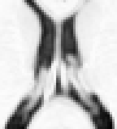
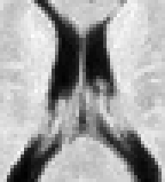
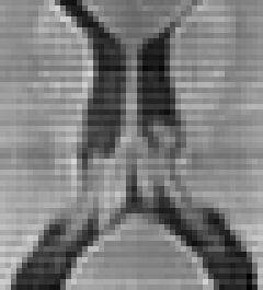
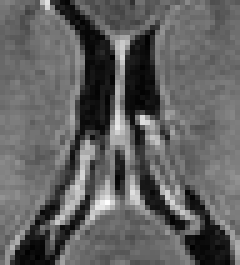
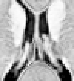
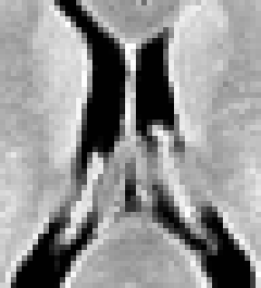
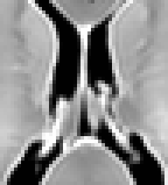
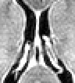
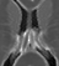
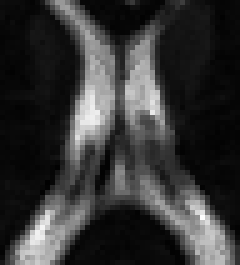
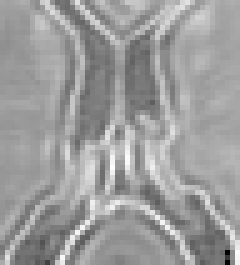
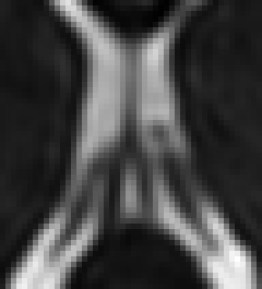
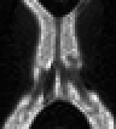
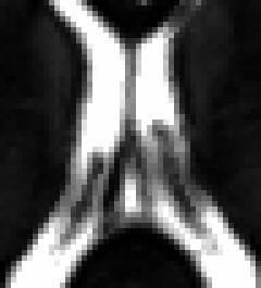
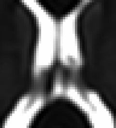
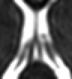
We split the data into two sets of nine for training and nine for testing. Bar charts in Figs. 1 and 2 show the mean and the bootstrapped 95% confidence interval of the T1-to-FLAIR and T1-to-T2 synthesis, respectively, for the quality metrics averaged over all testing data sets, for every normalization scheme and synthesis algorithm. We use the Wilcoxon signed-rank test to compare the distributions of each normalized method, for all metrics, against the corresponding unnormalized results per synthesis algorithm. We use a statistical significance level of $\alpha=0.05$ and show that this threshold is met in Figs. 1 and 2 with an asterisk above the corresponding bar. Figures 3 and 4 show results for the various synthesis algorithms with unnormalized training data (denoted raw) and normalized training data use the FCM approach.

The experiments show that synthesis results are robust to the choice of normalization algorithm, which are stable around the same levels across all metrics. This qualitative result, observed in Figs. 1 and 2, is reinforced with statistical tests. We use the Wilcoxon signed-rank test (with Bonferroni correction) to show statistically significant difference between any of the presented normalization algorithms for each metric ($\alpha=0.05$); however, no normalization algorithm consistently met this threshold for any metric with any synthesis algorithm in either T1-to-FLAIR or T1-to-T2 synthesis. An interesting finding is that—in T1-to-T2 synthesis—the random forest regressor qualitatively performs more robustly on unnormalized data, but both the DNN and polynomial regression methods fail; in terms of NCC, the DNN synthesis has zero mean because of negative correlation in some of the testing results.

Failure cases of synthesis in T1-to-FLAIR and T1-to-T2 unnormalized images are shown in Figs. 3 and 4, respectively, which can be compared to the successfully synthesized FCM-normalized images in the same figures. We discuss in the following section.

Figure 1: T1-to-FLAIR Quality Metrics: Raw corresponds to synthesis using unnormalized images, ZS to Z-score normalized images, and WS to WhiteStripe normalized images. Statistical significance (denoted by *) for each experiment is compared to Raw ($p<0.05$). The error bars represent the 95% confidence interval.

Figure 2: T1-to-T2 Quality Metrics: Raw corresponds to synthesis using unnormalized images, ZS to Z-score normalized images, and WS to WhiteStripe normalized images. Statistical significance (denoted by *) for each experiment is compared to Raw ($p<0.05$). The error bars represent the 95% confidence interval.

PR	RF	DNN	Truth

Figure 3: T1-to-FLAIR Synthesis results: Shown are the results of synthesis using unnormalized (top row) and FCM normalized images (bottom row). The unnormalized DNN result represents a failure of image synthesis.

PR	RF	DNN	Truth

Figure 4: T1-to-T2 Synthesis results: Shown are the results of synthesis using unnormalized (top row) and FCM normalized images (bottom row). The unnormalized DNN result represents a failure of image synthesis.

4 DISCUSSION AND CONCLUSION

We have shown that: 1) synthesis methods are substantially improved with the addition of an intensity normalization pre-processing step, especially DNN synthesis; 2) synthesis is robust to the choice of normalization method as we see no statistically significant difference in the presented normalization methods.

The failure cases shown in Figs. 3 and 4 results from the histogram of a particular input T1-w image being different than the majority of T1-w images the model was trained on. In this case, the problem histogram is compressed such that the grey matter peak was nearly aligned with the average location of the WM peaks for all but one of the training set (where the outlier on the training set also has the grey matter peak in the vicinity of the WM peak average for the training set).

The fact that we fail to synthesize unnormalized images correctly in the best case scenario—all of our training and testing images came from the same cohort acquired on the same scanner with the same pulse sequence and all of the images are of healthy patients—points to the importance of intensity normalization as a preprocessing step in any synthesis pipeline. While the highlighted failure case is remarkable, the synthesized versions of the remaining images also exhibit more subtle failure. Specifically, we see poor correspondence in intensities between slices. That is, if you scan through the images on the plane through which the image was synthesized (in this case axial), the result appears like a reasonable synthesis; however, when the image is viewed in the saggital plane we see significant variation in the intensities of neighboring slices and this variation is not observed in the synthesis results of normalized images (see Fig. 5 for an example). While this slice-to-slice variation is partly due to using a 2D synthesis method, 2D synthesis is commonly used in state-of-the-art synthesis methods[2, 10, 11]. Since the DNN performs better across all metrics when the images are normalized, normalization is suggested as a pre-processing step before training or testing any sort of patch-based DNN.

Figure 5: T1-to-FLAIR DNN Synthesis Shown from left to right are the results of DNN synthesis using FCM normalized images, unnormalized images, and the ground truth.