dgreenrgb0,0.7,0
First passage under stochastic resetting in an interval
Abstract
We consider a Brownian particle diffusing in a one dimensional interval with absorbing end points. We study the ramifications when such motion is interrupted and restarted from the same initial configuration. We provide a comprehensive study of the first passage properties of this trapping phenomena. We compute the mean first passage time and derive the criterion on which restart always expedites the underlying completion. We show how this set-up is a manifestation of a success-failure problem. We obtain the success and failure rates and relate them with the splitting probabilities, namely the probability that the particle will eventually be trapped on either of the boundaries without hitting the other one. Numerical studies are presented to support our analytic results.
I Introduction
The paradigm of diffusion with stochastic resetting has paved our way of understanding restarted processes Restart1 ; Restart2 . Consider a Brownian particle which is being reset to a preferred configuration with certain rate. This simple yet pivotal model markedly captures the quintessential features of such processes. There are two cornerstones of this phenomena. In the first case, one is interested in the concentration density of the particles performing such stochastic dynamics. In particular, it has been shown that resetting renders non-equilibrium steady states in generic stochastic processes Restart1 ; Restart2 ; KM ; Restart3 ; restart_conc1 ; restart_conc2 ; restart_conc3 ; restart_conc4 ; restart_conc5 ; restart_conc6 ; restart_conc7 ; restart_conc8 ; restart_conc9 ; restart_conc11 ; restart_conc12 ; restart_conc15 ; restart_conc16 ; restart_conc17 ; restart_conc18 ; restart_conc21 ; tethered ; localtimer ; Satya-refractory ; Satya-RT . Canonical examples are diffusion in free space Restart1 ; Restart2 or in a potential landscape restart_conc2 . These studies have also been extended to systems where resets are intermittent restart_conc3 or the waiting times between reset events are governed by a generic time distribution Restart4 ; Restart5 . Moreover, dynamics with resetting exhibit many interesting transient features such as relaxation of the density Restart4 ; restart_conc5 to the steady state and its transport properties transport1 ; transport2 .
Second, restart has emerged as a conceptual framework to study search processes Restart-Search1 ; Restart-Search2 ; Restart-Search3 ; Chechkin ; restart_conc19 ; restart_conc20 ; ReuveniPRL ; PalReuveniPRL ; Optimization ; drift-diffusion ; branching . Consider a simple diffusive searcher looking for a target. It is well known that the mean search time diverges thus making such strategies undesirable RednerBook ; MetzlerBook ; Schehr-review ; Benichou-review . On the contrary, stochastic resetting works in advantage by facilitating long moves from arbitrary location to the resetting location therefore cutting short those long trajectories which are detrimental. Thus restart works in favor of fast completion which otherwise would hinder. This simple observation has led the researchers to study first passage under generic restart mechanisms. Moreover, it has been demonstrated that it is even possible to find an optimal restart rate which can minimize the mean first passage time. Remarkably, one discovers various universality classes displayed by any restarted processes which are at optimality ReuveniPRL ; PalReuveniPRL ; Optimization .
The subject of resetting or restart has been in the limelight recently due to its numerous applications in many interdisciplinary fields. Apart from applications in search processes or animal foraging, restart has been found to be an indispensable part of chemical reactions Restart-Biophysics1 and randomized computer algorithms restart-CS1 . Further progress has seen applications of restart mechanisms in biophysics Restart-Biophysics2 ; Restart-Biophysics3 ; Restart-Biophysics4 , stochastic thermodynamics restart_thermo1 ; restart_thermo2 , and quantum mechanics Quantum1 ; Quantum2 .
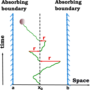
In this paper, we have investigated the motion of a Brownian particle (subjected to resetting) confined in a box in one dimension. The boundaries are absorbing (Fig. 1). In other words, they can be called targets or possible outcomes. In our set-up, we have two distinct possible outcomes: While the absorption at ‘’ can be defined as a failure or unwanted outcome, absorption at ‘’ can be coined as a success or anticipated outcome. If the underlying process completes prior to reset, then the process immediately ends. Otherwise, restart occurs: the particle is taken back to and allowed to start again given that it was not absorbed meanwhile. Thus, this model is reminiscent of a first passage process under restart which has different possible outcomes. Another example of such kind is a Bernoulli-like first passage process, which can also end with one of two possibilities. This set-up was studied recently in Ref. Optimization within the general framework of first passage under restart PalReuveniPRL . In Ref. Optimization , the authors have shown how restart can affect the success or failure probabilities of a Bernoulli trial. Moreover, it was shown that there are optimal restart rates which could maximize or minimize these outcome probabilities. We investigate akin properties by following the motion of the Brownian particle in the box, and illustrate that by tuning the restart rate it is possible to manipulate the process to complete in a desired way. Furthermore, we extend our study to demonstrate how restart can overall accelerate or hinder the completion of the process. We provide numerical studies to support our results. A similar study on diffusion with resetting in a bounded domain was studied recently in Ref. restart_conc8 . However, the boundaries were taken reflecting and an absorbing potential was introduced inside the interval. So, our set-up is very different from that of Ref. restart_conc8 .
The paper is organized in the following way. We first compute the survival probability which serves as an essential result of the paper. We illustrate two different methods, namely the backward Fokker-Planck approach (Sec. II.1) and the renewal formalism (Sec. II.2) to derive this result. This, in turn, allows us to compute the unconditional mean first passage time as a function of restart rate. This we do in Sec. III. We derive a closed form expression for the unconditional mean first passage time in Sec. III.1. Using that, we extract the essential criterion which has to be respected for restart to mitigate the completion in Sec. III.2. We study the optimal restart rate in Sec. III.3. Sec. IV is devoted to the conditional exit times. We compute the success, failure rates in Sec. IV.1 and their respective probabilities in Sec. IV.2. Furthermore, connections between the unconditional and conditional probabilities are analyzed in details in Sec. IV.2. Optimization properties of these probabilities are discussed in Sec. IV.3. Central results of this paper are summarized in Sec. V with a future outlook. The Appendix contains proofs of some our central results.
II Survival Probability
We consider a Brownian particle, initially located at , diffusing in an interval in one dimension. The particle can get absorbed by any of these boundaries. In addition, the particle is stochastically reset to the initial position with a constant rate . We are interested in the first passage properties of the particle to see the trade-off between the resetting and the natural absorption of the particle. To see this, we first provide a through analysis of the survival probability , defined as the probability that the particle has hit neither of the boundaries until time in the presence of resetting, starting from any . In other words, it estimates the probability that the particle survives (within the interval) until time . We present two different approaches to derive our results on the survival probability in the presence of resetting.
II.1 Backward Fokker Planck approach
It is quite well known that using the backward Fokker Planck equation can be an advantageous approach to treat the first passage properties. In this case, one first considers the initial position as a variable, and then solve the backward Fokker Planck equation with suitable boundary conditions self-consistently. To this end, we now consider the initial position to be (which is a variable), while keeping resetting position to be fixed. We solve the equations and at the end set to be . Following Ref. Restart1 , the backward Fokker Planck equation for the survival probability then reads
| (1) |
where the boundary conditions are and the initial condition is . The Laplace transform then satisfies Restart1
| (2) |
where . Solving Eq. (2) with the above boundary conditions, and finally setting , we obtain the following expression for the survival probability in the Laplace space
| (3) |
where we have defined
| (4) |
and . In the case of one absorbing boundary located at one recovers by setting . Substituting this expression in Eq. (3), we find , as derived earlier in Ref. Restart1 .
II.2 Renewal approach
One can also realize the restarted processes within the elegant formalism of renewals where one makes use of the fact that upon each reset, the system renews itself. Following Ref. Restart4 , we can write the survival probability in the following way
| (5) |
where is the survival probability of the particle in the interval upto time in the absence of resetting. Eq. (5) has a simple interpretation. The first term on the right hand side implies that the particle survives until time without experiencing any reset event. The second term considers the possibility when there are multiple reset events. One can then look at a long trajectory where the last reset event had occurred at time , and after that there has been no reset for the duration . This probability is given by . But then this has to be multiplied by , i.e., the probability that the particle survives until time with multiple reset events and , i.e., the survival probability of the particle for the last non-resetting interval Restart4 . The Laplace transform then satisfies
| (6) |
where is the Laplace transform of . Following Refs. RednerBook ; MetzlerBook ; Schehr-review , we use the well-known expression for
| (7) |
where are the eigenfunctions with . Also is the rate at which the -th eigenmode decays with time. Thus the longest decay time characterizes the diffusing dynamics within the interval. Making use of the renewal formula [Eq. (6)], we obtain an expression of the Laplace transform ,
| (8) |
where
| (9) |
The expressions obtained via backward Fokker-Planck equation (Eq. (3)) or the renewal approach (Eq. (8)) are equivalent (see Appendix A for more details).
II.3 Position density of the particle
In the presence of two absorbing boundaries, the particle will be absorbed in the absence of resetting. Question is by relocating the particle repeatedly to its initial position whether one can still find a finite probability to observe the particle within the domain at large time. To see this, we first define the position density , which estimates the probability of finding the particle at at time given that it had started from in the presence of multiple resetting at . We can write a time dependent equation for the position density using a renewal formalism
| (10) | |||||
where is the probability density of finding the particle in the interval in the absence of resetting. Also, recall that is the survival probability until time . We emphasize that Eq. (10) can be interpreted in an identical manner as in Eq. (5). By taking Laplace transform on both sides of Eq. (10) and using Eq. (6), we find
| (11) |
The probability density is a classical result and known from the literature RednerBook
| (12) |
Using the Laplace transform of and substituting in Eq. (11) one obtains
| (13) | |||||
In order to find the asymptotic behavior of the position density (i.e., the steady state), we can make use of the final value theorem. The theorem asserts that Restart4 . By doing a expansion on the right hand side of Eq. (13), we note that there are no terms which are of order , for any resetting rate . This indicates an absence of finite value for the probability density in the large time limit i.e., no particle will survive given long enough time. Once the spread of the concentration becomes comparable to the interval size, the flux of probability through the boundaries becomes significant and the density inside the interval decays rapidly despite the resetting dynamics.
III Unconditional First Passage Time
In the preceding section, we have studied the survival probability of the Brownian particle in the interval bounded between and . It is only natural to ask the time it will take for the particle to exit or get absorbed for the first time by any of these boundaries in the presence of resetting at . These first passage times are random, and one is in general interested in the statistics of such time. In this section, we will focus on this time statistics in the presence of resetting. It is worth mentioning that this situation is analogous to a first passage process with multiple outcomes, and the cumulative first passage time statistics for any possible outcome is statistically identical to that of unconditional first passage time.
III.1 Mean first passage time
We will first characterize the average time it takes for a particle to exit through any of the boundaries. We call this unconditional mean first passage time, denoted by . By noting that , where , is the unconditional first passage time density. Hence, by doing integration by parts, one can write
| (14) |
where we have used Eq. (3). Further simplification using Eq. (4) leads us to the following expression for the mean first passage time
| (15) |
where
| (16) |
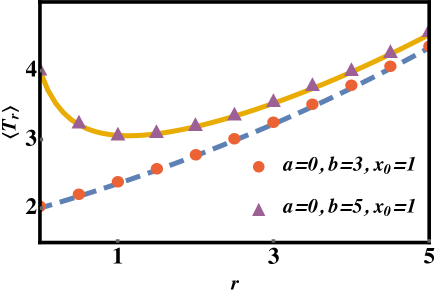
In the limit of vanishing restart rate (), we obtain RednerBook . We can also obtain using the renewal formula obtained in Ref. PalReuveniPRL , which requires a prior knowledge of the underlying first passage time distribution (without resetting). In Fig. 2, we have plotted using Eq. (15) as a function reset rate for two different set of parameters: (i) , and (ii) for fixed . In the first case increases monotonically with rate , unlike in the latter case. In fact, in the second case, restart lowers the mean first passage time and thus accelerating the completion. Nevertheless, it is not evident what sets the criterion for restart either to prolong or expedite the completion. To characterize this transition, we do a detailed analysis of the restart criterion in the next subsection.
III.2 Analysis of the restart criterion
It is well understood from the theory of first passage under restart that restart has the ability to expedite the underlying completion if , where CV stands for the ratio between the standard deviation and the mean first passage time of the underlying (i.e., without restart) first passage time process. One can arrive at this criterion by simply setting PalReuveniPRL . In the case of a diffusive first passage process (where the first passage time distribution is given by Lévy-Smirnov distribution RednerBook ; MetzlerBook ; Schehr-review ), the criterion is inherently satisfied. Thus restart will always expedite the completion of such process. On the other hand, as we have shown in Fig. 2, restart can both expedite or hinder the completion of a diffusive motion in an interval. To understand the criterion in terms of the relevant parameters of the system, we first set the criterion which yields
| (17) |
where and . We arrive at this expression by recalling that the mean first passage time is given by and the second moment is given by . Obtaining from Eq. (3) by taking limit yields . Substituting these expressions in the criterion , we obtain Eq. (17). A crucial observation is that the criterion is independent of the diffusion coefficient (hence, the motion of the particle), thus only the combination of length scales will set the criterion. Further simplifications can be made if we choose . Then from Eq. (17), we obtain . This determines the domain in which restart expedites the completion of the underlying process: , where . Hence, if the particle starts closer to either of the boundaries (i.e. , or ), the completion will be accelerated. On the other hand, if , restart will not be beneficial. This means if the particle starts in the region which is centered around , restart will only prolong the completion.
III.3 Optimal restart rate
The above analysis asserts that restart can accelerate the completion of the underlying process in certain regimes of the parameter values. This regime was fully characterized in the previous section and also will be a focus of our analysis here. In this regime, restart not only expedites the completion, one also observes that the mean first passage time can be minimized at a certain value of restart rate. To further illustrate on this optimal restart rate, we first note that Eq. (15) can be scaled in the following way
| (18) |
after setting the left boundary . In Eq. (18), we have defined a new scaling variable and the scaling function , which is now a function of restart rate for a given set of , is given by
| (19) |
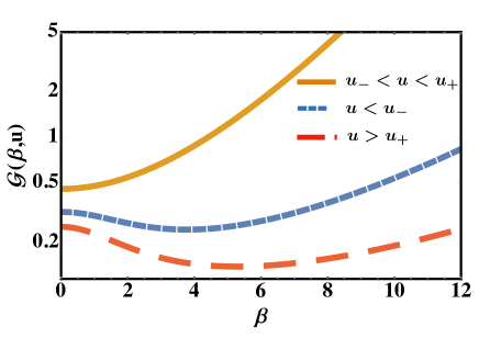
To find the optimal restart rate, one sets . This, in turn, gives the optimal restart rate , in terms of . In Fig. 3, we optimize the scaling function numerically as a function of in three different regimes of defined by the domain . It is evident from Fig. 3 that when , the function is minimum at , meaning can not be made lower by introducing a finite restart rate. On the other hand, when , we see that the scaling function is minimized at a finite implying that the mean first passage time is optimized at a finite restart rate.
IV Conditional First Passage Time
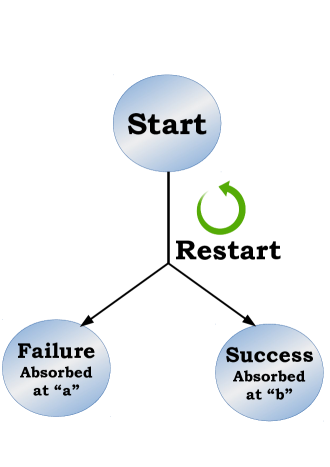
So far, we have focused only on the unconditional mean first passage time i.e., the exit time irrespective of boundaries or the particular choice of outcomes within the success-failure set-up (see Fig. 4). We devote this section to study observables conditioned on the ‘outcome of our choice’. Examples of such observables are: conditional mean exit times from boundary ‘’ or ‘’. Recalling that a ‘successful’ event was defined by an absorption at the boundary ‘b’ and ‘failure’ by absorption at the boundary ‘a’, the conditional exit times provide us estimations of success or failure rates. Another natural quantity to investigate would be the splitting probability namely the probability to escape through a specified boundary without hitting the other ones which is, in fact, a measure of success or failure probability. Interestingly, restart could optimize the success or failure probabilities. In other words, by modulating restart rate one can reduce the occurrence of failure events, while facilitating the probability of success to its maximum.
IV.1 Mean conditional exit times
Mean conditional exit time is the average time for the particle to hit a specific boundary without hitting the other one. Let us define to be the conditional mean exit times through the boundaries and respectively. To compute this time statistics, it is best to first measure the flux of current flowing through each one of these boundaries. Probability flux current at any point in space at time is defined by . The exit times and the flux are then related to each other by the following relation RednerBook
| (20) |
where denote the currents at each of the boundaries, as given below:
| (21) |
The expression for the conditional exit times Eq. (20) can be understood as follows. Note that the currents, defined in Eq. (21), are identical to the conditional first passage time densities through each one of these boundaries. Hence, to obtain , one needs to average over these conditional first passage time densities. The conditional mean exit times in Eq. (20) can be rewritten in terms of the currents in Laplace space
| (22) |
where , satisfy
| (23) |
Substituting in Eq. (23) from Eq. (13), we get the following expressions for the currents
| (24) |
where
| (25) | |||||
Now using Eq. (24) and Eq. (25) in Eq. (22) one gets the exact formula for the conditional exit times
| (26) |
where
The success and failure rates are then given by
| (28) |
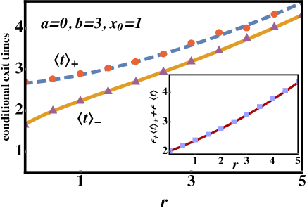
Note that the conditional exit times are monotonic function of the restart rate, and moreover they diverge as restart rate increases (see Fig. 5). In the limit of vanishing restart rate, the mean conditional exit times through the boundaries and are given by
| (29) |
In Fig. 5, we have plotted simulation data against the theoretical formulas (obtained in Eq. (26)) for conditional exit times as a function of restart rate, for a system with boundaries and the resetting position , when . The limit values are also in accordance with Eq. (29), as expected.
IV.2 Splitting probabilities
We present now analytical expressions for the splitting probabilities, the probability that the process starting at and evolving in a box hits the right boundary before hitting the left boundary at , and vice-versa. Let us define these probabilities as respectively. Thus, denote the success and failure probability respectively. To compute these probabilities, one needs to integrate the current flux flowing through each of the boundaries over the time as shown below
| (30) |
Using the formulae for from Eq. (24) and substituting for , we obtain the following expressions for the splitting probabilities:
| (31) | |||||
| (32) |
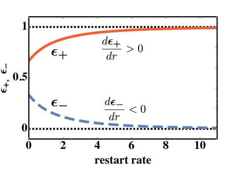
At limit, these probabilities of winning or losing will be given by . Further taking , we find . Thus the probability of reaching one end point is just the relative distance to the other end point, which is quite remarkable RednerBook . On the other hand, in the large limit, behavior of splitting probabilities has a strong dependence on the resetting (initial) position . If , we have i.e., the particle which starts (and resets) on the positive side of the middle of the interval eventually reaches the boundary with probability one. Conversely, when , one finds , which is exactly one would expect. However, if then we have for any restart rate. In Fig. 6, we have plotted the splitting probabilities as a function of restart rate. It is also evident from the figure that these probabilities saturate either to maximum or minimum as a function of restart rate. In Sec. IV.3, we will show how one can utilize this particular property to engineer restart as a tool to the fulfillment of the required outcomes.
A careful observation of the exact expressions for the conditional exit times and the splitting probabilities immediately leads us to establish the following relation
| (33) |
which holds for any restart rate. This means that the unconditional mean exit time (independent of which side is exited) is the appropriately weighted average of the conditional mean exit times to each boundary. These weights are the conditional splitting probabilities. But this is no surprise and can be understood by simple path enumeration. The splitting probability sums over all the paths that start from and exit through boundary without hitting the boundary . Thus, , where denotes the weight of a single trajectory from to that avoids . On the other hand, is the exit time through boundary conditioned on the fact that it has survived the boundary . Thus, , where is the exit time of a specific trajectory that starts at through a boundary. One can use a similar argument for and . Eq. (33) is also demonstrated in the inset of Fig. 5.
It is also interesting to examine the behavior of the exit times as a function of resetting (initial) position . Note that, when (i.e., the particle starts from the middle of the interval) we get , and by using Eq. (33). Moreover, if the particle starts from either or , the particle will get absorbed immediately, so that . However, note that , which is quite non-intuitive. This is because is conditioned on the fact that the particle survives boundary even if it had started from . There will be rare trajectories which will do so, and these will contribute to . A similar argument justifies the complementary case . Since these limits are symmetric with respect to the interval, they are identical and given by . In Fig. 7, we have plotted the unconditional and the conditional exit times as a function of different . In particular, we have assumed and , where we have varied . As expected, in the symmetric case, i.e., when , the system does not distinguish between left and right boundaries so that . The other limits are also evident from the figure.
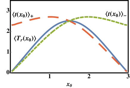
A closer look at Fig. 7 reveals that both the conditional exit times are non-monotonic functions of the initial position . To understand this behavior of with respect to , we consider the slope
| (34) |
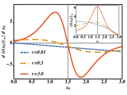
We investigate as a function of by varying as a parameter. In the limit, which is zero only at , otherwise negative. Thus is strictly monotonic as a function of . In sharp contrast, as , we note that only when . In fact, both and will have a single maximum at . While for any finite , the slope becomes zero for . Consequently, the maximum of the conditional exit time spans in the range . It is worth emphasizing that such non-monotonic behavior of is robust to restart, and is lost in the absence of restart when always become monotonic functions. We have plotted as a function of for different values of restart rate in Fig. 8. In the inset we have given plots for as a function of for the values of used in the main plot. A similar analysis also follows for which we skip here to avoid redundancy.
IV.3 Restart optimizes success and failure probabilities
In the previous sections, we showed how restart can optimize the mean completion time of a first passage process under restart. In addition, restart can also optimize the success or failure probabilities. This will be the focus of this section. As mentioned before, similar questions were posed and surveyed in a generic set-up in Ref. Optimization . We will refer to Ref. Optimization for the general proofs which was based on the general approach proposed by one of the current authors PalReuveniPRL . However, in this paper we have taken different approach and presented alternative proofs of some of the central results.
Let be the conditional (success and failure) exit times and the unconditional exit time (also considered in Sec. III.1) in the absence of restart. The density of the latter is given by , where is given by Eq. (7). Using this, one can write the Laplace transform as
| (35) |
The conditional exit time distributions in the absence of restart are identical to the conditional current fluxes through each one of these boundaries [see e.g., Eq. (21) at the limit]. Hence, one can write
| (36) |
One can now compute the Laplace transforms evaluated at using Eq. (36). Furthermore, they can be utilized to recover the success and failure probabilities . These two quantities are related by
| (37) |
and moreover, one can show
| (38) |
See Appendix B and Appendix C for a detailed derivation of these two results. It is important to note that the proofs presented here offer an alternative derivation in comparison to that of demonstrated in Ref. Optimization . Remarkably, Eq. (38) offers us a deep insight on how restart could maximize or minimize the chances of our desired outcomes. To see this, let us first consider the case when (see Fig. 6 for instance). Eq. (38) then tells us that so that the mean conditional time to exit through the boundary (equivalently rendering ‘success’) is reduced by regulating the restart rate . In other words, by carefully choosing a restart rate, the process can be completed faster in our desired way. On the other hand, when , we observe . This implies that the exit time through the boundary will take longer time, and thus by regulating restart, one can hinder the outcome of ‘failure’. The present model at our disposal provides a nice demonstration of how using the restart mechanism one could moderate the chances of desired outcomes of a first passage process that can, in principle, end with multiple eventualities.
V Conclusion
First passage with restart under various set-up has been a focal point in recent studies. The fact that restart has the ability to speedup underlying completion is noteworthy, and this is perhaps the fingerprint of most of these studies. In this paper, we have studied first passage properties of a Brownian particle in a bounded domain in the presence of stochastic resetting. We have shown how this set-up can be visualized as a success-failure problem. We have computed the unconditional mean first passage time and characterized a rich optimization phenomena with respect to the restart rate. We extend the methodology to give estimation of success and failure rates, and furthermore show how restart could optimize the success and failure probabilities. Finally we would like to emphasize that in this problem, we have considered sharp binary outcomes in the sense that the outcomes are either success (full absorption at ‘’) or failure (full absorption at ‘’). However, these outcomes may not necessarily be sharp, but rather mixed. In other words, the Brownian particle can mix the probabilities of getting absorbed or reflected with certain rate at each boundary reactive . We believe that the formalism presented in this paper should be useful to tackle such problems, and is left for future studies.
VI Acknowledgments
We thank Anupam Kundu for many illuminating discussions. Arnab Pal acknowledges support from the Raymond and Beverly Sackler Post-Doctoral Scholarship.
Appendix A Equivalence between Eq. (3) and Eq. (8)
In this section, we will show the equivalence between Eq. (3) and Eq. (8). To see this, let us first recall from Eq. (8) that contains the following summation both in the numerator and the denominator. To evaluate this sum, we explicitly use the expressions for and , and rewrite in the following way
| (39) |
where we have defined , such that . We can now make use of the following identities to compute the sums
| (40) | |||||
and
Using the identities above, we can now convert the sums in Eq. (39). After doing a bit of simplification we arrive at
where is given by Eq. (4)
| (42) |
Substituting in Eq. (8), we obtain
which is indeed Eq. (3), as reported earlier.
Appendix B Proof of Eq. (37)
In this section, we provide a proof for the following relations
| (43) |
Here, we will demonstrate the proof for while an analysis for can also be made in a similar manner. Let us first recall the definition from Eq. (30)
| (44) |
where follows from Eq. (23)
| (45) |
which can be rewritten as
by replacing with using Eq. (11). Setting in the above equation, we find
| (47) | |||||
We now note that
| (48) | |||||
where is the survival probability (see the results from Sec. IV.3). Doing an integration by parts in Eq. (48), we find
| (49) |
On the other hand, let us define
| (50) | |||||
where was introduced in Eq. (36). But also note that . Hence
| (51) | |||||
Thus, we have proven
| (52) |
Using Eq. (49) and Eq. (52) in Eq. (47), we finally arrive at the following relation we were seeking after
| (53) |
Appendix C Proof of Eq. (38)
In this Appendix, we will provide the proofs of the following relations
| (54) |
Like in the preceding Appendix, here we will only demonstrate the proof for and leave for a likewise proof. We start by writing a renewal equation for the current given by
Such kind of renewal equations served as a bedrock already for many of our central results. Taking Laplace transform on both sides of the above equation, we obtain
| (56) | |||||
where we have used Eq. (6). Now, recall from Eq. (22)
| (57) |
which can be rewritten as
| (58) |
Substituting from Eq. (56) in the above equation gives us
| (59) |
We have already proven in the last section that [see e.g., Eq. (51)], such that . Furthermore, it is also evident from Eq. (51) that
| (60) |
On the other hand, note that
| (61) | |||||
Now from Eq. (49), recall that . Taking derivative on both sides with respect to , we find
| (62) |
Substituting from the above expression in Eq. (61), we arrive at
Replacing all the expressions obtained from Eq. (60) and Eq. (LABEL:fracs1) in Eq. (59), we finally arrive at
| (64) | |||||
which is our desired result Eq. (38). This completes the proof.
References
- (1) Evans, M.R. and Majumdar, S.N., 2011. Diffusion with stochastic resetting. Physical review letters, 106(16), p.160601.
- (2) Evans, M.R. and Majumdar, S.N., 2011. Diffusion with optimal resetting. Journal of Physics A: Mathematical and Theoretical, 44(43), p.435001.
- (3) Evans, M.R., Majumdar, S.N. and Mallick, K., 2013. Optimal diffusive search: nonequilibrium resetting versus equilibrium dynamics. Journal of Physics A: Mathematical and Theoretical, 46(18), p.185001.
- (4) Montero, M. and Villarroel, J., 2013. Monotonic continuous-time random walks with drift and stochastic reset events. Physical Review E, 87(1), p.012116.
- (5) Gupta, S., Majumdar, S.N. and Schehr, G., 2014. Fluctuating interfaces subject to stochastic resetting. Physical review letters, 112(22), p.220601.
- (6) Pal, A., 2015. Diffusion in a potential landscape with stochastic resetting. Physical Review E, 91(1), p.012113.
- (7) Eule, S. and Metzger, J.J., 2016. Non-equilibrium steady states of stochastic processes with intermittent resetting. New Journal of Physics, 18(3), p.033006.
- (8) Durang, X., Henkel, M. and Park, H., 2014. The statistical mechanics of the coagulation–diffusion process with a stochastic reset. Journal of Physics A: Mathematical and Theoretical, 47(4), p.045002.
- (9) Majumdar, S.N., Sabhapandit, S. and Schehr, G., 2015. Dynamical transition in the temporal relaxation of stochastic processes under resetting. Physical Review E, 91(5), p.052131.
- (10) Evans, M.R. and Majumdar, S.N., 2014. Diffusion with resetting in arbitrary spatial dimension. Journal of Physics A: Mathematical and Theoretical, 47(28), p.285001.
- (11) Méndez, V. and Campos, D., 2016. Characterization of stationary states in random walks with stochastic resetting. Physical Review E, 93(2), p.022106.
- (12) Christou, C. and Schadschneider, A., 2015. Diffusion with resetting in bounded domains. Journal of Physics A: Mathematical and Theoretical, 48(28), p.285003.
- (13) Chatterjee, A., Christou, C. and Schadschneider, A., 2018. Diffusion with resetting inside a circle. Physical Review E, 97(6), p.062106.
- (14) Falcón-Cortés, A., Boyer, D., Giuggioli, L. and Majumdar, S.N., 2017. Localization transition induced by learning in random searches. Physical review letters, 119(14), p.140603.
- (15) Falcao, R. and Evans, M.R., 2017. Interacting Brownian motion with resetting. Journal of Statistical Mechanics: Theory and Experiment, 2017(2), p.023204.
- (16) Montero, M., Masó-Puigdellosas, A. and Villarroel, J., 2017. Continuous-time random walks with reset events: Historical background and new perspectives. J. Eur. Phys. J. B 90: 176.
- (17) Majumdar, S.N., Sabhapandit, S. and Schehr, G., 2015. Random walk with random resetting to the maximum position. Physical Review E, 92(5), p.052126.
- (18) Meylahn, J.M., Sabhapandit, S. and Touchette, H., 2015. Large deviations for Markov processes with resetting. Physical Review E, 92(6), p.062148.
- (19) Boyer, D., Evans, M.R. and Majumdar, S.N., 2017. Long time scaling behaviour for diffusion with resetting and memory. Journal of Statistical Mechanics: Theory and Experiment, 2017(2), p.023208.
- (20) Shkilev, V.P., 2017. Continuous-time random walk under time-dependent resetting. Physical Review E, 96(1), p.012126.
- (21) Giuggioli, L., Gupta, S. and Chase, M., 2018. Comparison of two models of tethered motion, J. Phys. A 52, 075001 (2019).
- (22) Pal, A., Chatterjee, R., Reuveni, S. and Kundu, A., 2019. Local time of diffusion with stochastic resetting, arXiv preprint arXiv:1902.00907.
- (23) Evans, M.R. and Majumdar, S.N., Effects of refractory period on stochastic resetting, J. Phys. A 52, 01LT01 (2018).
- (24) Evans, M.R. and Majumdar, S.N., 2018. Run and tumble particle under resetting: a renewal approach. Journal of Physics A: Mathematical and Theoretical, 51(47), p.475003.
- (25) Pal, A., Kundu, A. and Evans, M.R., 2016. Diffusion under time-dependent resetting. Journal of Physics A: Mathematical and Theoretical, 49(22), p.225001.
- (26) Nagar, A. and Gupta, S., 2016. Diffusion with stochastic resetting at power-law times. Physical Review E, 93(6), p.060102.
- (27) Masó-Puigdellosas, A., Campos, D. and Méndez, V., 2018. Stochastic processes subject to a reset-and-residence mechanism: transport properties and first arrival statistics, J. Stat. Mech. (2019) 033201.
- (28) Masó-Puigdellosas, A., Campos, D. and Méndez, V., 2018. Transport properties and first arrival statistics of random searches with stochastic reset times, Phys. Rev. E 99, 012141 (2019).
- (29) Kusmierz, L., Majumdar, S.N., Sabhapandit, S. and Schehr, G., 2014. First order transition for the optimal search time of Lévy flights with resetting. Physical review letters, 113(22), p.220602.
- (30) Kusmierz, L. and Gudowska-Nowak, E., 2015. Optimal first-arrival times in Lévy flights with resetting. Physical Review E, 92(5), p.052127.
- (31) Bhat, U., De Bacco, C. and Redner, S., 2016. Stochastic search with Poisson and deterministic resetting. Journal of Statistical Mechanics: Theory and Experiment, 2016(8), p.083401.
- (32) Chechkin, A. and Sokolov, I.M., 2018. Random search with resetting: a unified renewal approach. Physical review letters, 121(5), p.050601.
- (33) Husain, K. and Krishna, S., 2016. Efficiency of a Stochastic Search with Punctual and Costly Restarts. arXiv preprint arXiv:1609.03754.
- (34) Campos, D. and Méndez, V., 2015. Phase transitions in optimal search times: How random walkers should combine resetting and flight scales. Physical Review E, 92(6), p.062115.
- (35) Reuveni, S., 2016. Optimal stochastic restart renders fluctuations in first passage times universal. Physical review letters, 116(17), p.170601.
- (36) Pal, A. and Reuveni, S., 2017. First Passage under Restart. Physical review letters, 118(3), p.030603.
- (37) Belan, S., 2018. Restart could optimize the probability of success in a Bernoulli trial. Physical review letters, 120(8), p.080601.
- (38) Ray, S., Mondal, D. and Reuveni, S., 2018. Péclet number governs transition to acceleratory restart in drift-diffusion. arXiv preprint arXiv:1811.08239.
- (39) Pal, A., Eliazar, I. and Reuveni, S., 2019. First passage under restart with branching. Physical review letters, 122(2), p.020602.
- (40) Redner, S., 2007. A Guide to First-Passage Processes. A Guide to First-Passage Processes, by Sidney Redner, Cambridge, UK: Cambridge University Press, 2007.
- (41) Metzler, R., Redner, S. and Oshanin, G., 2014. First-Passage Phenomena and Their Applications (Vol. 35). Singapore: World Scientific.
- (42) Bray, A.J., Majumdar, S.N. and Schehr, G., 2013. Persistence and first-passage properties in nonequilibrium systems. Advances in Physics, 62(3), pp.225-361.
- (43) Bénichou, O., Loverdo, C., Moreau, M. and Voituriez, R., 2011. Intermittent search strategies. Reviews of Modern Physics, 83(1), p.81.
- (44) Reuveni, S., Urbakh, M. and Klafter, J., 2014. Role of substrate unbinding in Michaelis-Menten enzymatic reactions. Proceedings of the National Academy of Sciences, 111(12), pp.4391-4396.
- (45) Luby, M., Sinclair, A. and Zuckerman, D., 1993, June. Optimal speedup of Las Vegas algorithms. In Theory and Computing Systems, 1993., Proceedings of the 2nd Israel Symposium on the (pp. 128-133). IEEE.
- (46) Rotbart, T., Reuveni, S. and Urbakh, M., 2015. Michaelis-Menten reaction scheme as a unified approach towards the optimal restart problem. Physical Review E, 92(6), p.060101.
- (47) Robin, T., Reuveni, S. and Urbakh, M., 2018. Single-molecule theory of enzymatic inhibition. Nature communications, 9(1), p.779.
- (48) Roldán, É., Lisica, A., Sánchez-Taltavull, D. and Grill, S.W., 2016. Stochastic resetting in backtrack recovery by RNA polymerases. Physical Review E, 93(6), p.062411.
- (49) Fuchs, J., Goldt, S. and Seifert, U., 2016. Stochastic thermodynamics of resetting. EPL (Europhysics Letters), 113(6), p.60009.
- (50) Pal, A. and Rahav, S., 2017. Integral fluctuation theorems for stochastic resetting systems. Physical Review E, 96(6), p.062135.
- (51) Rose, D.C., Touchette, H., Lesanovsky, I. and Garrahan, J.P., 2018. Spectral properties of simple classical and quantum reset processes. Physical Review E 98, 022129.
- (52) Mukherjee, B., Sengupta, K. and Majumdar, S.N., 2018. Quantum dynamics with stochastic reset. Physical Review B 98, 104309.
- (53) Pal, A., Castillo, I.P. and Kundu, A., 2018. Motion of a Brownian molecule in the presence of reactive boundaries. arXiv preprint arXiv:1805.04762.