Online basis construction for goal-oriented adaptivity in the Generalized Multiscale Finite Element Method

Abstract

In this research, we develop an online enrichment framework for goal-oriented adaptivity within the generalized multiscale finite element method for flow problems in heterogeneous media. The method for approximating the quantity of interest involves construction of residual-based primal and dual basis functions used to enrich the multiscale space at each stage of the adaptive algorithm. Three different online enrichment strategies based on the primal-dual online basis construction are proposed: standard, primal-dual combined and primal-dual product based. Numerical experiments are performed to illustrate the efficiency of the proposed methods for high-contrast heterogeneous problems.

Keywords  Goal-oriented adaptivity, multiscale finite element method, online basis construction, flow in heterogeneous media.

1 Introduction

In this work, we propose an efficient goal-oriented framework for approximating quantities of interest for flow problems posed in heterogeneous media. Many problems arising from engineering involve heterogeneous materials which have strong contrasts in their physical properties. In general, one may model these so-called multiscale problems using partial differential equations (PDEs) with high-contrast valued multiscale coefficients. An important example is Darcy’s law describing flow in porous media, modeled here by the boundary value problem in the computational domain $\Omega\subset\mathbb{R}^{d}$ ($d=2,3$)

$$-\text{div}(\kappa(x)\nabla u)=f(x)\quad\text{in }\Omega,\quad u=0\quad\text{on }\partial\Omega.$$ (1)

The direct simulation of multiscale PDEs with accurate resolution can be costly as a relatively fine mesh is required to resolve the coefficients, leading to a prohibitively large number of degrees of freedom (DOF), a high percentage of which may be extraneous. Recently, these computational challenges have been addressed by the development of efficient model reduction techniques such as numerical homogenization methods [17, 18, 27, 31, 32] and multiscale methods [5, 6, 7, 22, 33, 34]. These methods have been shown to reduce the computational cost of the simulation, for instance approximating $u$ of (1). Here, we apply goal-oriented methods to further reduce the computational cost in the approximation of a quantity of interest.

We consider (1) with $f\in L^{2}(\Omega)$ given and for which $\kappa(x)$ satisfies $\kappa_{0}\leq\kappa(x)\leq\kappa_{1}$ for a.e. $x$ in $\Omega$ with constants $0<\kappa_{0}\ll\kappa_{1}.$ We proceed by posing (1) in its variational form

$$a(u,v)=f(v)\quad\forall v\in H_{0}^{1}(\Omega),$$ (2)

where $a(u,v):=\int_{\Omega}\kappa(x)\nabla u\cdot\nabla v\,\mathrm{d}{x}$ and $f(v):=\int_{\Omega}fv\,\mathrm{d}{x}$. We are interested in the case where $\kappa(x)$ is a heterogeneous coefficient with high-contrast, and model reduction is necessary to efficiently approximate the solution.

Next, we briefly describe the continuous Galerkin (CG) formulation of the generalized multiscale finite element method (GMsFEM) [7, 14], a systematic approach to multiscale model reduction. We start with the notion of fine and coarse grids. Let $\mathcal{T}^{H}$ be a conforming partition of the computational domain $\Omega$ with mesh size $H>0$. We refer to this partition as the coarse grid. Subordinate to the coarse grid, we define the fine grid partition (with mesh size $h\ll H$), denoted by $\mathcal{T}^{h}$, by refining each coarse element into a connected union of fine grid blocks. We assume the above refinement is performed such that $\mathcal{T}^{h}$ is a conforming partition of $\Omega$. Let $N_{c}$ be the number of interior coarse grid nodes and let $\{x_{i}\}_{i=1}^{N_{c}}$ be the set of coarse grid nodes of the coarse mesh $\mathcal{T}^{H}$. Let $N$ be the number of elements in the coarse mesh. Define the coarse neighborhood of the node $x_{i}$ by

$$\omega_{i}:=\bigcup\{K_{j}\in\mathcal{T}^{H}:x_{i}\in\overline{K}_{j}\},$$

that is, the union of all coarse elements which have the node $x_{i}$ as a vertex.

Let the fine-scale finite element space $V$ be the conforming piecewise linear finite element space corresponding to the fine grid $\mathcal{T}^{h}$ and let $u\in V$ be the fine-scale solution satisfying the variational problem

$$a(u,v)=f(v)\quad\forall v\in V.$$ (3)

Define the energy norm on $V$ by $\left\|u\right\|_{V}^{2}:=a(u,u)$.

For each coarse node $x_{i}$, we construct a so-called offline set of basis functions supported on the neighborhood $\omega_{i}$. These pre-computed multiscale basis functions are obtained from a local snapshot space and a local spectral decomposition defined on that snapshot space. The snapshot space contains a collection of basis functions that can capture most of the fine features of the solution. The multiscale basis functions are computed by selecting the dominant modes of the snapshot space through the local spectral problem. Once the basis functions are identified, the CG global coupling is given through the variational formulation

$$a(u_{ms},v)=f(v)\quad\forall v\in V_{\text{off}},$$

where $V_{\text{off}}$, called the offline space, is the space spanned by the multiscale basis functions. In order to obtain an efficient representation of solution, it is desirable to determine the number of basis functions per coarse neighborhood adaptively based on the heterogeneities of the coefficient $\kappa$. In [9], a residual based a posteriori error indicator is derived and an adaptive basis enrichment algorithm is developed under the CG formulation. In particular, it is shown that

$$\left\|u-u_{ms}\right\|_{V}^{2}\leq C\sum_{i=1}^{N_{c}}\left\|R_{i}\right\|^{2}_{V_{i}^{\ast}}\left(\lambda_{l_{i}+1}^{(i)}\right)^{-1},$$

where $V_{i}^{\ast}$ is the dual space to $V_{i}:=H^{1}_{0}(\omega_{i})\cap V$, $R_{i}\in V_{i}^{\ast}$ is the residual operator with respect to the multiscale solution $u_{ms}$ on $\omega_{i}$ and $\lambda_{l_{i}+1}^{(i)}$ is the smallest eigenvalue whose eigenvector is excluded in the construction of the offline space on coarse neighborhood $\omega_{i}$. Thus, local residuals of the multiscale solution together with the corresponding eigenvalues give indicators to the error of the solution in the energy norm. One can then enrich the multiscale space by selectively adding basis functions corresponding to the coarse neighborhoods in which indicators are large.

On the other hand, for some applications it can be beneficial to adaptively construct new online basis functions during the course of the adaptive algorithm to capture distant effects. In [8], such online adaptivity is proposed and mathematically analyzed. More precisely, when the local residual related to some coarse neighborhood $\omega_{i}$ is large, one may construct a new basis function $\phi_{i}\in V_{i}$ in the online stage by solving

$$a(\phi_{i},v)=R_{i}(v)\quad\forall v\in V_{i},$$

then adding $\phi_{i}$ as one of the basis functions of multiscale space. It is further shown that if the offline space $V_{\text{off}}$ contains sufficient information in the form of offline basis functions, then the online basis construction leads to an efficient approximation of the fine-scale solution.

The adaptivity procedures discussed above are designed with the aim of reducing the error in the energy norm. In some applications, one may be more interested in reducing error measured by some quantity of interest or function of the solution other than a norm. For example, in flow applications, one needs to obtain a good approximation of the pressure in locations where the wells are situated. Goal-oriented adaptivity [1, 4, 19, 21, 25, 26, 28, 30, 35] (and the references therein) can be used to more efficiently reduce the error in the quantity of interest without necessarily achieving the same rate of error reduction in a global sense. Goal-oriented adaptivity has been introduced within the setting of multiscale methodologies in for instance [2, 3, 29], where the authors review the framework of approximating a quantity of interest and investigate the use of this framework in a number of multiscale scientific applications (e.g. quasicontinuum models and molecular dynamics). In [23] the authors perform goal-oriented mesh refinement in the setting of numerical homogenization for nonlinear lattice elasticity problems. In [24], the a posteriori error estimate within the framework of multiscale finite element method was proposed; and, goal-oriented enrichment within the flexible GMsFEM framework with offline basis functions is discussed in [10, 11].

In this research, we develop an online basis construction for goal-oriented adaptivity within GMsFEM for (1). For a given linear functional $g:V\rightarrow\mathbb{R}$, referred to as the goal functional, we seek to approximate $g(u)$ where $u$ is the solution to (3). One may adaptively enrich the approximation space in order to reduce the goal-error defined by $\lvert g(u-u_{ms})\rvert$, where $u_{ms}$ is the latest multiscale solution. For the construction of goal-oriented adaptivity, the dual problem is considered based on $a^{\ast}(\,\cdot\,,\,\cdot\,)$, the formal adjoint of $a(\,\cdot\,,\,\cdot\,)$ which satisfies $a^{*}(w,v)=a(v,w)$. In the current symmetric linear case, the dual form is identical to the primal. For the primal problem $a(u,v)=f(v)$ for all $v\in V$, the dual problem is to find $z\in V$ such that

$$a(z,v)=g(v)\quad\forall v\in V,$$ (4)

where $g:V\to\mathbb{R}$ is the goal functional. For symmetric bilinear form $a(\,\cdot\,,\,\cdot\,)$, the primal-dual equivalence

$$f(z)=a(u,z)=a^{*}(z,u)=a(z,u)=g(u),$$

then follows. Error estimates for the quantity of interest follow from the above equality and Galerkin orthogonality. For $u_{ms}$ and $z_{ms}$, the respective primal and dual multiscale solutions satisfy

$$f(z-z_{ms})=a(u,z-z_{ms})=a(z-z_{ms},u-u_{ms})=g(u-u_{ms}).$$ (5)

Goal-oriented adaptivity for GMsFEM using offline basis construction was developed for (1) in [10] and also in the setting of mixed methods in [11]. In both cases, the goal-oriented methods based on either residual estimators or a multiscale version of the dual-weighted residual indicator were shown to decrease the goal-error more efficiently than standard adaptivity. In this research, we add constructed online basis functions to the approximation space in regions where the residuals are large.

The remainder of the paper is organized as follows. In Section 2, we review the framework of GMsFEM. In Section 3, we detail the construction of the primal and dual online basis functions and analyze the convergence of primal-dual enrichment. In Section 4, we present the online adaptive algorithm with three enrichment strategies. In Section 5, we then perform numerical experiments to demonstrate the efficiency of the proposed strategies. Concluding remarks are drawn in Section 6.

2 The GMsFEM

In this section, we briefly overview the GMsFEM applied to the problem (1). For further details on GMsFEM we refer the reader to [7, 9, 13, 14, 15], and the references therein. The framework of this systematic approach starts with the construction of snapshot functions. After that, one may obtain the multiscale basis functions by solving a class of specific spectral problems in the snapshot space and these multiscale basis functions will be used to solve the multiscale solution. To improve the accuracy of the multiscale approximation, one may then adaptively construct more basis functions in the online stage.

2.1 Snapshot space

First, we present the construction of the snapshot space which is computed in the offline stage; that is, these snapshot functions are pre-computed before solving the actual problem. The snapshot space consists of harmonic extensions of fine-grid functions that are defined on the boundary of a generic neighborhood $\omega_{i}$ of $K_{i}$, where $K_{i}$ is a coarse element from the coarse partition $\mathcal{T}^{H}$ of the domain $\Omega$ and $\omega_{i}$ is the coarse neighborhood corresponding to the node $x_{i}$.

We denote the fine-grid function $\delta_{l}^{h}(x_{k}):=\delta_{lk}$ for $x_{k}\in J_{h}(\omega_{i})$, where $J_{h}(\omega_{i})$ denotes the set of fine-grid boundary nodes on $\partial\omega_{i}$. Denote the cardinality of $J_{h}(\omega_{i})$ as $L_{i}$. Then, for $l=1,\cdots,L_{i}$, the snapshot function $\eta_{l}^{(i)}$ is defined to be the solution to the following system

$$-\text{div}(\kappa(x)\nabla\eta_{l}^{(i)})= 0 \quad\text{in }\omega_{i},$$

$$\eta_{l}^{(i)}= \delta_{l}^{h} \quad\text{on }\partial\omega_{i}.$$

The local snapshot space $V_{snap}^{(i)}$ corresponding to the coarse neighborhood $\omega_{i}$ is defined as $V_{snap}^{(i)}:=\text{span}\{\eta_{l}^{(i)}:l=1,\cdots,L_{i}\}$. One may define the global snapshot space $V_{snap}$ as $V_{snap}:=\bigoplus_{i=1}^{N_{c}}V_{snap}^{(i)}.$

2.2 Offline multiscale basis construction

Next, we perform a spectral decomposition in the snapshot space and select the dominant modes (corresponding to small eigenvalues) to construct the multiscale space. Let $\omega_{i}$ be a coarse neighborhood corresponding to a coarse node $x_{i}$. For each $i=1,\cdots,N_{c}$, the spectral problem is to find $\phi_{j}^{(i)}\in V_{snap}^{(i)}$ and $\lambda_{j}^{(i)}\in\mathbb{R}$ such that

$$a_{i}(\phi_{j}^{(i)},w)=\lambda_{j}^{(i)}s_{i}(\phi_{j}^{(i)},w)\quad\forall w\in V_{snap}^{(i)},\quad j=1,\cdots,L_{i},$$ (6)

where $a_{i}(\cdot,\cdot)$ is a symmetric non-negative definite bilinear operator and $s_{i}(\cdot,\cdot)$ is a symmetric positive definite bilinear operators defined on $V_{snap}^{(i)}\times V_{snap}^{(i)}$, where the eigenfunctions $\phi_{j}^{(i)}$ are normalized to satisfy $s_{i}(\phi_{j}^{(i)},\phi_{j}^{(i)})=1$. The analyses in [16, 20] motivate the following definition of the spectral problem. Choose the bilinear forms to be

$$a_{i}(v,w):=\int_{\omega_{i}}\kappa(x)\nabla v\cdot\nabla w\ dx\quad\text{and}\quad s_{i}(v,w):=\int_{\omega_{i}}\tilde{\kappa}(x)vw\ dx,$$

where $\tilde{\kappa}(x):=H^{2}\sum_{j=1}^{N_{c}}\kappa(x)\lvert\nabla\chi_{j}\rvert^{2}$ and $\{\chi_{j}\}_{j=1}^{N_{c}}$ is a set of standard multiscale finite element basis functions, which is a partition of unity. Specifically, the function $\chi_{i}$ satisfies the following system

$$-\text{div}(\kappa(x)\nabla\chi_{i})= 0 \quad\text{ in }K\subset\omega_{i},$$

$$\chi_{i}= p_{i} \quad\text{ on }\partial K,$$

$$\chi_{i}= 0 \quad\text{ on }\partial\omega_{i},$$

for all coarse elements $K\subset\omega_{i}$, where $p_{i}$ is linear and continuous on $\partial K$.

Assume that the eigenvalues obtained from (6) are arranged in ascending order and we use the first $l_{i}\in\mathbb{N}^{+}$ eigenfunctions (corresponding to the smallest $l_{i}$ eigenvalues) to construct the local auxiliary multiscale space $V_{\text{off}}^{(i)}:=\text{span}\{\chi_{i}\phi_{j}^{(i)}|\ j=1,\cdots,l_{i}\}$. The global auxiliary space $V_{\text{off}}$ is the direct sum of these local auxiliary multiscale space, namely $V_{\text{off}}:=\bigoplus_{i=1}^{N_{c}}V_{\text{off}}^{(i)}$.

The offline multiscale solution $u_{ms}\in V_{\text{off}}$ then solves the variational problem

$$a(u_{ms},v)=f(v)\quad\forall v\in V_{\text{off}},$$

giving a lower-dimensional approximation of the fine-scale solution of (3). Similarly, the dual offline multiscale problem: find $z_{ms}\in V_{\text{off}}$ such that

$$a(z_{ms},v)=g(v)\quad\forall v\in V_{\text{off}},$$

offers a lower-dimensional approximation of the solution to (4).

3 Online construction

In order to achieve rapid convergence of the sequence of low-rank approximations to the fine-scale solution, one may construct so-called online basis functions to enrich the multiscale space $V_{\text{off}}$ defined in the previous section. In this section, we will give the details of the construction of online basis functions for both primal and dual problems.

For analytical convergence of the method we rely on the pre-computed basis functions from $V_{\text{off}}$ satisfying the online error reduction property (ONERP) (see [8], and Section 3.2 below), meaning sufficiently many offline basis functions are used in the approximation. Then, the addition of the constructed online basis functions yields provable error reduction, at a guaranteed rate. As in [8], the ONERP is required in order to archive rapid analytical and numerical convergence independent of the contrast in the permeability field for general quantities of interest. While our numerical results indicate fast convergence for certain (highly localized) quantities of interest may occur even without this property, the convergence is not robust with respect to the contrast without the satisfaction of the ONERP.

3.1 Online basis functions

Let the index $m\in\mathbb{N}$ represent the enrichment level of the adaptive algorithm and $V_{ms}^{m}$ denote the corresponding multiscale space. On iteration $m$ the primal multiscale solution $u_{ms}^{m}\in V_{ms}^{m}$ solves

$$a(u_{ms}^{m},v)=f(v)\quad\forall v\in V_{ms}^{m},$$ (7)

and the dual multiscale solution $z_{ms}^{m}\in V_{ms}^{m}$ solves

$$a(z_{ms}^{m},v)=g(v)\quad\forall v\in V_{ms}^{m}.$$ (8)

For $m>0$, the space $V_{ms}^{m}$ generally contains both offline and online functions and initially one can set $V_{ms}^{0}=V_{\text{off}}$. The computation of these online basis functions is based on Riesz-representation of the local residuals for the current multiscale primal and dual solutions $u_{ms}^{m}$ and $z_{ms}^{m}$.

Let $\omega_{i}$ be a given coarse neighborhood of the computational domain $\Omega$ and let $V_{i}:=H_{0}^{1}(\omega_{i})\cap V$. Recall that $u\in V$ and $z\in V$ are the fine-scale solutions to (3) and (4).

Define the primal and dual residuals as follows

$$R_{i}^{u}(v) :=f(v)-a(u_{ms}^{m},v),\leavevmode\nobreak\ v\in V_{i}, R^{u}(v):=f(v)-a(u_{ms}^{m},v),\leavevmode\nobreak\ v\in V,$$ (9)

$$R_{i}^{z}(v) :=g(v)-a(z_{ms}^{m},v),\leavevmode\nobreak\ v\in V_{i}, R^{z}(v):=g(v)-a(z_{ms}^{m},v),\leavevmode\nobreak\ v\in V.$$ (10)

Let $e=u-u_{ms}^{m}$ and $e^{\ast}=z-z_{ms}^{m}$. We seek a function $\phi$ that solves $g(e-\phi)=0$. Assume $\{\chi_{i}\}_{i=1}^{N_{c}}$ is a set of partition of unity functions subordinate to the coarse grid. By the definition of dual problem (4), the linearity of $g(\cdot)$ and symmetry of $a(\cdot,\cdot)$ we have

$$g(e-\phi)=g(e)-g(\phi)=a(z,e)-a(z,\phi)=a(e,z)-a(\phi,z).$$ (11)

Localizing each term on the right-hand side of (11) over all the coarse neighborhoods $\omega_{i}$ using the partition of unity functions yields

$$a(e,z)=\sum_{i=1}^{N_{c}}a(u,\chi_{i}z)-a(u_{ms}^{m},\chi_{i}z)=\sum_{i=1}^{N_{c}}R_{i}^{u}(\chi_{i}z),$$ (12)

and similarly

$$a(\phi,z)=\sum_{i=1}^{N_{c}}a(\phi,\chi_{i}z),$$ (13)

which suggests finding the local function $\phi_{i}\in V_{i}$ by solving

$$a(\phi_{i},v)=R_{i}^{u}(v)\quad\forall v\in V_{i}.$$ (14)

This agrees with the online basis construction of [8], where the construction is found by least-squares minimization of the energy norm of the error. Noting the solution $\phi_{i}$ to (14) satisfies $\left\|\phi_{i}\right\|_{V_{i}}=\left\|R_{i}^{u}\right\|_{V_{i}^{\ast}}$, it holds that $\left\|u-(u_{ms}^{m}+\alpha\phi_{i})\right\|_{V}^{2}=\left\|u-u_{ms}^{m}\right\|_{V}^{2}-\left\|\phi_{i}\right\|^{2}_{V_{i}}$ for $\alpha=a(u-u_{ms},\phi_{i})$. If the basis function $\phi_{i}$ were included in the basis functions of $V_{ms}^{m+1}$, by Céa’s lemma we can obtain an upper bound for the energy error. Specifically, if $u_{ms}^{m+1}$ is the solution to (7) with $V_{ms}^{m+1}=V_{ms}\oplus\operatorname{span}\{\phi_{i}\}$, it holds that

$$\left\|u-u_{ms}^{m+1}\right\|_{V}^{2}\leq\left\|u-u_{ms}^{m}\right\|_{V}^{2}-\left\|\phi_{i}\right\|^{2}_{V_{i}}.$$ (15)

On the other hand, we have the primal-dual equivalence (5), that is $g(e)=f(e^{\ast}).$ Similarly to above, but seeking a function $\psi$ where $f(e^{\ast}-\psi)=0$, we obtain

$$f(e^{\ast}-\psi)=f(e^{\ast})-f(\psi)=a(u,e^{\ast})-a(u,\psi)=a(e^{\ast},u)-a(\psi,u).$$ (16)

As in (12)-(13) we have

$$a(e^{\ast},u)=\sum_{i=1}^{N_{c}}a(e^{\ast},\chi_{i}u)=\sum_{i=1}^{N_{c}}R^{z}_{i}(\chi_{i}u)\leavevmode\nobreak\ \text{ and }\leavevmode\nobreak\ a(\psi,u)=\sum_{i=1}^{N_{c}}a(\psi,\chi_{i}u).$$ (17)

Putting (17) into (16) suggests solving

$$a(\psi_{i},v)=R^{z}_{i}(v)\quad\forall v\in V_{i}.$$ (18)

This is now the dual form of auxiliary problem (14). Importantly, by the definition of the dual residual (10), the basis functions $\psi_{i}$ defined by (18) contain localized information on features of the goal-functional not captured by the current approximation. Analogously to (15), if the space $V_{ms}^{m+1}$ is constructed by $V_{ms}^{m+1}=V_{ms}^{m}\oplus\operatorname{span}\{\psi_{i}\}$, it holds that

$$\left\|z-z_{ms}^{m+1}\right\|_{V}^{2}\leq\left\|z-z_{ms}^{m}\right\|_{V}^{2}-\left\|\psi_{i}\right\|^{2}_{V_{i}}.$$ (19)

By the standard bound from (5) on the error in the goal-functional in terms of the primal and dual energy-norm errors [19, 21, 26] $|g(u-u_{ms})|=|a(u-u_{ms},z-z_{ms})|\leq\left\|u-u_{ms}\right\|_{V}\left\|z-z_{ms}\right\|_{V},$ reduction of the error in the quantity of interest can be assured by reductions in energy error of both primal and dual solutions. Putting this together with (15) and (19) we have for arbitrary $1\leq i,j\leq N_{c}$ that if $V_{ms}^{m+1}=V_{ms}^{m}\oplus\operatorname{span}\{\phi_{i},\psi_{j}\}$, it holds that

$$\left|g(u-u_{ms}^{m+1})\right|\leq\big{(}\left\|u-u_{ms}^{m}\right\|^{2}-\left\|\phi_{i}\right\|^{2}_{V_{i}}\big{)}^{1/2}\big{(}\left\|z-z_{ms}^{m}\right\|^{2}-\left\|\psi_{j}\right\|^{2}_{V_{j}}\big{)}^{1/2}.$$ (20)

This estimate motivates the enrichment strategies in Section 4 where online basis functions are added according to the ordering of their magnitude in local energy norm. More than one primal or dual functions may be added in the construction of $V_{ms}^{m+1}$ and basis functions with overlapping neighborhoods may be added. However, assuming the primal enrichment neighborhoods are non-overlapping and the same for the dual, an assured rate of goal-error reduction may be deduced assuming the offline space contains sufficient information. This result is presented in the following section.

3.2 Error estimation

Next, we show a sufficient condition for reduction in the goal-error. The following results are summarized from [8] and extended to the dual problem. Let $I_{p},I_{d}\subset\{1,2,\cdots,N_{c}\}$ be the index sets over coarse neighborhoods, where the neighborhoods $\omega_{i},i\in I_{p}$ are non-overlapping, as are the neighborhoods $\omega_{j},j\in I_{d}$. For each $i\in I_{p}$ and $j\in I_{d}$, define the online basis functions $\phi_{i}$ by the solution to (14) and $\psi_{j}$ by (18). Set $V_{ms}^{m+1}=V_{ms}^{m}\oplus\operatorname{span}\{\phi_{i},\psi_{j}:i\in I_{p},\leavevmode\nobreak\ j\in I_{d}\}$. Let $r_{i}=\left\|R_{i}^{u}\right\|_{V_{i}^{*}}$ and $r_{j}^{*}=\left\|R_{j}^{z}\right\|_{V_{j}^{*}}.$ Let $\Lambda_{p}=\min_{i\in I_{p}}\lambda_{l_{i}+1}^{(i)}$ and $\Lambda_{d}=\min_{j\in I_{d}}\lambda_{l_{j}+1}^{(j)}$, where $\lambda_{l_{i}+1}^{(i)}$ is the $(l_{i}+1)$-th eigenvalue corresponding to (6) in the coarse neighborhood $\omega_{i}$. From [8, Equation (15)], we have the following estimates for primal and dual energy norm error reduction

$$\left\|u-u_{ms}^{m+1}\right\|_{V} \leq \bigg{(}1-\frac{\Lambda_{p}}{C_{err}}\frac{\sum_{i\in I_{p}}r_{i}^{2}(\lambda_{l_{i}+1}^{(i)})^{-1}}{\sum_{i=1}^{N_{c}}r_{i}^{2}(\lambda_{l_{i}+1}^{(i)})^{-1}}\bigg{)}^{1/2}\left\|u-u_{ms}^{m}\right\|_{V},$$ (21)

$$\left\|z-z_{ms}^{m+1}\right\|_{V} \leq \bigg{(}1-\frac{\Lambda_{d}}{C_{err}}\frac{\sum_{j\in I_{d}}(r_{j}^{*})^{2}(\lambda_{l_{j}+1}^{(j)})^{-1}}{\sum_{j=1}^{N_{c}}(r_{j}^{*})^{2}(\lambda_{l_{j}+1}^{(j)})^{-1}}\bigg{)}^{1/2}\left\|z-z_{ms}^{m}\right\|_{V},$$ (22)

where $C_{err}$ is a uniform constant independent of the contrast $\kappa(x)$ [9, Theorem 4.1].

Theorem 3.1.

Assume that the multiscale space $V_{\text{off}}$ satisfies online error reduction property (ONERP). That is, there is some constant $\theta_{0}\in(0,1)$, with $\theta_{0}>\delta$ where $\delta$ is independent of the permeability field $\kappa$ and

$$\frac{\Lambda_{p}}{C_{err}}\frac{\sum_{i\in I_{p}}(r_{i})^{2}(\lambda_{l_{i}+1}^{(i)})^{-1}}{\sum_{i=1}^{N_{c}}(r_{i})^{2}(\lambda_{l_{i}+1}^{(i)})^{-1}}\geq\theta_{0}\leavevmode\nobreak\ \text{ and }\leavevmode\nobreak\ \frac{\Lambda_{d}}{C_{err}}\frac{\sum_{j\in I_{d}}(r_{j}^{*})^{2}(\lambda_{l_{j}+1}^{(j)})^{-1}}{\sum_{j=1}^{N_{c}}(r_{j}^{*})^{2}(\lambda_{l_{j}+1}^{(j)})^{-1}}\geq\theta_{0}.$$ (23)

Then, the error in terms of a given quantity of interest $g(\cdot)$ satisfies the following estimate

$$\lvert g(u-u_{ms}^{m+1})\rvert \leq (1-\theta_{0})\left\|u-u_{ms}^{m}\right\|_{V}\left\|z-z_{ms}^{m}\right\|_{V}$$ (24)

$$\leq (1-\theta_{0})^{m+1}\left\|u-u_{ms}^{0}\right\|_{V}\left\|z-z_{ms}^{0}\right\|_{V}.$$

Proof.

Let $u$ and $z$ be the respective primal and dual (fine-scale) solutions to (3) and (4). By the definition of the dual problem and Galerkin orthogonality

$$g(u-u_{ms}^{m+1})=a(u-u_{ms}^{m+1},z)=a(u-u_{ms}^{m+1},z-z_{ms}^{m+1}).$$

Therefore by (21), (22) and satisfaction of (23) we have

$$\lvert g(u-u_{ms}^{m+1})\rvert\leq\left\|u-u_{ms}^{m+1}\right\|_{V}\left\|z-z_{ms}^{m+1}\right\|_{V}\leq (1-\theta_{0})\left\|u-u_{ms}^{m}\right\|_{V}\left\|z-z_{ms}^{m}\right\|_{V}.$$

Iterating the result for the primal and dual error reduction in the energy norm yields the second inequality of (24). ∎

Consistent with this analysis, the improvement in error reduction with both primal and dual online basis constructions is strongly evident in our numerical results which follow. Moreover, when sufficiently many offline basis functions are used, meaning $\Lambda_{p}$ and $\Lambda_{d}$ are large enough, rapid convergence of the error in the goal-functional is observed as online basis functions are added to the multiscale space.

4 Online adaptive algorithm

In this section, we give the details of the adaptive algorithm with the online construction. The adaptive algorithm is based on the local enrichments of online basis functions for both primal and dual problems. We use the eigenvalue information obtained in (6) as well as the norms of local primal and dual residual operators as the indicators. During the online stage, the regions with larger indicators should require more enrichments of basis functions in order to reduce the error. Using these indicators, we construct the corresponding primal and dual online basis functions by solving (14) and (18), respectively. In the following sections, three different enrichment strategies based on these local indicators will be proposed.

4.1 Standard enrichment

In this section, we propose the first strategy referred to as standard enrichment. In this strategy, primal and dual (online) basis functions are added based on the largest local residuals in each of the primal and dual problems. As the two sets of residuals are considered separately, this strategy aims to reduce the largest source of error in each problem.

Algorithm: standard enrichment

Set $m=0$. Pick two parameters $\gamma,\theta\in(0,1]$ and denote $V_{ms}^{m}=V_{\text{off}}$. Choose a small tolerance $\texttt{tol}\in\mathbb{R}_{+}$. For each $m\in\mathbb{N}$, assume that $V_{ms}^{m}$ is given. Go to Step 1 below.

• Solve the equations (7) and (8) to obtain the primal solution $u_{ms}^{m}\in V_{ms}^{m}$ and the dual solution $z_{ms}^{m}\in V_{ms}^{m}$.

• For each $i=1,\cdots,N_{c}$, compute the residuals $r_{i}$ and $r_{i}^{*}$ for the coarse neighborhood $\omega_{i}$. Assume that we have

  $$r_{1}\geq r_{2}\geq\cdots\geq r_{N_{c}}\quad\text{and}\quad r_{1}^{*}\geq r_{2}^{*}\geq\cdots\geq r_{N_{c}}^{*}.$$

• Take the smallest integer $k_{p}$ such that

  $$\theta\sum_{i=1}^{N_{c}}r_{i}^{2}\leq\sum_{i=1}^{k_{p}}r_{i}^{2}.$$

  Next, for $i=1,\cdots,k_{p}$, add basis functions $\phi_{i}$ (by solving (14)) in the space $V_{ms}^{m}$.

  Similarly, take the smallest integer $k_{d}$ such that

  $$\gamma\sum_{i=1}^{N_{c}}(r_{i}^{*})^{2}\leq\sum_{i=1}^{k_{d}}(r_{i}^{*})^{2}.$$

  For $j=1,\cdots,k_{d}$, add basis functions $\psi_{j}$ (by solving (18)) in the space $V_{ms}^{m}$. Denote the new multiscale basis functions space as $V_{ms}^{m+1}$. That is,

  $$V_{ms}^{m+1}=V_{ms}^{m}\oplus\text{span}\{\phi_{i},\leavevmode\nobreak\ \psi_{j}:1\leq i\leq k_{p},1\leq j\leq k_{d}\}.$$

• If $\sum_{i=1}^{N_{c}}r_{i}^{2}\leq\texttt{tol}$ or the dimension of $V_{ms}^{m+1}$ is large enough, then stop. Otherwise, set $m\leftarrow m+1$ and go back to Step 1.

Remark.

If both $\theta$ and $\gamma$ are equal to $1$, then the enrichment is said to be uniform. The standard enrichment is equivalent to the residual-driven online method proposed in [8] if one sets $\gamma=0$.

4.2 Primal-dual combined enrichment

In this section, we propose the second strategy for online enrichment, which combines the set of primal and dual residual indicators and selects neighborhoods to enrich with primal and/or dual basis functions based on the largest overall local residuals. We refer this approach to primal-dual combined enrichment. Here the basis functions related to the first $k\in\mathbb{N}^{+}$ largest indicators will be added into the multiscale space. Our numerical results illustrate that this approach leads to a similar of accuracy with comparable and sometimes fewer DOF than the standard approach proposed in Section 4.1.

Algorithm: primal-dual combined enrichment

Set $m=0$. Pick a parameter $\beta\in(0,1]$ and denote $V_{ms}^{m}=V_{\text{off}}$. Choose a small tolerance $\texttt{tol}\in\mathbb{R}_{+}$. For each $m\in\mathbb{N}$, assume that $V_{ms}^{m}$ is given. Go to Step 1 below.

• Solve the equations (7) and (8) to obtain the primal solution $u_{ms}^{m}\in V_{ms}^{m}$ and the dual solution $z_{ms}^{m}\in V_{ms}^{m}$.

• For each $i=1,\cdots,N_{c}$, compute the residuals $r_{i}$ and $r_{i}^{*}$ for every coarse neighborhood $\omega_{i}$. Denote $\{s_{j}\}_{j=1}^{2N_{c}}=\{r_{i}\}_{i=1}^{N_{c}}\cup\{r_{i}^{*}\}_{i=1}^{N_{c}}$ and assume that

  $$s_{1}\geq s_{2}\geq\cdots\geq s_{2N_{c}}.$$

• Take the smallest integer $k$ such that

  $$\beta\sum_{i=1}^{2N_{c}}s_{i}^{2}\leq\sum_{i=1}^{k}s_{i}^{2}.$$

  Next, for $i=1,\cdots,k$, we add basis functions $\varphi_{i}$ in the space $V_{ms}^{m}$, where

  $$\varphi_{i}=\left\{\begin{array}[]{ccc}\phi_{k}&&\text{if }s_{i}=r_{k}\text{ for some }k\in\{1,\cdots,N_{c}\},\\ \psi_{\ell}&&\text{if }s_{i}=r_{\ell}^{*}\text{ for some }\ell\in\{1,\cdots,N_{c}\}.\end{array}\right.$$

  Denote the new multiscale basis functions space as $V_{ms}^{m+1}$. That is,

  $$V_{ms}^{m+1}=V_{ms}^{m}\oplus\text{span}\{\varphi_{i}:1\leq i\leq k\}.$$

• If $\sum_{i=1}^{2N_{c}}s_{i}^{2}\leq\texttt{tol}$ or the dimension of $V_{ms}^{m+1}$ is large enough, then stop. Otherwise, set $m\leftarrow m+1$ and go back to Step 1.

4.3 Primal-dual product based enrichment

In this section, we consider the goal-oriented indicator proposed in [10] for offline enrichment, this time using it for online enrichment. The local indicator in this strategy uses the product of primal and dual norms together with the inverse of the smallest eigenvalue excluded from the local multiscale (offline) space. This indicator is motivated by the estimate shown in [10]

$$|g(u-u_{ms}^{m})|\leq\sum_{i=1}^{N_{c}}\left\|u-u_{ms}^{m}\right\|_{V_{i}}\left\|z-z_{ms}^{m}\right\|_{V_{i}}\leq C_{err}\sum_{i=1}^{N_{c}}r_{i}\cdot r_{i}^{*}\left(\lambda_{l_{i}+1}^{(i)}\right)^{-1}.$$ (25)

As such, the indicator $\eta_{i}:=r_{i}\cdot r_{i}^{*}\left(\lambda_{l_{i}+1}^{(i)}\right)^{-1}$ provides a reliable estimator as it serves as an upper bound for the goal-error. In contrast, the indicators introduced in Sections 4.1 and 4.2 are based on the forward-looking estimate

$$|g(u-u_{ms}^{m+1})|\leq\left(\|u-u_{ms}^{m}\|^{2}-r_{i}^{2}\right)^{1/2}\left(\|z-z_{ms}^{m}\|^{2}-(r_{i}^{\ast})^{2}\right)^{1/2},$$

where $V_{ms}^{m+1}$ is formed by adding $\phi_{i}$ and $\psi_{i}$ to $V_{ms}^{m}$. Comparison of the two bounds establishes why the product of local primal and dual residuals together with the corresponding eigenvalue information is used in this indicator; whereas, neither the product nor the eigenvalue information is used in the first two strategies. As we will see in the numerical experiments of Section 5, while the indicator $\eta_{i}$ proposed in this section is natural to consider, it does not perform as efficiently as the strategies developed specifically for online enrichment.

Algorithm: primal-dual product based enrichment

Set $m=0$. Pick a parameter $\tau\in(0,1]$ and denote $V_{ms}^{m}=V_{\text{off}}$. Choose a small tolerance $\texttt{tol}\in\mathbb{R}_{+}$. For each $m\in\mathbb{N}$, assume that $V_{ms}^{m}$ is given. Go to Step 1 below.

• Solve the equations (7) and (8) to obtain the primal solution $u_{ms}^{m}\in V_{ms}^{m}$ and the dual solution $z_{ms}^{m}\in V_{ms}^{m}$.

• For each $i=1,\cdots,N_{c}$, compute the residuals $r_{i}$ and $r_{i}^{*}$ for every coarse neighborhood $\omega_{i}$ and thus obtain the indicator $\eta_{i}$. Assume that the indicators $\{\eta_{i}\}_{i=1}^{N_{c}}$ are in descending order such that

  $$\eta_{1}\geq\eta_{2}\geq\cdots\geq\eta_{N_{c}}.$$

• Take the smallest integer $k$ such that

  $$\tau\sum_{i=1}^{N_{c}}\eta_{i}\leq\sum_{i=1}^{k}\eta_{i}.$$

  Next, for $i=1,\cdots,k$, we add basis functions $\phi_{i}$ (by solving (14)) and $\psi_{i}$ (by solving (18)) in the space $V_{ms}^{m}$. Denote the new multiscale basis functions space as $V_{ms}^{m+1}$. That is,

  $$V_{ms}^{m+1}=V_{ms}^{m}\oplus\text{span}\{\phi_{i},\leavevmode\nobreak\ \psi_{i}:1\leq i\leq k\}.$$

• If $\sum_{i=1}^{N_{c}}\eta_{i}\leq\texttt{tol}$ or the dimension of $V_{ms}^{m+1}$ is large enough, then stop. Otherwise, set $m\leftarrow m+1$ and go back to Step 1.

5 Numerical results

In this section, we present some numerical results to show the performance of the proposed algorithms. The computational domain is $\Omega=(0,1)^{2}$. We use a rectangular mesh for the partition of the domain dividing $\Omega$ into $16\times 16$ equal coarse square blocks and we divide each coarse block into $16\times 16$ equal square pieces. In other words, the fine mesh contains $256\times 256$ fine rectangular elements with the mesh size $h=1/256$. The permeability field $\kappa$ and the source function $f$ used in the first two examples presented below are given in Figures 1(a) and 1(b), respectively. We set the tolerance for the stopping criteria at $\texttt{tol}\approx 10^{-16}$. In the following we define the goal-error as

$$e_{g,m}:=\frac{\lvert g(u-u_{ms}^{m})\rvert}{\lvert g(u)\rvert},$$ (26)

where $u$ is the fine-scale primal solution to (3) and $u_{ms}^{m}$ is the multiscale solution in enrichment level $m$. We refer $m\in\mathbb{N}$ to the enrichment level.

(a) Permeability field $\kappa$.

(b) Source function $f$.

(c) Function $\mathbf{1}_{K}$.

Figure 1: Numerical setting of the experiment.

We present three examples to demonstrate the efficiency of the online goal-oriented enrichment. In the first example, we compare the performance between the standard goal-oriented enrichment proposed in Section 4.1 and the residual-driven based enrichment in [8], which adds only primal online basis functions to the multiscale space. Next, in the second example, we analyze the capabilities for different online goal-oriented enrichments proposed in Section 4. In the last example, we discuss the issue of ONERP by demonstrating the rate of error reduction from primal-dual online enrichment is robust with respect to the contrast so long as enough offline basis functions are included in the initial multiscale space. The necessary number of offline basis functions may indeed depend on the contrast, in agreement with the theory.

Remark.

When the current approximation $u_{ms}^{m}$ is close to the fine-scale solution $u$ in the region $\omega_{j}$, the norm of the online basis function $\phi_{j}$ (or $\psi_{j}$) will be very small. Including $\phi_{j}$ (or $\psi_{j}$) into the multiscale space $V_{ms}^{m}$ will make the stiffness matrix in the calculation close to singular. In all the examples below, online basis functions with norms on the order of $10^{-16}$ will not be added to the multiscale space. This primarily affects the examples demonstrating uniform refinement ($\theta=1$).

5.1 Example 1: Necessity of the dual

The goal functional $g:V\to\mathbb{R}$ is given as follows

$$g(v):=\int_{K}v(x)\ dx=\int_{\Omega}\mathbf{1}_{K}v(x)\ dx,$$ (27)

where $\mathbf{1}_{K}$ is the indicator function of coarse element $K=[1/16,1/8]\times[0,1/16]$. See Figure 1(c) for the visualization of $\mathbf{1}_{K}$.

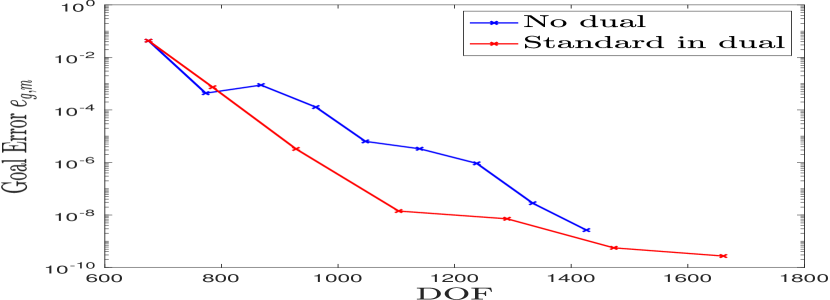
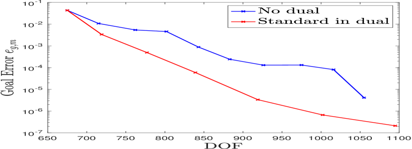
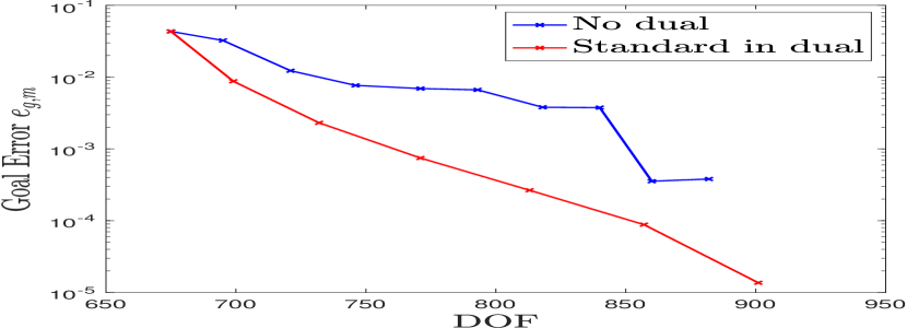
First, we apply the standard enrichment proposed in Section 4.1 and compute the goal error $e_{g,m}$. In this example, we set the number of initial basis functions $l_{i}=3$ for each coarse neighborhood $\omega_{i}$. The results are presented in Figure 2. For instance, the blue curve in Figure 2(a) refers the goal-error obtained by using the residual-driven based enrichment of [8] with $\theta=1$. The red curve in Figure 2(b) is the result obtained by the standard enrichment with $\theta=1$ and $\gamma=0.8$. Figure 2(b) shows $\theta=\gamma=0.8$, Figure 2(c) shows $\theta=\gamma=0.5$ and Figure 2(d) shows $\theta=\gamma=0.3$.

From the results of Figure 2(a), the goal-error reduction obtained by the standard enrichment behaves similarly to the example with only primal enrichment. With parameters $\theta=1$ and $\gamma=0.8$, both standard and primal-only enrichment strategies include all the primal online basis functions computed at each stage. In this setting the additional dual basis functions add only a modest amount of stability to the error reduction. However, when the parameters $\theta$ and $\gamma$ are relatively small, the error reduction curve for the standard enrichment using primal and dual online basis functions is noticeably steeper hence more effective than the primal-only enrichment strategy.

(a) $\theta=1$, $\gamma=0.8$

(b) $\theta=\gamma=0.8$.

(c) $\theta=\gamma=0.5$.

(d) $\theta=\gamma=0.3$.

Figure 2: Goal error reduction against DOF. ($l_{i}=3$)

5.2 Example 2: Verification of enrichment strategies

In this example, we investigate the performance of different online enrichments proposed in Section 4. Here, we use the permeability field shown in Figure 1(a) and set $l_{i}=3$. The goal functional in this example is given by (27).

5.2.1 Comparison with the residual-driven approach

First, we compare the efficiency of each dual online enrichment strategy (primial-dual combined and proimal-dual product based) with the primal-only residual-driven approach of [8]. The parameters are set to $\theta=\beta=\tau=0.6$. The convergence history of goal-error using different approaches is shown in Table 1. The profiles of fine-scale solution $u$, multiscale solution $u_{ms}^{m}$ ($m=5$) obtained by primal-dual combined approach, and their difference are sketched in Figure 3.

One may observe that both primal-dual online enrichments outperform the primal residual-driven based approach in terms of the reduction in the goal-error. In particular, both enrichment strategies that incorporate the dual information drive the error decay to a certain range (e.g. $10^{-5}\sim 10^{-4}$) with fewer iterations than the residual-driven approach does. In the meantime, the primal-dual product based strategy in Section 4.3 provides the greatest change in goal-error reduction on the first iteration, while the primal-dual combined algorithm in Section 4.2 shows a greater decrease in error-reduction with fewer DOF as the simulation progresses.

$m$	DOF	$e_{g,m}$
$0$	$675$	$0.0433$
$1$	$732$	$0.0101$
$2$	$782$	$0.0055$
$3$	$842$	$0.0014$
$4$	$894$	$1.48\times 10^{-4}$
$5$	$940$	$2.99\times 10^{-5}$

(a) $\theta=0.6$

$m$	DOF	$e_{g,m}$
$0$	$675$	$0.0433$
$1$	$714$	$0.0105$
$2$	$785$	$6.61\times 10^{-4}$
$3$	$869$	$7.88\times 10^{-5}$
$4$	$957$	$9.05\times 10^{-7}$
$5$	$1058$	$2.23\times 10^{-7}$

(b) $\beta=0.6$

$m$	DOF	$e_{g,m}$
$0$	$675$	$0.0433$
$1$	$745$	$0.0049$
$2$	$867$	$5.41\times 10^{-4}$
$3$	$969$	$7.32\times 10^{-5}$
$4$	$1075$	$9.53\times 10^{-6}$
$5$	$1187$	$6.15\times 10^{-7}$

(c) $\tau=0.6$

Table 1: Results of $e_{g,m}$. Left: primal-only enrichment. Middle: primal-dual combined. Right: primal-dual product.

(a) Fine-scale solution $u$.

(b) Approximation $u_{ms}^{m}$.

(c) Difference $\lvert u-u_{ms}^{m}\rvert$.

Figure 3: Solution profiles of Example 5.2. ($m=5$ using primal-dual combined)

5.2.2 Comparison in dual online enrichments

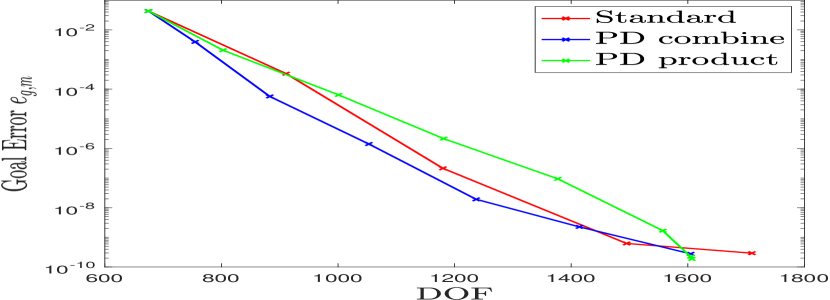
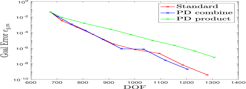
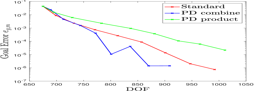
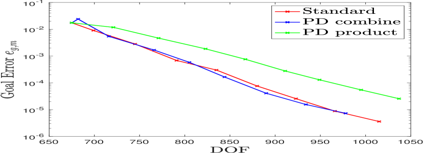
Next, we test the different online enrichments involving the dual problem with different settings of the parameters for adaptivity. The corresponding error reduction in the goal functional for each are shown in Figure 4. As seen in Figures 4(a) with $\theta=1$ and $\gamma=\beta=\tau=0.8$; 4(b) with $\theta=\gamma=\beta=\tau=0.8$; 4(c) with $\theta=\gamma=\beta=\tau=0.5$; and 4(d) with $\theta=\gamma=\beta=\tau=0.3$, the standard and primal-dual combined approaches in Sections 4.1-4.2 yield the best performance with fewer DOF and higher accuracy in terms of goal-error. Overall, Figures 4(a)- 4(d) show the primal-dual combined and standard approaches to have comparable efficiency on each of the problems, although each displays different curves of error reduction suggesting different enrichment in each algorithm. The primal-dual product based enrichment in Section 4.3 based on the error bound (25) as opposed to the online-error reduction prediction (24) gives stable error reduction but with a slower convergence rate.

(a) $\theta=1$, $\gamma=\beta=\tau=0.8$.

(b) $\theta=\gamma=\beta=\tau=0.8$.

(c) $\theta=\gamma=\beta=\tau=0.5$.

(d) $\theta=\gamma=\beta=\tau=0.3$.

Figure 4: Comparing different online enrichments. ($l_{i}=3$)

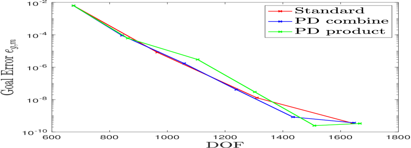
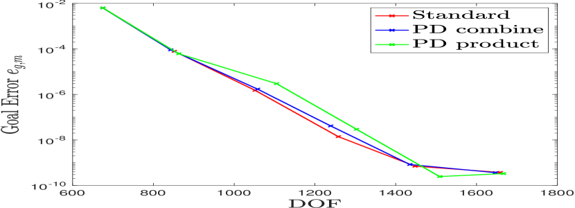
Furthermore, we test the performance of different online enrichments with another specific goal functional, whose effective region is near the middle channel of the permeability field (cf. Figure 1(a), red square). The goal functional $g$ is now given by

$$g(v):=\int_{\widehat{K}}v(x)\leavevmode\nobreak\ dx,\quad\widehat{K}:=[1/2,9/16]\times[7/16,1/2].$$

We keep the source function $f$ and the permeability field $\kappa$ unchanged. Figure 5 records the results of $e_{g,m}$ obtained by using different online enrichments with varying setting of adaptive parameters. Again one may observe that both the standard and primal-dual combined enrichments give a faster convergence rate than does the primal-dual product based approach, especially when the parameters getting small (cf. Figures 5(c) and 5(d)).

Remark.

The results in this example also indicate that the bound (20) which motivates both standard and combined enrichment strategies provide a better indication of the role of online basis functions in goal-error reduction than does (25) which shows the reliability of the product-based estimator. Similarly to how the primal-only strategy can work, but is less effective than the primal-dual strategies; the indicator shown effective for primal-dual offline enrichment also can work, but is also less effective than the online-specific primal-dual strategies.

(a) $\theta=1$, $\gamma=\beta=\tau=0.8$.

(b) $\theta=\gamma=\beta=\tau=0.8$.

(c) $\theta=\gamma=\beta=\tau=0.5$.

(d) $\theta=\gamma=\beta=\tau=0.3$.

Figure 5: Comparing different online enrichments with another $g$. ($l_{i}=3$)

5.3 Example 3: Discussion of ONERP

In the section, we discuss how ONERP effects the performance of the dual online algorithms for a given goal functional. In this example, we keep the source function unchanged and use a different permeability field $\kappa$. Set the goal functional $g:V\to\mathbb{R}$ to be

$$g(v):=-\int_{\widetilde{K}}v(x)\ dx,\quad\widetilde{K}=[3/8,7/16]\times[3/4,13/16].$$ (28)

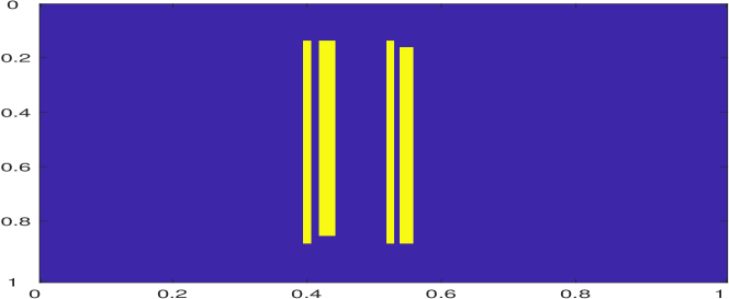
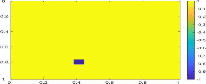
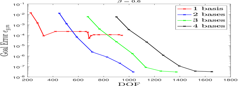
See Figure 6 for the visualizations of the indicator function of $\widetilde{K}$ and the permeability field $\kappa$. We test the cases of different contrast values over the channels (i.e. the yellow region in Figure 6(a)). In particular, we increase the contrast by a factor of 100 to see if there are changes in the convergence behavior. In the high-contrast case, the first few eigenvalues related to the channel regions become 100 times smaller [12], meaning an increased number of offline basis functions are necessary for the error bound (24) to assure rapid convergence. Our numerical results illustrate this requirement, as convergence of the error is seen with only a single basis function per neighborhood in the lower-contrast case but not in the higher-contrast case.

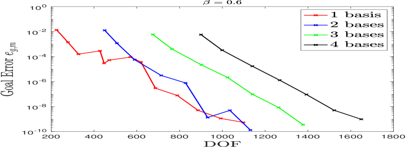
Next, we present the error reduction in the primal-dual combined enrichment resulting from different numbers of initial basis functions in the offline space. Here, the parameter is $\beta=0.6$. The results are in Figure 7. In the lower contrast case, the smallest eigenvalue whose eigenvector is not included in the offline space is 47.5389 when $l_{i}=1$. However, in the high contrast case, the corresponding eigenvalue is only 0.4759, meaning the ONERP is not satisfied. As shown in Figure 7(b), when only 1 initial basis function is used in each coarse neighborhood, the goal-error decay becomes slower compared to the lower contrast case, and indeed convergence is not observed. The goal-error in this case $e_{g,m}$ stalls at the level around $10^{-4}$. However, when sufficiently many (in this case, two or three) initial (local) basis functions are included in the offline space $V_{\text{off}}$, then the rate of error decay is independent of the contrast of the permeability field.

We remark that for the lower contrast case the goal-error is still reduced (with the least stability and more iterations) to below $10^{-8}$ when only a single offline basis function used in each coarse neighborhood (see red curve in Figure 7(a)).

(a) Permeability field $\kappa$.

(b) Function $\mathbf{1}_{\widetilde{K}}$.

Figure 6: Numerical setting of Example 5.3.

(a) Contrast: $1e4$.

(b) Contrast: $1e6$.

Figure 7: Goal-error reduction using primal-dual combined approach.

6 Conclusion

In this research, we propose a GMsFEM based goal-oriented online adaptivity framework for approximating quantities of interest for flow in heterogeneous media. The main idea of the method involves constructing both primal and dual online basis functions by solving local problems related to the local residuals. Each primal (respectively dual) online basis function is computed by solving a local problem for the Riesz representative of the current primal (respectively dual) residual in each coarse neighborhood. After the online basis functions are constructed, they are used to enrich the multiscale space in the next level of the adaptive algorithm to improve the accuracy in a low-dimensional approximation of the quantity of interest. The convergence analysis of the method shows a guaranteed rate of error reduction so long as sufficiently many offline basis functions are used to form the initial multiscale space.

The numerical results support the analysis and demonstrate the necessity of the dual basis functions for efficient error reduction in the quantity of interest. Three online enrichment strategies are proposed to adaptively select which regions are supplemented with the online basis functions. While the primal residual based approach is seen to provide a slower and less stable rate of error reduction, particularly for lower values of the adaptivity parameters, the online-specific primal-dual approaches each succeed in achieving steady and more efficient rates. A comparison between different dual strategies is made and the standard approach and primal-dual combined strategies are seen to be the most stable and efficient over different settings of the adaptivity parameters. With sufficiently many basis functions included in the initial offline space, a steady rate of error reduction is observed in the primal-dual standard and combined strategies independent of the contrast in the permeability field.

Acknowledgement

EC’s work is partially supported by Hong Kong RGC General Research Fund (Project 14304217) and CUHK Direct Grant for Research 2017-18. SP was supported in part by NSF DMS 1719849 and NSF DMS 1852876.

References

- [1] M. Ainsworth and J. T. Oden. A posteriori error estimation in finite element analysis. Pure and Applied Mathematics. New York : John Wiley, 2000.
- [2] M. Arndt and M. Luskin. Goal-oriented atomistic-continuum adaptivity for the quasicontinuum approximation. International Journal for Multiscale Computational Engineering, 5(5), 2007.
- [3] P. T. Bauman, J. T. Oden, and S. Prudhomme. Adaptive multiscale modeling of polymeric materials with arlequin coupling and goals algorithms. Computer Methods in Applied Mechanics and Engineering, 198(5-8):799–818, 2009.
- [4] R. Becker and R. Rannacher. An optimal control approach to a posteriori error estimation in finite element methods. Acta Numer., 10:1–102, 2001.
- [5] N. Castelletto, H. Hajibeygi, and H. A. Tchelepi. Multiscale finite-element method for linear elastic geomechanics. Journal of Computational Physics, 331:337–356, 2017.
- [6] Z. Chen and T. Y. Hou. A mixed multiscale finite element method for elliptic problems with oscillating coefficients. Mathematics of Computation, 72(242):541–576, 2003.
- [7] E. T. Chung, Y. Efendiev, and T. Y. Hou. Adaptive multiscale model reduction with generalized multiscale finite element methods. Journal of Computational Physics, 320:69–95, 2016.
- [8] E. T. Chung, Y. Efendiev, and W. T. Leung. Residual-driven online generalized multiscale finite element methods. Journal of Computational Physics, 302:176–190, 2015.
- [9] E. T. Chung, Y. Efendiev, and G. Li. An adaptive GMsFEM for high-contrast flow problems. Journal of Computational Physics, 273:54–76, 2014.
- [10] E. T. Chung, W. T. Leung, and S. Pollock. Goal-oriented adaptivity for GMsFEM. Journal of Computational and Applied Mathematics, 296:625–637, 2016.
- [11] E. T. Chung, S. Pollock, and S.-M. Pun. Goal-oriented adaptivity of mixed GMsFEM for flows in heterogeneous media. Comput. Methods Appl. Mech. and Eng., 323:151 – 173, 2017.
- [12] Y. Efendiev and J. Galvis. A domain decomposition preconditioner for multiscale high-contrast problems. In Domain Decomposition Methods in Science and Engineering XIX, pages 189–196. Springer, 2011.
- [13] Y. Efendiev and J. Galvis. Coarse-grid multiscale model reduction techniques for flows in heterogeneous media and applications. Chapter of Numerical Analysis of Multiscale Problems, Lecture Notes in Computational Science and Engineering, Vol. 83., pages 97–125, 2012.
- [14] Y. Efendiev, J. Galvis, and T. Y. Hou. Generalized multiscale finite element methods (GMsFEM). Journal of Computational Physics, 251:116–135, 2013.
- [15] Y. Efendiev, J. Galvis, G. Li, and M. Presho. Generalized multiscale finite element methods: Oversampling strategies. International Journal for Multiscale Computational Engineering, 12(6), 2014.
- [16] Y. Efendiev, J. Galvis, and X.-H. Wu. Multiscale finite element methods for high-contrast problems using local spectral basis functions. Journal of Computational Physics, 230(4):937–955, 2011.
- [17] Y. Efendiev and A. Pankov. Numerical homogenization of nonlinear random parabolic operators. Multiscale Modeling & Simulation, 2(2):237–268, 2004.
- [18] B. Engquist and P. E. Souganidis. Asymptotic and numerical homogenization. Acta Numerica, 17:147–190, 2008.
- [19] M. Feischl, D. Praetorius, and K. G. van der Zee. An abstract analysis of optimal goal-oriented adaptivity. SIAM J. Numer. Anal., 54(3):1423–1448, 2016.
- [20] J. Galvis and Y. Efendiev. Domain decomposition preconditioners for multiscale flows in high-contrast media. Multiscale Modeling & Simulation, 8(4):1461–1483, 2010.
- [21] M. Holst and S. Pollock. Convergence of goal oriented methods for nonsymmetric problems. Numer. Meth. Part. D.E., 32(2):479–509, 2016.
- [22] T. Y. Hou and X.-H. Wu. A multiscale finite element method for elliptic problems in composite materials and porous media. Journal of Computational Physics, 134(1):169–189, 1997.
- [23] C. Jhurani and L. Demkowicz. Multiscale modeling using goal-oriented adaptivity and numerical homogenization. Part I: Mathematical formulation and numerical results. Computer Methods in Applied Mechanics and Engineering, 213:399–417, 2012.
- [24] F. Legoll and L. Chamoin. Multiscale computations based on msfem: model reduction and goal-oriented a posteriori error estimation. In 8th International Conference on Adaptive Modeling and Simulation-ADMOS 2017, 2017.
- [25] A. Loseille, A. Dervieux, and F. Alauzet. Fully anisotropic goal-oriented mesh adaptation for 3D steady Euler equations. Journal of Computational Physics, 229(8):2866–2897, 2010.
- [26] M. S. Mommer and R. Stevenson. A goal-oriented adaptive finite element method with convergence rates. SIAM J. Numer. Anal., 47(2):861–886, 2009.
- [27] I. Niyonzima, C. Geuzaine, and S. Schöps. Waveform relaxation for the computational homogenization of multiscale magnetoquasistatic problems. Journal of Computational Physics, 327:416–433, 2016.
- [28] J. T. Oden and S. Prudhomme. Estimation of modeling error in computational mechanics. Journal of Computational Physics, 182(2):496–515, 2002.
- [29] J. T. Oden, S. Prudhomme, A. Romkes, and P. T. Bauman. Multiscale modeling of physical phenomena: Adaptive control of models. SIAM Journal on Scientific Computing, 28(6):2359–2389, 2006.
- [30] J. T. Oden and K. S. Vemaganti. Estimation of local modeling error and goal-oriented adaptive modeling of heterogeneous materials: I. error estimates and adaptive algorithms. Journal of Computational Physics, 164(1):22–47, 2000.
- [31] F. Otero, S. Oller, X. Martinez, and O. Salomón. Numerical homogenization for composite materials analysis. comparison with other micro mechanical formulations. Composite Structures, 122:405–416, 2015.
- [32] H. Owhadi. Bayesian numerical homogenization. Multiscale Modeling & Simulation, 13(3):812–828, 2015.
- [33] P. J. Park and T. Y. Hou. Multiscale numerical methods for singularly perturbed convection-diffusion equations. International Journal of Computational Methods, 1(01):17–65, 2004.
- [34] D. Peterseim. Variational multiscale stabilization and the exponential decay of fine-scale correctors. In Building bridges: connections and challenges in modern approaches to numerical partial differential equations, pages 343–369. Springer, 2016.
- [35] Y. Wang and J. C. Ragusa. Standard and goal-oriented adaptive mesh refinement applied to radiation transport on 2D unstructured triangular meshes. Journal of Computational Physics, 230(3):763–788, 2011.