Direct numerical simulations of Taylor–Couette turbulence: the effect of sand grain roughness
Abstract
Progress in roughness research, mapping any given roughness geometry to its fluid dynamic behaviour, has been hampered by the lack of accurate and direct measurements of skin-friction drag, especially in open systems. The Taylor–Couette (TC) system has the benefit of being a closed system, but its potential for characterizing irregular, realistic, 3-D roughness has not been previously considered in depth.
Here, we present direct numerical simulations (DNSs) of TC turbulence with sand grain roughness mounted on the inner cylinder. The model proposed by Scotti (Phys. Fluids, vol. 18, 031701, 2006) has been improved to simulate a random rough surface of monodisperse sand grains, which is characterized by the equivalent sand grain height . Taylor numbers range from (corresponding to ) to (). We focus on the influence of the roughness height in the transitionally rough regime, through simulations of TC with rough surfaces, ranging from up to , where the superscript ‘’ indicates non-dimensionalization in viscous units.
We analyse the global response of the system, expressed both by the dimensionless angular velocity transport and by the friction factor . An increase in friction with increasing roughness height is accompanied with enhanced plume ejection from the inner cylinder. Subsequently, we investigate the local response of the fluid flow over the rough surface. The equivalent sand grain roughness is calculated to be , where is the size of the sand grains. We find that the downwards shift of the logarithmic layer, due to transitionally rough sand grains exhibits remarkably similar behavior to that of the Nikuradse (VDI-Forschungsheft 361, 1933) data of sand grain roughness in pipe flow, regardless of the Taylor number dependent constants of the logarithmic layer.
1 Introduction
Many turbulent flows in nature and industry are bounded by rough boundaries. Examples are the surface of the planet with respect to geophysical flows or fouling on ship hulls with respect to open waters. Such rough boundaries strongly influence the total drag, with often adverse consequences in the form of higher transport costs. Therefore, it becomes of paramount importance to understand the physics behind such changes in drag, ultimately leading to better informed management of the problem. One key recurring question concerns the influence of the roughness topology on the drag coefficient.
Seminal work by Nikuradse (1933) investigated the influence of the height of closely packed, monodisperse, sand grains in pipe flow. This work has become one of the pillars in the field. Later, a vast amount of research was carried out to study the influence of roughness on the canonical systems of turbulence – pipe, channel, and boundary layer flows – aiming for a better understanding of the roughness effects on turbulent flows Ligrani & Moffat (1986); Schultz & Flack (2007); Chan et al. (2015); Busse et al. (2017); also see Jimenez (2004), and Schultz & Flack (2010) for comprehensive reviews.
Next to pipe flow, Taylor–Couette (TC) flow – the flow between two coaxial, independently rotating cylinders – is another canonical system in turbulence (Grossmann et al., 2016). Closely related to its ‘twin’ of Rayleigh–Bénard (RB) turbulence (Busse, 2012; Eckhardt et al., 2007), it serves as an ideal system to study the interaction between boundary layer and bulk flow. Very long spatial transients, as found in open systems, are bypassed by the circumferential restrictions. Since the domain is closed, global balances can be easily derived and monitored, giving room for extensive comparison between theory, experiments and simulations. Further, the streamwise curvature effects find many applications in industry. For these reasons, we set out to investigate the effects of roughness on the turbulent fluid flow in the TC system.
Over the last century, much work has been carried out with the aim of understanding the effect of the roughness topology on fluid flow. One of the consequences of roughness is the change of the wall drag, which can be expressed as a shift of the mean streamwise velocity profile , where is known as the Hama roughness function (Hama, 1954) and are the smooth-wall and the rough-wall mean streamwise velocities, respectively. Clauser (1954) and Hama (1954) already observed that roughness effects are confined to the inner region of the boundary layer. Namely that the velocity deficit occurs in the log layer. Shockling et al. (2006) and Schultz & Flack (2007) later found strong support for this notion. The shift in the mean streamwise velocity profile then becomes (Pope, 2000)
| (1) |
As usual, the superscript ‘+’ indicates a scaling in viscous units (e.g. length and velocity ) and is the friction velocity, with being the total tangential stress at the wall, and the fluid density. Note that in this representation, the skin-friction coefficient is related to the friction velocity by , where is the centerline velocity (Pope, 2000). It has been found that for TC turbulence and are not constant anymore, but are functions of the inner cylinder Reynolds number at least until (Huisman et al., 2013). Therefore, for TC we here suggest the generalization;
| (2) |
with and being unknown functions. The questions now are: How does depend on the parameters that characterize the surface geometry. Can be generalized to other flows.
Although many parameters influence the Hama roughness function (Schlichting, 1936; Musker, 1980; Napoli et al., 2008; Chan et al., 2015; MacDonald et al., 2016), the most relevant parameter is the characteristic height of the roughness . In a regime in which the pressure forces dominate the drag force, any surface can be collapsed onto the Nikuradse data by rescaling the roughness height to the so-called ‘equivalent sandgrain roughness height’ . Nikuradse (1933) found that three regimes of the characteristic roughness height can be differentiated with respect to the effect of roughness (Flack et al., 2012). For , the rough wall appears to be hydrodynamically smooth and the roughness function goes to zero. For , the wall drag scales quadratically with the fluid velocity and the friction factor is independent of the Reynolds number, indicating that hydrodynamic pressure drag (also called form drag) on the roughness dominates the total drag. The transitionally rough regime is in between these two regimes. Where in the fully rough regime, a surface is fully determined by to give a collapse onto the fully rough asymptote (Schultz & Flack, 2010), in the transitionally rough regime, any unique surface corresponds to a unique roughness function. This can be attributed to the delicate interplay between pressure drag, viscous drag, and the weakening of the so-called viscous generation cycle (Jimenez, 2004).
An intriguing feature of the data from Nikuradse (1933) is at , where roughness effects suddenly result in an inflectional increase of , as compared to the gradual increase of the roughness function found by Colebrook (1939) who extracted an empirical relationship from many industrial surfaces (Shockling et al., 2006). Later, this inflectional behavior was also observed for tightly packed spheres (Ligrani & Moffat, 1986), honed surfaces (Shockling et al., 2006), and grit-blasted surfaces (Thakkar et al., 2018). Chan-Braun et al. (2011) had too few points to find the inflectional behavior; however, their two simulations of monodisperse spheres in regular arrangement collapsed on the Nikuradse curve. In the Moody (Moody, 1944) representation, this inflectional behavior manifests itself as a dip in the friction factor , leading to a significantly lower drag coefficient ( (Bradshaw, 2000)) in comparison to the monotonic behavior of Colebrook (1939), on which the original Moody diagram is based. Although it is proposed that the inflectional behavior has to do with the monodispersity of the roughness leading to a critical Reynolds number at which the elements become active (Jimenez, 2004), recent simulations by Thakkar et al. (2018) for a polydisperse surface (containing irregularities with a range of sizes) also show this inflectional behavior. In a broader sense, the DNS by Thakkar et al. (2018) are interesting since they show, for the first time, a surface that very closely and quantitatively resembles the Nikuradse (1933) roughness function in all regimes, the authors found .
Regarding TC flow, only a few studies have looked at the effect of roughness (Cadot et al., 1997; van den Berg et al., 2003). Recently, the effect of regular roughness on TC turbulence has also been investigated by means of DNS (Zhu et al., 2016, 2017, 2018b). Zhu et al. (2016) looked at the effect of axisymmetric grooves on the torque scaling, boundary layer thickness, and plume ejections. They find that enhanced plume ejection from the roughness tips can lead to an ultimate torque scaling exponent of , although for higher the exponent saturates back to the ultimate scaling effective exponent of . Zhu et al. (2017) then simulate transverse bar roughness elements on the inner cylinder to disentangle the separate effects of viscosity and pressure, and find that the ultimate torque scaling exponent of is only possible when the pressure forces dominate at the rough boundary (Zhu et al., 2018b).
In contrast to the above mentioned previous work, in which the roughness consisted of well-defined transverse bars with constant distance and heights (Zhu et al., 2017, 2018b), in this research we set out to investigate the effect of irregular, monodisperse roughness, resembling the sand grain roughness reported by Nikuradse (1933). We model the roughness as randomly rotated and semi-randomly translated ellipsoids of constant volume and aspect ratio, based on the roughness model (subgrid-scale) of Scotti (2006). Previously, a fully resolved version of the model by Scotti (2006) was also used for large-eddy simulations in channel flow (Yuan & Piomelli, 2014). Taylor numbers in our DNS range from () to (); therefore, we capture both classical (laminar-like boundary layers) and ultimate (turbulent boundary layers) regimes (Ostilla-Mónico et al., 2014; Grossmann et al., 2016; Zhu et al., 2018b). Moreover, whereas previous research on roughness in TC flow focussed on the torque scaling, we now look at the effects of the roughness height on the Hama roughness function in the transitionally rough and fully rough regimes, ranging from to .
This manuscript is structured as follows. In §2 & §3, we elaborate on the TC setup, the roughness model and the numerical procedure. In §4.1, we study the velocity profiles and present the effects of the roughness height on the Hama roughness function. In §4.2, we present the global response of the system. In §4.3 we study the flow structures. In §4.4 the fluctuations close to the roughness are studied and in §4.5 we present radial profiles of various other quantities. Finally, in section §5 we draw our conclusions and propose future research directions.
2 Taylor–Couette flow
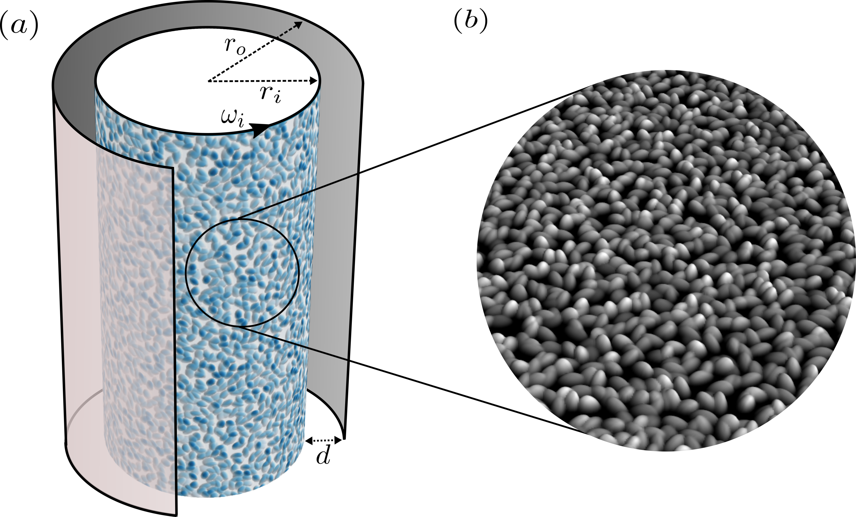
The TC setup, as shown in figure 1, comprises independently co- or counter-rotating concentric cylinders around their vertical axis. The flow, driven by the shear on both of the cylinders, fills the gap between the cylinders. is the inner cylinder radius, is the outer cylinder radius, and the radius ratio is defined as . For this research, we set , in accordance with the experimental T3C setup (Huisman et al., 2013), and previous simulations (Zhu et al., 2017). is the aspect ratio, where is the height of the cylinders, and is the gap width. Here, such that one pair of Taylor vortices fits in the gap, and the mean flow statistics become independent of the aspect ratio (Ostilla-Mónico et al., 2015). In the azimuthal direction we employ a rotational symmetry of order to save on computational expense such that the streamwise aspect ratio of our simulations becomes . Brauckmann & Eckhardt (2013) and Ostilla-Mónico et al. (2015) found that this reduction of the streamwise extent does not effect the mean flow statistics. This gives and .
To maintain convenient boundary conditions, we solve the Navier–Stokes (NS) equations in a reference frame rotating with the inner cylinder () The NS equations in that reference frame become
| (3) |
| (4) |
| (5) |
| (6) |
with no-slip boundary conditions , . Equation (6) expresses the incompressible restriction. Hatted symbols indicate the respective dimensionless variables, with , and . We define where is the so-called ‘geometric Prandtl’ number (Eckhardt et al., 2007):
| (7) |
here and is the Taylor number, which is a measure of the driving strength of the system,
| (8) |
Note that the pressure in the equations above represents the ‘reduced pressure’ that incorporates the centrifugal term; with and is the physical pressure. It is directly clear that the centrifugal force in TC flow is analogous to the gravitational force in RB flow (Eckhardt et al., 2007). The final term on the right-hand side of eq. (3) and (4) gives the Coriolis force, with being the inverse Rossby number
| (9) |
Analogous to RB flow, the global response of TC flow can be expressed in terms of a Nusselt number. In the former, the Nusselt number expresses the dimensionless conserved heat flux, whereas in the latter the Nusselt number expresses the dimensionless conserved angular velocity flux , calculated by:
| (10) |
with the laminar flux given by where is the kinematic viscosity and indicates averaging over the spatial directions , and time . For incompressible flows, it can be derived from the NS equations that is conserved in the radial direction, (Eckhardt et al., 2007). In both cases, the values are made dimensionless by their respective laminar, conducting, values. For TC Nusselt becomes:
| (11) |
The angular velocity flux can easily be written in terms of the torque on any of the cylinders: with being the fluid density. Consequently, the shear stress on the inner cylinder is related to the angular velocity flux by .
Since part of our endeavour is to compare the effects of sand grain roughness on TC turbulence with the effect of sand grain roughness in other canonical systems (e.g. pipe flow), where the use of is not conventional, we choose to also present the global response in terms of the friction factor . Here we follow Lathrop et al. (1992), and define , where is the dimensionless torque and is the inner cylinder Reynolds number . The translation between and is straightforward, namely
| (12) |
Note that one can also define , which is different from eq. (12) by a factor which depends on the radius ratio (Lathrop et al., 1992).
3 Numerical procedure
3.1 Roughness model
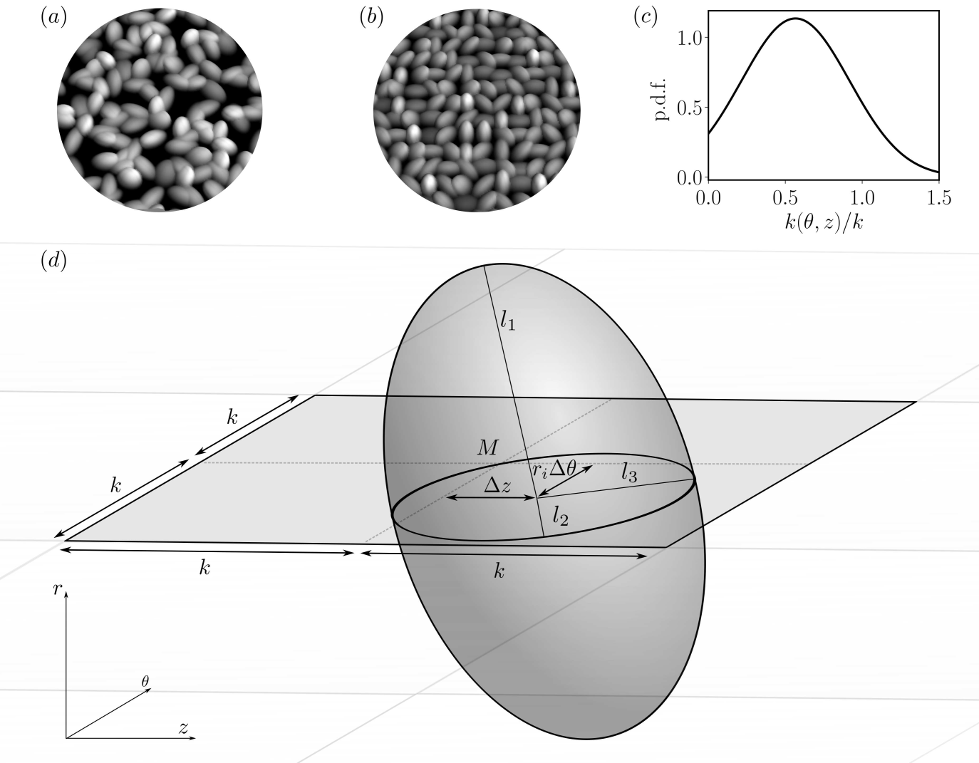
Figure 2 exhibits the setup of the ‘virtual’ sand grain roughness model that is used in this research. The inner cylinder is divided up into square tiles of size , each tile containing exactly ellipsoid. The height is slightly varied () to ensure that an integer amount of tiles fits into the domain. Unlike in the original model by Scotti (2006), we also introduce a random translation of the center of the ellipsoid by applying and , where , and are random uniform translations from the center of the tile. This random translation allows for the surface to be more irregular and as such to relate more closely to a realistic sand grain surface. As also introduced by Scotti (2006), we employ a constant translation of the center of the ellipsoid in the radial direction, with from . It can be seen from figure 1() that part of the cylinder () is not covered by rough elements.
3.2 Numerical method
The NS equations are spatially discretized by using a central second-order finite-difference scheme and solved in cylindrical coordinates by means of a semi-implicit procedure (Verzicco & Orlandi, 1996; van der Poel et al., 2015a). The staggered grid is homogeneous in both the spanwise and streamwise directions (the axial and azimuthal directions respectively).
The wall-normal grid consists of a double cosine (Chebychev-type) grid stretching. Below the maximum roughness height, we employ a cosine stretching such that the maximum grid spacing is always smaller than times the viscous length scale. In the bulk of the fluid, we employ a second stretching, such that the maximum grid spacing in the bulk is approximately times the viscous length scale. The minimum grid spacing is thus located at the position of the maximum roughness height, where we expect the highest shear stress, see table 1 for the exact values.
Time advancement is performed by using a fractional-step third-order Runge–Kutta scheme in combination with a Crank–Nicolson scheme for the implicit terms. The Courant–Friedrichs–Lewy (CFL) () time-step constraint for the non-linear terms is enforced to ensure stability.
Sand grain roughness is implemented in the code by an immersed boundary method (IBM) (Fadlun et al., 2000). In the IBM, the boundary conditions are enforced by adding a body force to the momentum equations (3) - (5). A regular, non-body fitting, mesh can thus be used, even though the rough boundary has a very complex geometry. We perform interpolation in the spatial direction preferentially to the normal surface vector to transfer the boundary conditions to the momentum equations. The IB has been validated previously (Fadlun et al., 2000; Iaccarino & Verzicco, 2003; Stringano et al., 2006; Zhu et al., 2016, 2017, 2018b).
Simulations are run until they become statistically stationary, such that Nusselt number remains constant to within , which requires . Thereafter, we gather statistics until the results converge, which requires . The resolution constraints of the domain are typically derived from the literature and are based on the grid spacing in ‘+’ (viscous) units. Grid independence checks of the time averaged statistics are performed by ensuring that remains constant with increasing grid resolution in all directions and presented along with the results in Table 1.
4 Results
| Case | |||||||||||
| AS | – | – | – | ||||||||
| A1 | |||||||||||
| A2 | |||||||||||
| A3 | |||||||||||
| A4 | |||||||||||
| BS | – | – | – | ||||||||
| B1 | |||||||||||
| B2 | |||||||||||
| B3 | |||||||||||
| BY | |||||||||||
| B4 | |||||||||||
| B5 | |||||||||||
| CS | – | – | – | ||||||||
| C1 | |||||||||||
| C2 | |||||||||||
| C3 | |||||||||||
| C4 | |||||||||||
| CX | |||||||||||
| C5 | |||||||||||
| DS | – | – | – | ||||||||
| D1 | |||||||||||
| D2 | |||||||||||
| D3 | |||||||||||
| D4 | |||||||||||
| D5 |
4.1 Roughness function
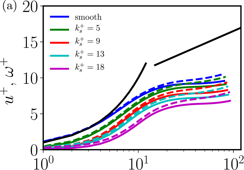
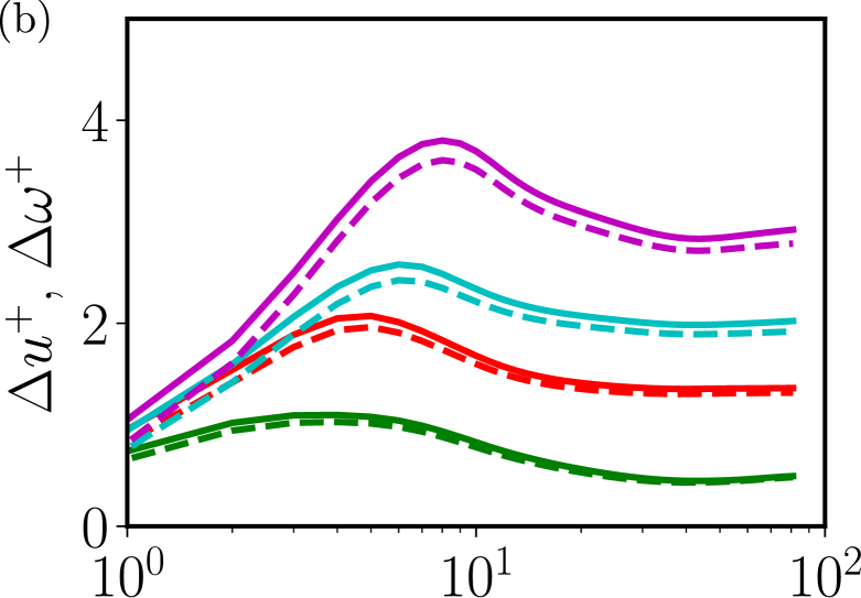
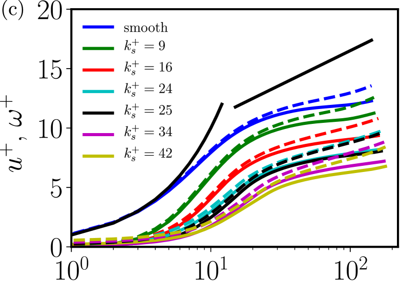
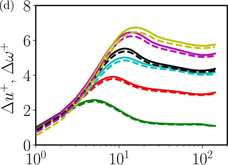
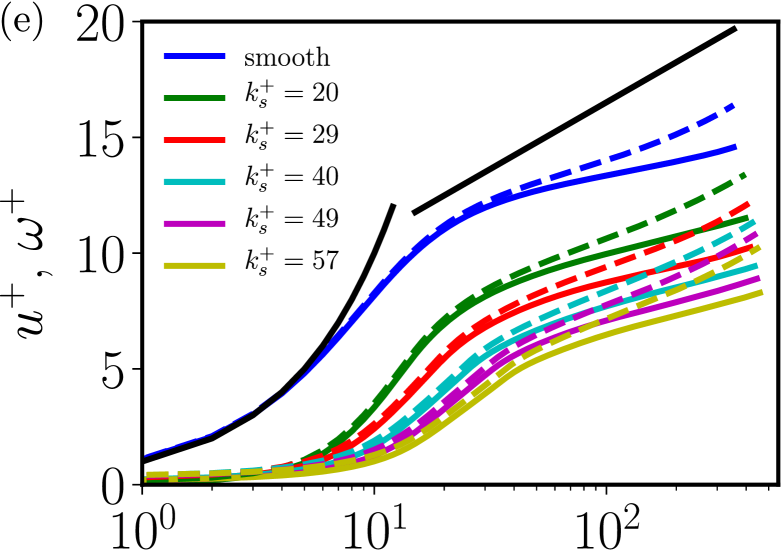
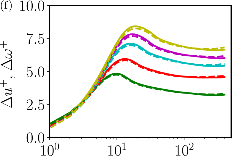
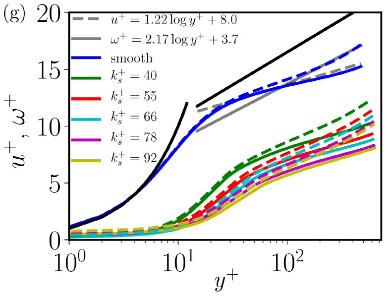
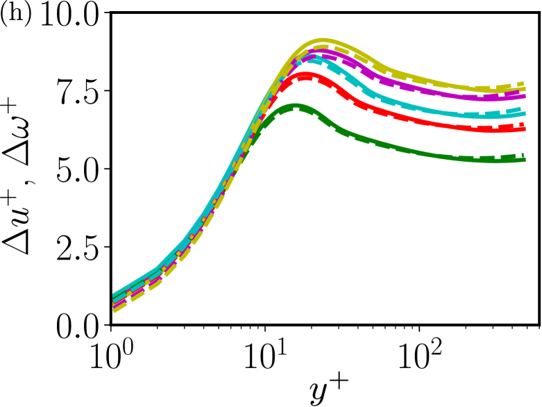
Figure 3 (left column) presents the streamwise (i.e. azimuthal) velocity profiles (solid) and angular velocity profiles (dashed) versus the wall normal distance , where indicates averaging over the streamwise and spanwise directions and in time, and is the mean roughness height. Every row corresponds to simulations at constant rotation rate of the inner cylinder (Taylor number), and increasing roughness height.
In line with the previous observations of Huisman et al. (2013) and Ostilla-Mónico et al. (2014), we also find that the logarithmic profiles of the streamwise velocity in smooth-wall Taylor–Couette do not fit the slope, as found in other wall bounded flows (e.g. pipe, boundary layer, channel) - for similar values of the friction Reynolds number . However, this asymptotic value is experimentally observed at very high shear rates of (Huisman et al., 2013), much higher than can be obtained by the present DNS. The logarithmic profiles of angular velocity have a slope that is closer to the asymptote (Ostilla-Mónico et al., 2015), especially for the higher Ta figure 3(). Here we investigate the effects of roughness on both and .
For rough wall simulations, the logarithmic region shifts downwards - a hallmark effect of a drag increasing surface. Figure 3 (right column) present the shifts, where and . For lower , there is a small but observable difference between and , see figure 3(), whereas for the higher , this difference diminishes, see figure 3().
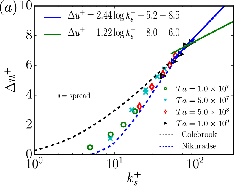
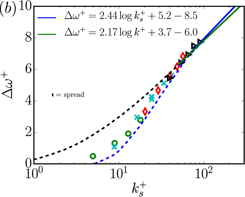
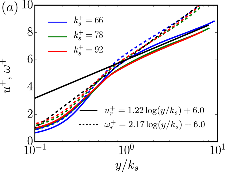
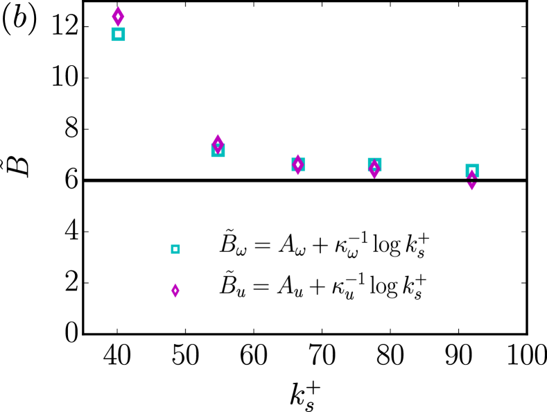
Figure 4() presents the shift of the streamwise and angular velocity profiles, respectively, versus the equivalent roughness height , for all . Care is taken to ensure overlap for varying and similar , to study the dependence of and . However, despite the varying numbers, all data collapse onto a single curve, with some scatter. Note that scatter is expected due to the randomness of the surfaces, which are reproduced for every simulation. To obtain an estimate of the expected scatter, we run two simulations with statistically similar surfaces. These are indicated by B3 and BY in table 1 and the velocity profiles are found in figures 3(). We find a difference between the two cases of .
A comparison with the findings of Nikuradse (1933) can be carried out by scaling the fully rough regime to obtain , where is a constant that depends on the surface topology. In figure 5() we plot the velocity profiles versus for the highest roughness (D3,D4 and D5 respectively, see Table 1). Excellent collapse of the D4 and D5 profiles indicates that those simulations are indeed fully rough. In this fully rough regime viscosity can be neglected (), whereas the velocity profile is also independent of the system outer length scales () i.e. the overlap argument (Pope, 2000). The gradient of the velocity profile becomes; , where is a universal function that will go to . Integration then gives;
| (13) |
where is a constant and . is the Nikuradse constant. The roughness function in the fully rough regime, (i.e. the fully rough asymptote), is obtained by subtracting (13) from the smooth wall profile and rescaling it to overlap with the Nikuradse data:
| (14) |
In figure 4(), the blue solid line is the fully rough asymptote, with as found in pipe flow (Pope, 2000). The green solid line is the fully rough asymptote as obtained from our simulations. and are taken from the fit of the smooth wall simulation at identical as the fully rough cases (figure 3). The fits are in the domain , as there the slope becomes approximately constant (figure 3). is plotted in figure 5(), where we find that for the fully rough cases. The mismatch of the slopes in the fully rough regime makes a rescaling to find a priori impossible - a statement that we wish to emphasize. However, to proceed with the comparison of the transitionally rough cases in TC and pipe flow, we choose to rescale the fully rough cases (D4 and D5) with the Nikuradse fully rough asymptote in figure 4. We find that and very close collapse of our data with the Nikuradse data.
In parallel, we analyse the behavior of versus , shown in figure 4(). Again, the blue solid line represents the fully rough asymptote of Nikuradse. The green solid line is the fully rough asymptote obtained from fits () of the smooth wall angular velocity profile at identical as the fully rough cases, see figure 3(). We find (), close to the asymptotic value . Although the differences are marginally, fits to the Nikuradse data slightly better than (note that also here the rescaling is with the Nikuradse data, ). However, the major difference is the closeness of the fully rough asymptotes.
These results suggest that the near-wall effects of transitionally rough sand grains (and other rough surfaces) in TC flow are similar to the effects of transitionally rough sand grains (and other rough surfaces) in pipe flow (and other canonical systems). Further, we find that these transitionally rough effects are independent of slope of the logarithmic law, whereas in the fully rough regime, they, a priori, depend on this slope. This is confirmed with similar values of at similar , for varying , see figure 4. Also the similarity between and in the transitionally rough regime confirms this, whereas the fully rough asymptotes are very dissimilar. We like to point out that simulations (or experiments) at high enough ( (Huisman et al., 2013)), where , then are expected to also give a collapse to the Nikuradse data in the fully rough regime.
4.2 Global response
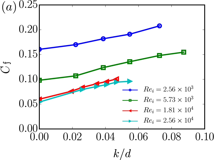
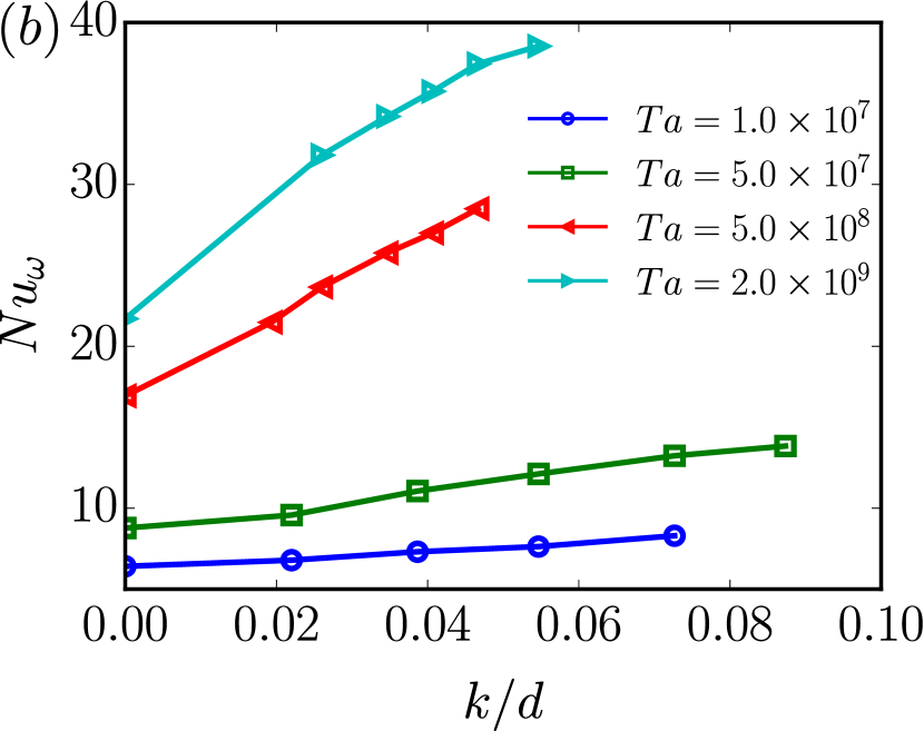
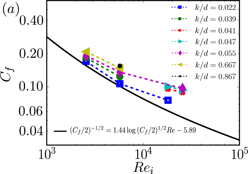
Figure 6() presents the friction factor versus the dimensionless roughness height for varying . For increasing numbers, the friction factor decreases (e.g. figure 7.23 in Pope (2000)), an indication that pressure is not yet dominant. For constant , as expected, the friction factor increases for increasing roughness height. Figure 6() then presents the global response in terms of . We observe an increase in for increasing , corresponding to the increased transport of the angular velocity that is due to the increased turbulent mixing. Higher roughness leads to increased as compared to the smooth wall at the same , which also relates to a higher intensity of the turbulent mixing (the term of equation (10)) and more plumes ejecting from the boundary layer radially outwards (Zhu et al., 2017), on which we will elaborate in §4.3.
By assuming a logarithmic profile, and integrating this profile over the entire gap (thereby neglecting the contributions of the viscous sublayer), we arrive at an implicit equation for the friction factor , namely the celebrated Prandtl’s friction law:
| (15) |
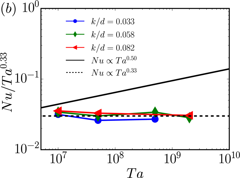
Figure 7 shows the friction factor versus the inner cylinder Reynolds number , for both smooth wall as the rough wall data. An upward shift of the friction factor for increasing roughness height is consistent with what is observed for sand grains in pipe flow (Nikuradse, 1933) and recently also for tranverse ribs in Taylor–Couette flow (Zhu et al., 2018b). Note that this upward shift, is directly related to the downward shift of the mean streamwise velocity profile (the roughness function). Since the friction factor and the Nusselt number are related, as expressed in equation (12), we expect the Nusselt number to increase, for increasing roughness height. This is confirmed in figure 7(), where we plot the Nu number versus the Ta number. The number of simulations with constant is limited, and we vary the Ta number over decades only. However, we clearly observe that the asymptotic, ultimate scaling of , as found for fully rough transverse ribs in (Zhu et al., 2018b), is not reached. This is expected, as for Ta numbers the system is still in the transitionally rough TC regime, where vicous forces still strongly contribute to , and only the inner cylinder is covered with roughness.
4.3 Flow structures
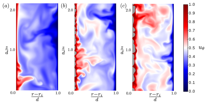
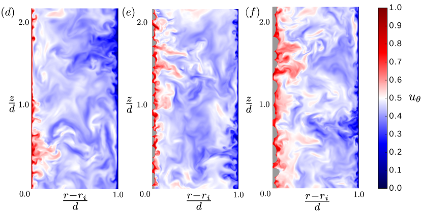
To obtain a qualitative understanding of the effect of inner cylinder roughness on the turbulent flow in the gap, we present two series of snapshots of the streamwise azimuthal velocity . Figure 8() exhibit the snapshots for . It is known, and observed here, that for this Taylor number the coherence length of the dominant flow structures becomes smaller than the gap width , and turbulence develops in the bulk (Grossmann et al., 2016). On the other hand, the boundary layers remain predominantly laminar and as such the regime is referred to as the ‘classical regime’ of TC turbulence. A divergent colormap is chosen to highlight the turbulent structures in the bulk. A snapshot for the smooth inner cylinder simulation is presented in figure 8(). At , one observes an ejecting structure (plume) that detaches from the inner cylinder laminar boundary layer at the location of an adverse pressure gradient. Locally, where this ejecting plume detaches, the flow will be different (i.e. more chaotic) to that in the other parts of the boundary layer. As such, one also expects the local variables (e.g. skin friction, turbulence intensity) to be different. Later we will therefore also employ local averaging, to investigate the spatial differences in the flow associated with this structure (Zhu et al. (2018a); van der Poel et al. (2015b); Ostilla-Mónico et al. (2016)). The ejecting and impacting (located at ) plumes have very strong radial velocity components . From the first term on the right-hand side of (10), , we then directly see that they strongly contribute to . This brings us to the remaining (figure 8 and ) snapshots. Many more, small, plumes are seen to eject from the inner cylinder. The roughness there promotes the detachment of ejecting structures and in that way contributes to a higher . An increase in the level of turbulence, as suggested by the increased level of turbulence dissipation, is quantitatively reflected by a decrease in the Kolmogrov scale (), namely for the smooth wall case BS and for the highest roughness case B5. Note that the decrease in the Kolmogorov scale is only small, since . For TC flow, the volume averaged dissipation rate is related to the angular velocity transport with: , where is the laminar volume averaged dissipation rate, is the gap width of the setup and is a geometric parameter (Eckhardt et al., 2007). As such, we see that only.
Figure 8() presents snapshots of a flow in the ultimate turbulent state at (Grossmann et al., 2016). Although less pronounced than for , we still observe distinct ejecting and impacting regions, indicating the survival of the turbulent Taylor rolls. A similar rationale as applied above, to the classical turbulence case, can also be used to explain the enhancement of the Nusselt number for rough inner cylinders in the ultimate turbulent state. In fact, we can also observe more intense plumes for the highest roughness (D5, figure 8), in comparison to a lower roughness case (D2, figure 8). Note that here we do not observe the stable vortex formation in between roughness elements and the associated ejection of plumes from sharp peaks, as was reported by Zhu et al. (2016) for grooved cylinders, for similar Taylor numbers and roughness heights. The increase in the turbulence level is also quantitatively confirmed by a decrease in the Kolmogorov scale here, for the smooth wall case DS and for the highest roughness case D5.
4.4 Roughness sublayer
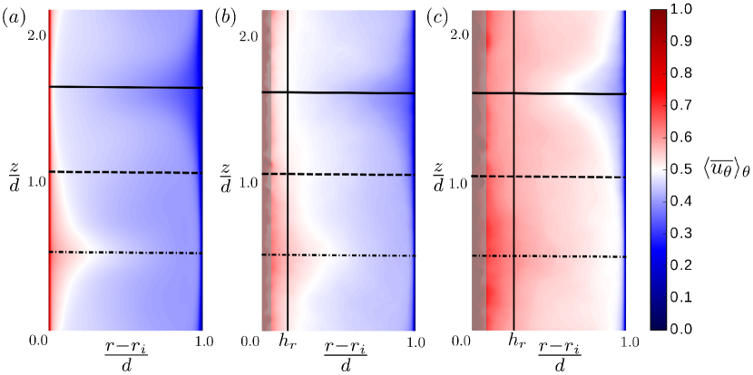
The existence of Taylor roll structures is already anticipated in the snapshots of the instantaneous flow in figure 8, from which we observe the ejecting and impacting plume regions. Contour plots of the time and azimuthally averaged azimuthal velocity field, as presented in figure 9, confirm this. Note that the Taylor roll is spatially fixed, allowing for convenient averaging over impacting (solid line), shearing (dashed line) and ejecting (dashed dotted line) regions, a method that we also have employed in RB flow (van der Poel et al., 2015b). For an increasing roughness height, the white region (representing ) shifts radially outwards and the azimuthal velocity in the bulk increases. This process previously has been seen in Zhu et al. (2018b), where it is referred to as the bulk velocity ‘getting slaved to’ to the velocity of a cylinder covered with roughness, reflecting the enhanced drag on the rough side.
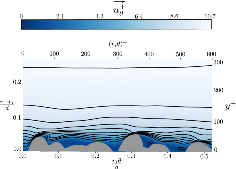
A better impression of the local fluid flow disturbances induced by the roughness elements, is obtained from the time-averaged azimuthal velocity , a contour of which is shown in figure 9. We zoom in on only a few roughness elements and overlay the contour with isolines of . It can quickly be seen that local disturbances are limited to a region of only a few times the roughness height, above which the isolines relax to approximate horizontal lines. Small recirculation zones (closed isolines) are detected in open regions behind high roughness elements. To quantify the degree of roughness-induced velocity disturbances, we apply a triple decomposition to the instanteneous azimuthal velocity (Pokrajac et al., 2007):
| (16) |
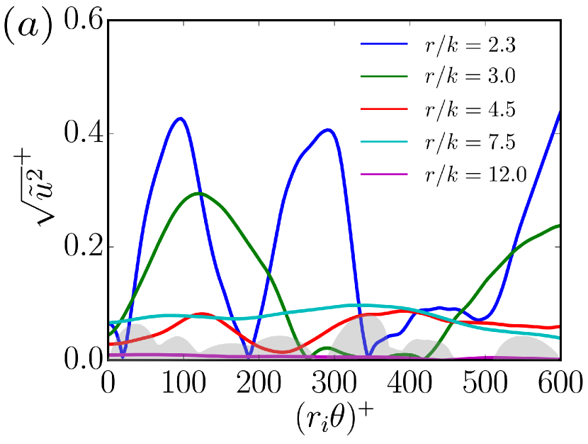
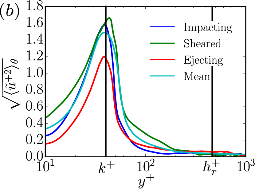
where is the temporal fluctuation and is the component that is strongly related to the roughness induced disturbances and therefore termed the form-induced (or dispersive) velocity fluctuation (for brevity now written as ). Note that by applying the triple decomposition to the full NS equations, one will recover the related form-induced stress tensor . However, here we only discuss . The root mean square of the form-induced fluctuations at various heights above the roughness is given in figure 11(). The horizontal axis corresponds to the roughness elements shown in figure 9. Already for (with being the roughness height) we find it hard to detect spatial fluctuations along . For , the line is barely distinguishable from the horizontal axis. If we average the lines over the azimuthal direction, we obtain the behavior of the dispersive fluctations as a function of the wall normal distance; see figure 11(). We plot the lines for three respective axial locations, that is the impacting, sheared and ejecting regions, and find little variance in the wall normal extent of the form-induced fluctuations, for the varying locations. The vertical black line represent the maximum roughness height, below wich we average only over fluid regions. It is convenient to introduce a height at which dispersive fluctuations vanish, and this height is commonly known as the ‘roughness sublayer height’ . In this research, we define where and find (). This value agrees well with a roughness sublayer height of , as typically found in other canonical flows (Pokrajac et al., 2007).
4.5 Radial profiles
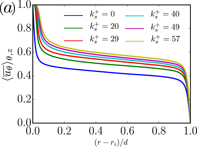
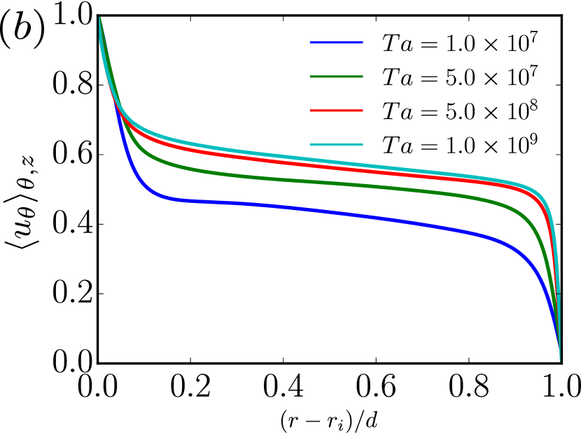
We plot the time and azimuthally averaged azimuthal velocity for in figure 12(). The roughness covers the inner cylinder, i.e. . Below the roughness crest, the velocity is averaged over the entire domain, including the solid rough regions. For increasing roughness height, see the legend for viscous roughness heights, the azimuthal velocity in the bulk increases. Figure 12() then presents the corresponding azimuthal velocity profiles for constant and varying Taylor number.
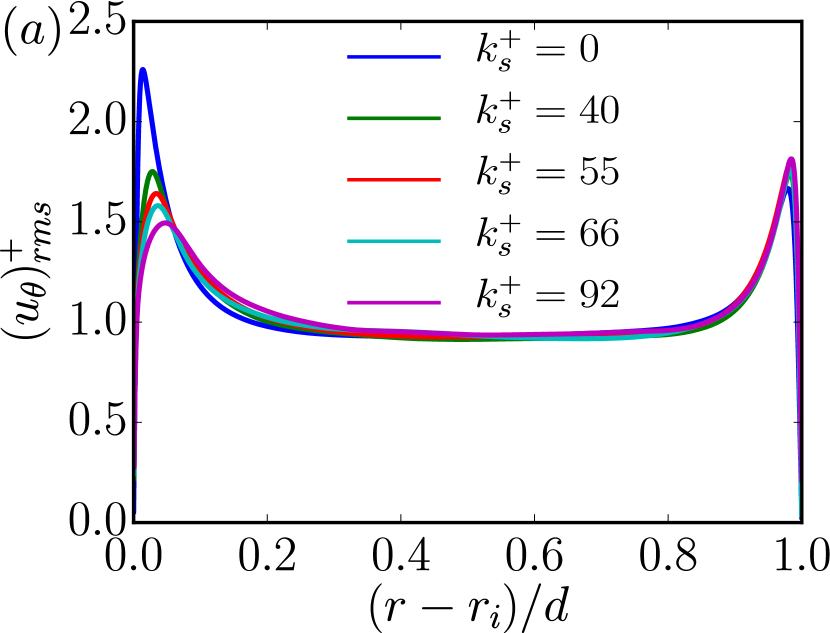
Figure 13() shows the double-averaged radial profiles for constant Taylor number . For the smooth wall case, the peak of the rms of the azimuthal velocity is located at . This agrees with the smooth case in (ostilla16) for TC flow, but is closer to the solid boundary than that is found in channel flow; . We observe a slight decrease in the viscous scaled turbulence intensity for increasing roughness heights, close to the inner cylinder. Further outside the profiles, the profiles collapse. This is once more a sign that the effects of roughness are only confined to the fuid flow close to the wall.
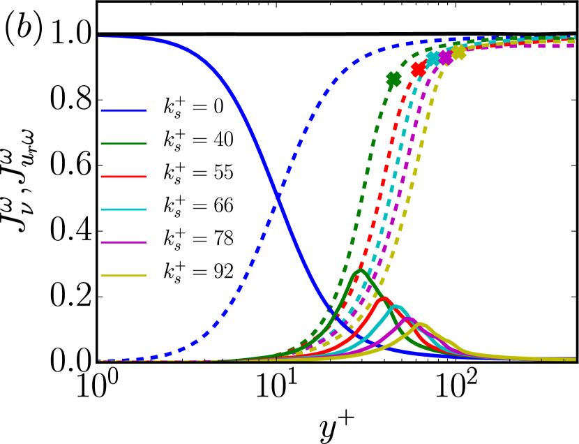
It has already been mentioned that the angular velocity flux is conserved in the radial direction, see section 4.2. However, the individual components – i.e. the viscous and Reynolds stress terms – are functions of the wall normal (radial) coordinate. The profiles of these terms are shown in figure 13(b). We normalize all terms with . The viscous stress terms are presented as solid lines and the Reynolds stress terms as dashed lines. The blue lines represent the smooth wall case. Very close to the inner cyliner (), ; this is expected, since there the gradient of the mean streamwise velocity is maximum and the wall normal component of the velocity vector goes to zero. On the far right of figure 13(b), the gradient of the mean velocity approaches zero in the bulk, and the correlation function between the wall normal and angular velocity goes to a maximum; as such . The black line represents the sum of the viscous and Reynold stress terms, for the smooth (blue) case, and is independent of . The situation for the rough cylinder cases is more complex. For increasing roughness height, the viscous stress reaches a maximum below the maximum roughness height. This can be explained by the recirculation zones behind the roughness elements. Then, above the roughness, the viscous stress goes to zero in the bulk. For the Reynolds stress terms the increase is monotonic, and similar to the smooth wall case. However, we observe a steeper increase for the rough cases. Note that under the maximum roughness height, the viscous and Reynolds stress terms do not add up to unity, since the rough surface acts as a radial dependent momentum source term to the NS equations there.
5 Summary & conclusions
We have performed Direct Numerical Simulations of turbulent Taylor–Couette flow with inner cylinder rotation and inner cylinder sand grain roughness. The Taylor number ranges from () up to (), covering thereby both the classical and the ultimate regimes of turbulent TC flow. In particular, we studied the effects of the roughness height on the fluid flow in the transitionally rough and fully rough regimes, with the equivalent sand grain roughness height ranging from to . We modelled the sand grains as randomly rotated and translated ellipsoids of constant size and shape (monodisperse), similar to the model proposed by Scotti (2006). The surface was implemented into a second order finite difference code by means of the Immersed Boundary Method.
We confirm an increase in the dimensionless torque, expressed as the Nusselt number, for increasing roughness height. This is attributed to the enhanced boundary layer detachment, resulting in plume ejection regions, which we observed in snapshots of the azimuthal velocity field. The plumes contain a strong radial velocity component, and as such contribute strongly to the Reynolds stress term of the angular velocity flux. This mechanism is analogous to what was found for the Nu increase for grooved TC turbulence by Zhu et al. (2016).
To quantify the degree of roughness induced disturbances to the velocity field, we measured the dispersive fluctuations of the azimuthal velocity component, . This dispersive term was obtained by means of a triple decomposition to the azimuthal velocity. We defined the height of the roughness sublayer there where the dispersive fluctuations become very small, such that and found the height of the roughness sublayer to be . This height of the roughness sublayer compares well with values found for other canonical systems (Pokrajac et al., 2007).
The hallmark of turbulent flows over rough walls is the shift of the logarithmic streamwise velocity profile . The shift is a function of any parameters describing the roughness topology. Here we focused in particular on the effect of the sand grain size and the roughness function becomes . It was shown in Huisman et al. (2013) that the constants of the logarithmic law are not constant in the Taylor number range of our simulations. Hence we proposed the generalization; .
We performed simulations at four Ta and various roughness heights and ensured that the range for the various Ta numbers overlaps. First, we concluded that the velocity shift is independent of Ta, despite the Ta dependence of the constant in the logarithmic layer. As such, all simulations collapse onto a single curve. Second, we saw a strong overlap between the roughness function calculated from our DNS in TC flow and the seminal work by Nikuradse (1933) on monodisperse sand grains in pipe flow, in the transitionally rough regime. We found . Only for very low values, close to the hydrodynamically smooth regime, we found that the simulations slightly differ from the Nikuradse curve.
It is remarkable that the Hama roughness function appears to be universal for similar surfaces in such different systems. Note in particular that we have a streamwise curvature and strong secondary motions (Taylor rolls), which were absent in the pipe flow experiments of Nikuradse. As such, our findings point towards a universal behavior of the roughness function for very different fluid flow systems. However, many more comparison studies, of identical rough surfaces and varying fluid flow systems, are needed to confirm this notion.
Acknowledgements
We wish to express our gratitude to Jelle Will for his help with various illustrations. This project is funded by the Priority Programme SPP 1881 Turbulent Superstructures of the Deutsche Forschungsgemeinschaft. We also acknowledge PRACE for awarding us access to Marconi, based in Italy at CINECA under PRACE project number 2016143351. We also acknowledge PRACE for awarding us access to MareNostrum based in Italy at the Barcelona Supercomputing Center (BSC) under PRACE project number 2017174146. This work was partly carried out on the national e-infrastructure of SURFsara, a subsidiary of SURF cooperation, the collaborative ICT organization for Dutch education and research.
Appendix A
| Case | Sk | Ku | ES | |||||||||
|---|---|---|---|---|---|---|---|---|---|---|---|---|
| A1 | ||||||||||||
| A2 | ||||||||||||
| A3 | ||||||||||||
| A4 | ||||||||||||
| B1 | ||||||||||||
| B2 | ||||||||||||
| B3 | ||||||||||||
| BY | ||||||||||||
| B4 | ||||||||||||
| B5 | ||||||||||||
| C1 | ||||||||||||
| C2 | ||||||||||||
| C3 | ||||||||||||
| C4 | ||||||||||||
| C5 | ||||||||||||
| D1 | ||||||||||||
| D2 | ||||||||||||
| D3 | ||||||||||||
| D4 | ||||||||||||
| D5 |
References
- van den Berg et al. (2003) van den Berg, T. H., Doering, C. R., Lohse, D. & Lathrop, D. 2003 Smooth and rough boundaries in turbulent Taylor–Couette flow. Phys. Rev. E 68, 036307.
- Bradshaw (2000) Bradshaw, P. 2000 A note on ‘critical roughness height’ and ‘transitional roughness’. Phys. Fluids 12, 1611.
- Brauckmann & Eckhardt (2013) Brauckmann, Hannes J. & Eckhardt, Bruno 2013 Direct numerical simulations of local and global torque in Taylor-Couette flow up to Re = 30 000. J. Fluid Mech. 718, 398–427.
- Busse et al. (2017) Busse, A., Thakkar, M. & Sandham, N. D. 2017 Reynolds-number dependence of the near-wall flow over irregular rough surfaces. J. Fluid Mech. 810, 196–224.
- Busse (2012) Busse, F. H. 2012 Viewpoint: The twins of turbulence research. Physics 5, 4.
- Cadot et al. (1997) Cadot, O., Couder, Y., Daerr, A., Douady, S. & Tsinober, A. 1997 Energy injection in closed turbulent flows: stirring through boundary layers versus inertial stirring. Phys. Rev. E 56, 427–433.
- Chan et al. (2015) Chan, L., MacDonald, M., Chung, D., Hutchins, N. & Ooi, A. 2015 A systematic investigation of roughness height and wavelength in turbulent pipe flow in the transitionally rough regime. J. Fluid Mech. 771, 743–777.
- Chan-Braun et al. (2011) Chan-Braun, C., Garcia-Villalba, M. & Uhlmann, M. 2011 Force and torque acting on particles in a transitionally rough open-channel flow. J. Fluid Mech. 684, 441–474.
- Clauser (1954) Clauser, F. H. 1954 Turbulent boundary layers in adverse pressure gradients. J. Aeronaut. Sci. 21, 91–108.
- Colebrook (1939) Colebrook, C. F. 1939 Turbulent flow in pipes, with particular reference to the transitional region between smooth and rough wall laws. J. Inst. Civil Engrs 11, 133–156.
- Eckhardt et al. (2007) Eckhardt, B., Grossmann, S. & Lohse, D. 2007 Torque scaling in turbulent Taylor-Couette flow between independently rotating cylinders. J. Fluid Mech. 581, 221–250.
- Fadlun et al. (2000) Fadlun, E.A., Verzicco, R., Orlandi, P. & Mohd-Yusof, J. 2000 Combined immersed-boundary finite-difference methods for three-dimensional complex flow simulations. J. Comput. Phys. 161, 35–60.
- Flack et al. (2012) Flack, K. A., Schultz, M. P. & Rose, W. B. 2012 The onset of roughness effects in the transitionally rough regime. Int. J. Heat Fluid Flow 35, 160–167.
- Grossmann et al. (2016) Grossmann, S., Lohse, D. & Sun, C. 2016 High Reynolds number Taylor-Couette turbulence. Ann. Rev. Fluid Mech 48, 53–80.
- Hama (1954) Hama, F.R. 1954 Boundary-layer characteristics for smooth and rough surfaces. Trans. Soc. Nav. Archit. Mar. Engrs 62, 333–358.
- Huisman et al. (2013) Huisman, S.G., Scharnowski, S., Cierpka, C., Kähler, C.J., Lohse, D. & Sun, C. 2013 Logarithmic boundary layers in strong Taylor-Couette turbulence. Phys. Rev. Lett. 110, 264501.
- Iaccarino & Verzicco (2003) Iaccarino, G. & Verzicco, R. 2003 Immersed boundary technique for turbulent flow simulations. Appl. Mech. Rev. 56, 331–347.
- Jimenez (2004) Jimenez, J. 2004 Turbulent flows of rough walls. Ann. Rev. Fluid Mech. 36, 173–196.
- Lathrop et al. (1992) Lathrop, D P., Fineberg, J. & Swinney, H L. 1992 Transition to shear-driven turbulence in Couette-Taylor flow. Phys. Rev. A 46, 6390–6405.
- Ligrani & Moffat (1986) Ligrani, P. M. & Moffat, R. J. 1986 Structure of transitionally rough and fully rough turbulent boundary layers. J. Fluid Mech. 162, 69–98.
- MacDonald et al. (2016) MacDonald, M., Chan, L., Chung, D., Hutchins, N. & Ooi, A. 2016 Turbulent flow over transitionally rough surfaces with varying roughness densities. J. Fluid Mech. 804, 130–161.
- Moody (1944) Moody, L. F. 1944 Friction factors for pipe flow. Trans. ASME 66, 671–684.
- Musker (1980) Musker, A. J. 1980 Universal roughness functions for naturally-occurring surfaces. Trans. Can. Soc. Mech. Eng. 1, 1–6.
- Napoli et al. (2008) Napoli, E., Armenio, V. & De Marchis, M. 2008 The effect of the slope of irregularly distributed roughness elements on turbulent wall-bounded flows. J. Fluid Mech. 613, 385–394.
- Nikuradse (1933) Nikuradse, J. 1933 Strömungsgesetze in rauhen rohren. VDI-Forschungsheft 361, (English translation – Laws of flow in rough pipes, NACA Technical Memorandum 1292 (1950)).
- Ostilla-Mónico et al. (2014) Ostilla-Mónico, R., van der Poel, E.P., Verzicco, R., Grossmann, S. & Lohse, D. 2014 Boundary layer dynamics at the transition between the classical and the ultimate regime of Taylor-Couette flow. Phys. Fluids 26, 015114.
- Ostilla-Mónico et al. (2016) Ostilla-Mónico, R., Verzicco, R., Grossmann, S. & Lohse, D. 2016 The near-wall region of highly turbulent Taylor–Couette flow. J. Fluid Mech. 788, 95–117.
- Ostilla-Mónico et al. (2015) Ostilla-Mónico, R., Verzicco, R & Lohse, D. 2015 Effects of the computational domain size on direct numerical simulations of Taylor-Couette turbulence with stationary outer cylinder. Phys. Fluids 27, 025110.
- Persson et al. (2005) Persson, B. N. J., Albohr, O., Tartaglino, U., Volokitin, A. I. & Tosatti, E. 2005 On the nature of surface roughness with application to contact mechanics, sealing, rubber, friction and adhesion. J. Phys. Condens. Matter 17, R1.
- van der Poel et al. (2015a) van der Poel, E.P., Ostilla-Mónico, R., Donners, J. & Verzicco, R. 2015a A pencil distributed finite difference code for strongly turbulent wall-bounded flows. Comput. Fluids 116, 10–16.
- van der Poel et al. (2015b) van der Poel, E. P., Ostilla-Mónico, R., Verzicco, R., Grossmann, S. & Lohse, D. 2015b Logarithmic mean temperature profiles and their connection to plume emissions in turbulent Rayleigh–Bénard convection. Phys. Rev. Lett. 115, 154501.
- Pokrajac et al. (2007) Pokrajac, D., Campbell, J. L., Nikora, V., Manes, C. & McEwan, I. 2007 Quadrant analysis of persistent spatial velocity perturbations over square-bar roughness. Exp. Fluids 42, 413–423.
- Pope (2000) Pope, S. B. 2000 Turbulent Flow. Cambridge: Cambridge University Press.
- Schlichting (1936) Schlichting, H. 1936 Experimentelle untersuchungen zum rauigkeitsproblem. Ing. Arch. 36(1), 173–196.
- Schultz & Flack (2007) Schultz, M.P. & Flack, K.A. 2007 The rough-wall turbulent boundary layer from the hydraulically smooth to the fully rough regime. J. Fluid Mech. 580, 381–405.
- Schultz & Flack (2010) Schultz, M.P. & Flack, K.A. 2010 Review of hydraulic roughness scales in the fully rough regime. ASME. J. Fluids Eng. 132 (1).
- Scotti (2006) Scotti, A. 2006 Direct numerical simulation of turbulent channel flows with boundary roughened with virtual sandpaper. Phys. Fluids 18, 031701.
- Shockling et al. (2006) Shockling, M. A., Allen, J. J. & Smits, A. J. 2006 Roughness effects in turbulent pipe flow. J. Fluid Mech. 564, 267–285.
- Sigal & Danberg (1990) Sigal, A. & Danberg, J. E. 1990 New correlation of roughness density effect on the turbulent boundary layer. AIAA J. 28, 554–556.
- Stringano et al. (2006) Stringano, G., Pascazio, G. & Verzicco, R. 2006 Turbulent thermal convection over grooved plates. J. Fluid Mech. 557, 307–336.
- Thakkar et al. (2018) Thakkar, M., Busse, A. & Sandham, N. D. 2018 Direct numerical simulation of turbulent channel flow over a surrogate for Nikuradse-type roughness. J. Fluid Mech. 837, R1–R11.
- Verzicco & Orlandi (1996) Verzicco, R. & Orlandi, P. 1996 A finite-difference scheme for three-dimensional incompressible flow in cylindrical coordinates. J. Comput. Phys. 123, 402–413.
- van der Walt et al. (2014) van der Walt, J., Schönberger, J.L., Nunez-Iglesias, J., Boulogne, F., Warner, J.D., Yager, N., Gouillart, E., Yu, T. & the scikit-image contributors. 2014 scikit-image: Image processing in Python. PeerJ 2:e453 [Online; accessed December 2017].
- Yuan & Piomelli (2014) Yuan, J. & Piomelli, U. 2014 Roughness effects on the Reynolds stress budgets in near-wall turbulence. J. Fluid Mech. 760, R1–R12.
- Zhu et al. (2018a) Zhu, X., Mathai, V., Stevens, R. J. A. M., Verzicco, R. & Lohse, D. 2018a Transition to the ultimate regime in two-dimensional Rayleigh–Bénard convection. Phys. Rev. Lett. 120, 144502.
- Zhu et al. (2016) Zhu, X., Ostilla-Mónico, R., Verzicco, R & Lohse, D. 2016 Direct numerical simulation of Taylor-Couette flow with grooved walls: torque scaling and flow structure. J. Fluid Mech. 794, 746–774.
- Zhu et al. (2017) Zhu, X., R., Verzicco, R & Lohse, D. 2017 Disentangling the origins of torque enhancement through wall roughness in Taylor-Couette turbulence. J. Fluid Mech. 812, 279–293.
- Zhu et al. (2018b) Zhu, X., Verschoof, R.A., Bakhuis, D., Huisman, S.G., Verzicco, R., Sun, C. & Lohse, D. 2018b Wall roughness induces asymptotic ultimate turbulence. Nature Physics 14, 417–423.