Dynamics Based Privacy Protection for Average Consensus on Directed Graphs

Huan Gao,  and Yongqiang Wang Part of the results was accepted for presentation at 2018 IEEE Conference on Communications and Network Security (CNS) [1]. The work was supported in part by the National Science Foundation under Grant 1824014 and 1738902. Huan Gao and Yongqiang Wang are with the Department of Electrical and Computer Engineering, Clemson University, Clemson, SC 29634, USA {hgao2, yongqiw}@clemson.edu
Abstract

Average consensus is key for distributed networks, with applications ranging from network synchronization, distributed information fusion, decentralized control, to load balancing for parallel processors. Existing average consensus algorithms require each node to exchange explicit state values with its neighbors, which results in the undesirable disclosure of sensitive state information. In this paper, we propose a novel average consensus approach for directed graphs which can protect the privacy of participating nodes’ initial states without the assistance of any trusted third party or data aggregator. By leveraging the inherent robustness of consensus dynamics to embed privacy in random coupling weights between interacting nodes, our proposed approach can guarantee consensus to the exact value without any error. This is in distinct difference from differential-privacy based average consensus approaches which enable privacy through sacrificing accuracy in obtained consensus value. The proposed approach is able to preserve privacy even when multiple honest-but-curious nodes collude with each other. Furthermore, by encrypting exchanged information, the proposed approach can also provide privacy protection against inference by external eavesdroppers wiretapping communication links. Numerical simulations and hardware experiments on Raspberry Pi boards confirm that the algorithm is lightweight in computation and communication.

I Introduction

Achieving average consensus is an important problem in distributed computing. For a distributed network of N𝑁N nodes interacting on a connected graph, average consensus can enable all nodes converge to the average of their initial values through iterations based on local interaction between neighboring nodes.

In recent years, average consensus has been extensively studied in distributed networks. Typical applications include load balancing (with divisible tasks) in parallel computing [2, 3], network synchronization [4], distributed information fusion [5, 6], and decentralized control [7, 8]. To make all nodes converge to the average of their initial values, conventional average consensus algorithms require each node to exchange explicit state values with its neighbors. This leads to the disclosure of sensitive state information, which is undesirable in terms of privacy-preservation. In many collaborative applications such as smart grid, banking or health-care networks, privacy-preservation is crucial for encouraging participation in collaboration because individual nodes tend not to trade privacy for performance [9]. For example, a group of individuals using average consensus to compute a common opinion may want to keep secret their individual personal opinions [10]. Another example is power systems where multiple generators want to reach agreement on cost while keeping their individual generation information private [11]. Furthermore, exchanging information in the unencrypted plaintext form is vulnerable to attackers which try to steal information by hacking into communication links. With the increased number of reported attack events and the growing awareness of security, keeping data encrypted in communications has become the norm in many applications, particularly in many real-time sensing and control systems such as power systems and wireless sensor networks.

To enable privacy-preservation in average consensus, some results have been reported. One commonly used approach is differential privacy from the database literature [12, 13, 14, 15, 16]. However, differential-privacy based approaches do not guarantee the exact average value due to their fundamental trade-off between enabled privacy and computational accuracy [17, 15]. To guarantee computational accuracy, which is extremely important in sensor networks and cyber-physical systems, [18, 19, 20, 21] proposed to inject additive correlated noise to exchanged messages, instead of uncorrelated noise used by differential-privacy. Observability based approaches have also been discussed to protect the privacy of multi-agent networks. The basic idea is to design the interaction topology so as to minimize the observability from a compromised agent, which amounts to minimizing its ability to infer the initial states of other network agents [22, 23]. However, observability based approaches cannot protect the privacy of the direct neighbors of the compromised agent. Moreover, both the correlated-noise based and the observability based approaches are vulnerable to external eavesdroppers who can steal exchanged information by hacking into the communication channels [21]. Recently, the authors in [24] proposed a new privacy-preserving approach to improving resilience to external eavesdroppers by encoding privacy in random coupling weights with the assistance of additive homomorphic encryption. However, all the aforementioned approaches require undirected or directed but balanced interactions and none of them are applicable to directed (potentially unbalanced) graphs due to the difficulties in constructing doubly stochastic weight matrices. It is worth noting that the approaches in [25] and [26] for constructing doubly stochastic weight matrices require each node to explicitly send and reveal its weight and state to neighboring nodes, and hence are inapplicable when privacy preservation is required.

In this paper, we address privacy-preserving average consensus under directed graphs that are not necessarily balanced. Building on the conventional push-sum based consensus algorithm, we enable privacy preservation by judiciously adding randomness in coupling weights and leverage the inherent robustness of push-sum to ensure consensus to the accurate value. The approach can also be easily extended to provide privacy protection against external eavesdroppers through incorporating partially homomorphic encryption. Both numerical simulations and hardware experiments are provided to verify the effectiveness and efficiency of the proposed approach.

II Preliminaries

This section introduces some preliminaries of graph theory, the conventional push-sum algorithm, and the Paillier cryptosystem.

II-A Graph Theory

Consider a network of N𝑁N nodes which is represented by a directed graph 𝒢=(𝒱,)𝒢𝒱\mathcal{G}=(\mathcal{V},\,\mathcal{E}) with node set 𝒱={1,2,,N}𝒱12𝑁\mathcal{V}=\{1,2,\ldots,N\}. 𝒱×𝒱𝒱𝒱\mathcal{E}\subset\mathcal{V}\times\mathcal{V} is the set of edges, whose elements are such that (i,j)𝑖𝑗(i,\,j)\in\mathcal{E} holds if and only if there exists a directed communication link from node j𝑗j to node i𝑖i, i.e., node j𝑗j can send messages to node i𝑖i. For notional convenience, we assume no self edges, i.e., (i,i)𝑖𝑖(i,\,i)\notin\mathcal{E} for all i𝒱𝑖𝒱i\in\mathcal{V}. Each edge (i,j)𝑖𝑗(i,\,j) has an associated weight, pij>0subscript𝑝𝑖𝑗0p_{ij}>0. The out-neighbor set of node i𝑖i, which represents the set of nodes that can receive messages from node i𝑖i, is denoted as 𝒩iout={j𝒱|(j,i)}superscriptsubscript𝒩𝑖𝑜𝑢𝑡conditional-set𝑗𝒱𝑗𝑖\mathcal{N}_{i}^{out}=\{j\in\mathcal{V}\,|\,(j,\,i)\in\mathcal{E}\}. Similarly, the in-neighbor set of node i𝑖i, which represents the set of nodes that can send messages to node i𝑖i, is denoted as 𝒩iin={j𝒱|(i,j)}superscriptsubscript𝒩𝑖𝑖𝑛conditional-set𝑗𝒱𝑖𝑗\mathcal{N}_{i}^{in}=\{j\in\mathcal{V}\,|\,(i,\,j)\in\mathcal{E}\}. From the definitions, it can be obtained that i𝒩jout𝑖superscriptsubscript𝒩𝑗𝑜𝑢𝑡i\in\mathcal{N}_{j}^{out} and j𝒩iin𝑗superscriptsubscript𝒩𝑖𝑖𝑛j\in\mathcal{N}_{i}^{in} are equivalent to each other. Node i𝑖i’s out-degree is denoted as Diout=|𝒩iout|superscriptsubscript𝐷𝑖𝑜𝑢𝑡superscriptsubscript𝒩𝑖𝑜𝑢𝑡D_{i}^{out}=|\mathcal{N}_{i}^{out}| and its in-degree is denoted as Diin=|𝒩iin|superscriptsubscript𝐷𝑖𝑖𝑛superscriptsubscript𝒩𝑖𝑖𝑛D_{i}^{in}=|\mathcal{N}_{i}^{in}|, where |𝒮|𝒮|\mathcal{S}| denotes the cardinality of set 𝒮𝒮\mathcal{S}. In this paper, we focus on strongly connected graphs which are defined as follows:

Definition 1

A directed graph 𝒢𝒢\mathcal{G} is strongly connected if for any i,j𝒱𝑖𝑗𝒱i,j\in\mathcal{V} with ij𝑖𝑗i\neq j, there exists at least one directed path from i𝑖i to j𝑗j in 𝒢𝒢\mathcal{G}, where the directed path respects the direction of the edges.

II-B The Conventional Push-Sum Algorithm

Push-sum was introduced in [27] and [28] to achieve average consensus for nodes interacting on a directed graph that is not necessarily balanced (a balanced graph is a graph that satisfies j𝒩iinpij=j𝒩ioutpjisubscript𝑗superscriptsubscript𝒩𝑖𝑖𝑛subscript𝑝𝑖𝑗subscript𝑗superscriptsubscript𝒩𝑖𝑜𝑢𝑡subscript𝑝𝑗𝑖\sum_{j\in\mathcal{N}_{i}^{in}}p_{ij}=\sum_{j\in\mathcal{N}_{i}^{out}}p_{ji} for all i𝑖i). In the conventional push-sum, N𝑁N nodes interact on a directed graph, with each node having an initial state xi0superscriptsubscript𝑥𝑖0x_{i}^{0} (i=1,2,,N𝑖12𝑁i=1,2,\ldots,N). Denote the average of all initial states as α=j=1Nxj0/N𝛼superscriptsubscript𝑗1𝑁superscriptsubscript𝑥𝑗0𝑁\alpha={\sum_{j=1}^{N}x_{j}^{0}}/N. The push-sum algorithm performs two iterative computations in parallel, and allows each node to asymptotically obtain the exact average of the initial values α𝛼\alpha. The mechanism of the conventional push-sum algorithm is described as follows:

  Algorithm 0: Conventional push-sum algorithm


  1. 1.

    Each node i𝑖i initializes si(0)=xi0subscript𝑠𝑖0superscriptsubscript𝑥𝑖0s_{i}(0)=x_{i}^{0}, wi(0)=1subscript𝑤𝑖01w_{i}(0)=1, and πi(0)=si(0)/wi(0)subscript𝜋𝑖0subscript𝑠𝑖0subscript𝑤𝑖0\pi_{i}(0)=s_{i}(0)/w_{i}(0). The coupling weight pijsubscript𝑝𝑖𝑗p_{ij} associated with edge (i,j)𝑖𝑗(i,\,j) satisfies pij(0,1)subscript𝑝𝑖𝑗01p_{ij}\in(0,1) if j𝒩iin{i}𝑗superscriptsubscript𝒩𝑖𝑖𝑛𝑖j\in\mathcal{N}_{i}^{in}\cup\{i\} holds and pij=0subscript𝑝𝑖𝑗0p_{ij}=0 otherwise. pijsubscript𝑝𝑖𝑗p_{ij} also satisfies i=1Npij=1superscriptsubscript𝑖1𝑁subscript𝑝𝑖𝑗1\sum_{i=1}^{N}p_{ij}=1 for j=1,2,,N𝑗12𝑁j=1,2,\ldots,N.

  2. 2.

    At iteration k𝑘k:

    1. (a)

      Node i𝑖i computes pjisi(k)subscript𝑝𝑗𝑖subscript𝑠𝑖𝑘p_{ji}s_{i}(k) and pjiwi(k)subscript𝑝𝑗𝑖subscript𝑤𝑖𝑘p_{ji}w_{i}(k), and sends them to its out-neighbors j𝒩iout𝑗superscriptsubscript𝒩𝑖𝑜𝑢𝑡j\in\mathcal{N}_{i}^{out}.

    2. (b)

      After receiving pijsj(k)subscript𝑝𝑖𝑗subscript𝑠𝑗𝑘p_{ij}s_{j}(k) and pijwj(k)subscript𝑝𝑖𝑗subscript𝑤𝑗𝑘p_{ij}w_{j}(k) from its in-neighbors j𝒩iin𝑗superscriptsubscript𝒩𝑖𝑖𝑛j\in\mathcal{N}_{i}^{in}, node i𝑖i updates sisubscript𝑠𝑖s_{i} and wisubscript𝑤𝑖w_{i} as follows:

      {si(k+1)=j𝒩iin{i}pijsj(k)wi(k+1)=j𝒩iin{i}pijwj(k)\left\{\begin{aligned} &\ s_{i}(k+1)=\sum_{j\in\mathcal{N}_{i}^{in}\cup\{i\}}p_{ij}s_{j}(k)\\ &\ w_{i}(k+1)=\sum_{j\in\mathcal{N}_{i}^{in}\cup\{i\}}p_{ij}w_{j}(k)\end{aligned}\right. (1)
    3. (c)

      Node i𝑖i computes the estimate as πi(k+1)=si(k+1)/wi(k+1)subscript𝜋𝑖𝑘1subscript𝑠𝑖𝑘1subscript𝑤𝑖𝑘1\pi_{i}(k+1)=s_{i}(k+1)/w_{i}(k+1).


For the sake of notational simplicity, the update rule in (1) can be rewritten in a more compact form as follows:

{𝐬(k+1)=𝐏𝐬(k)𝐰(k+1)=𝐏𝐰(k)\left\{\begin{aligned} &\ \mathbf{s}(k+1)=\mathbf{P}\mathbf{s}(k)\\ &\ \mathbf{w}(k+1)=\mathbf{P}\mathbf{w}(k)\end{aligned}\right. (2)

where 𝐬(k)=[s1(k),s2(k),,sN(k)]T𝐬𝑘superscriptsubscript𝑠1𝑘subscript𝑠2𝑘subscript𝑠𝑁𝑘𝑇\mathbf{s}(k)=[s_{1}(k),s_{2}(k),\ldots,s_{N}(k)]^{T} and 𝐰(k)=[w1(k),w2(k),,wN(k)]T𝐰𝑘superscriptsubscript𝑤1𝑘subscript𝑤2𝑘subscript𝑤𝑁𝑘𝑇\mathbf{w}(k)=[w_{1}(k),w_{2}(k),\ldots,w_{N}(k)]^{T}, and 𝐏=[pij]𝐏delimited-[]subscript𝑝𝑖𝑗\mathbf{P}=[p_{ij}] with pijsubscript𝑝𝑖𝑗p_{ij} defined in step 1) of Algorithm 0. According to Algorithm 0, we have 𝐬(0)=[x10,x20,,xN0]T𝐬0superscriptsuperscriptsubscript𝑥10superscriptsubscript𝑥20superscriptsubscript𝑥𝑁0𝑇\mathbf{s}(0)=[x_{1}^{0},x_{2}^{0},\ldots,x_{N}^{0}]^{T} and 𝐰(0)=𝟏𝐰01\mathbf{w}(0)=\mathbf{1}. It is also easy to obtain that matrix 𝐏𝐏\mathbf{P} is column stochastic since its column sums are equal to one, i.e., i=1Npij=1superscriptsubscript𝑖1𝑁subscript𝑝𝑖𝑗1\sum_{i=1}^{N}p_{ij}=1 for j=1,2,,N𝑗12𝑁j=1,2,\ldots,N.

At iteration k𝑘k, each node calculates the ratio πi(k+1)=si(k+1)/wi(k+1)subscript𝜋𝑖𝑘1subscript𝑠𝑖𝑘1subscript𝑤𝑖𝑘1\pi_{i}(k+1)=s_{i}(k+1)/w_{i}(k+1), which is used to estimate the average value α=j=1Nxj0/N𝛼superscriptsubscript𝑗1𝑁superscriptsubscript𝑥𝑗0𝑁\alpha={\sum_{j=1}^{N}x_{j}^{0}}/N. Since the directed graph 𝒢𝒢\mathcal{G} is assumed to be strongly connected, 𝐏ksuperscript𝐏𝑘\mathbf{P}^{k} converges to a rank-111 matrix exponentially fast [29, 30]. Defining 𝐏superscript𝐏\mathbf{P}^{\infty} as the limit of 𝐏ksuperscript𝐏𝑘\mathbf{P}^{k} when k𝑘k\rightarrow\infty, we have that 𝐏superscript𝐏\mathbf{P}^{\infty} is of the form 𝐏=𝐯𝟏Tsuperscript𝐏superscript𝐯𝟏𝑇\mathbf{P}^{\infty}=\mathbf{v}\mathbf{1}^{T} where 𝐯=[v1,v2,,vN]T𝐯superscriptsubscript𝑣1subscript𝑣2subscript𝑣𝑁𝑇\mathbf{v}=[v_{1},v_{2},\ldots,v_{N}]^{T}. Making use of the facts 𝐬(k)=𝐏k𝐬(0)𝐬𝑘superscript𝐏𝑘𝐬0\mathbf{s}(k)=\mathbf{P}^{k}\mathbf{s}(0) and 𝐰(k)=𝐏k𝐰(0)𝐰𝑘superscript𝐏𝑘𝐰0\mathbf{w}(k)=\mathbf{P}^{k}\mathbf{w}(0), we have

πi()=subscript𝜋𝑖absent\displaystyle\pi_{i}(\infty)= si()wi()=[𝐏𝐬(0)]i[𝐏𝐰(0)]i=vij=1Nsj(0)vij=1Nwj(0)subscript𝑠𝑖subscript𝑤𝑖subscriptdelimited-[]superscript𝐏𝐬0𝑖subscriptdelimited-[]superscript𝐏𝐰0𝑖subscript𝑣𝑖superscriptsubscript𝑗1𝑁subscript𝑠𝑗0subscript𝑣𝑖superscriptsubscript𝑗1𝑁subscript𝑤𝑗0\displaystyle\frac{s_{i}(\infty)}{w_{i}(\infty)}=\frac{[\mathbf{P}^{\infty}\mathbf{s}(0)]_{i}}{[\mathbf{P}^{\infty}\mathbf{w}(0)]_{i}}=\frac{v_{i}\sum_{j=1}^{N}s_{j}(0)}{v_{i}\sum_{j=1}^{N}w_{j}(0)} (3)
=\displaystyle= j=1Nxj0N=αsuperscriptsubscript𝑗1𝑁superscriptsubscript𝑥𝑗0𝑁𝛼\displaystyle\frac{\sum_{j=1}^{N}x_{j}^{0}}{N}=\alpha

where [𝐏𝐬(0)]isubscriptdelimited-[]superscript𝐏𝐬0𝑖[\mathbf{P}^{\infty}\mathbf{s}(0)]_{i} and [𝐏𝐰(0)]isubscriptdelimited-[]superscript𝐏𝐰0𝑖[\mathbf{P}^{\infty}\mathbf{w}(0)]_{i} represent the i𝑖i-th element of vectors 𝐏𝐬(0)superscript𝐏𝐬0\mathbf{P}^{\infty}\mathbf{s}(0) and 𝐏𝐰(0)superscript𝐏𝐰0\mathbf{P}^{\infty}\mathbf{w}(0), respectively. Therefore, all estimates π1(k),π2(k),,πN(k)subscript𝜋1𝑘subscript𝜋2𝑘subscript𝜋𝑁𝑘\pi_{1}(k),\pi_{2}(k),\ldots,\pi_{N}(k) asymptotically converge to the average value α=j=1Nxj0/N𝛼superscriptsubscript𝑗1𝑁superscriptsubscript𝑥𝑗0𝑁\alpha={\sum_{j=1}^{N}x_{j}^{0}}/N.

II-C Paillier Cryptosystem

Our method to protect privacy against external eavesdroppers wiretapping communication links is to encrypt exchanged messages. To this end, we combine Paillier cryptosystem [31] with consensus dynamics. The Paillier cryptosystem is a public-key cryptosystem which employs a pair of keys: a public key and a private key (also called secret key). The public key is distributed publicly and can be used by any person to encrypt a message, but such a message can only be decrypted by the private key. Since Paillier cryptosystem does not need the assistance of a trusted third party for key management, it is applicable in open and dynamic networks.

The Paillier cryptosystem includes three algorithms as follows:

  Paillier cryptosystem

  Key generation:

  1. 1.

    Choose two large prime numbers p𝑝p and q𝑞q of equal bit-length and compute n=pq𝑛𝑝𝑞n=pq.

  2. 2.

    Let g=n+1𝑔𝑛1g=n+1.

  3. 3.

    Let λ=ϕ(n)=(p1)(q1)𝜆italic-ϕ𝑛𝑝1𝑞1\lambda=\phi(n)=(p-1)(q-1), where ϕ()italic-ϕ\phi(\cdot) is the Euler’s totient function.

  4. 4.

    Let μ=ϕ(n)1modn𝜇moduloitalic-ϕsuperscript𝑛1𝑛\mu=\phi(n)^{-1}\mod n which is the modular multiplicative inverse of ϕ(n)italic-ϕ𝑛\phi(n).

  5. 5.

    The public key kpsuperscript𝑘𝑝k^{p} for encryption is (n,g)𝑛𝑔(n,g).

  6. 6.

    The private key kssuperscript𝑘𝑠k^{s} for decryption is (λ,μ)𝜆𝜇(\lambda,\mu).

Encryption (c=E(m)𝑐𝐸𝑚c={E}(m)):

Recall the definitions of n={z|z,0z<n}subscript𝑛conditional-set𝑧formulae-sequence𝑧0𝑧𝑛\mathbb{Z}_{n}=\{z\,|\,z\in\mathbb{Z},0\leq z<n\} and n={z|z,0z<n,gcd(z,n)=1}superscriptsubscript𝑛conditional-set𝑧formulae-sequenceformulae-sequence𝑧0𝑧𝑛𝑧𝑛1\mathbb{Z}_{n}^{*}=\{z\,|\,z\in\mathbb{Z},0\leq z<n,\gcd(z,n)=1\} where gcd(a,b)𝑎𝑏\gcd(a,b) is the greatest common divisor of a𝑎a and b𝑏b.

  1. 1.

    Choose a random rn𝑟superscriptsubscript𝑛r\in\mathbb{Z}_{n}^{*}.

  2. 2.

    The ciphertext is given by c=gmrnmodn2𝑐modulosuperscript𝑔𝑚superscript𝑟𝑛superscript𝑛2c=g^{m}\cdot r^{n}\mod n^{2}, where mn,cn2formulae-sequence𝑚subscript𝑛𝑐superscriptsubscriptsuperscript𝑛2m\in\mathbb{Z}_{n},c\in\mathbb{Z}_{n^{2}}^{*}.

Decryption (m=D(c)𝑚𝐷𝑐m={D}(c)):

  1. 1.

    Define the integer division function L(μ)=μ1n𝐿𝜇𝜇1𝑛L(\mu)=\frac{\mu-1}{n}.

  2. 2.

    The plaintext is m=L(cλmodn2)μmodn𝑚modulo𝐿modulosuperscript𝑐𝜆superscript𝑛2𝜇𝑛m=L(c^{\lambda}\mod n^{2})\cdot\mu\mod n.


III The Privacy-Preserving Algorithm and Performance Analysis

In this section, we first show that the conventional push-sum algorithm does not preserve privacy, and then we propose our privacy-preserving average consensus algorithm for directed graphs. To this end, we first introduce the attack model and the definition of privacy.

Definition 2

An honest-but-curious adversary is a node who follows all protocol steps correctly but is curious and collects received data in an attempt to learn the initial value of other participating nodes.

Definition 3

For a distributed network of N𝑁N nodes, the privacy of initial value xi0superscriptsubscript𝑥𝑖0x_{i}^{0} of node i𝑖i is preserved if xi0superscriptsubscript𝑥𝑖0x_{i}^{0} cannot be estimated by honest-but-curious adversaries with any accuracy.

Definition 3 requires that honest-but-curious adversaries cannot even find a range for a private value and thus is more stringent than the privacy definition considered in [32, 33, 34] which defines privacy preservation as the inability of an adversary to uniquely determine the protected value. It is worth noting that by a finite range, we mean lower and upper bounds that an adversary may obtain based on accessible information. We do not consider representation bounds caused by the finite number of bytes that can be used to represent a number in a computer.

We first show that the conventional push-sum algorithm is not privacy-preserving. According to (1) and (2), an honest-but-curious node i𝑖i will receive two messages pijsj(0)subscript𝑝𝑖𝑗subscript𝑠𝑗0p_{ij}s_{j}(0) and pijwj(0)subscript𝑝𝑖𝑗subscript𝑤𝑗0p_{ij}w_{j}(0) from its in-neighbor node j𝒩iin𝑗superscriptsubscript𝒩𝑖𝑖𝑛j\in\mathcal{N}_{i}^{in} after the first iteration k=0𝑘0k=0. Then node i𝑖i can uniquely determine the initial value xj0superscriptsubscript𝑥𝑗0x_{j}^{0} by xj0=sj(0)=pijsj(0)pijwj(0)superscriptsubscript𝑥𝑗0subscript𝑠𝑗0subscript𝑝𝑖𝑗subscript𝑠𝑗0subscript𝑝𝑖𝑗subscript𝑤𝑗0x_{j}^{0}=s_{j}(0)=\frac{p_{ij}s_{j}(0)}{p_{ij}w_{j}(0)} using the fact wj(0)=1subscript𝑤𝑗01w_{j}(0)=1. So an honest-but-curious node can infer the initial values of all its in-neighbors, meaning that the conventional push-sum algorithm cannot provide protection against honest-but-curious attackers.

III-A Privacy-Preserving Average Consensus Algorithm

The above analysis shows that using the same coupling weight pijsubscript𝑝𝑖𝑗p_{ij} for both pijsj(0)subscript𝑝𝑖𝑗subscript𝑠𝑗0p_{ij}s_{j}(0) and pijwj(0)subscript𝑝𝑖𝑗subscript𝑤𝑗0p_{ij}w_{j}(0) leads to the disclosure of the initial state value. Motivated by this observation, we introduce a novel privacy-preserving average consensus algorithm that uses different time-varying coupling weights for sisubscript𝑠𝑖s_{i} and wisubscript𝑤𝑖w_{i} for iterations k=0,,K𝑘0𝐾k=0,\ldots,K, where K𝐾K can be any non-negative integer.

  Algorithm 1: Privacy-preserving average consensus algorithm


  1. 1.

    Positive integer K𝐾K and parameter ε(0, 1)𝜀01\varepsilon\in(0,\,1) are known to every node. Each node i𝑖i initializes si(0)=xi0subscript𝑠𝑖0superscriptsubscript𝑥𝑖0s_{i}(0)=x_{i}^{0}, wi(0)=1subscript𝑤𝑖01w_{i}(0)=1, and πi(0)=si(0)/wi(0)subscript𝜋𝑖0subscript𝑠𝑖0subscript𝑤𝑖0\pi_{i}(0)=s_{i}(0)/w_{i}(0).

  2. 2.

    At iteration k𝑘k:

    1. (a)

      If kK𝑘𝐾k\leq K, node i𝑖i generates one set of random coupling weights {pjis(k)|j𝒩iout{i}}conditional-setsuperscriptsubscript𝑝𝑗𝑖𝑠𝑘𝑗superscriptsubscript𝒩𝑖𝑜𝑢𝑡𝑖\big{\{}p_{ji}^{s}(k)\in\mathbb{R}\,\big{|}\,j\in\mathcal{N}_{i}^{out}\cup\{i\}\big{\}} with the sum of this set equal to 111, and assigns piiw(k)=1superscriptsubscript𝑝𝑖𝑖𝑤𝑘1p_{ii}^{w}(k)=1 and pjiw(k)=0superscriptsubscript𝑝𝑗𝑖𝑤𝑘0p_{ji}^{w}(k)=0 for j𝒩iout𝑗superscriptsubscript𝒩𝑖𝑜𝑢𝑡j\in\mathcal{N}_{i}^{out}; otherwise, node i𝑖i generates one set of random coupling weights {pjis(k)(ε, 1)|j𝒩iout{i}}conditional-setsuperscriptsubscript𝑝𝑗𝑖𝑠𝑘𝜀1𝑗superscriptsubscript𝒩𝑖𝑜𝑢𝑡𝑖\big{\{}p_{ji}^{s}(k)\in(\varepsilon,\,1)\,\big{|}\,j\in\mathcal{N}_{i}^{out}\cup\{i\}\big{\}} satisfying the sum 111 condition, and assigns pjiw(k)=pjis(k)superscriptsubscript𝑝𝑗𝑖𝑤𝑘superscriptsubscript𝑝𝑗𝑖𝑠𝑘p_{ji}^{w}(k)=p_{ji}^{s}(k) for j𝒩iout{i}𝑗superscriptsubscript𝒩𝑖𝑜𝑢𝑡𝑖j\in\mathcal{N}_{i}^{out}\cup\{i\}. For j𝒩iout{i}𝑗superscriptsubscript𝒩𝑖𝑜𝑢𝑡𝑖j\notin\mathcal{N}_{i}^{out}\cup\{i\}, node i𝑖i always sets pjis(k)superscriptsubscript𝑝𝑗𝑖𝑠𝑘p_{ji}^{s}(k) and pjiw(k)superscriptsubscript𝑝𝑗𝑖𝑤𝑘p_{ji}^{w}(k) to 00.

    2. (b)

      Node i𝑖i computes pjis(k)si(k)superscriptsubscript𝑝𝑗𝑖𝑠𝑘subscript𝑠𝑖𝑘p_{ji}^{s}(k)s_{i}(k) and pjiw(k)wi(k)superscriptsubscript𝑝𝑗𝑖𝑤𝑘subscript𝑤𝑖𝑘p_{ji}^{w}(k)w_{i}(k) for j𝒩iout𝑗superscriptsubscript𝒩𝑖𝑜𝑢𝑡j\in\mathcal{N}_{i}^{out}, and sends them to node j𝑗j.

    3. (c)

      After receiving pijs(k)sj(k)superscriptsubscript𝑝𝑖𝑗𝑠𝑘subscript𝑠𝑗𝑘p_{ij}^{s}(k)s_{j}(k) and pijw(k)wj(k)superscriptsubscript𝑝𝑖𝑗𝑤𝑘subscript𝑤𝑗𝑘p_{ij}^{w}(k)w_{j}(k) from its in-neighbors j𝒩iin𝑗superscriptsubscript𝒩𝑖𝑖𝑛j\in\mathcal{N}_{i}^{in}, node i𝑖i updates sisubscript𝑠𝑖s_{i} and wisubscript𝑤𝑖w_{i} in the following way

      {si(k+1)=j𝒩iin{i}pijs(k)sj(k)wi(k+1)=j𝒩iin{i}pijw(k)wj(k)\left\{\begin{aligned} &s_{i}(k+1)=\sum_{j\in\mathcal{N}_{i}^{in}\cup\{i\}}p_{ij}^{s}(k)s_{j}(k)\\ &w_{i}(k+1)=\sum_{j\in\mathcal{N}_{i}^{in}\cup\{i\}}p_{ij}^{w}(k)w_{j}(k)\end{aligned}\right. (4)
    4. (d)

      Node i𝑖i computes the estimate as πi(k+1)=si(k+1)/wi(k+1)subscript𝜋𝑖𝑘1subscript𝑠𝑖𝑘1subscript𝑤𝑖𝑘1\pi_{i}(k+1)=s_{i}(k+1)/w_{i}(k+1).


Following Algorithm 1, the dynamics in (4) can be summarized as follows:

{𝐬(k+1)=𝐏s(k)𝐬(k)𝐰(k+1)=𝐏w(k)𝐰(k)\left\{\begin{aligned} &\ \mathbf{s}(k+1)=\mathbf{P}_{s}(k)\mathbf{s}(k)\\ &\ \mathbf{w}(k+1)=\mathbf{P}_{w}(k)\mathbf{w}(k)\end{aligned}\right. (5)

where 𝐬(k)=[s1(k),s2(k),,sN(k)]T𝐬𝑘superscriptsubscript𝑠1𝑘subscript𝑠2𝑘subscript𝑠𝑁𝑘𝑇\mathbf{s}(k)=[s_{1}(k),s_{2}(k),\ldots,s_{N}(k)]^{T} and 𝐰(k)=[w1(k),w2(k),,wN(k)]T𝐰𝑘superscriptsubscript𝑤1𝑘subscript𝑤2𝑘subscript𝑤𝑁𝑘𝑇\mathbf{w}(k)=[w_{1}(k),w_{2}(k),\ldots,w_{N}(k)]^{T}, and the ij𝑖𝑗ij-th entries of 𝐏s(k)subscript𝐏𝑠𝑘\mathbf{P}_{s}(k) and 𝐏w(k)subscript𝐏𝑤𝑘\mathbf{P}_{w}(k) are the coupling weights pijs(k)superscriptsubscript𝑝𝑖𝑗𝑠𝑘p_{ij}^{s}(k) and pijw(k)superscriptsubscript𝑝𝑖𝑗𝑤𝑘p_{ij}^{w}(k), respectively. For the initial iteration, we have 𝐬(0)=[x10,x20,,xN0]T𝐬0superscriptsuperscriptsubscript𝑥10superscriptsubscript𝑥20superscriptsubscript𝑥𝑁0𝑇\mathbf{s}(0)=[x_{1}^{0},x_{2}^{0},\ldots,x_{N}^{0}]^{T} and 𝐰(0)=𝟏𝐰01\mathbf{w}(0)=\mathbf{1}. Under Algorithm 1, we have that 𝐏s(k)subscript𝐏𝑠𝑘\mathbf{P}_{s}(k) and 𝐏w(k)subscript𝐏𝑤𝑘\mathbf{P}_{w}(k) in (5) are time-varying, column stochastic, and satisfy 𝐏s(k)𝐏w(k)subscript𝐏𝑠𝑘subscript𝐏𝑤𝑘\mathbf{P}_{s}(k)\neq\mathbf{P}_{w}(k) for kK𝑘𝐾k\leq K and 𝐏s(k)=𝐏w(k)subscript𝐏𝑠𝑘subscript𝐏𝑤𝑘\mathbf{P}_{s}(k)=\mathbf{P}_{w}(k) for kK+1𝑘𝐾1k\geq K+1. Note that 𝐏w(k)=𝐈subscript𝐏𝑤𝑘𝐈\mathbf{P}_{w}(k)=\mathbf{I} holds for k=0,1,,K𝑘01𝐾k=0,1,\ldots,K.

Define transition matrices as follows

{𝚽s(k:t)=𝐏s(k)𝐏s(t)𝚽w(k:t)=𝐏w(k)𝐏w(t)\left\{\begin{aligned} &\ \mathbf{\Phi}_{s}(k:t)=\mathbf{P}_{s}(k)\cdots\mathbf{P}_{s}(t)\\ &\ \mathbf{\Phi}_{w}(k:t)=\mathbf{P}_{w}(k)\cdots\mathbf{P}_{w}(t)\end{aligned}\right. (6)

for all k𝑘k and t𝑡t with kt𝑘𝑡k\geq t, where 𝚽s(k:k)=𝐏s(k)\mathbf{\Phi}_{s}(k:k)=\mathbf{P}_{s}(k) and 𝚽w(k:k)=𝐏w(k)\mathbf{\Phi}_{w}(k:k)=\mathbf{P}_{w}(k). Then the system dynamics in (5) can be rewritten as:

{𝐬(K+1)=𝚽s(K:0)𝐬(0)𝐰(K+1)=𝚽w(K:0)𝐰(0)=𝟏\left\{\begin{aligned} &\mathbf{s}(K+1)=\mathbf{\Phi}_{s}(K:0)\mathbf{s}(0)\\ &\mathbf{w}(K+1)=\mathbf{\Phi}_{w}(K:0)\mathbf{w}(0)=\mathbf{1}\\ \end{aligned}\right. (7)

and

{𝐬(k+1)=𝚽s(k:K+1)𝐬(K+1)𝐰(k+1)=𝚽w(k:K+1)𝐰(K+1)\left\{\begin{aligned} &\mathbf{s}(k+1)=\mathbf{\Phi}_{s}(k:K+1)\mathbf{s}(K+1)\\ &\mathbf{w}(k+1)=\mathbf{\Phi}_{w}(k:K+1)\mathbf{w}(K+1)\\ \end{aligned}\right. (8)

for kK+1𝑘𝐾1k\geq K+1. In (7) we used the facts 𝐰(0)=𝟏𝐰01\mathbf{w}(0)=\mathbf{1} and 𝚽w(K:0)=𝐈\mathbf{\Phi}_{w}(K:0)=\mathbf{I} (note that 𝐏w(k)=𝐈subscript𝐏𝑤𝑘𝐈\mathbf{P}_{w}(k)=\mathbf{I} for k=0,1,,K𝑘01𝐾k=0,1,\ldots,K).

III-B Convergence Analysis

Next we show that Algorithm 1 can guarantee convergence to the exact average value of all initial values. We will also analyze the convergence rate of Algorithm 1. Following the the convergence definition in [35] and [36], we define the convergence rate to be at least γ(0, 1)𝛾01\gamma\in(0,\,1) if there exists a positive constant C𝐶C such that 𝝅(k)α𝟏Cγknorm𝝅𝑘𝛼1𝐶superscript𝛾𝑘\big{\|}\boldsymbol{\pi}(k)-\alpha\mathbf{1}\big{\|}\leq C\gamma^{k} holds for all k𝑘k, where 𝝅(k)=[π1(k),,πN(k)]T𝝅𝑘superscriptsubscript𝜋1𝑘subscript𝜋𝑁𝑘𝑇\boldsymbol{\pi}(k)=[\pi_{1}(k),\ldots,\pi_{N}(k)]^{T} and α=j=1Nxj0/N𝛼superscriptsubscript𝑗1𝑁superscriptsubscript𝑥𝑗0𝑁\alpha={\sum_{j=1}^{N}x_{j}^{0}}/N is the average value. Note that a smaller γ𝛾\gamma means a faster convergence. Before analyzing the convergence rate of Algorithm 1, we first introduce the following lemma.

Lemma 1

Consider a distributed network of N𝑁N nodes interacting on a strongly connected graph 𝒢=(𝒱,)𝒢𝒱\mathcal{G}=(\mathcal{V},\,\mathcal{E}). Under Algorithm 1, each node i𝑖i has wi(k)=1subscript𝑤𝑖𝑘1w_{i}(k)=1 for kK+1𝑘𝐾1k\leq K+1 and wi(k)εNsubscript𝑤𝑖𝑘superscript𝜀𝑁w_{i}(k)\geq\varepsilon^{N} for kK+2𝑘𝐾2k\geq K+2.

Proof: The proof is given in the Appendix. \blacksquare

Theorem 1

Consider a distributed network of N𝑁N nodes interacting on a strongly connected graph 𝒢=(𝒱,)𝒢𝒱\mathcal{G}=(\mathcal{V},\,\mathcal{E}). Under Algorithm 1, the estimate πi(k)=si(k)/wi(k)subscript𝜋𝑖𝑘subscript𝑠𝑖𝑘subscript𝑤𝑖𝑘\pi_{i}(k)=s_{i}(k)/w_{i}(k) of each node i𝑖i will converge to the average value α=j=1Nxj0/N𝛼superscriptsubscript𝑗1𝑁superscriptsubscript𝑥𝑗0𝑁\alpha={\sum_{j=1}^{N}x_{j}^{0}}/N. More specifically, the convergence rate of Algorithm 1 is at least γ=(1εN1)1N1(0, 1)𝛾superscript1superscript𝜀𝑁11𝑁101\gamma=(1-\varepsilon^{N-1})^{\frac{1}{N-1}}\in(0,\,1), meaning that there exists a positive constant C𝐶C such that 𝛑(k)α𝟏Cγknorm𝛑𝑘𝛼1𝐶superscript𝛾𝑘\big{\|}\boldsymbol{\pi}(k)-\alpha\mathbf{1}\big{\|}\leq C\gamma^{k} holds for all k𝑘k.

Proof: Combining 𝐰(K+1)=𝟏𝐰𝐾11\mathbf{w}(K+1)=\mathbf{1} in (7) with (8), we obtain

{𝐬(K+l+1)=𝚽s(K+l:K+1)𝐬(K+1)𝐰(K+l+1)=𝚽w(K+l:K+1)𝟏\left\{\begin{aligned} &\mathbf{s}(K+l+1)=\mathbf{\Phi}_{s}(K+l:K+1)\mathbf{s}(K+1)\\ &\mathbf{w}(K+l+1)=\mathbf{\Phi}_{w}(K+l:K+1)\mathbf{1}\\ \end{aligned}\right. (9)

for l1𝑙1l\geq 1. Since for kK+1𝑘𝐾1k\geq K+1, 𝐏s(k)subscript𝐏𝑠𝑘\mathbf{P}_{s}(k) satisfies the Assumptions 2, 3(a), 4, and 5 in [37], according to its Proposition 1(b), the transition matrix 𝚽s(K+l:K+1)\mathbf{\Phi}_{s}(K+l:K+1) converges to a stochastic vector 𝝋(K+l)𝝋𝐾𝑙\boldsymbol{\varphi}(K+l) with a geometric rate with respect to i𝑖i and j𝑗j, i.e., for all i,j=1,,Nformulae-sequence𝑖𝑗1𝑁i,j=1,\ldots,N and l1𝑙1l\geq 1

|[𝚽s(K+l:K+1)]ijφi(K+l)|C0γl1\displaystyle\Big{|}[\mathbf{\Phi}_{s}(K+l:K+1)]_{ij}-\varphi_{i}(K+l)\Big{|}\leq C_{0}\gamma^{l-1} (10)

holds with C0=2(1+εN+1)/(1εN1)subscript𝐶021superscript𝜀𝑁11superscript𝜀𝑁1C_{0}=2({1+\varepsilon^{-N+1}})/({1-\varepsilon^{N-1}}) and γ=(1εN1)1N1𝛾superscript1superscript𝜀𝑁11𝑁1\gamma=(1-\varepsilon^{N-1})^{\frac{1}{N-1}}. Defining 𝐌(K+l:K+1)\mathbf{M}(K+l:K+1) as

𝐌(K+l:K+1)𝚽s(K+l:K+1)𝝋(K+l) 1T\displaystyle\mathbf{M}(K+l:K+1)\triangleq\mathbf{\Phi}_{s}(K+l:K+1)-\boldsymbol{\varphi}(K+l)\,\mathbf{1}^{T} (11)

we have

|[𝐌(K+l:K+1)]ij|C0γl1\displaystyle\left|\left[\mathbf{M}(K+l:K+1)\right]_{ij}\right|\leq C_{0}\gamma^{l-1} (12)

for all i,j=1,,Nformulae-sequence𝑖𝑗1𝑁i,j=1,\ldots,N and l1𝑙1l\geq 1.

Given 𝐏s(k)=𝐏w(k)subscript𝐏𝑠𝑘subscript𝐏𝑤𝑘\mathbf{P}_{s}(k)=\mathbf{P}_{w}(k) for kK+1𝑘𝐾1k\geq K+1, 𝚽s(K+l:K+1)=𝚽w(K+l:K+1)\mathbf{\Phi}_{s}(K+l:K+1)=\mathbf{\Phi}_{w}(K+l:K+1) holds for l1𝑙1l\geq 1. Further combining (11) with (9) leads to

{𝐬(K+l+1)=𝐌(K+l:K+1)𝐬(K+1)+𝝋(K+l) 1T𝐬(K+1)𝐰(K+l+1)=𝐌(K+l:K+1)𝟏+N𝝋(K+l)\left\{\begin{aligned} \mathbf{s}(K+l+1)=&\mathbf{M}(K+l:K+1)\mathbf{s}(K+1)\\ &+\,\boldsymbol{\varphi}(K+l)\,\mathbf{1}^{T}\mathbf{s}(K+1)\\ \mathbf{w}(K+l+1)=&\mathbf{M}(K+l:K+1)\mathbf{1}+N\boldsymbol{\varphi}(K+l)\\ \end{aligned}\right. (13)

Note that 𝚽s(K:0)\mathbf{\Phi}_{s}(K:0) is column stochastic since 𝐏s(k)subscript𝐏𝑠𝑘\mathbf{P}_{s}(k) is column stochastic. So from (7), we have a mass conservation property for 𝐬(k)𝐬𝑘\mathbf{s}(k) as follows:

𝟏T𝐬(K+1)=𝟏T𝚽s(K:0)𝐬(0)=𝟏T𝐬(0)\displaystyle\mathbf{1}^{T}\mathbf{s}(K+1)=\mathbf{1}^{T}\mathbf{\Phi}_{s}(K:0)\mathbf{s}(0)=\mathbf{1}^{T}\mathbf{s}(0) (14)

which further leads to

α=j=1Nxj0N=𝟏T𝐬(0)N=𝟏T𝐬(K+1)N𝛼superscriptsubscript𝑗1𝑁superscriptsubscript𝑥𝑗0𝑁superscript1𝑇𝐬0𝑁superscript1𝑇𝐬𝐾1𝑁\displaystyle\alpha=\frac{\sum_{j=1}^{N}x_{j}^{0}}{N}=\frac{\mathbf{1}^{T}\mathbf{s}(0)}{N}=\frac{\mathbf{1}^{T}\mathbf{s}(K+1)}{N} (15)

Combining (13) with (15), we have

πi(K+l+1)αsubscript𝜋𝑖𝐾𝑙1𝛼\displaystyle\pi_{i}(K+l+1)-\alpha (16)
=\displaystyle= si(K+l+1)wi(K+l+1)𝟏T𝐬(K+1)Nsubscript𝑠𝑖𝐾𝑙1subscript𝑤𝑖𝐾𝑙1superscript1𝑇𝐬𝐾1𝑁\displaystyle\frac{s_{i}(K+l+1)}{w_{i}(K+l+1)}-\frac{\mathbf{1}^{T}\mathbf{s}(K+1)}{N}
=\displaystyle= si(K+l+1)wi(K+l+1)𝟏T𝐬(K+1)wi(K+l+1)Nwi(K+l+1)subscript𝑠𝑖𝐾𝑙1subscript𝑤𝑖𝐾𝑙1superscript1𝑇𝐬𝐾1subscript𝑤𝑖𝐾𝑙1𝑁subscript𝑤𝑖𝐾𝑙1\displaystyle\frac{s_{i}(K+l+1)}{w_{i}(K+l+1)}-\frac{\mathbf{1}^{T}\mathbf{s}(K+1)w_{i}(K+l+1)}{Nw_{i}(K+l+1)}
=\displaystyle= [𝐌(K+l:K+1)𝐬(K+1)]i+φi(K+l)𝟏T𝐬(K+1)wi(K+l+1)\displaystyle\frac{[\mathbf{M}(K+l:K+1)\mathbf{s}(K+1)]_{i}+\varphi_{i}(K+l)\mathbf{1}^{T}\mathbf{s}(K+1)}{w_{i}(K+l+1)}
𝟏T𝐬(K+1)([𝐌(K+l:K+1)𝟏]i+Nφi(K+l))Nwi(K+l+1)\displaystyle\,-\frac{\mathbf{1}^{T}\mathbf{s}(K+1)\big{(}[\mathbf{M}(K+l:K+1)\mathbf{1}]_{i}+N\varphi_{i}(K+l)\big{)}}{Nw_{i}(K+l+1)}
=\displaystyle= [𝐌(K+l:K+1)𝐬(K+1)]iwi(K+l+1)\displaystyle\frac{[\mathbf{M}(K+l:K+1)\mathbf{s}(K+1)]_{i}}{w_{i}(K+l+1)}
𝟏T𝐬(K+1)[𝐌(K+l:K+1)𝟏]iNwi(K+l+1)\displaystyle\,-\frac{\mathbf{1}^{T}\mathbf{s}(K+1)[\mathbf{M}(K+l:K+1)\mathbf{1}]_{i}}{Nw_{i}(K+l+1)}

Therefore, for i=1,,N𝑖1𝑁i=1,\ldots,N and l1𝑙1l\geq 1, one can obtain

|πi(K+l+1)α|subscript𝜋𝑖𝐾𝑙1𝛼\displaystyle\big{|}\pi_{i}(K+l+1)-\alpha\big{|} (17)
\displaystyle\leq |[𝐌(K+l:K+1)𝐬(K+1)]i|wi(K+l+1)\displaystyle\frac{\big{|}[\mathbf{M}(K+l:K+1)\mathbf{s}(K+1)]_{i}\big{|}}{w_{i}(K+l+1)}
+|𝟏T𝐬(K+1)[𝐌(K+l:K+1)𝟏]i|Nwi(K+l+1)\displaystyle\,+\frac{\big{|}\mathbf{1}^{T}\mathbf{s}(K+1)[\mathbf{M}(K+l:K+1)\mathbf{1}]_{i}\big{|}}{Nw_{i}(K+l+1)}
\displaystyle\leq 1εN(maxj|[𝐌(K+l:K+1)]ij|)𝐬(K+1)1\displaystyle\frac{1}{\varepsilon^{N}}\big{(}\max_{j}\big{|}[\mathbf{M}(K+l:K+1)]_{ij}\big{|}\big{)}\big{\|}\mathbf{s}(K+1)\big{\|}_{1}
+1εN|𝟏T𝐬(K+1)|(maxj|[𝐌(K+l:K+1)]ij|)\displaystyle\,+\frac{1}{\varepsilon^{N}}\big{|}\mathbf{1}^{T}\mathbf{s}(K+1)\big{|}\big{(}\max_{j}\big{|}[\mathbf{M}(K+l:K+1)]_{ij}\big{|}\big{)}

where we used wi(K+l+1)εNsubscript𝑤𝑖𝐾𝑙1superscript𝜀𝑁w_{i}(K+l+1)\geq\varepsilon^{N} from Lemma 1 in the derivation. Further taking into account the relationship |𝟏T𝐬(K+1)|𝐬(K+1)1superscript1𝑇𝐬𝐾1subscriptnorm𝐬𝐾11\big{|}\mathbf{1}^{T}\mathbf{s}(K+1)\big{|}\leq\big{\|}\mathbf{s}(K+1)\big{\|}_{1} and (12), we have

|πi(K+l+1)α|2C0𝐬(K+1)1εNγl1subscript𝜋𝑖𝐾𝑙1𝛼2subscript𝐶0subscriptnorm𝐬𝐾11superscript𝜀𝑁superscript𝛾𝑙1\displaystyle\big{|}\pi_{i}(K+l+1)-\alpha\big{|}\leq{2C_{0}\big{\|}\mathbf{s}(K+1)\big{\|}_{1}}{\varepsilon^{-N}}\gamma^{l-1} (18)

for l1𝑙1l\geq 1.

From (18), we obtain for l1𝑙1l\geq 1

𝝅(K+l+1)α𝟏norm𝝅𝐾𝑙1𝛼1\displaystyle\big{\|}\boldsymbol{\pi}(K+l+1)-\alpha\mathbf{1}\big{\|} 2NC0𝐬(K+1)1εNγl1absent2𝑁subscript𝐶0subscriptnorm𝐬𝐾11superscript𝜀𝑁superscript𝛾𝑙1\displaystyle\leq{2\sqrt{N}C_{0}\big{\|}\mathbf{s}(K+1)\big{\|}_{1}}{\varepsilon^{-N}}\gamma^{l-1} (19)
=C1γK+l+1absentsubscript𝐶1superscript𝛾𝐾𝑙1\displaystyle=C_{1}\gamma^{K+l+1}

where C1subscript𝐶1C_{1} is given by

C1=2NC0𝐬(K+1)1εNγK2subscript𝐶12𝑁subscript𝐶0subscriptnorm𝐬𝐾11superscript𝜀𝑁superscript𝛾𝐾2\displaystyle C_{1}={2\sqrt{N}C_{0}\big{\|}\mathbf{s}(K+1)\big{\|}_{1}}{\varepsilon^{-N}\gamma^{-K-2}} (20)

Therefore, we have 𝝅(k)α𝟏C1γknorm𝝅𝑘𝛼1subscript𝐶1superscript𝛾𝑘\big{\|}\boldsymbol{\pi}(k)-\alpha\mathbf{1}\big{\|}\leq C_{1}\gamma^{k} for kK+2𝑘𝐾2k\geq K+2.

For kK+1𝑘𝐾1k\leq K+1, given wi(k)=1subscript𝑤𝑖𝑘1w_{i}(k)=1 and 𝟏T𝐬(k)=𝟏T𝐬(0)superscript1𝑇𝐬𝑘superscript1𝑇𝐬0\mathbf{1}^{T}\mathbf{s}(k)=\mathbf{1}^{T}\mathbf{s}(0), one can easily obtain

πi(k)α=si(k)wi(k)𝟏T𝐬(k)N=si(k)j=1Nsj(k)/Nsubscript𝜋𝑖𝑘𝛼subscript𝑠𝑖𝑘subscript𝑤𝑖𝑘superscript1𝑇𝐬𝑘𝑁subscript𝑠𝑖𝑘superscriptsubscript𝑗1𝑁subscript𝑠𝑗𝑘𝑁\displaystyle\pi_{i}(k)-\alpha=\frac{s_{i}(k)}{w_{i}(k)}-\frac{\mathbf{1}^{T}\mathbf{s}(k)}{N}=s_{i}(k)-{\sum_{j=1}^{N}s_{j}(k)}/{N} (21)

Thus, it follows for kK+1𝑘𝐾1k\leq K+1

𝝅(k)α𝟏norm𝝅𝑘𝛼1\displaystyle\big{\|}\boldsymbol{\pi}(k)-\alpha\mathbf{1}\big{\|} =(i=1N(si(k)j=1Nsj(k)/N)2)1/2absentsuperscriptsuperscriptsubscript𝑖1𝑁superscriptsubscript𝑠𝑖𝑘superscriptsubscript𝑗1𝑁subscript𝑠𝑗𝑘𝑁212\displaystyle=\Big{(}{\sum_{i=1}^{N}\Big{(}{s_{i}(k)-{\sum_{j=1}^{N}s_{j}(k)}/{N}}\Big{)}^{2}}\Big{)}^{1/2} (22)
=(i=1N(si(k))2(j=1Nsj(k))2/N)1/2absentsuperscriptsuperscriptsubscript𝑖1𝑁superscriptsubscript𝑠𝑖𝑘2superscriptsuperscriptsubscript𝑗1𝑁subscript𝑠𝑗𝑘2𝑁12\displaystyle=\Big{(}\sum_{i=1}^{N}{\big{(}s_{i}(k)\big{)}^{2}}-{\big{(}\sum_{j=1}^{N}s_{j}(k)\big{)}^{2}/{N}}\Big{)}^{1/2}
𝐬(k)absentnorm𝐬𝑘\displaystyle\leq\big{\|}\mathbf{s}(k)\big{\|}

Defining C𝐶C as

Cmax{C1,𝐬(0),γ1𝐬(1),,γK1𝐬(K+1)}𝐶subscript𝐶1norm𝐬0superscript𝛾1norm𝐬1superscript𝛾𝐾1norm𝐬𝐾1\displaystyle C\triangleq\max\big{\{}C_{1},\big{\|}\mathbf{s}(0)\big{\|},\gamma^{-1}\big{\|}\mathbf{s}(1)\big{\|},\ldots,\gamma^{-K-1}{\big{\|}\mathbf{s}(K+1)\big{\|}}\big{\}} (23)

we have

𝝅(k)α𝟏Cγknorm𝝅𝑘𝛼1𝐶superscript𝛾𝑘\displaystyle\big{\|}\boldsymbol{\pi}(k)-\alpha\mathbf{1}\big{\|}\leq C\gamma^{k} (24)

for all k𝑘k. Therefore, each node i𝑖i will converge to the average value α=j=1Nxj0/N𝛼superscriptsubscript𝑗1𝑁superscriptsubscript𝑥𝑗0𝑁\alpha={\sum_{j=1}^{N}x_{j}^{0}}/N with convergence rate at least γ=(1εN1)1N1(0, 1)𝛾superscript1superscript𝜀𝑁11𝑁101\gamma=(1-\varepsilon^{N-1})^{\frac{1}{N-1}}\in(0,\,1). \blacksquare

From Theorem 1, it can be seen that a smaller γ𝛾\gamma leads to a faster convergence. Given the relationship γ=(1εN1)1N1𝛾superscript1superscript𝜀𝑁11𝑁1\gamma=(1-\varepsilon^{N-1})^{\frac{1}{N-1}}, to get a faster convergence speed, i.e., a smaller γ𝛾\gamma, it suffices to increase ε𝜀\varepsilon, which amounts to reducing the size of the range (ε, 1)𝜀1(\varepsilon,\,1) for the random selection of coupling weights pjis(k)superscriptsubscript𝑝𝑗𝑖𝑠𝑘p_{ji}^{s}(k) and pjiw(k)superscriptsubscript𝑝𝑗𝑖𝑤𝑘p_{ji}^{w}(k) with kK+1𝑘𝐾1k\geq K+1. Note that although the reduced range (ε, 1)𝜀1(\varepsilon,\,1) enables an honest-but-curious node to get a better range estimation of node i𝑖i’s intermediate states si(k)subscript𝑠𝑖𝑘s_{i}(k) and wi(k)subscript𝑤𝑖𝑘w_{i}(k) for kK+1𝑘𝐾1k\geq K+1 from pjis(k)si(k)superscriptsubscript𝑝𝑗𝑖𝑠𝑘subscript𝑠𝑖𝑘p_{ji}^{s}(k)s_{i}(k) and pjiw(k)wi(k)superscriptsubscript𝑝𝑗𝑖𝑤𝑘subscript𝑤𝑖𝑘p_{ji}^{w}(k)w_{i}(k), it does not affect the privacy protection of node i𝑖i’s initial state xi0superscriptsubscript𝑥𝑖0x_{i}^{0}, as will be shown in our privacy analysis in the following subsection. It is also worth noting that to satisfy the requirements of random weights selection in Algorithm 1, ε𝜀\varepsilon cannot be arbitrarily close to 111. In fact, ε𝜀\varepsilon must satisfy ε<1/(maxiDiout+1)𝜀1subscript𝑖superscriptsubscript𝐷𝑖𝑜𝑢𝑡1\varepsilon<1/(\max_{i}{D_{i}^{out}}+1).

III-C Privacy-Preserving Performance Analysis

In this subsection, we rigorously prove that Algorithm 1 is able to achieve the privacy defined in Definition 3. We consider two different scenarios: 1) a single adversary acting on its own (i.e., without collusion with other adversaries) and 2) multiple adversaries colluding with each other.

III-C1 Single honest-but-curious node case

In this situation, we make the following assumption.

Assumption 1

We assume that there are 1QN1𝑄𝑁1\leq Q\leq N honest-but-curious nodes which try to infer node i𝑖i’s initial value without sharing information with each other.

Theorem 2

Consider a distributed network of N𝑁N nodes interacting on a strongly connected graph 𝒢=(𝒱,)𝒢𝒱\mathcal{G}=(\mathcal{V},\,\mathcal{E}). Under Assumption 1, Algorithm 1 can preserve the privacy of node i𝑖i if |𝒩iout𝒩iin|2superscriptsubscript𝒩𝑖𝑜𝑢𝑡superscriptsubscript𝒩𝑖𝑖𝑛2|\mathcal{N}_{i}^{out}\cup\mathcal{N}_{i}^{in}|\geq 2 holds.

Proof: To show that the privacy of node i𝑖i can be preserved, we have to show that the privacy of the initial value xi0superscriptsubscript𝑥𝑖0x_{i}^{0} of node i𝑖i can be preserved against any honest-but-curious node j𝑗j, i.e., node j𝑗j cannot estimate the value of xi0superscriptsubscript𝑥𝑖0x_{i}^{0} with any accuracy. Our idea is based on the indistinguishability of xi0superscriptsubscript𝑥𝑖0x_{i}^{0}’s arbitrary variation to node j𝑗j. According to Algorithm 1 and Assumption 1, all the information accessible to node j𝑗j, denoted as jsubscript𝑗\mathcal{I}_{j}, are given as follows:

j=subscript𝑗absent\displaystyle\mathcal{I}_{j}= {jstate(k)jsend(k)jreceive(k)|k=0,1,}conditional-setsuperscriptsubscript𝑗state𝑘superscriptsubscript𝑗send𝑘superscriptsubscript𝑗receive𝑘𝑘01\displaystyle\big{\{}\mathcal{I}_{j}^{\text{state}}(k)\cup\mathcal{I}_{j}^{\text{send}}(k)\cup\mathcal{I}_{j}^{\text{receive}}(k)\,\big{|}\,k=0,1,\ldots\big{\}} (25)
{wm(k)=1|m𝒱,k=0,1,,K+1}conditional-setsubscript𝑤𝑚𝑘1formulae-sequence𝑚𝒱𝑘01𝐾1\displaystyle\cup\big{\{}w_{m}(k)=1\,\big{|}\,m\in\mathcal{V},\ k=0,1,\ldots,K+1\big{\}}

where

jstate(k)={sj(k),wj(k)}superscriptsubscript𝑗state𝑘subscript𝑠𝑗𝑘subscript𝑤𝑗𝑘\displaystyle\mathcal{I}_{j}^{\text{state}}(k)=\big{\{}s_{j}(k),w_{j}(k)\big{\}} (26)
jsend(k)={pmjs(k)sj(k),pmjw(k)wj(k)|m𝒩jout{j}}superscriptsubscript𝑗send𝑘conditional-setsuperscriptsubscript𝑝𝑚𝑗𝑠𝑘subscript𝑠𝑗𝑘superscriptsubscript𝑝𝑚𝑗𝑤𝑘subscript𝑤𝑗𝑘𝑚superscriptsubscript𝒩𝑗𝑜𝑢𝑡𝑗\displaystyle\mathcal{I}_{j}^{\text{send}}(k)=\big{\{}p_{mj}^{s}(k)s_{j}(k),p_{mj}^{w}(k)w_{j}(k)\ |\ m\in\mathcal{N}_{j}^{out}\cup\{j\}\big{\}}
jreceive(k)={pjns(k)sn(k),pjnw(k)wn(k)|n𝒩jin}superscriptsubscript𝑗receive𝑘conditional-setsuperscriptsubscript𝑝𝑗𝑛𝑠𝑘subscript𝑠𝑛𝑘superscriptsubscript𝑝𝑗𝑛𝑤𝑘subscript𝑤𝑛𝑘𝑛superscriptsubscript𝒩𝑗𝑖𝑛\displaystyle\mathcal{I}_{j}^{\text{receive}}(k)=\big{\{}p_{jn}^{s}(k)s_{n}(k),p_{jn}^{w}(k)w_{n}(k)\ |\ n\in\mathcal{N}_{j}^{in}\big{\}}

represent the respective state information, sent information, and received information of node j𝑗j at iteration k𝑘k.

The only information available to node j𝑗j to infer xi0superscriptsubscript𝑥𝑖0x_{i}^{0} is jsubscript𝑗\mathcal{I}_{j}. So if we can show that under any initial value x~i0xi0superscriptsubscript~𝑥𝑖0superscriptsubscript𝑥𝑖0\tilde{x}_{i}^{0}\neq x_{i}^{0}, the information accessible to node j𝑗j, i.e., ~jsubscript~𝑗\tilde{\mathcal{I}}_{j}, could be exactly the same as jsubscript𝑗\mathcal{I}_{j} in (25) and (26), then node j𝑗j has no way to even find a range for the initial value xi0superscriptsubscript𝑥𝑖0x_{i}^{0}. Therefore, we only need to prove that for any x~i0xi0superscriptsubscript~𝑥𝑖0superscriptsubscript𝑥𝑖0\tilde{x}_{i}^{0}\neq x_{i}^{0}, ~j=jsubscript~𝑗subscript𝑗\tilde{\mathcal{I}}_{j}=\mathcal{I}_{j} could hold.

Under the condition |𝒩iout𝒩iin|2superscriptsubscript𝒩𝑖𝑜𝑢𝑡superscriptsubscript𝒩𝑖𝑖𝑛2|\mathcal{N}_{i}^{out}\cup\mathcal{N}_{i}^{in}|\geq 2, there must exist a node l𝒩iout𝒩iin𝑙superscriptsubscript𝒩𝑖𝑜𝑢𝑡superscriptsubscript𝒩𝑖𝑖𝑛l\in\mathcal{N}_{i}^{out}\cup\mathcal{N}_{i}^{in} such that lj𝑙𝑗l\neq j holds. Next we show that there exist initial values of xl0superscriptsubscript𝑥𝑙0x_{l}^{0} and coupling weights satisfying the requirements in Algorithm 1 that make ~j=jsubscript~𝑗subscript𝑗\tilde{\mathcal{I}}_{j}=\mathcal{I}_{j} hold for any x~i0xi0superscriptsubscript~𝑥𝑖0superscriptsubscript𝑥𝑖0\tilde{x}_{i}^{0}\neq x_{i}^{0}. More specifically, under the initial condition x~l0=xi0+xl0x~i0superscriptsubscript~𝑥𝑙0superscriptsubscript𝑥𝑖0superscriptsubscript𝑥𝑙0superscriptsubscript~𝑥𝑖0\tilde{x}_{l}^{0}=x_{i}^{0}+x_{l}^{0}-\tilde{x}_{i}^{0}, we consider two cases, l𝒩iout𝑙superscriptsubscript𝒩𝑖𝑜𝑢𝑡l\in\mathcal{N}_{i}^{out} and l𝒩iin𝑙superscriptsubscript𝒩𝑖𝑖𝑛l\in\mathcal{N}_{i}^{in}, respectively (note that if l𝒩iout𝒩iin𝑙superscriptsubscript𝒩𝑖𝑜𝑢𝑡superscriptsubscript𝒩𝑖𝑖𝑛l\in\mathcal{N}_{i}^{out}\cap\mathcal{N}_{i}^{in} holds, either case can be used in the argument to draw a same conclusion):

Case I: If l𝒩iout𝑙superscriptsubscript𝒩𝑖𝑜𝑢𝑡l\in\mathcal{N}_{i}^{out} holds, we can easily obtain ~j=jsubscript~𝑗subscript𝑗\tilde{\mathcal{I}}_{j}=\mathcal{I}_{j} for any x~i0xi0superscriptsubscript~𝑥𝑖0superscriptsubscript𝑥𝑖0\tilde{x}_{i}^{0}\neq x_{i}^{0} under the following coupling weights

{p~mns(0)=pmns(0)m𝒱,n𝒱{i,l}p~mis(0)=pmis(0)xi0/x~i0m𝒱{l}p~lis(0)=(plis(0)xi0+x~i0xi0)/x~i0p~mls(0)=pmls(0)xl0/(xi0+xl0x~i0)m𝒱{l}p~lls(0)=(plls(0)xl0x~i0+xi0)/(xi0+xl0x~i0)p~mns(k)=pmns(k)m,n𝒱,k=1,2,p~mnw(k)=pmnw(k)m,n𝒱,k=0,1,\left\{\begin{aligned} &\tilde{p}_{mn}^{s}(0)=p_{mn}^{s}(0)\quad\forall\,m\in\mathcal{V},\,n\in\mathcal{V}\setminus\{i,\,l\}\\ &\tilde{p}_{mi}^{s}(0)=p_{mi}^{s}(0)x_{i}^{0}/\tilde{x}_{i}^{0}\quad\forall\,m\in\mathcal{V}\setminus\{l\}\\ &\tilde{p}_{li}^{s}(0)=(p_{li}^{s}(0)x_{i}^{0}+\tilde{x}_{i}^{0}-x_{i}^{0})/\tilde{x}_{i}^{0}\\ &\tilde{p}_{ml}^{s}(0)=p_{ml}^{s}(0)x_{l}^{0}/(x_{i}^{0}+x_{l}^{0}-\tilde{x}_{i}^{0})\quad\forall\,m\in\mathcal{V}\setminus\{l\}\\ &\tilde{p}_{ll}^{s}(0)=(p_{ll}^{s}(0)x_{l}^{0}-\tilde{x}_{i}^{0}+x_{i}^{0})/(x_{i}^{0}+x_{l}^{0}-\tilde{x}_{i}^{0})\\ &\tilde{p}_{mn}^{s}(k)=p_{mn}^{s}(k)\quad\forall\,m,n\in\mathcal{V},\,k=1,2,\ldots\\ &\tilde{p}_{mn}^{w}(k)=p_{mn}^{w}(k)\quad\forall\,m,n\in\mathcal{V},\,k=0,1,\ldots\\ \end{aligned}\right. (27)

where “\setminus” represents set subtraction.

Case II: If l𝒩iin𝑙superscriptsubscript𝒩𝑖𝑖𝑛l\in\mathcal{N}_{i}^{in} holds, it can be easily verified that ~j=jsubscript~𝑗subscript𝑗\tilde{\mathcal{I}}_{j}=\mathcal{I}_{j} is true for any x~i0xi0superscriptsubscript~𝑥𝑖0superscriptsubscript𝑥𝑖0\tilde{x}_{i}^{0}\neq x_{i}^{0} under the following coupling weights

{p~mns(0)=pmns(0)m𝒱,n𝒱{i,l}p~mis(0)=pmis(0)xi0/x~i0m𝒱{i}p~iis(0)=(piis(0)xi0+x~i0xi0)/x~i0p~mls(0)=pmls(0)xl0/(xi0+xl0x~i0)m𝒱{i}p~ils(0)=(pils(0)xl0x~i0+xi0)/(xi0+xl0x~i0)p~mns(k)=pmns(k)m,n𝒱,k=1,2,p~mnw(k)=pmnw(k)m,n𝒱,k=0,1,\left\{\begin{aligned} &\tilde{p}_{mn}^{s}(0)=p_{mn}^{s}(0)\quad\forall\,m\in\mathcal{V},\,n\in\mathcal{V}\setminus\{i,\,l\}\\ &\tilde{p}_{mi}^{s}(0)=p_{mi}^{s}(0)x_{i}^{0}/\tilde{x}_{i}^{0}\quad\forall\,m\in\mathcal{V}\setminus\{i\}\\ &\tilde{p}_{ii}^{s}(0)=(p_{ii}^{s}(0)x_{i}^{0}+\tilde{x}_{i}^{0}-x_{i}^{0})/\tilde{x}_{i}^{0}\\ &\tilde{p}_{ml}^{s}(0)=p_{ml}^{s}(0)x_{l}^{0}/(x_{i}^{0}+x_{l}^{0}-\tilde{x}_{i}^{0})\ \ \forall\,m\in\mathcal{V}\setminus\{i\}\\ &\tilde{p}_{il}^{s}(0)=(p_{il}^{s}(0)x_{l}^{0}-\tilde{x}_{i}^{0}+x_{i}^{0})/(x_{i}^{0}+x_{l}^{0}-\tilde{x}_{i}^{0})\\ &\tilde{p}_{mn}^{s}(k)=p_{mn}^{s}(k)\quad\forall\,m,n\in\mathcal{V},\,k=1,2,\ldots\\ &\tilde{p}_{mn}^{w}(k)=p_{mn}^{w}(k)\quad\forall\,m,n\in\mathcal{V},\,k=0,1,\ldots\\ \end{aligned}\right. (28)

Summarizing cases I and II, we have ~j=jsubscript~𝑗subscript𝑗\tilde{\mathcal{I}}_{j}=\mathcal{I}_{j} for any x~i0xi0superscriptsubscript~𝑥𝑖0superscriptsubscript𝑥𝑖0\tilde{x}_{i}^{0}\neq x_{i}^{0}, which means that node j𝑗j cannot estimate the value of xi0superscriptsubscript𝑥𝑖0x_{i}^{0} with any accuracy based on its accessible information. Therefore, under Algorithm 1 and Assumption 1, the privacy of node i𝑖i can be preserved if |𝒩iout𝒩iin|2superscriptsubscript𝒩𝑖𝑜𝑢𝑡superscriptsubscript𝒩𝑖𝑖𝑛2|\mathcal{N}_{i}^{out}\cup\mathcal{N}_{i}^{in}|\geq 2 holds. \blacksquare

Next we show that if the conditions in Theorem 2 cannot be met, then the privacy of node i𝑖i can be breached.

Theorem 3

Consider a distributed network of N𝑁N nodes interacting on a strongly connected graph 𝒢=(𝒱,)𝒢𝒱\mathcal{G}=(\mathcal{V},\,\mathcal{E}). Under Algorithm 1 and Assumption 1, the privacy of node i𝑖i cannot be preserved against node j𝑗j if node j𝑗j is the only in-neighbor and out-neighbor of node i𝑖i, i.e., 𝒩iout=𝒩iin={j}superscriptsubscript𝒩𝑖𝑜𝑢𝑡superscriptsubscript𝒩𝑖𝑖𝑛𝑗\mathcal{N}_{i}^{out}=\mathcal{N}_{i}^{in}=\{j\}. In fact, under 𝒩iout=𝒩iin={j}superscriptsubscript𝒩𝑖𝑜𝑢𝑡superscriptsubscript𝒩𝑖𝑖𝑛𝑗\mathcal{N}_{i}^{out}=\mathcal{N}_{i}^{in}=\{j\}, the initial value xi0superscriptsubscript𝑥𝑖0x_{i}^{0} of node i𝑖i can be uniquely determined by node j𝑗j.

Proof: Since 𝒩iout=𝒩iin={j}superscriptsubscript𝒩𝑖𝑜𝑢𝑡superscriptsubscript𝒩𝑖𝑖𝑛𝑗\mathcal{N}_{i}^{out}=\mathcal{N}_{i}^{in}=\{j\} holds, one can get the dynamics of sisubscript𝑠𝑖s_{i} and wisubscript𝑤𝑖w_{i} from (4) as follows:

{si(k+1)=piis(k)si(k)+pijs(k)sj(k)wi(k+1)=piiw(k)wi(k)+pijw(k)wj(k)\left\{\begin{aligned} &s_{i}(k+1)=p_{ii}^{s}(k)s_{i}(k)+p_{ij}^{s}(k)s_{j}(k)\\ &w_{i}(k+1)=p_{ii}^{w}(k)w_{i}(k)+p_{ij}^{w}(k)w_{j}(k)\end{aligned}\right. (29)

Under the requirements of coupling weights in Algorithm 1, we have piis(k)+pjis(k)=1superscriptsubscript𝑝𝑖𝑖𝑠𝑘superscriptsubscript𝑝𝑗𝑖𝑠𝑘1p_{ii}^{s}(k)+p_{ji}^{s}(k)=1 and piiw(k)+pjiw(k)=1superscriptsubscript𝑝𝑖𝑖𝑤𝑘superscriptsubscript𝑝𝑗𝑖𝑤𝑘1p_{ii}^{w}(k)+p_{ji}^{w}(k)=1. So it follows

{si(k)=piis(k)si(k)+pjis(k)si(k)wi(k)=piiw(k)wi(k)+pjiw(k)wi(k)\left\{\begin{aligned} &s_{i}(k)=p_{ii}^{s}(k)s_{i}(k)+p_{ji}^{s}(k)s_{i}(k)\\ &w_{i}(k)=p_{ii}^{w}(k)w_{i}(k)+p_{ji}^{w}(k)w_{i}(k)\end{aligned}\right. (30)

Combining (29) and (30) leads to

{si(k+1)si(k)=pijs(k)sj(k)pjis(k)si(k)wi(k+1)wi(k)=pijw(k)wj(k)pjiw(k)wi(k)\left\{\begin{aligned} &s_{i}(k+1)-s_{i}(k)=p_{ij}^{s}(k)s_{j}(k)-p_{ji}^{s}(k)s_{i}(k)\\ &w_{i}(k+1)-w_{i}(k)=p_{ij}^{w}(k)w_{j}(k)-p_{ji}^{w}(k)w_{i}(k)\end{aligned}\right. (31)

and further

{si(k)si(0)=l=0k1[pijs(l)sj(l)pjis(l)si(l)]wi(k)wi(0)=l=0k1[pijw(l)wj(l)pjiw(l)wi(l)]\left\{\begin{aligned} &s_{i}(k)-s_{i}(0)=\sum\limits_{l=0}^{k-1}\left[p_{ij}^{s}(l)s_{j}(l)-p_{ji}^{s}(l)s_{i}(l)\right]\\ &w_{i}(k)-w_{i}(0)=\sum\limits_{l=0}^{k-1}\left[p_{ij}^{w}(l)w_{j}(l)-p_{ji}^{w}(l)w_{i}(l)\right]\end{aligned}\right. (32)

Note that the right-hand side of (32) is accessible to the honest-but-curious node j𝑗j because pijs(l)sj(l)superscriptsubscript𝑝𝑖𝑗𝑠𝑙subscript𝑠𝑗𝑙p_{ij}^{s}(l)s_{j}(l) and pijw(l)wj(l)superscriptsubscript𝑝𝑖𝑗𝑤𝑙subscript𝑤𝑗𝑙p_{ij}^{w}(l)w_{j}(l) are computed and sent by node j𝑗j, and pjis(l)si(l)superscriptsubscript𝑝𝑗𝑖𝑠𝑙subscript𝑠𝑖𝑙p_{ji}^{s}(l)s_{i}(l) and pjiw(l)wi(l)superscriptsubscript𝑝𝑗𝑖𝑤𝑙subscript𝑤𝑖𝑙p_{ji}^{w}(l)w_{i}(l) are received by node j𝑗j. Further taking into consideration wi(0)=1subscript𝑤𝑖01w_{i}(0)=1, node j𝑗j can infer wi(k)subscript𝑤𝑖𝑘w_{i}(k) for all k𝑘k. Given pjis(k)=pjiw(k)superscriptsubscript𝑝𝑗𝑖𝑠𝑘superscriptsubscript𝑝𝑗𝑖𝑤𝑘p_{ji}^{s}(k)=p_{ji}^{w}(k) for kK+1𝑘𝐾1k\geq K+1, node j𝑗j can also infer si(k)subscript𝑠𝑖𝑘s_{i}(k) below for kK+1𝑘𝐾1k\geq K+1.

si(k)=pjis(k)si(k)pjiw(k)wi(k)wi(k)subscript𝑠𝑖𝑘superscriptsubscript𝑝𝑗𝑖𝑠𝑘subscript𝑠𝑖𝑘superscriptsubscript𝑝𝑗𝑖𝑤𝑘subscript𝑤𝑖𝑘subscript𝑤𝑖𝑘s_{i}(k)=\frac{p_{ji}^{s}(k)s_{i}(k)}{p_{ji}^{w}(k)w_{i}(k)}w_{i}(k) (33)

Therefore, we have that node j𝑗j can uniquely infer xi0=si(0)superscriptsubscript𝑥𝑖0subscript𝑠𝑖0x_{i}^{0}=s_{i}(0) based on (32). \blacksquare

III-C2 Multiple honest-but-curious nodes colluding with each other

In this situation, we make the following assumption.

Assumption 2

We assume that a set of honest-but-curious nodes 𝒜𝒜\mathcal{A} share information with each other to infer the initial value xi0superscriptsubscript𝑥𝑖0x_{i}^{0} of node i𝒜𝑖𝒜i\notin\mathcal{A}.

Theorem 4

Consider a network of N𝑁N nodes interacting on a strongly connected graph 𝒢=(𝒱,)𝒢𝒱\mathcal{G}=(\mathcal{V},\,\mathcal{E}). Under Algorithm 1 and Assumption 2, the privacy of node i𝑖i can be preserved against the set of honest-but-curious nodes 𝒜𝒜\mathcal{A} if (𝒩iout𝒩iin)𝒜not-subset-ofsuperscriptsubscript𝒩𝑖𝑜𝑢𝑡superscriptsubscript𝒩𝑖𝑖𝑛𝒜(\mathcal{N}_{i}^{out}\cup\mathcal{N}_{i}^{in})\not\subset\mathcal{A} holds, i.e., there exits at least one node that belongs to 𝒩iout𝒩iinsuperscriptsubscript𝒩𝑖𝑜𝑢𝑡superscriptsubscript𝒩𝑖𝑖𝑛\mathcal{N}_{i}^{out}\cup\mathcal{N}_{i}^{in} but not 𝒜𝒜\mathcal{A}.

Proof: To show that the privacy of node i𝑖i can be preserved, we have to show that no honest-but-curious node j𝒜𝑗𝒜j\in\mathcal{A} can estimate the value of xi0superscriptsubscript𝑥𝑖0x_{i}^{0} with any accuracy. According to Assumption 2, each node in 𝒜𝒜\mathcal{A} has access to the information accessible to any node in 𝒜𝒜\mathcal{A}. So we represent the accessible information as

𝒜={j|j𝒜}subscript𝒜conditional-setsubscript𝑗𝑗𝒜\displaystyle\mathcal{I_{A}}=\big{\{}\mathcal{I}_{j}\,\big{|}\,j\in\mathcal{A}\big{\}} (34)

where jsubscript𝑗\mathcal{I}_{j} is given by (25). Following the same line of reasoning in Theorem 2, to prove that node j𝒜𝑗𝒜j\in\mathcal{A} cannot estimate the value of xi0superscriptsubscript𝑥𝑖0x_{i}^{0} with any accuracy, it suffices to prove that for any x~i0xi0superscriptsubscript~𝑥𝑖0superscriptsubscript𝑥𝑖0\tilde{x}_{i}^{0}\neq x_{i}^{0}, the information accessible to node j𝑗j, i.e., ~𝒜subscript~𝒜\tilde{\mathcal{I}}_{\mathcal{A}}, could be exactly the same as 𝒜subscript𝒜\mathcal{I_{A}}.

If (𝒩iout𝒩iin)𝒜not-subset-ofsuperscriptsubscript𝒩𝑖𝑜𝑢𝑡superscriptsubscript𝒩𝑖𝑖𝑛𝒜(\mathcal{N}_{i}^{out}\cup\mathcal{N}_{i}^{in})\not\subset\mathcal{A} is true, then there must exist a node l𝒩iout𝒩iin𝑙superscriptsubscript𝒩𝑖𝑜𝑢𝑡superscriptsubscript𝒩𝑖𝑖𝑛l\in\mathcal{N}_{i}^{out}\cup\mathcal{N}_{i}^{in} such that l𝒜𝑙𝒜l\notin\mathcal{A} holds. It can be easily verified that under the initial condition x~l0=xi0+xl0x~i0superscriptsubscript~𝑥𝑙0superscriptsubscript𝑥𝑖0superscriptsubscript𝑥𝑙0superscriptsubscript~𝑥𝑖0\tilde{x}_{l}^{0}=x_{i}^{0}+x_{l}^{0}-\tilde{x}_{i}^{0}, there exist respective coupling weights in (27) and (28) for l𝒩iout𝑙superscriptsubscript𝒩𝑖𝑜𝑢𝑡l\in\mathcal{N}_{i}^{out} and l𝒩iin𝑙superscriptsubscript𝒩𝑖𝑖𝑛l\in\mathcal{N}_{i}^{in} that satisfy the requirements in Algorithm 1 and make ~𝒜=𝒜subscript~𝒜subscript𝒜\tilde{\mathcal{I}}_{\mathcal{A}}=\mathcal{I_{A}} hold under any x~i0xi0superscriptsubscript~𝑥𝑖0superscriptsubscript𝑥𝑖0\tilde{x}_{i}^{0}\neq x_{i}^{0}.

Thus, we can have ~𝒜=𝒜subscript~𝒜subscript𝒜\tilde{\mathcal{I}}_{\mathcal{A}}=\mathcal{I_{A}} for any x~i0xi0superscriptsubscript~𝑥𝑖0superscriptsubscript𝑥𝑖0\tilde{x}_{i}^{0}\neq x_{i}^{0}, meaning that node j𝒜𝑗𝒜j\in\mathcal{A} cannot estimate the value of xi0superscriptsubscript𝑥𝑖0x_{i}^{0} with any accuracy even based on the information accessible to the entire set 𝒜𝒜\mathcal{A}. Therefore, under Algorithm 1 and Assumption 2, the privacy of node i𝑖i can be preserved against the set of honest-but-curious nodes 𝒜𝒜\mathcal{A} if (𝒩iout𝒩iin)𝒜not-subset-ofsuperscriptsubscript𝒩𝑖𝑜𝑢𝑡superscriptsubscript𝒩𝑖𝑖𝑛𝒜(\mathcal{N}_{i}^{out}\cup\mathcal{N}_{i}^{in})\not\subset\mathcal{A} holds. \blacksquare

Next we show that if the conditions in Theorem 4 cannot be met, then the privacy of node i𝑖i can be breached.

Theorem 5

Consider a distributed network of N𝑁N nodes interacting on a strongly connected graph 𝒢=(𝒱,)𝒢𝒱\mathcal{G}=(\mathcal{V},\,\mathcal{E}). Under Algorithm 1 and Assumption 2, the privacy of node i𝑖i cannot be preserved when all the in-neighbors and out-neighbors belong to 𝒜𝒜\mathcal{A}, i.e., (𝒩iout𝒩iin)𝒜superscriptsubscript𝒩𝑖𝑜𝑢𝑡superscriptsubscript𝒩𝑖𝑖𝑛𝒜(\mathcal{N}_{i}^{out}\cup\mathcal{N}_{i}^{in})\subset\mathcal{A}. In fact, when (𝒩iout𝒩iin)𝒜superscriptsubscript𝒩𝑖𝑜𝑢𝑡superscriptsubscript𝒩𝑖𝑖𝑛𝒜(\mathcal{N}_{i}^{out}\cup\mathcal{N}_{i}^{in})\subset\mathcal{A} is true, the initial value xi0superscriptsubscript𝑥𝑖0x_{i}^{0} of node i𝑖i can be uniquely determined by honest-but-curious nodes j𝒜𝑗𝒜j\in\mathcal{A}.

Proof: From (4), we have the dynamics of sisubscript𝑠𝑖s_{i} and wisubscript𝑤𝑖w_{i} as follows:

{si(k+1)=n𝒩iinpins(k)sn(k)+piis(k)si(k)wi(k+1)=n𝒩iinpinw(k)wn(k)+piiw(k)wi(k)\left\{\begin{aligned} &s_{i}(k+1)=\sum\limits_{n\in\mathcal{N}_{i}^{in}}{p_{in}^{s}(k)s_{n}(k)}+p_{ii}^{s}(k)s_{i}(k)\\ &w_{i}(k+1)=\sum\limits_{n\in\mathcal{N}_{i}^{in}}{p_{in}^{w}(k)w_{n}(k)}+p_{ii}^{w}(k)w_{i}(k)\end{aligned}\right. (35)

Under the requirements of coupling weights in Algorithm 1, we have piis(k)+m𝒩ioutpmis(k)=1superscriptsubscript𝑝𝑖𝑖𝑠𝑘subscript𝑚superscriptsubscript𝒩𝑖𝑜𝑢𝑡superscriptsubscript𝑝𝑚𝑖𝑠𝑘1p_{ii}^{s}(k)+\sum_{m\in\mathcal{N}_{i}^{out}}{p_{mi}^{s}(k)}=1 and piiw(k)+m𝒩ioutpmiw(k)=1superscriptsubscript𝑝𝑖𝑖𝑤𝑘subscript𝑚superscriptsubscript𝒩𝑖𝑜𝑢𝑡superscriptsubscript𝑝𝑚𝑖𝑤𝑘1p_{ii}^{w}(k)+\sum_{m\in\mathcal{N}_{i}^{out}}{p_{mi}^{w}(k)}=1. Plugging these equations into (35), we can obtain

{si(k+1)si(k)=n𝒩iinpins(k)sn(k)m𝒩ioutpmis(k)si(k)wi(k+1)wi(k)=n𝒩iinpinw(k)wn(k)m𝒩ioutpmiw(k)wi(k)\left\{\begin{aligned} &s_{i}(k+1)-s_{i}(k)=\\ &\qquad\sum\limits_{n\in\mathcal{N}_{i}^{in}}{p_{in}^{s}(k)s_{n}(k)}-\sum\limits_{m\in\mathcal{N}_{i}^{out}}{p_{mi}^{s}(k)s_{i}(k)}\\ &w_{i}(k+1)-w_{i}(k)=\\ &\qquad\sum\limits_{n\in\mathcal{N}_{i}^{in}}{p_{in}^{w}(k)w_{n}(k)}-\sum\limits_{m\in\mathcal{N}_{i}^{out}}{p_{mi}^{w}(k)w_{i}(k)}\\ \end{aligned}\right. (36)

and further

{si(k)si(0)=l=0k1[n𝒩iinpins(l)sn(l)m𝒩ioutpmis(l)si(l)]wi(k)wi(0)=l=0k1[n𝒩iinpinw(l)wn(l)m𝒩ioutpmiw(l)wi(l)]\left\{\begin{aligned} &s_{i}(k)-s_{i}(0)=\\ &\qquad\sum\limits_{l=0}^{k-1}\Big{[}\sum\limits_{n\in\mathcal{N}_{i}^{in}}{p_{in}^{s}(l)s_{n}(l)}-\sum\limits_{m\in\mathcal{N}_{i}^{out}}{p_{mi}^{s}(l)s_{i}(l)}\Big{]}\\ &w_{i}(k)-w_{i}(0)=\\ &\qquad\sum\limits_{l=0}^{k-1}\Big{[}\sum\limits_{n\in\mathcal{N}_{i}^{in}}{p_{in}^{w}(l)w_{n}(l)}-\sum\limits_{m\in\mathcal{N}_{i}^{out}}{p_{mi}^{w}(l)w_{i}(l)}\Big{]}\end{aligned}\right. (37)

Note that under Assumption 2, each honest-but-curious node j𝒜𝑗𝒜j\in\mathcal{A} has access to the information 𝒜subscript𝒜\mathcal{I_{A}} in (34). If (𝒩iout𝒩iin)𝒜superscriptsubscript𝒩𝑖𝑜𝑢𝑡superscriptsubscript𝒩𝑖𝑖𝑛𝒜(\mathcal{N}_{i}^{out}\cup\mathcal{N}_{i}^{in})\subset\mathcal{A} is true, then all terms in the right-hand side of (37) belong to 𝒜subscript𝒜\mathcal{I_{A}}, and hence are accessible to every node j𝒜𝑗𝒜j\in\mathcal{A}. By further taking into consideration wi(0)=1subscript𝑤𝑖01w_{i}(0)=1, node j𝑗j can uniquely infer wi(k)subscript𝑤𝑖𝑘w_{i}(k) for all k𝑘k.

Given plis(k)=pliw(k)superscriptsubscript𝑝𝑙𝑖𝑠𝑘superscriptsubscript𝑝𝑙𝑖𝑤𝑘p_{li}^{s}(k)=p_{li}^{w}(k) for l𝒩iout𝒜𝑙superscriptsubscript𝒩𝑖𝑜𝑢𝑡𝒜l\in\mathcal{N}_{i}^{out}\subset\mathcal{A} and kK+1𝑘𝐾1k\geq K+1, each node j𝒜𝑗𝒜j\in\mathcal{A} can infer si(k)subscript𝑠𝑖𝑘s_{i}(k) for kK+1𝑘𝐾1k\geq K+1 by using the following relationship

si(k)=plis(k)si(k)pliw(k)wi(k)wi(k)forkK+1formulae-sequencesubscript𝑠𝑖𝑘superscriptsubscript𝑝𝑙𝑖𝑠𝑘subscript𝑠𝑖𝑘superscriptsubscript𝑝𝑙𝑖𝑤𝑘subscript𝑤𝑖𝑘subscript𝑤𝑖𝑘for𝑘𝐾1s_{i}(k)=\frac{p_{li}^{s}(k)s_{i}(k)}{p_{li}^{w}(k)w_{i}(k)}w_{i}(k)\quad\text{for}\quad k\geq K+1 (38)

Note that plis(k)si(k)superscriptsubscript𝑝𝑙𝑖𝑠𝑘subscript𝑠𝑖𝑘p_{li}^{s}(k)s_{i}(k) and pliw(k)wi(k)superscriptsubscript𝑝𝑙𝑖𝑤𝑘subscript𝑤𝑖𝑘p_{li}^{w}(k)w_{i}(k) are known to node j𝑗j since l𝒜𝑙𝒜l\in\mathcal{A} holds. Further making use of (37), each node j𝒜𝑗𝒜j\in\mathcal{A} can uniquely determine the value of xi0=si(0)superscriptsubscript𝑥𝑖0subscript𝑠𝑖0x_{i}^{0}=s_{i}(0). \blacksquare

Remark 1

Theorems 4 and 5 are obtained under Assumption 2 that honest-but-curious nodes in set 𝒜𝒜\mathcal{A} collude with each other. If there are more than one set of honest-but-curious nodes in a network and these sets do not collude with each other, then following a similar argument as in Theorems 4 and 5, we can prove that the privacy of node i𝑖i can be preserved if 𝒩iout𝒩iinsuperscriptsubscript𝒩𝑖𝑜𝑢𝑡superscriptsubscript𝒩𝑖𝑖𝑛\mathcal{N}_{i}^{out}\cup\mathcal{N}_{i}^{in} is not included in any set of colluding honest-but-curious nodes.

Remark 2

From the above analysis, we know that besides the given topology conditions, introducing 𝐏s(k)𝐏w(k)subscript𝐏𝑠𝑘subscript𝐏𝑤𝑘\mathbf{P}_{s}(k)\neq\mathbf{P}_{w}(k) for kK𝑘𝐾k\leq K is key to protect privacy against honest-but-curious nodes. However, making 𝐏s(k)𝐏w(k)subscript𝐏𝑠𝑘subscript𝐏𝑤𝑘\mathbf{P}_{s}(k)\neq\mathbf{P}_{w}(k) delays the convergence and hence leads to a trade-off between privacy preservation and convergence speed. This is confirmed in our numerical simulations in Fig. 2 which showed that convergence only initiated after k=K+1𝑘𝐾1k=K+1.

Remark 3

If an adversary can obtain side information, then a larger K𝐾K protects the privacy of more intermediate states si(k)subscript𝑠𝑖𝑘s_{i}(k) for 1kK1𝑘𝐾1\leq k\leq K. This is because for kK+1𝑘𝐾1k\geq K+1, π(k)𝜋𝑘\pi(k) can be easily obtained by an adversary due to 𝐏s(k)=𝐏w(k)subscript𝐏𝑠𝑘subscript𝐏𝑤𝑘\mathbf{P}_{s}(k)=\mathbf{P}_{w}(k) for kK+1𝑘𝐾1k\geq K+1, which makes states si(k)subscript𝑠𝑖𝑘s_{i}(k) for kK+1𝑘𝐾1k\geq K+1 easier to infer through si(k)=π(k)wi(k)subscript𝑠𝑖𝑘𝜋𝑘subscript𝑤𝑖𝑘s_{i}(k)=\pi(k)w_{i}(k) if side information about wi(k)subscript𝑤𝑖𝑘w_{i}(k) is available. Therefore, although a smaller K𝐾K leads to a faster convergence, as discussed in Remark 2, a larger K𝐾K can protect more intermediate states (si(k)subscript𝑠𝑖𝑘s_{i}(k) for 1kK1𝑘𝐾1\leq k\leq K) when an adversary can obtain side information. Since our paper focuses on the privacy preservation of the initial state xi0=si(0)superscriptsubscript𝑥𝑖0subscript𝑠𝑖0x_{i}^{0}=s_{i}(0), we can set K𝐾K to be any non-negative integer.

IV Extended Privacy-Preserving Average Consensus Against Eavesdroppers

It is well known that exchanging information in the unencrypted plaintext form is vulnerable to eavesdroppers who steal information by wiretapping communication links. So in this section, we extend our proposed Algorithm 1 to provide protection against eavesdroppers by employing partially homomorphic encryption. To this end, we first introduce the definition of eavesdroppers as follows.

Definition 4

An eavesdropper is an external attacker who knows the network interaction dynamics and topology, and is able to wiretap all communication links and intercept all exchanged messages.

Generally speaking, an eavesdropper is more disruptive than an honest-but-curious node in terms of information breaches because it can access all messages exchanged in the network whereas the latter can only access the messages destined to it. However, an honest-but-curious node does have one piece of information that is unknown to an external eavesdropper, i.e., the honest-but-curious node i𝑖i has access to its internal initial value xi0superscriptsubscript𝑥𝑖0x_{i}^{0}. It is also worth noting that existing correlated-noise based privacy-preserving average consensus approaches in [18, 19, 20, 21] fail to provide protection against eavesdroppers modeled in this paper.

To preserve privacy against eavesdroppers, we employ the Paillier cryptosystem in Section II-C to encrypt exchanged messages. So each node i𝑖i needs to generate its public key kip=(hi,gi)superscriptsubscript𝑘𝑖𝑝subscript𝑖subscript𝑔𝑖k_{i}^{p}=(h_{i},\,g_{i}) and private key kis=(λi,μi)superscriptsubscript𝑘𝑖𝑠subscript𝜆𝑖subscript𝜇𝑖k_{i}^{s}=(\lambda_{i},\,\mu_{i}) before the iterative consensus starts. It is worth noting that under the partially homomorphic cryptography framework, every node can have access to every other nodes’ public key (using e.g., flooding [38]) without the assistance of any third party or data aggregator, even when the communication links are directed. This is in disparate difference from commonly used encryption schemes which rely on either bi-directional communications or a trusted third party to manage keys [39].

  Algorithm 2: Extended privacy-preserving average consensus algorithm against eavesdroppers


  1. 1.

    Positive integer K𝐾K and parameter ε(0, 1)𝜀01\varepsilon\in(0,\,1) are known to every node. Each node i𝑖i generates a public key kip=(hi,gi)superscriptsubscript𝑘𝑖𝑝subscript𝑖subscript𝑔𝑖k_{i}^{p}=(h_{i},\,g_{i}) and a private key kis=(λi,μi)superscriptsubscript𝑘𝑖𝑠subscript𝜆𝑖subscript𝜇𝑖k_{i}^{s}=(\lambda_{i},\,\mu_{i}), and initializes si(0)=xi0subscript𝑠𝑖0superscriptsubscript𝑥𝑖0s_{i}(0)=x_{i}^{0}, wi(0)=1subscript𝑤𝑖01w_{i}(0)=1, and πi(0)=si(0)/wi(0)subscript𝜋𝑖0subscript𝑠𝑖0subscript𝑤𝑖0\pi_{i}(0)=s_{i}(0)/w_{i}(0).

  2. 2.

    At iteration k𝑘k,

    1. (a)

      If kK𝑘𝐾k\leq K, node i𝑖i generates one set of random coupling weights {pjis(k)|j𝒩iout{i}}conditional-setsuperscriptsubscript𝑝𝑗𝑖𝑠𝑘𝑗superscriptsubscript𝒩𝑖𝑜𝑢𝑡𝑖\big{\{}p_{ji}^{s}(k)\in\mathbb{R}\,\big{|}\,j\in\mathcal{N}_{i}^{out}\cup\{i\}\big{\}} with the sum of this set equal to 111, and assigns piiw(k)=1superscriptsubscript𝑝𝑖𝑖𝑤𝑘1p_{ii}^{w}(k)=1 and pjiw(k)=0superscriptsubscript𝑝𝑗𝑖𝑤𝑘0p_{ji}^{w}(k)=0 for j𝒩iout𝑗superscriptsubscript𝒩𝑖𝑜𝑢𝑡j\in\mathcal{N}_{i}^{out}; otherwise, node i𝑖i generates one set of random coupling weights {pjis(k)(ε, 1)|j𝒩iout{i}}conditional-setsuperscriptsubscript𝑝𝑗𝑖𝑠𝑘𝜀1𝑗superscriptsubscript𝒩𝑖𝑜𝑢𝑡𝑖\big{\{}p_{ji}^{s}(k)\in(\varepsilon,\,1)\,\big{|}\,j\in\mathcal{N}_{i}^{out}\cup\{i\}\big{\}} satisfying the sum 111 condition, and assigns pjiw(k)=pjis(k)superscriptsubscript𝑝𝑗𝑖𝑤𝑘superscriptsubscript𝑝𝑗𝑖𝑠𝑘p_{ji}^{w}(k)=p_{ji}^{s}(k) for j𝒩iout{i}𝑗superscriptsubscript𝒩𝑖𝑜𝑢𝑡𝑖j\in\mathcal{N}_{i}^{out}\cup\{i\}.

    2. (b)

      Node i𝑖i computes pjis(k)si(k)superscriptsubscript𝑝𝑗𝑖𝑠𝑘subscript𝑠𝑖𝑘p_{ji}^{s}(k)s_{i}(k) and pjiw(k)wi(k)superscriptsubscript𝑝𝑗𝑖𝑤𝑘subscript𝑤𝑖𝑘p_{ji}^{w}(k)w_{i}(k) for j𝒩iout𝑗superscriptsubscript𝒩𝑖𝑜𝑢𝑡j\in\mathcal{N}_{i}^{out}, uses the public key kjpsuperscriptsubscript𝑘𝑗𝑝k_{j}^{p} of node j𝑗j to encrypt these values, and sends them to node j𝑗j.

    3. (c)

      After receiving the encrypted messages pijs(k)sj(k)superscriptsubscript𝑝𝑖𝑗𝑠𝑘subscript𝑠𝑗𝑘p_{ij}^{s}(k)s_{j}(k) and pijw(k)wj(k)superscriptsubscript𝑝𝑖𝑗𝑤𝑘subscript𝑤𝑗𝑘p_{ij}^{w}(k)w_{j}(k) from its in-neighbors j𝒩iin𝑗superscriptsubscript𝒩𝑖𝑖𝑛j\in\mathcal{N}_{i}^{in}, node i𝑖i uses its private key kissuperscriptsubscript𝑘𝑖𝑠k_{i}^{s} to decrypt them, and updates sisubscript𝑠𝑖s_{i} and wisubscript𝑤𝑖w_{i} as follows:

      {si(k+1)=j𝒩iin{i}pijs(k)sj(k)wi(k+1)=j𝒩iin{i}pijw(k)wj(k)\left\{\begin{aligned} &s_{i}(k+1)=\sum_{j\in\mathcal{N}_{i}^{in}\cup\{i\}}p_{ij}^{s}(k)s_{j}(k)\\ &w_{i}(k+1)=\sum_{j\in\mathcal{N}_{i}^{in}\cup\{i\}}p_{ij}^{w}(k)w_{j}(k)\end{aligned}\right. (39)
    4. (d)

      Node i𝑖i computes the estimate as πi(k+1)=si(k+1)/wi(k+1)subscript𝜋𝑖𝑘1subscript𝑠𝑖𝑘1subscript𝑤𝑖𝑘1\pi_{i}(k+1)=s_{i}(k+1)/w_{i}(k+1).


V Results Validation

We used both numerical simulations and hardware experiments to verify the effectiveness of our proposed approach.

V-A Numerical Simulations

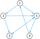
We first evaluated the convergence performance of our proposed Algorithm 1. In this simulation, we considered a network of N=5𝑁5N=5 nodes interacting on a strongly connected graph, which is shown in Fig. 1. ε𝜀\varepsilon was set to 0.010.010.01. For iterations kK𝑘𝐾k\leq K, following the requirements of Algorithm 1, the coupling weights pijs(k)superscriptsubscript𝑝𝑖𝑗𝑠𝑘p_{ij}^{s}(k) for j𝒩iout{i}𝑗superscriptsubscript𝒩𝑖𝑜𝑢𝑡𝑖j\in\mathcal{N}_{i}^{out}\cup\{i\} were chosen from (10, 10)1010(-10,\,10). The initial values xi0superscriptsubscript𝑥𝑖0x_{i}^{0} for i=1,,N𝑖1𝑁i=1,\ldots,N were randomly chosen from (0, 50)050(0,\,50). We used e(k)𝑒𝑘e(k) to measure the error between the estimate πi(k)=si(k)/wi(k)subscript𝜋𝑖𝑘subscript𝑠𝑖𝑘subscript𝑤𝑖𝑘\pi_{i}(k)=s_{i}(k)/w_{i}(k) and the true average value α=j=1Nxj0/N𝛼superscriptsubscript𝑗1𝑁superscriptsubscript𝑥𝑗0𝑁\alpha={\sum_{j=1}^{N}x_{j}^{0}}/{N} at iteration k𝑘k, i.e.,

e(k)=𝝅(k)α𝟏=(i=1N(πi(k)α)2)1/2𝑒𝑘norm𝝅𝑘𝛼1superscriptsuperscriptsubscript𝑖1𝑁superscriptsubscript𝜋𝑖𝑘𝛼212\displaystyle e(k)=\big{\|}\boldsymbol{\pi}(k)-\alpha\mathbf{1}\big{\|}=\big{(}\sum\limits_{i=1}^{N}(\pi_{i}(k)-\alpha)^{2}\big{)}^{1/2} (40)

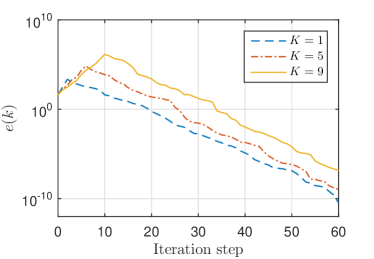
Three experiments were conducted with K𝐾K being set to 111, 555, and 999, respectively. The evolution of e(k)𝑒𝑘e(k) is shown in Fig. 2. It can be seen that e(k)𝑒𝑘e(k) approached to 00, meaning that every node converged to the average value α=j=1Nxj0/N𝛼superscriptsubscript𝑗1𝑁superscriptsubscript𝑥𝑗0𝑁\alpha=\sum_{j=1}^{N}x_{j}^{0}/{N}. It is also worth noting that from Fig. 2, we can see that Algorithm 1 did not start to converge until iteration step kK+1𝑘𝐾1k\geq K+1, which confirmed our analysis in Remark 2.
Refer to caption
Figure 1: Illustration of a strongly connected graph with 555 nodes.
Refer to caption
Figure 2: The evolution of error e(k)𝑒𝑘e(k) under different K𝐾K for a network of 5 nodes.

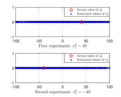
We then evaluated the privacy-preserving performance of Algorithm 1. Under the same network setup as in the previous simulation, we considered the case where a set of honest-but-curious nodes 222, 333, and 444 colluded to infer the initial value x10superscriptsubscript𝑥10x_{1}^{0} of node 111. So we have 𝒜={2, 3, 4}𝒜234\mathcal{A}=\{2,\,3,\,4\}. Note that 𝒩1out𝒩1in={2, 4, 5}𝒜superscriptsubscript𝒩1𝑜𝑢𝑡superscriptsubscript𝒩1𝑖𝑛245not-subset-of𝒜\mathcal{N}_{1}^{out}\cup\mathcal{N}_{1}^{in}=\{2,\,4,\,5\}\not\subset\mathcal{A} holds for node 111. Two experiments were conducted with x10superscriptsubscript𝑥10x_{1}^{0} being set to 404040 and 4040-40, respectively. x20,,x50superscriptsubscript𝑥20superscriptsubscript𝑥50x_{2}^{0},\ldots,x_{5}^{0} were randomly chosen from (0, 50)050(0,\,50). K𝐾K was set to 111. The other parameters were the same as the first simulation, and the maximal iteration step was M=100𝑀100M=100. To infer the value of x10superscriptsubscript𝑥10x_{1}^{0}, the nodes in set 𝒜𝒜\mathcal{A} were able to construct the following linear equations based on the accessible information 𝒜subscript𝒜\mathcal{I_{A}}

s1(k+1)s1(k)+Δs1(k)=p14s(k)s4(k)p21s(k)s1(k)subscript𝑠1𝑘1subscript𝑠1𝑘Δsubscript𝑠1𝑘superscriptsubscript𝑝14𝑠𝑘subscript𝑠4𝑘superscriptsubscript𝑝21𝑠𝑘subscript𝑠1𝑘\displaystyle s_{1}(k+1)-s_{1}(k)+\Delta s_{1}(k)=p_{14}^{s}(k)s_{4}(k)-p_{21}^{s}(k)s_{1}(k) (41)

for k=0,1,,M𝑘01𝑀k=0,1,\ldots,M and

w1(k+1)w1(k)+Δw1(k)=p14w(k)w4(k)p21w(k)w1(k)subscript𝑤1𝑘1subscript𝑤1𝑘Δsubscript𝑤1𝑘superscriptsubscript𝑝14𝑤𝑘subscript𝑤4𝑘superscriptsubscript𝑝21𝑤𝑘subscript𝑤1𝑘\displaystyle w_{1}(k+1)-w_{1}(k)+\Delta w_{1}(k)=p_{14}^{w}(k)w_{4}(k)-p_{21}^{w}(k)w_{1}(k) (42)

for k=K+1,,M𝑘𝐾1𝑀k=K+1,\ldots,M where Δs1(k)Δsubscript𝑠1𝑘\Delta s_{1}(k) and Δw1(k)Δsubscript𝑤1𝑘\Delta w_{1}(k) are given by

Δs1(k)=p51s(k)s1(k)Δsubscript𝑠1𝑘superscriptsubscript𝑝51𝑠𝑘subscript𝑠1𝑘\displaystyle\Delta s_{1}(k)=p_{51}^{s}(k)s_{1}(k)
Δw1(k)=p51w(k)w1(k)Δsubscript𝑤1𝑘superscriptsubscript𝑝51𝑤𝑘subscript𝑤1𝑘\displaystyle\Delta w_{1}(k)=p_{51}^{w}(k)w_{1}(k)

Given p21s(k)=p21w(k)superscriptsubscript𝑝21𝑠𝑘superscriptsubscript𝑝21𝑤𝑘p_{21}^{s}(k)=p_{21}^{w}(k) for kK+1𝑘𝐾1k\geq K+1, set 𝒜𝒜\mathcal{A} also constructed the following relationship

s1(k)π1(k)w1(k)=0subscript𝑠1𝑘subscript𝜋1𝑘subscript𝑤1𝑘0s_{1}(k)-\pi_{1}(k)w_{1}(k)=0 (43)

for k=K+1,K+2,,M𝑘𝐾1𝐾2𝑀k=K+1,K+2,\ldots,M where π1(k)=p21s(k)s1(k)/p21w(k)w1(k)subscript𝜋1𝑘superscriptsubscript𝑝21𝑠𝑘subscript𝑠1𝑘superscriptsubscript𝑝21𝑤𝑘subscript𝑤1𝑘\pi_{1}(k)={p_{21}^{s}(k)s_{1}(k)}/{p_{21}^{w}(k)w_{1}(k)} is known to set 𝒜𝒜\mathcal{A} since both p21s(k)s1(k)superscriptsubscript𝑝21𝑠𝑘subscript𝑠1𝑘{p_{21}^{s}(k)s_{1}(k)} and p21w(k)w1(k)superscriptsubscript𝑝21𝑤𝑘subscript𝑤1𝑘{p_{21}^{w}(k)w_{1}(k)} belong to 𝒜subscript𝒜\mathcal{I_{A}}.

The total number of linear equations (41), (42), and (43) is 3M2K+13𝑀2𝐾13M-2K+1, and in these equations there are 4M2K+34𝑀2𝐾34M-2K+3 variables unknown to set 𝒜𝒜\mathcal{A}, i.e., s1(0),,s1(M+1),Δs1(0),,Δs1(M),w1(K+2),,w1(M+1),Δw1(K+1),subscript𝑠10subscript𝑠1𝑀1Δsubscript𝑠10Δsubscript𝑠1𝑀subscript𝑤1𝐾2subscript𝑤1𝑀1Δsubscript𝑤1𝐾1s_{1}(0),\ldots,s_{1}(M+1),\Delta s_{1}(0),\ldots,\Delta s_{1}(M),w_{1}(K+2),\ldots,w_{1}(M+1),\Delta w_{1}(K+1), ,Δw1(M)Δsubscript𝑤1𝑀\ldots,\Delta w_{1}(M). So there are infinitely many solutions since the number of equations is less than the number of unknown variables. In order to uniquely determine the value of x10superscriptsubscript𝑥10x_{1}^{0}, we used the least-squares solution to estimate x10superscriptsubscript𝑥10x_{1}^{0}. In each experiment, set 𝒜𝒜\mathcal{A} estimated x10superscriptsubscript𝑥10x_{1}^{0} for 100010001000 times, with recorded estimation results shown in Fig. 3. It can be seen that set 𝒜𝒜\mathcal{A} cannot get a good estimate of x10superscriptsubscript𝑥10x_{1}^{0}.

Refer to caption
Figure 3: Estimation of x10superscriptsubscript𝑥10x_{1}^{0} by the set of honest-but-curious nodes 222, 333, and 444. In each experiment, the actual value of x10superscriptsubscript𝑥10x_{1}^{0} is represented by the star, and the estimated values of x10superscriptsubscript𝑥10x_{1}^{0} are represented by the x-marks.

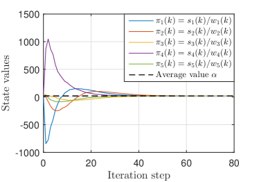
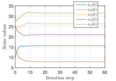
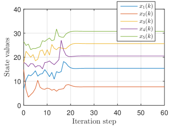
We also compared our Algorithm 1 with existing data-obfuscation based approaches, more specifically, the differential-privacy based approach in [12], the finite-noise-sequence approach in [19], and the decaying-noise approach in [21]. Under the same network setup as in the previous simulations, we set the initial values to {10,15,20,25,30}1015202530\{10,15,20,25,30\}, respectively, with the average value given by 202020. The weight matrix 𝐖𝐖\mathbf{W} was adopted from [12], i.e., the ij𝑖𝑗ij-th entry was set to wij=1/(|𝒩jout|+1)subscript𝑤𝑖𝑗1superscriptsubscript𝒩𝑗𝑜𝑢𝑡1w_{ij}={1}/{(|\mathcal{N}_{j}^{out}|+1)} for i𝒩jout{j}𝑖superscriptsubscript𝒩𝑗𝑜𝑢𝑡𝑗i\in\mathcal{N}_{j}^{out}\cup\{j\} and wij=0subscript𝑤𝑖𝑗0w_{ij}=0 for i𝒩jout{j}𝑖superscriptsubscript𝒩𝑗𝑜𝑢𝑡𝑗i\notin\mathcal{N}_{j}^{out}\cup\{j\}. Since the graph is directed and imbalanced, and does not satisfy the undirected or balanced assumption in [12, 19, 21], the approaches in [12, 19, 21] failed to achieve average consensus, as confirmed by the numerical simulation results in Fig. 4, Fig. 5, and Fig. 6, respectively.
Refer to caption
Figure 4: The evolution of xi(k)subscript𝑥𝑖𝑘x_{i}(k) under the approach proposed in [12].
Refer to caption
Figure 5: The evolution of xi(k)subscript𝑥𝑖𝑘x_{i}(k) under the approach proposed in [19].
Refer to caption
Figure 6: The evolution of xi(k)subscript𝑥𝑖𝑘x_{i}(k) under the approach proposed in [21].

V-B Hardware Experiments

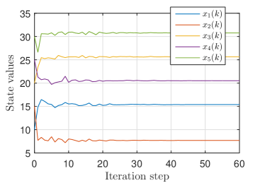
To confirm the efficiency of our proposed Algorithm 2 in real-world embedded systems, we also implemented our algorithm on five Raspberry Pi boards with 64-bit ARMv8 CPU and 1 GB RAM. In the hardware implementation, the communication was conducted through Wi-Fi based on the “sys/socket.h” C library. Paillier encryption/decryption was realized using the “libpaillier-0.8” library from [40]. Since in the implementation, it was impossible to start all nodes simultaneously, a counter was introduced on each node which helped nodes to stay on the same pace. For 256256256-bit encryption key, the size of the actual packet was 136136136 bytes, which included all necessary headers and stuffing bytes. The interaction graph is still Fig. 1. The initial values of the five nodes were set to {10,15,20,25,30}1015202530\{10,15,20,25,30\}, which have an average value of 202020. K𝐾K and ε𝜀\varepsilon were set to 111 and 0.010.010.01, respectively. The coupling weights pijs(k)superscriptsubscript𝑝𝑖𝑗𝑠𝑘p_{ij}^{s}(k) for kK𝑘𝐾k\leq K were chosen from (10, 10)1010(-10,\,10). For each encryption, the average processing latency was 12.15 ms, which is acceptable for most real-time control systems. The implementation result is given in Fig. 7, which shows that for each node i𝑖i, the estimate πisubscript𝜋𝑖\pi_{i} converged to the exact average value α=20𝛼20\alpha=20.

Refer to caption
Figure 7: The evolution of each estimate πi(k)subscript𝜋𝑖𝑘\pi_{i}(k) in the hardware implementation on five Raspberry Pi boards.

VI Conclusions

We proposed a privacy-preserving average consensus approach for directed graphs. Different from existing differential-privacy based approaches which inject noise to exchanged states and thus compromise accuracy, we leverage the inherent robustness of consensus dynamics to embed privacy in random coupling weights, which guarantees consensus to the exact value. Furthermore, the approach can be combined with encryption to protect against eavesdroppers which fail all correlated-noise based privacy-preserving average consensus approaches. Experimental results on embedded micro-controllers confirm that the computational burden is manageable on resource-restricted systems.

Proof of Lemma 1: Given 𝐰(0)=𝟏𝐰01\mathbf{w}(0)=\mathbf{1} and 𝐏w(k)=𝐈subscript𝐏𝑤𝑘𝐈\mathbf{P}_{w}(k)=\mathbf{I} for k=0,1,,K𝑘01𝐾k=0,1,\ldots,K, it is easy to obtain wi(k)=1subscript𝑤𝑖𝑘1w_{i}(k)=1 for kK+1𝑘𝐾1k\leq K+1 from (5).

Since 𝐰(K+1)=𝟏𝐰𝐾11\mathbf{w}(K+1)=\mathbf{1} holds, from (8) we have

𝐰(K+l+1)=𝚽w(K+l:K+1)𝟏\displaystyle\mathbf{w}(K+l+1)=\mathbf{\Phi}_{w}(K+l:K+1)\mathbf{1} (44)

for l1𝑙1l\geq 1. Define δ(l)𝛿𝑙\delta(l) as

δ(l)𝛿𝑙\displaystyle\delta(l) min1iNwi(K+l+1)absentsubscript1𝑖𝑁subscript𝑤𝑖𝐾𝑙1\displaystyle\triangleq\min_{1\leq i\leq N}{w}_{i}(K+l+1) (45)
=min1iN[𝚽w(K+l:K+1) 1]i\displaystyle=\min_{1\leq i\leq N}[\mathbf{\Phi}_{w}(K+l:K+1)\,\mathbf{1}]_{i}

for l1𝑙1l\geq 1. To prove wi(k)εNsubscript𝑤𝑖𝑘superscript𝜀𝑁w_{i}(k)\geq\varepsilon^{N} for kK+2𝑘𝐾2k\geq K+2, i.e., wi(K+l+1)εNsubscript𝑤𝑖𝐾𝑙1superscript𝜀𝑁w_{i}(K+l+1)\geq\varepsilon^{N} for l1𝑙1l\geq 1, it suffices to prove δ(l)εN𝛿𝑙superscript𝜀𝑁\delta(l)\geq\varepsilon^{N} for l1𝑙1l\geq 1. Next, we divide the proof into two parts: 1lN1𝑙𝑁1\leq l\leq N and lN+1𝑙𝑁1l\geq N+1.

Part 1: δ(l)εN𝛿𝑙superscript𝜀𝑁\delta(l)\geq\varepsilon^{N} for 1lN1𝑙𝑁1\leq l\leq N. It is easy to verify that the following relationship exists

[𝚽w(K+l:K+1)]ii=[𝐏w(K+l)𝐏w(K+1)]ii\displaystyle[\mathbf{\Phi}_{w}(K+l:K+1)]_{ii}=[\mathbf{P}_{w}(K+l)\cdots\mathbf{P}_{w}(K+1)]_{ii}
\displaystyle\geq [𝐏w(K+l)]ii[𝐏w(K+l1)𝐏w(K+1)]iisubscriptdelimited-[]subscript𝐏𝑤𝐾𝑙𝑖𝑖subscriptdelimited-[]subscript𝐏𝑤𝐾𝑙1subscript𝐏𝑤𝐾1𝑖𝑖\displaystyle[\mathbf{P}_{w}(K+l)]_{ii}\,[\mathbf{P}_{w}(K+l-1)\cdots\mathbf{P}_{w}(K+1)]_{ii}
\displaystyle\geq ε[𝚽w(K+l1:K+1)]ii\displaystyle\varepsilon\,[\mathbf{\Phi}_{w}(K+l-1:K+1)]_{ii}

Given [𝚽w(K+1:K+1)]ii=[𝐏w(K+1)]iiε[\mathbf{\Phi}_{w}(K+1:K+1)]_{ii}=[\mathbf{P}_{w}(K+1)]_{ii}\geq\varepsilon, we have [𝚽w(K+l:K+1)]iiεl[\mathbf{\Phi}_{w}(K+l:K+1)]_{ii}\geq\varepsilon^{l}. So it follows naturally that

[𝚽w(K+l:K+1) 1]i[𝚽w(K+l:K+1)]iiεlεN[\mathbf{\Phi}_{w}(K+l:K+1)\,\mathbf{1}]_{i}\geq[\mathbf{\Phi}_{w}(K+l:K+1)]_{ii}\geq\varepsilon^{l}\geq\varepsilon^{N}

holds for i=1,,N𝑖1𝑁i=1,\ldots,N and 1lN1𝑙𝑁1\leq l\leq N, meaning that δ(l)εN𝛿𝑙superscript𝜀𝑁\delta(l)\geq\varepsilon^{N} holds for 1lN1𝑙𝑁1\leq l\leq N.

Part 2: δ(l)εN𝛿𝑙superscript𝜀𝑁\delta(l)\geq\varepsilon^{N} for lN+1𝑙𝑁1l\geq N+1. Given lN+1𝑙𝑁1l\geq N+1 and 𝚽w(K+l:K+lN+1)=𝐏w(K+l)𝐏w(K+lN+1)\mathbf{\Phi}_{w}(K+l:K+l-N+1)=\mathbf{P}_{w}(K+l)\cdots\mathbf{P}_{w}(K+l-N+1), we have the following relationship according to (8)

𝐰(K+l+1)=𝚽w(K+l:K+lN+1)𝐰(K+lN+1)\mathbf{w}(K+l+1)=\mathbf{\Phi}_{w}(K+l:K+l-N+1)\,\mathbf{w}(K+l-N+1)

Letting 𝐰(K+lN+1)𝐰𝐾𝑙𝑁1\mathbf{w}(K+l-N+1) be a standard basis vector 𝐞jsubscript𝐞𝑗\mathbf{e}_{j} where the j𝑗j-th entry of 𝐞jsubscript𝐞𝑗\mathbf{e}_{j} is 111 and all other entries are 00, we have

wi(K+l+1)=[𝚽w(K+l:K+lN+1)]ijw_{i}(K+l+1)=[\mathbf{\Phi}_{w}(K+l:K+l-N+1)]_{ij}

Next, we prove

[𝚽w(K+l:K+lN+1)]ijεN[\mathbf{\Phi}_{w}(K+l:K+l-N+1)]_{ij}\geq\varepsilon^{N}

for 1i,jNformulae-sequence1𝑖𝑗𝑁1\leq i,\,j\leq N, which is equivalent to wi(K+l+1)εNsubscript𝑤𝑖𝐾𝑙1superscript𝜀𝑁w_{i}(K+l+1)\geq\varepsilon^{N} under 𝐰(K+lN+1)=𝐞j𝐰𝐾𝑙𝑁1subscript𝐞𝑗\mathbf{w}(K+l-N+1)=\mathbf{e}_{j}.

If i=j𝑖𝑗i=j holds, given 𝐰(k+1)=𝐏w(k)𝐰(k)𝐰𝑘1subscript𝐏𝑤𝑘𝐰𝑘\mathbf{w}(k+1)=\mathbf{P}_{w}(k)\mathbf{w}(k) and [𝐏w(k)]iiεsubscriptdelimited-[]subscript𝐏𝑤𝑘𝑖𝑖𝜀[\mathbf{P}_{w}(k)]_{ii}\geq\varepsilon for kK+1𝑘𝐾1k\geq K+1, we have wi(k+1)εwi(k)subscript𝑤𝑖𝑘1𝜀subscript𝑤𝑖𝑘w_{i}(k+1)\geq\varepsilon\,w_{i}(k). Using the fact wi(K+lN+1)=1subscript𝑤𝑖𝐾𝑙𝑁11w_{i}(K+l-N+1)=1, one can easily verify wi(K+l+1)εNsubscript𝑤𝑖𝐾𝑙1superscript𝜀𝑁w_{i}(K+l+1)\geq\varepsilon^{N}, implying [𝚽w(K+l:K+lN+1)]iiεN[\mathbf{\Phi}_{w}(K+l:K+l-N+1)]_{ii}\geq\varepsilon^{N} for 1iN1𝑖𝑁1\leq i\leq N.

If ij𝑖𝑗i\neq j holds, since the graph 𝒢𝒢\mathcal{G} is strongly connected, there must exist a path from node j𝑗j to node i𝑖i. Denote the path as v1v2vrsubscript𝑣1subscript𝑣2subscript𝑣𝑟v_{1}\shortrightarrow v_{2}\shortrightarrow\cdots\shortrightarrow v_{r} where v1=jsubscript𝑣1𝑗v_{1}=j, vr=isubscript𝑣𝑟𝑖v_{r}=i, and rN𝑟𝑁r\leq N. Since [𝐏w(K+lN+k)]vk+1vkεsubscriptdelimited-[]subscript𝐏𝑤𝐾𝑙𝑁𝑘subscript𝑣𝑘1subscript𝑣𝑘𝜀[\mathbf{P}_{w}(K+l-N+k)]_{v_{k+1}v_{k}}\geq\varepsilon holds for 1kr11𝑘𝑟11\leq k\leq r-1, we have

wvk+1(K+lN+k+1)εwvk(K+lN+k)subscript𝑤subscript𝑣𝑘1𝐾𝑙𝑁𝑘1𝜀subscript𝑤subscript𝑣𝑘𝐾𝑙𝑁𝑘w_{v_{k+1}}(K+l-N+k+1)\geq\varepsilon w_{v_{k}}(K+l-N+k)

Given wv1(K+lN+1)=wj(K+lN+1)=1subscript𝑤subscript𝑣1𝐾𝑙𝑁1subscript𝑤𝑗𝐾𝑙𝑁11w_{v_{1}}(K+l-N+1)=w_{j}(K+l-N+1)=1,

wvr(K+lN+r)=wi(K+lN+r)εr1subscript𝑤subscript𝑣𝑟𝐾𝑙𝑁𝑟subscript𝑤𝑖𝐾𝑙𝑁𝑟superscript𝜀𝑟1w_{v_{r}}(K+l-N+r)=w_{i}(K+l-N+r)\geq\varepsilon^{r-1}

holds. Further taking into account the facts [𝐏w(k)]iiεsubscriptdelimited-[]subscript𝐏𝑤𝑘𝑖𝑖𝜀[\mathbf{P}_{w}(k)]_{ii}\geq\varepsilon for kK+1𝑘𝐾1k\geq K+1, we have

wi(K+l+1)εNr+1wi(K+lN+r)εNr+1εr1=εNsubscript𝑤𝑖𝐾𝑙1superscript𝜀𝑁𝑟1subscript𝑤𝑖𝐾𝑙𝑁𝑟superscript𝜀𝑁𝑟1superscript𝜀𝑟1superscript𝜀𝑁w_{i}(K+l+1)\geq\varepsilon^{N-r+1}w_{i}(K+l-N+r)\geq\varepsilon^{N-r+1}\varepsilon^{r-1}=\varepsilon^{N}

which implies

[𝚽w(K+l:K+lN+1)]ijεN[\mathbf{\Phi}_{w}(K+l:K+l-N+1)]_{ij}\geq\varepsilon^{N}

for 1ijN1𝑖𝑗𝑁1\leq i\neq j\leq N.

Therefore, we have [𝚽w(K+l:K+lN+1)]ijεN[\mathbf{\Phi}_{w}(K+l:K+l-N+1)]_{ij}\geq\varepsilon^{N} for 1i,jNformulae-sequence1𝑖𝑗𝑁1\leq i,\,j\leq N. Since lN+1𝑙𝑁1l\geq N+1 holds and 𝐏w(k)subscript𝐏𝑤𝑘\mathbf{P}_{w}(k) is column stochastic,

𝚽w(K+lN:K+1)=𝐏w(K+lN)𝐏w(K+1)\mathbf{\Phi}_{w}(K+l-N:K+1)=\mathbf{P}_{w}(K+l-N)\cdots\mathbf{P}_{w}(K+1)

is also column stochastic. Further taking into account the fact

𝚽w(K+l:K+1)\displaystyle\mathbf{\Phi}_{w}(K+l:K+1)
=\displaystyle= 𝚽w(K+l:K+lN+1)𝚽w(K+lN:K+1)\displaystyle\mathbf{\Phi}_{w}(K+l:K+l-N+1)\mathbf{\Phi}_{w}(K+l-N:K+1)

leads to

[𝚽w(K+l:K+1)]ijεN[\mathbf{\Phi}_{w}(K+l:K+1)]_{ij}\geq\varepsilon^{N}

for 1i,jNformulae-sequence1𝑖𝑗𝑁1\leq i,\,j\leq N. So it can be easily verified that

[𝚽w(K+l:K+1) 1]iNεNεN[\mathbf{\Phi}_{w}(K+l:K+1)\,\mathbf{1}]_{i}\geq N\varepsilon^{N}\geq\varepsilon^{N}

holds for i=1,,N𝑖1𝑁i=1,\ldots,N, meaning that δ(l)εN𝛿𝑙superscript𝜀𝑁\delta(l)\geq\varepsilon^{N} holds for lN+1𝑙𝑁1l\geq N+1.

Therefore, δ(l)εN𝛿𝑙superscript𝜀𝑁\delta(l)\geq\varepsilon^{N} holds for l1𝑙1l\geq 1, which implies wi(K+l+1)εNsubscript𝑤𝑖𝐾𝑙1superscript𝜀𝑁w_{i}(K+l+1)\geq\varepsilon^{N} for l1𝑙1l\geq 1. In conclusion, we have wi(k)=1subscript𝑤𝑖𝑘1w_{i}(k)=1 for kK+1𝑘𝐾1k\leq K+1 and wi(k)εNsubscript𝑤𝑖𝑘superscript𝜀𝑁w_{i}(k)\geq\varepsilon^{N} for kK+2𝑘𝐾2k\geq K+2. \blacksquare

Acknowledgment

The authors would like to thank Chunlei Zhang and Muaz Ahmad for valuable discussions and help with experimental verification.

References

  • [1] H. Gao, C. Zhang, M. Ahmad, and Y. Q. Wang, “Privacy-preserving average consensus on directed graphs using push-sum,” in 2018 IEEE Conference on Communications and Network Security (CNS).   IEEE, 2018.
  • [2] J. E. Boillat, “Load balancing and poisson equation in a graph,” Concurrency and Computation: Practice and Experience, vol. 2, no. 4, pp. 289–313, 1990.
  • [3] G. Cybenko, “Dynamic load balancing for distributed memory multiprocessors,” J. Parallel Distrib. Comput., vol. 7, no. 2, pp. 279–301, 1989.
  • [4] N. A. Lynch, Distributed algorithms.   San Francisco, CA: Morgan Kaufmann Publishers, 1996.
  • [5] D. S. Scherber and H. C. Papadopoulos, “Locally constructed algorithms for distributed computations in ad-hoc networks,” in Proceedings of the 3rd international symposium on Information processing in sensor networks.   ACM, 2004, pp. 11–19.
  • [6] L. Xiao, S. Boyd, and S. Lall, “A scheme for robust distributed sensor fusion based on average consensus,” in Proceedings of the 4th international symposium on Information processing in sensor networks.   IEEE Press, 2005, p. 9.
  • [7] R. Olfati-Saber and R. M. Murray, “Consensus problems in networks of agents with switching topology and time-delays,” IEEE Trans. Autom. Control, vol. 49, no. 9, pp. 1520–1533, 2004.
  • [8] W. Ren and R. W. Beard, “Consensus seeking in multiagent systems under dynamically changing interaction topologies,” IEEE Trans. Autom. Control, vol. 50, no. 5, pp. 655–661, 2005.
  • [9] R. Hoenkamp, G. B. Huitema, and A. J. C. de Moor-van Vugt, “The neglected consumer: the case of the smart meter rollout in the netherlands,” Renew. Energy Law Policy Rev., pp. 269–282, 2011.
  • [10] J. N. Tsitsiklis, “Problems in decentralized decision making and computation,” Ph.D. dissertation, 1984.
  • [11] Z. Zhang and M. Y. Chow, “Incremental cost consensus algorithm in a smart grid environment,” in 2011 IEEE Power and Energy Society General Meeting, 2011, pp. 1–6.
  • [12] Z. Huang, S. Mitra, and G. Dullerud, “Differentially private iterative synchronous consensus,” in Proceedings of the 2012 ACM workshop on Privacy in the electronic society, 2012, pp. 81–90.
  • [13] E. Nozari, P. Tallapragada, and J. Cortés, “Differentially private average consensus with optimal noise selection,” IFAC-PapersOnLine, vol. 48, no. 22, pp. 203–208, 2015.
  • [14] Z. Huang, S. Mitra, and N. Vaidya, “Differentially private distributed optimization,” in Proceedings of the 2015 International Conference on Distributed Computing and Networking, 2015, pp. 4:1–4:10.
  • [15] E. Nozari, P. Tallapragada, and J. Cortés, “Differentially private average consensus: obstructions, trade-offs, and optimal algorithm design,” Automatica, vol. 81, pp. 221–231, 2017.
  • [16] V. Katewa, F. Pasqualetti, and V. Gupta, “On privacy vs cooperation in multi-agent systems,” Int. J. Control, no. accepted, pp. 1–20, 2017.
  • [17] Y. Wang, Z. Huang, S. Mitra, and G. E. Dullerud, “Differential privacy in linear distributed control systems: Entropy minimizing mechanisms and performance tradeoffs,” IEEE Trans. Control Netw. Syst., vol. 4, no. 1, pp. 118–130, 2017.
  • [18] M. Kefayati, M. S. Talebi, B. H. Khalaj, and H. R. Rabiee, “Secure consensus averaging in sensor networks using random offsets,” in IEEE International Conference on Telecommunications and Malaysia International Conference on Communications, 2007, pp. 556–560.
  • [19] N. E. Manitara and C. N. Hadjicostis, “Privacy-preserving asymptotic average consensus,” in 2013 European Control Conference (ECC), 2013, pp. 760–765.
  • [20] J. He, L. Cai, P. Cheng, M. Xing, J. Pan, and L. Shi, “Private and accurate data aggregation against dishonest nodes,” arXiv preprint arXiv:1609.06381, 2016.
  • [21] Y. Mo and R. M. Murray, “Privacy preserving average consensus,” IEEE Trans. Autom. Control, vol. 62, no. 2, pp. 753–765, 2017.
  • [22] S. Pequito, S. Kar, S. Sundaram, and A. P. Aguiar, “Design of communication networks for distributed computation with privacy guarantees,” in In Decision and Control (CDC), 2014 IEEE 53rd Annual Conference on, 2014, pp. 1370–1376.
  • [23] A. Alaeddini, K. Morgansen, and M. Mesbah, “Adaptive communication networks with privacy guarantees,” in Proceedings of 2017 American Control Conference, 2017, pp. 4460–4465.
  • [24] M. Ruan, M. Ahmad, and Y. Q. Wang, “Secure and privacy-preserving average consensus,” in The 3rd ACM Workshop on Cyber-Physical Systems Security & Privacy, accepted.
  • [25] A. D. Domínguez-García and C. N. Hadjicostis, “Distributed strategies for average consensus in directed graphs,” in 2011 50th IEEE Conference on Decision and Control and European Control Conference (CDC-ECC), 2011, pp. 2124–2129.
  • [26] B. Gharesifard and J. Cortés, “Distributed strategies for generating weight-balanced and doubly stochastic digraphs,” European Journal of Control, vol. 18, no. 6, pp. 539–557, 2012.
  • [27] D. Kempe, A. Dobra, and J. Gehrke, “Gossip-based computation of aggregate information,” in Proceedings of 44th Annual IEEE Symposium on Foundations of Computer Science, 2003, pp. 482–491.
  • [28] F. Bénézit, V. Blondel, P. Thiran, J. Tsitsiklis, and M. Vetterli, “Weighted gossip: Distributed averaging using non-doubly stochastic matrices,” in Proceedings of 2010 IEEE International Symposium on Information Theory, 2010, pp. 1753–1757.
  • [29] E. Seneta, Non-negative Matrices and Markov Chains.   Springer, 1973.
  • [30] J. A. Fill, “Eigenvalue bounds on convergence to stationarity for nonreversible markov chains, with an application to the exclusion process,” The annals of applied probability, pp. 62–87, 1991.
  • [31] P. Paillier, “Public-key cryptosystems based on composite degree residuosity classes,” in Eurocrypt, vol. 99.   Springer Berlin Heidelberg, 1999, pp. 223–238.
  • [32] K. Liu, H. Kargupta, and J. Ryan, “Random projection-based multiplicative data perturbation for privacy preserving distributed data mining,” IEEE Trans. Knowl. Data Eng., vol. 18, no. 1, pp. 92–106, 2006.
  • [33] S. Han, W. K. Ng, L. Wan, and V. C. S. Lee, “Privacy-preserving gradient-descent methods,” IEEE Trans. Knowl. Data Eng., vol. 22, no. 6, pp. 884–899, 2010.
  • [34] N. Cao, C. Wang, M. Li, K. Ren, and W. Lou, “Privacy-preserving multi-keyword ranked search over encrypted cloud data,” IEEE Trans. Parallel Distrib. Syst., vol. 25, no. 1, pp. 222–233, 2014.
  • [35] A. Nedić, A. Olshevsky, and W. Shi, “Achieving geometric convergence for distributed optimization over time-varying graphs,” SIAM Journal on Optimization, vol. 27, no. 4, pp. 2597–2633, 2017.
  • [36] ——, “A geometrically convergent method for distributed optimization over time-varying graphs,” in Decision and Control (CDC), 2016 IEEE 55th Conference on.   IEEE, 2016, pp. 1023–1029.
  • [37] A. Nedić, A. Ozdaglar, and P. A. Parrilo, “Constrained consensus and optimization in multi-agent networks,” IEEE Transactions on Automatic Control, vol. 55, no. 4, pp. 922–938, 2010.
  • [38] A. S. Tanenbaum and D. Wetherall, Computer networks.   Pearson Prentice Hall, 2011.
  • [39] O. Goldreich, Foundations of cryptography: volume 2, basic applications.   Cambridge university press, 2009.
  • [40] Paillier Library, http://acsc.cs.utexas.edu/libpaillier/.
Huan Gao (S’16) was born in Shandong, China. He received the B.S. and M.Sc. degrees in automation and control theory and control engineering from Northwestern Polytechnical University, Shaanxi, China, in 2011 and 2015, respectively. He is currently working toward the Ph.D. degree in the Department of Electrical and Computer Engineering, Clemson University, Clemson, SC, USA. His current research focuses on dynamics of pulse-coupled oscillators and cooperative control of multi-agent systems.
Yongqiang Wang (SM’13) was born in Shandong, China. He received the B.S. degree in Electrical Engineering & Automation, the B.S. degree in Computer Science & Technology from Xi’an Jiaotong University, Shaanxi, China, in 2004. He received the M.Sc. and the Ph.D. degrees in Control Science & Engineering from Tsinghua University, Beijing, China, in 2009. From 2007-2008, he was with the University of Duisburg-Essen, Germany, as a visiting student. He was a Project Scientist at the University of California, Santa Barbara. He is currently an Assistant Professor with the Department of Electrical and Computer Engineering, Clemson University, Clemson, SC, USA. His research interests are cooperative and networked control, synchronization of wireless sensor networks, systems modeling and analysis of biochemical oscillator networks, and model-based fault diagnosis. He received the 2008 Young Author Prize from IFAC Japan Foundation for a paper presented at the 17th IFAC World Congress in Seoul.