Comparative Document Summarisation via Classification
Abstract
This paper considers extractive summarisation in a comparative setting: given two or more document groups (e.g., separated by publication time), the goal is to select a small number of documents that are representative of each group, and also maximally distinguishable from other groups. We formulate a set of new objective functions for this problem that connect recent literature on document summarisation, interpretable machine learning, and data subset selection. In particular, by casting the problem as a binary classification amongst different groups, we derive objectives based on the notion of maximum mean discrepancy, as well as a simple yet effective gradient-based optimisation strategy. Our new formulation allows scalable evaluations of comparative summarisation as a classification task, both automatically and via crowd-sourcing. To this end, we evaluate comparative summarisation methods on a newly curated collection of controversial news topics over 13 months. We observe that gradient-based optimisation outperforms discrete and baseline approaches in 14 out of 24 different automatic evaluation settings. In crowd-sourced evaluations, summaries from gradient optimisation elicit 7% more accurate classification from human workers than discrete optimisation. Our result contrasts with recent literature on submodular data subset selection that favours discrete optimisation. We posit that our formulation of comparative summarisation will prove useful in a diverse range of use cases such as comparing content sources, authors, related topics, or distinct view points.
1 Introduction
Extractive summarisation is the task of selecting a few representative documents from a larger collection. In this paper, we consider comparative summarisation: given groups of document collections, the aim is to select documents that represent each group, but also highlight differences between groups. This is in contrast to traditional document summaries which aim to represent each group by independently optimising for coverage and diversity, without considering other groups. As a concrete example, given thousands of news articles per month on a certain topic, groups can be formed by publication time, by source, or by political leaning. Comparative summarisation systems can then help answer user questions such as: what is new on the topic of climate change this week, what is different between the coverage in NYTimes and BBC, or what are the key articles covering the carbon tax and the Paris agreement? In this work, we focus on highlighting changes within a long running news topic over time; see Figure 1 for an illustration.
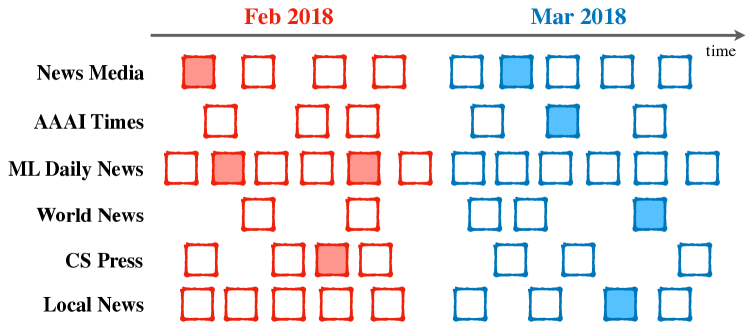
Existing methods for extractive summarisation use a variety of formulations such as structured prediction (?), optimisation of submodular functions (?), dataset interpretability (?), and dataset selection via submodular optimisation (?; ?; ?). Moreover, recent formulations of comparative summarisation use discriminative sentence selection (?; ?), or highlight differences in common concepts across documents (?). But the connections and distinctions of these approaches has yet to be clearly articulated. To evaluate summaries, traditional approaches employ automatic metrics such as ROUGE (?) on manually constructed summaries (?; ?). This is difficult to employ for new tasks and new datasets, and does not scale.
Our approach to comparative summarisation is based on a novel formulation of the problem in terms of two competing classification tasks. Specifically, we formulate the problem as finding summaries for each group such that a powerful classifier can distinguish them from documents belonging to other groups, but cannot distinguish them from documents belonging to the same group. We show how this framework encompasses an existing nearest neighbour objective for summarisation, and propose two new objectives based on the maximum mean discrepancy (?) – mmd-diff which emphasises classification accuracy and mmd-div which emphasises summary diversity – as well as new gradient-based optimisation strategies for these objectives.
A key advantage of our discriminative problem setting is that it allows summarisation to be evaluated as a classification task. To this end, we design automatic and crowd-sourced evaluations for comparative summaries, which we apply on a new dataset of three ongoing controversial news topics. We observe that the new objectives with gradient optimisation are top-performing in 14 out of 24 settings (across news topics, summary size, and classifiers) (§6.2). We design a new crowd-sourced article classification task for human evaluation. We find that workers are on average 7% more accurate in classifying articles using summaries generated by mmd-diff with gradient-based optimisation than all alternatives. Interestingly, our results contrast with the body of work on dataset selection and summarisation that favour discrete greedy optimisation of submodular objectives due to approximation guarantees. We hypothesise that the comparative summarisation problem is particularly amenable to gradient-based optimisation due to the small number of prototypes needed. Moreover, gradient-based approaches can further improve solutions found by greedy approaches.
In sum, the main contributions of this work are:
-
•
A new formulation of comparative document summarisation in terms of competing binary classifiers, two new objectives based on this formulation, and their corresponding gradient-based optimisation strategies.
-
•
Design of a scalable automatic and human evaluation methodology for comparative summarisation models, with results showing that the new objectives out-perform existing submodular objectives.
-
•
A use case of comparatively summarising articles over time from a news topic on a new dataset111Code, datasets and a supplementary appendix are available at https://github.com/computationalmedia/compsumm of three controversial news topics from 2017 to 2018.
2 Related Works
The broader context of this work is extractive summarisation. Approaches to this problem include incorporating diversity measures from information-retrieval (?), structured SVM regularised by constraints for diversity, coverage, and balance (?), or topic models for summarisation (?). Time-aware summarisation is an emerging subproblem, where the current focus is on modeling continuity (?) or continuously updating summaries (?), rather than formulating comparisons. (?; ?) present methods to extract one or few discriminative sentences from a small multi-document corpus utilising greedy optimisation and evaluating qualitatively. (?) compares descriptions about similar concepts in closely related document pairs, leveraging an integer linear program and evaluating with few manually created ground truth summaries. While these works exist in the domain of comparative summarisation, they are either specific to a data domain or have evaluations which are hard to scale up. In this paper we present approaches to comparative summarisation with intuition from competing binary classifiers, leading to different objectives and evaluation. We demonstrate and evaluate the application of these approaches to multiple data domains such as images and text.
Submodular functions have been the preferred form of discrete objectives for summarising text (?), images (?) and data subset selection (?; ?), since they can be optimised greedily with tightly-bounded guarantees. The topic of interpreting dataset and models use similar strategies (?; ?). This work re-investigates classic continuous optimisation for comparative summarisation, and puts it back on the map as a competitive strategy.
3 Comparative Summarisation as Classification
Formally, the comparative summarisation problem is defined on groups of document collections , where a group may, for example, correspond to news articles about a specific topic published in a certain month. We write the document collection for group as
where is the total number of documents in group . We represent individual documents as vector (see §6).
Our goal is to summarise each document collection with a set of summary documents or prototypes , written
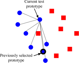
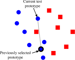
For simplicity, we assume the number of prototypes is the same for each group. The selected prototypes should represent the documents in the group achieving coverage (Figure 2a) and diversity (Figure 2c), while simultaneously discriminating documents from other groups (Figure 2b). For example, if we have news articles on the Climate Change topic then they may discuss the paris agreement in February, coral bleaching in March, and rising sea levels in both months. A comparative summary should include documents about the paris agreement in February and coral bleaching in March, but potentially not on rising sea levels as they are common to both time ranges and hence do not discriminate.

3.1 A Binary Classification Perspective
We now cast comparative summarisation as a binary classification problem. To do so, let us re-interpret the two defining characteristics of prototypes for the th group:
-
(i)
they must represent the documents belonging to that group. Intuitively, this means that each must be indistinguishable from all .
-
(ii)
they must discriminate against documents from all other groups. Intuitively, this means that each must be distinguishable from , where denotes the set of all documents belonging to all groups except .
This lets us relate prototype selection to the familiar binary classification problem: for a good set of prototypes,
-
(a)
there cannot exist a classifier that can accurately discriminate between them and documents from that group. For example, even a powerful classifier should not be able to discriminate prototype documents about the Great Barrier Reef from other documents about the Great Barrier Reef.
-
(b)
there must exist a classifier that can accurately discriminate them against documents from all other groups. For example, a reasonable classifier should be able to discriminate prototypes about the Great Barrier Reef from documents about emission targets.
Consequently, we can think of prototype selection in terms of two competing binary classification objectives: one distinguishing from , and another distinguishing from . In abstract, this suggests a multi-objective optimisation problem of the form
| (1) |
where estimates the accuracy of the best possible classifier for distinguishing between the datasets and . Making this idea practical requires committing to a particular means of balancing the two competing objectives. More interestingly, one also needs to find a tractable way to estimate : explicitly searching over rich classifiers such as deep neural networks, would lead to a computationally challenging nested optimisation problem.
In the following we discuss a set of objective functions that avoid such nested optimisation. We also discuss two simple optimisation strategies for these objectives in §4.
3.2 Prototype Selection via Nearest-neighbour
One existing prototype selection method involves approximating the intragroup term in Eq 1 using nearest-neighbour classifiers, while ignoring the intergroup accuracy term. Specifically, a formulation of prototype selection in (?) maximises the total similarity of every point to its nearest prototype from the same class:
| (2) |
Here, is any similarity function, with admissible choices including a negative distance, or valid kernel functions.
The nearest neighbour utility function is simple and intuitive. However, it only considers the most similar prototype for each datapoint which misses our second desirable property of prototypes: that they explicitly distinguish between different classes. Moreover, the nearest neighbour utility function can be challenging to optimise because of the function. The rest of this section introduces three other utilities that address these concerns.
3.3 Preliminaries: Maximum Mean Discrepancy
The maximum mean discrepancy (MMD) (?) measures the distance between two distributions by leveraging the kernel trick (?). Intuitively, MMD deems two distributions to be close if the mean of every function in some rich class is close under both distributions. For suitable , this is equivalent to comparing the moments of the two distributions; however, a naïve implementation of this idea would require a prohibitive number of evaluations. Fortunately, choosing to be a reproducing kernel Hilbert space (RKHS) with kernel function leads to an expression that is defined only in terms of document interactions via the kernel function (?):
| (3) |
where are observations from two datasets . In practice, it is common to use the radial basis function (RBF) or Gaussian kernel with fixed bandwidth .
One often approximates MMD using sample expectations: given samples from , and samples from , we may compute
| (4) |
3.4 Prototype Selection via MMD
One can think of MMD as implicitly computing a (kernelised) nearest centroid classifier to distinguish between and : MMD is small when this classifier has high expected error. Thus, MMD can be seen as an efficient approximation to classification accuracy . This intuition lead to a practical utility function that approximates Equation 1 by taking the difference of two MMD terms:
|
|
(5) |
The hyper-parameter trades off how well the prototype represents its group, against how well it distinguishes between groups (Figure 2b). Intuitively, when the term is large then the prototypes are dissimilar from documents of other groups. Similarly, when is small then the prototypes are similar to documents of that group. Maximising gives prototypes that are both close to the empirical samples (as seen by the term in Equation 3 and illustrated by Figure 2a) and far from one another (as seen by the term and illustrated by Figure 2c).
While the objective of Equation 5 provides the core of our approach, we also present a variant that increases the diversity of prototypes chosen for each group. A closer examination of the difference of in Equation 5 – by expanding both using Equation 3 – reveals two separate prototype diversity terms and . The latter counteracts the former and decreases prototype diversity (details in Appendix1). On the expanded form of , we remove the terms not involving , as they are constants and have no effect on the solution, and also remove the conflicting diversity term . This gives a new objective:
|
|
(6) |
Maximising encourages prototypes in group to be far from data points in other groups.
One can envision another variant that explicitly optimises the diversity between prototypes of different classes, rather than between prototypes of class against data points in other classes. This is computationally more efficient, and reflects similar intuitions. However, it did not outperform , in summarisation tasks, and is omitted due to space limitations.
Differences to related objectives. The nearest-neighbour objective was articulated in (?) and earlier in (?), and used for classification tasks. Recently, (?) proposed MMD-critic, which selects prototypes for a single group of documents by maximizing The first term in Equation 5 builds on this formulation, applying this idea independently for each group. Our second term is crucial to encourage prototypes that only represent their own group and none of the other groups. MMD-critic also contains model criticisms, which have to be optimized sequentially after obtaining prototypes. As shown in §6, MMD-critic under-performs in comparison tasks by a significant margin.
4 Optimising Utility Functions
There are two general strategies for optimising the utility functions outlined in §3 to generate summaries that are a subset of the original dataset: greedy and gradient optimisation.
Greedy optimisation. The first strategy involves directly choosing prototypes for each group. Obtaining the exact solution to this discrete optimisation problem is intractable; however, approximations such as greedy selection can work well in practice, and may also have theoretical guarantees.
Specifically, suppose we wish to maximise a utility set function defined on ground set . For and , the marginal gain of adding element to an existing set is known as the discrete derivative, and is defined by . We say is monotone if and only if the discrete derivatives are non-negative, i.e. , and is submodular if and only if the marginal gain satisfies diminishing returns, i.e. for , . (?) showed that if is submodular and monotone, greedy maximisation of yields an approximate solution no worse than of the optimal solution under cardinality and matroid constraints. (?) showed this approximation holds with high probability even for non-monotone submodular objectives.
In our context, given a utility function , the greedy algorithm (see Appendix1) works by iteratively picking the that provides the largest marginal gain () one at a time for each group. Among the utility functions mentioned in §3, the nearest-neighbour objective is submodular-monotone (?). The MMD function in Equation 3 is submodular-monotone under mild assumptions on the kernel matrix (?). The MMD objective is the difference between two submodular-monotone functions, which is not submodular in general. On the other hand, the second term in is modular with respect to , when the number of prototypes fixed and known in advance. Therefore, the diversity objective is the difference between a submodular function and a modular function, and thus submodular.
Gradient optimisation The second strategy is to re-cast the problem to allow for continuous optimisation in the feature space, e.g. using standard gradient descent. To generate prototypes, the solutions to this optimisation can then be snapped to the nearest data points as a post-processing step.
Concretely, rather than searching for optimal prototypes directly, we seek “meta-prototypes” , drawn from the same space as the document embeddings. We now modify (Equation 5) to incorporate “meta-prototypes”. Note that can be similarly modified, but cannot, since the function is not differentiable. The “meta-prototypes” for are chosen to optimise
| (7) |
The only difference to Equation 5 is that we do not enforce that . This subtle, but significant, difference allows Equation 7 to be optimized using gradient-following methods. We use L-BFGS (?) with analytical gradients found in online appendix1. The selected meta-prototypes are then snapped to the nearest document in the group: to construct the th prototype for the th group, we find
| (8) |
On a problem often tackled with discrete greedy optimisation, one may wonder if gradient-based methods can be competitive; we answer this in the affirmative in our experiments.
5 Datasets on Controversial News Topics
Exploring the evolution of controversial news topics is a natural application of comparative summarisation. Comparative summarisation could help to better understand the role of news media in such a setting. Recent work on controversial topics (?) focused on the social network and interaction around controversial topics, but did not explicitly consider the content of news articles on these topics. To this end, we curate a set of news articles on long-running controversial topics using tweets which link to news articles. We choose several long-running controversial topics with significant news coverage in 2017 and 2018. To find articles relevant to these topics we use keywords to filter the Twitter stream, and adopt a snowball strategy to add additional keywords (?). The articles linked in these tweets are then de-duplicated and filtered for spam. Article timestamps correspond to the creation time of the first tweet linking to it. Full details of the data collection procedure are described in online appendix1.
In this work, we use news articles on three topics that appeared in a 14 month period (June 2017 – July 2018). Within each topic we comparatively summarise news articles in different time periods to identify what has changed in that topic between the summarisation periods. To ensure our method works on a range of topics we chose substantially different long running topics: Beef Ban – controversy over the slaughter and sale of beef on religious grounds (1543 articles) is localised to a particular region, mainly Indian subcontinent, while Gun Control – restrictions on carrying, using, or purchasing firearms (6494 articles) and Capital Punishment – use of the death penalty (7905 articles) are topical in various regions around the world. Figure 3 shows the number of new articles on each topic over time.
6 Experiments and Results
We evaluate approaches to comparative summarisation using both automatic and crowd-sourced human classification tasks. This choice stems from with our classification perspective (see §3.1), and has been used in the prototype selection literature (?; ?). Intuitively, a good set of prototype articles should uniquely identify a new article’s group.
Datasets and features. We empirically validate classification and prototype selection methods on a well known USPS dataset (?; ?). USPS contains grayscale handwritten digits in 10 classes (i.e., digits 0 through 9). To reduce the dimensionality we use PCA, projecting the 256 dimensional image vectors into 39 features that explain 85% of the variance. The USPS dataset provides 7291 training and 2007 test images. We generate another 9 random splits with exactly the same number of training and test images for the purposes of estimating confidence intervals.
In using the USPS dataset our aims are twofold. First, it shows the versatility of the method: the domain need not be text, collections need not be separated by time, and it operates with more than two classes. Indeed, by thinking of each digit as a group, our method can identify representative and diverse examples of digits. Second, our method can be seen as a special kind of prototype selection for which the USPS dataset has been used as a standard benchmark (?; ?).
We further use the controversial news dataset described in §5 to evaluate comparative summarisation. We adopt the pre-trained GloVe-300 (?) vector representation for each word, and then represent the article as an average of the word vectors from its the title and first 3 sentences – the most important text due to the inverted pyramid structure in news style (?). This feature performs competitively in retrieval tasks despite its simplicity (?). For each news topic, we generate 10 random splits with 80% training articles and 20% test articles for automatic evaluation. One of these splits is used for human evaluation.
Approaches and baselines. We compare:
-
•
nn-comp-greedy represents the nearest neighbour objective , optimised in a greedy manner.
-
•
mmd-diff represents the difference of MMD objective . mmd-diff-grad uses gradient based optimisation while mmd-diff-greedy is optimised greedily.
-
•
mmd-div-grad and mmd-div-greedy are the gradient-based and greedy variants of the diverse MMD objective .
with three baseline approaches:
-
•
kmeans clusters with kmeans++ initialisation (?) found separately for each document group. The cluster centers for each group are snapped to the nearest data point using Equation 8.
-
•
kmedoids (?) clustering algorithm with kmeans++ initialisation, computed separately for each document group. The medoids become the prototypes themselves.
-
•
mmd-critic (?) selects prototypes using greedy optimisation of and criticisms by choosing points that deviate from the prototypes. The summary is selected from the unlabeled training set and consists of prototypes and criticisms in a one-to-one ratio.
We use the Radial Basis Function (RBF) kernel when applicable. The hyper-parameter is chosen along with the trade-off factor , and SVM soft margin using grid search 3 fold cross-validation on the training set. Note that 1NN has no tunable parameters. The grad optimisation approach uses the L-BFGS algorithm (?), with initial prototype guesses chosen by the greedy algorithm for news dataset and K-means for USPS dataset.
6.1 Automatic Evaluation Settings
The controversial news dataset topics are divided into two groups of equal duration based on article timestamp. Note that typically the number of documents in each time range is imbalanced. The USPS hand written digits dataset is divided into 10 groups corresponding to the 10 different digits. On each training split we select the prototypes for each group and then train an SVM or 1NN on the set of prototypes.
We measure the classifier performance on the test set using balanced accuracy, defined as the average accuracy of all classes (?). For binary classification this is , defined in terms of total positives , total negatives , true negatives , and true positives . Balanced accuracy accounts for class imbalance, and is applicable to both binary and multi-class classification tasks (whereas AUC and average precision are not). For all approaches, we report the mean and 95% confidence interval of the 10 random splits.
We report results on 2, 4, 8, or 16 prototypes per group – a small number of prototypes is necessary for the summaries to be meaningful to humans. This is in contrast to the hundreds of prototypes used by (?; ?), in automatic evaluations of the predictive quality of prototypes.
6.2 Automatic Evaluation Results
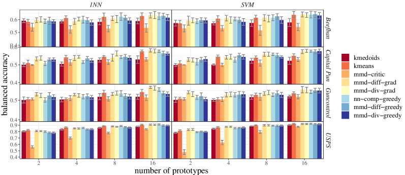
Figure 4 reports balanced accuracy for all methods using SVM and 1-NN across different datasets and numbers of prototypes. On the USPS dataset, most methods perform well. The differences are small, if at all distinguishable. mmd-critic performs poorly on USPS; this is because it does not guarantee a fixed number of prototypes per group, and sometimes misses a group all together. Note that this is very unlikely to occur with only 2 groups in the news dataset.
On the three news datasets, comparative summaries based on mmd objectives are the best-performing approach in 20 out of 24 evaluations (2 classifiers x 4 prototype sizes x 3 news topics (details in Appendix1) . In the remaining two cases, they are the second-best with overlapping confidence intervals against the best (kmeans). Despite the lack of optimisation guarantees, grad optimisation produces prototypes of better quality in 14 out of 24 settings.
Generally, all methods produce better classification accuracy as the number of prototypes increases. This indicates that the chosen prototypes do introduce new information that helps with the classification. In the limit, where all documents are selected as prototypes – a setting that is clearly unreasonable when summarisation is the goal – the performance is determined by the classifier alone. SVM achieves 0.763 on Capital Punishment and Beef Ban, 0.707 on Gun Control, while 1-NN achieves 0.762 on Capital Punishment, 0.763 on Beef Ban and 0.702 on Gun Control. As seen in Figure 4 no prototype selection method approaches this accuracy. This highlights the difficulty of selecting only a few prototypes to represent complex distributions of news articles over time.
6.3 Crowd-sourced Evaluation Settings
We conduct a user study on the crowd-sourcing platform figure-eight222https://www.figure-eight.com with two questions in mind: (1) using article classification accuracy as a proxy, do people perform similarly to automatic evaluation? (2) how useful do people find the comparative summaries? This is an acid test on providing value to users who need comprehend large document corpora. Human evaluations in this work are designed to grade our method in a real world task: accurately identifying a news articles group (e.g. the month it is published) given only a few (4) articles from each month. The automatic evaluations in §6.2 are instructive proxies for efficacy, but inherently incomplete without human evaluation.
Generating summaries for the crowd. We present summaries from four methods kmeans, nn-comp-greedy, mmd-diff-greedy, and mmd-diff-grad – chosen because they perform well in automatic evaluation and together form a cross-section of different method types. We opt to vary the groups of news articles being summarised by choosing many pairs of time ranges, since summaries on the same pair of groups (by definition) tend to be very similar or identical, which incurs user fatigue. We use the Beef Ban topic because it has the longest time range: June 2017 to July 2018 inclusive. The articles are grouped into each of the 14 months, and then 91 (i.e., 14 choose 2) pairs are formed. We take the top 10 pairs by performance according automatic evaluation using each of the four approaches, the union of these lead to 21 pairs. We pick top-performing pairs because preliminary human experiments showed that humans seem unable to classify an article when automatic results do poorly (e.g. 0.65 in balanced accuracy). Articles from each of the 21 pairs of months are randomly split into training and testing sets. We ask participants to classify six randomly sampled test articles. To reduce evaluation variance, all methods share the same test articles, different methods are randomized and are blind to workers. We record three independent judgments for each (test article, month-pair) tuple – totaling 1,512 judgments from 126 test questions over four methods. We also restrict the crowd workers to be from India, where Beef Ban is locally relevant, and workers will be familiar with the people, places and organisations mentioned news articles.
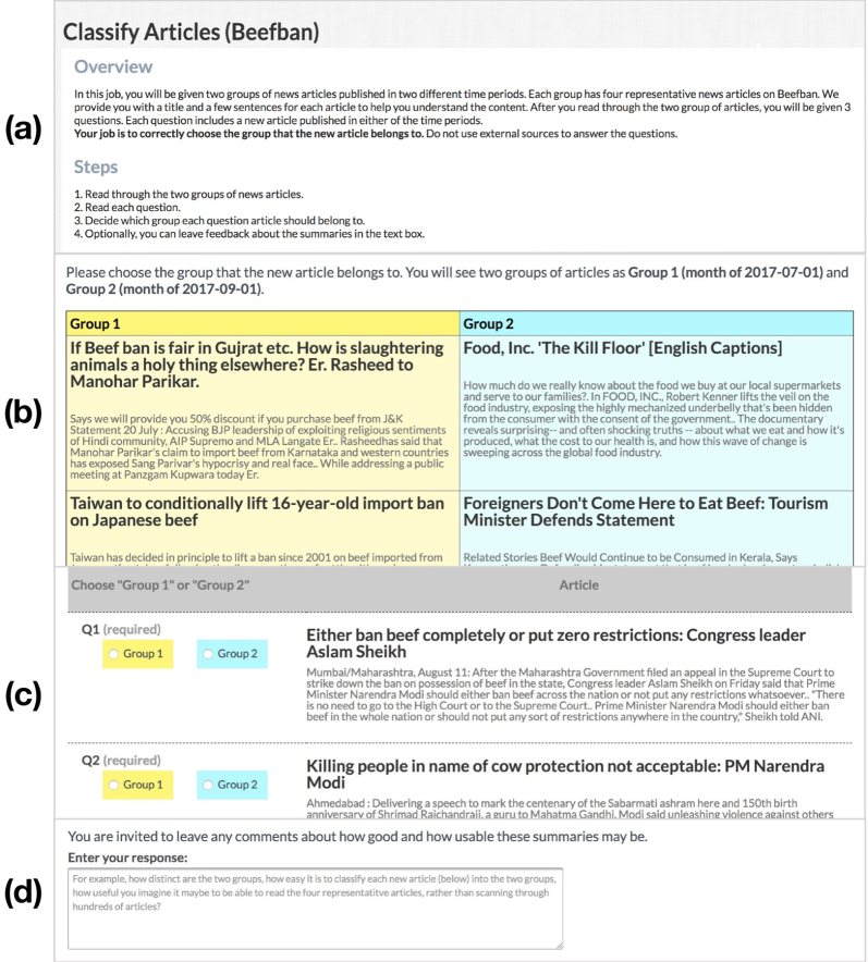
Questionnaire design. Figure 5 shows the questionnaires we designed for human evaluation. Each questionnaire has 4 parts: (a) instructions, (b) two groups of prototypes, (c) test articles that must be classified into a group, and (c) a comment box for free-form feedback.
In the instruction (a), we explain that the two groups of representative articles (the prototypes for each time range) are articles from different time ranges and lay out the steps to complete the questionnaire. We ask participants not to use external sources to help classify test articles.
The two groups of prototype articles (b) are chosen by one of the method being evaluated (e.g., mmd-diff-grad or kmeans) from articles in two different time ranges. Each group has four representative articles and each article has a title and a couple of sentences to help understand the content. We assign a different background colour to each group of summaries to give participants a visual guide.
Below the groups of summary articles are three questions (c), though for brevity only two are shown in Figure 5. Each question asks participants to decide which of the two time ranges a test article belongs to.
We add a comment box (d) to gather free-form feedback from participants. This helps to quickly uncover problems with the task, provides valuable insight into how participants use the summaries to make their choices, and gives an indication of how difficult users find the task. As a quality-control measure, we include questions with known ground truth amongst the test questions. These ground truth questions are manually curated and reviewed if many workers fail on them. Each unit of work includes 4 questionnaires (of 3 questions each), one of which is a group of ground truth questions randomly positioned. Note that ground truth questions are only used to filter out participants and are not included in the evaluation results.
6.4 Crowd-sourced Evaluation Results
Worker profile. The number of unique participants answering test questions ranged from 25 to 31 for each method, indicating that the results were not dominated a small number of participants. On average, participants spent 51 seconds on each test question and 2 minutes 33 seconds on each summary.
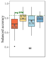
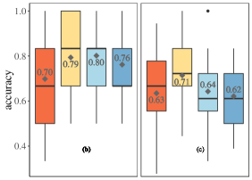

Quantitative results Figure 6 shows that on average crowd workers with mmd-diff-grad summaries classify an article more accurately than summaries from other approaches by at least 7%. The results are statistically significant with under a one sided sign test; which applies because the 126 test questions where answered by three random people and we cannot assume normality. It also has the highest number of consensus correct judgments (details in Appendix1). mmd-diff-greedy performs worse than mmd-diff-grad.
We also compute the Fleiss Kappa statistic to measure inter-annotator agreement. The statistics are: 0.418 for kmeans, 0.456 for mmd-diff-grad, 0.435 for nn-comp-greedy, and 0.483 for mmd-diff-greedy and a combined statistic of 0.451. All statistics fall into the range of moderate agreement (?), which means the results we obtain in crowdsourced evaluations are reliable.
The good performance of gradient-based optimisation is surprising given greedy approaches are usually preferred in subset selection tasks, due to approximation guarantees for submodular objectives. One plausible explanation is that early prototypes selected by greedy tend to cluster around the first prototype, whereas the simultaneous optimisation in grad tend to spread prototypes in feature space. With only four prototypes being shown to users, diversity is an important factor for human classification. Previous studies of greedy methods for prototype selection have used hundreds of prototypes (?) – a setting in which the diversity of the early prototypes matters less – or used criticisms (?) to improve diversity in tandem.
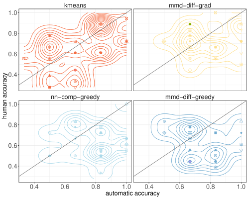
Comparing Figure 6 (a) – (c), automatic classifiers trained on both the entire training set and prototypes have higher classification accuracy than human workers across all methods. This observation indicates that using summaries to classify articles is difficult for humans. It could also indicate that humans use different features for article grouping, and word vectors alone may not capture those features.
Qualitative observations. Results from the optional free-form comments show that the participants found the classification difficulty to vary wildly. While some sets of articles were apparently easy to classify (e.g., “Group articles are distinct in their manner, among which all are articles are easy to determine.”), other articles were difficult to classify (e.g., “Although two groups are clearly distinct, this one (news article) was pretty difficult to ascertain in which group it belongs to.”) In some cases poor summaries seem to have made the task exceedingly difficult; e.g., “Q1, Q2, Q3 all are not belongs to group 1 and group 2 any topic I think.” (quoted verbatim).
We found that the Beef Ban topic interested many of our participants, with some expressing their views on the summarised articles, for example “Firstly we should define what is beef ..is it a cow or any animal?” and “It is a broad matter, what we should eat or not, it cannot be decided by government.” (edited for clarity).
Participant comments also give some insight into what features were used to make classification. In particular, word and entity matching were frequently mentioned, a representative user comment is “None of the questions match the given article, but I had to go by words used.” All crowd-sourced evaluation results and comments are available in the dataset github repository1.
7 Conclusion
We formulated the comparative document summarisation in terms of competing binary classifiers. This inspired new based objectives amenable to both gradient and greedy optimisation. Moreover, the setting enabled us to design efficient automatic and human evaluations to compare different objectives and optimisation methods on a new, highly relevant dataset of news articles. We found that our new approaches, optimised by gradient methods, frequently outperformed all alternatives, including the greedy approaches currently favoured by the literature. Future work can include new use cases for comparative summarisation, such as authors or view points; richer text features; extensions to cross-modal comparative summarisation.
Acknowledgements.
This work is supported by the ARC Discovery Project DP180101985. This research is also supported by use of the NeCTAR Research Cloud, a collaborative Australian research platform supported by the National Collaborative Research Infrastructure Strategy.
References
- [Arthur and Vassilvitskii 2007] Arthur, D., and Vassilvitskii, S. 2007. k-means++: The advantages of careful seeding. In ACM-SIAM symposium on Discrete algorithms.
- [Bien and Tibshirani 2011] Bien, J., and Tibshirani, R. 2011. Prototype selection for interpretable classification. The Annals of Applied Statistics.
- [Brodersen et al. 2010] Brodersen, K. H.; Ong, C. S.; Stephan, K. E.; and Buhmann, J. M. 2010. The balanced accuracy and its posterior distribution. In International Conference on Pattern Recognition.
- [Byrd et al. 1995] Byrd, R. H.; Lu, P.; Nocedal, J.; and Zhu, C. 1995. A limited memory algorithm for bound constrained optimization. SIAM Journal on Scientific Computing.
- [Carbonell and Goldstein 1998] Carbonell, J., and Goldstein, J. 1998. The use of mmr, diversity-based reranking for reordering documents and producing summaries. In ACM SIGIR Conference on Research and Development in Information Retrieval.
- [Garimella et al. 2018] Garimella, K.; Morales, G. D. F.; Gionis, A.; and Mathioudakis, M. 2018. Quantifying controversy on social media. Transactions on Social Computing.
- [Gretton et al. 2012] Gretton, A.; Borgwardt, K. M.; Rasch, M. J.; Schölkopf, B.; and Smola, A. 2012. A kernel two-sample test. Journal of Machine Learning Research.
- [Haghighi and Vanderwende 2009] Haghighi, A., and Vanderwende, L. 2009. Exploring content models for multi-document summarization. In Conference of the North American Chapter of the Association for Computational Linguistics on Human Language Technology.
- [Huang, Wan, and Xiao 2011] Huang, X.; Wan, X.; and Xiao, J. 2011. Comparative news summarization using linear programming. In Annual Meeting of the Association for Computational Linguistics: Human Language Technologies.
- [Joulin et al. 2016] Joulin, A.; Grave, E.; Bojanowski, P.; and Mikolov, T. 2016. Bag of tricks for efficient text classification. arXiv preprint arXiv:1607.01759.
- [Kaufman and Rousseeuw 1987] Kaufman, L., and Rousseeuw, P. 1987. Clustering by means of medoids. North-Holland.
- [Kim, Khanna, and Koyejo 2016] Kim, B.; Khanna, R.; and Koyejo, O. O. 2016. Examples are not enough, learn to criticize! criticism for interpretability. In Advances in Neural Information Processing Systems.
- [Landis and Koch 1977] Landis, J. R., and Koch, G. G. 1977. The measurement of observer agreement for categorical data. biometrics.
- [Li et al. 2009] Li, L.; Zhou, K.; Xue, G.-R.; Zha, H.; and Yu, Y. 2009. Enhancing diversity, coverage and balance for summarization through structure learning. In International Conference on World Wide Web.
- [Li, Li, and Li 2012] Li, J.; Li, L.; and Li, T. 2012. Multi-document summarization via submodularity. Applied Intelligence.
- [Lin and Bilmes 2010] Lin, H., and Bilmes, J. 2010. Multi-document summarization via budgeted maximization of submodular functions. In Conference of the North American Chapter of the Association for Computational Linguistics on Human Language Technology.
- [Lin and Bilmes 2011] Lin, H., and Bilmes, J. 2011. A class of submodular functions for document summarization. In Annual Meeting of the Association for Computational Linguistics: Human Language Technologies.
- [Lin and Hovy 2003] Lin, C.-Y., and Hovy, E. 2003. Automatic evaluation of summaries using n-gram co-occurrence statistics. In Conference of the North American Chapter of the Association for Computational Linguistics on Human Language Technology.
- [Lin 2004] Lin, C.-Y. 2004. Rouge: A package for automatic evaluation of summaries. Text Summarization Branches Out.
- [Mirzasoleiman, Badanidiyuru, and Karbasi 2016] Mirzasoleiman, B.; Badanidiyuru, A.; and Karbasi, A. 2016. Fast constrained submodular maximization: Personalized data summarization. In International Conference on Machine Learning.
- [Mitrovic et al. 2018] Mitrovic, M.; Kazemi, E.; Zadimoghaddam, M.; and Karbasi, A. 2018. Data summarization at scale: A two-stage submodular approach. In International Conference on Machine Learning.
- [Nemhauser, Wolsey, and Fisher 1978] Nemhauser, G. L.; Wolsey, L. A.; and Fisher, M. L. 1978. An analysis of approximations for maximizing submodular set functions - i. Mathematical Programming.
- [Nenkova, Passonneau, and McKeown 2007] Nenkova, A.; Passonneau, R.; and McKeown, K. 2007. The pyramid method: Incorporating human content selection variation in summarization evaluation. ACM Transactions on Speech and Language Processing.
- [Pennington, Socher, and Manning 2014] Pennington, J.; Socher, R.; and Manning, C. 2014. Glove: Global vectors for word representation. In Empirical Methods in Natural Language Processing.
- [Pöttker 2003] Pöttker, H. 2003. News and its communicative quality: The inverted pyramid - when and why did it appear? Journalism Studies.
- [Ren et al. 2016] Ren, Z.; Inel, O.; Aroyo, L.; and De Rijke, M. 2016. Time-aware multi-viewpoint summarization of multilingual social text streams. In ACM International on Conference on Information and Knowledge Management.
- [Rücklé and Gurevych 2017] Rücklé, A., and Gurevych, I. 2017. Real-time news summarization with adaptation to media attention. In Recent Advances in Natural Language Processing, RANLP.
- [Schölkopf and Smola 2002] Schölkopf, B., and Smola, A. J. 2002. Learning with kernels. MIT Press.
- [Simon, Snavely, and Seitz 2007] Simon, I.; Snavely, N.; and Seitz, S. M. 2007. Scene summarization for online image collections. In International Conference on Computer Vision.
- [Verkamp and Gupta 2013] Verkamp, J.-P., and Gupta, M. 2013. Five incidents, one theme: Twitter spam as a weapon to drown voices of protest. In USENIX Workshop on Free and Open Communications on the Internet.
- [Wang et al. 2012] Wang, D.; Zhu, S.; Li, T.; and Gong, Y. 2012. Comparative document summarization via discriminative sentence selection. ACM Transactions on Knowledge Discovery from Data.
- [Wei, Iyer, and Bilmes 2015] Wei, K.; Iyer, R.; and Bilmes, J. 2015. Submodularity in data subset selection and active learning. In International Conference on Machine Learning.
Supplementary Appendix
This supplementary information contains additional information required for the main paper, including details of greedy and gradient optimisation, analysis of crowdsourced evaluations and results table of automatic evaluations. The source code and datasets of this work is available online. 333https://github.com/computationalmedia/compsumm
Appendix A Greedy Algorithm
The greedy approach to maximise a utility function is outlined in Algorithm 1. We iterate through all groups, adding one point to the summary at a time, selected as one that brings the largest marginal gain to the utility function . Details necessary for computing the marginal gain in step 7 are found in § B.
Appendix B Gradients and Discrete Derivatives of the MMD objectives
The equation and gradient gradient of for the RBF Kernel are defined as:
| (9) | ||||
| (10) |
can also be computed in a similar way, by replacing by in equation (10), this will yield the objective of (5). The first term of the equation (10) corresponds to the gradient of first term of equation (9). Hence, it will yield the gradient of the objective (6).
Let be the indices of and be the indices of . The discrete derivatives for is.
| (11) |
Discrete derivatives of different MMD objectives (equations 5, 6) can be built upon equation (11). The discrete derivative of term in equation (6) is given by first two terms of equation (11). The Discrete derivative of equation (2) can be computed in a similar way. Equations for discrete derivatives allow greedy optimisation (§A) to be done efficiently.
Appendix C Methodology for data collection
Topic curation. We curate an initial list of 10 topics in June 2017 that satisfying vthe criteria of having non-trivial news coverage and being controversial. In this work, we use Beef Ban, Capital Punishment and Gun Control topics. The other topics are Climate change, Illegal immigration, Refugees, Gay marriage, Animal testing, Cyclists on road and Marijuana. We want to focus on controversial topics since they are likely to be discussed in the future since their coverage lasts for a long time. Controversy is an important topic for research in social media and online political discourse, is also important in real-world applications such as intelligence and business strategy development.
To obtain various opinions on contemporary social problems, we choose Twitter as a source since it is frequently used for reporting and sharing related news articles. (?) use similar approach generating Twitter dataset on the controversial topics. The authors consider Twitter hashtags as query and use similarity function to retrieve similar hashtags. We obtain embedded news articles from Twitter posts to generate a dataset and use a different expansion approach to retrieve related hashtags.
| Topic | Queries | #Tweets | #News | #News (cleaned) |
|---|---|---|---|---|
| Beef Ban | beef ban, beefban | 304,234 | 17,131 | 1,543 |
| Capital Punishment | death penalty, deathpenalty, capital punishment | 11,052,295 | 66,542 | 7,905 |
| Gun Control | gun control, guncontrol, gunsense, gunsafety, | 36,533,525 | 130,312 | 6,494 |
| gun laws, gun violence |
Query curation. We use a hashtags expansion approach (?) to curate relevant queries for each topic. We first manually select a single query for each topic, then use it to collect Twitter posts for two weeks. These posts are used as an initial data set that we create a query set based on. We extract the 10 most common hashtags that appear in the initial dataset. These hashtags are used to query the same dataset again and then we re-extract the 10 most common hashtags from the query result. We continue this iteration several times until the hashtags used for query and the re-extracted hashtags are the same. All of the topics finish generating a query set after 4~5 iterations.
Based on the query set generated using the hashtags expansion, we perform additional filtering. Location hashtags such as #Florida or #Alabama are removed to prevent detailed locations being discussed. Some hashtags like #cow, #beef, #PJNET, and #2A are excluded since they are not directly related to the topics or are too general. As a result, Beef Ban topic is defined by a single query while Capital Punishment and Gun Control include more diverse hashtags in the query set. Table 1 summaries the query set used for each topic.
Article extraction. After generating a query set for each topic, we fetch the Twitter stream that includes any of the hashtags in the query set. Twitter post frequently includes embedded news articles related to the post. We focus on the news articles in this work since they generally include more coherent stories than the corresponding Twitter post dataset. We extract the embedded news articles by visiting the article URL and downloading the content from it. By doing that, we can collect news articles that are mentioned and shared in ongoing social media which can be a measure of how important and accurate the news is. We clean the data by filtering spam articles and removing duplicate articles mentioned in multiple tweets. To increase the relevance, we remove garbage texts such as ”Subscribe to our channel”, ”Please sign up” or ”All Rights Reserved” that repeatedly appear with the news content. Table 1 reports the number of the Tweets and the news articles before and after the cleaning.
Appendix D Human Evaluation Results
| #unique | correct by | correct | |
|---|---|---|---|
| Method | workers | majority | judgements |
| kmeans | 31 | 81 | 240 |
| mmd-diff-grad | 25 | 94 | 270 |
| nn-comp-greedy | 28 | 80 | 243 |
| mmd-diff-greedy | 29 | 83 | 235 |
| Total | 40 | 126 | 378 |
This version (version 2) fixes the bug in SVM automatic evaluation. In version 1, hyperparameter , was not being chosen due to a bug in the source code. Overall, there is only few minor changes in the results. The updated automatic evaluation table is provided in § E.
Table 2 shows the number of unique participants and the number of correct judgements for each methods from the human evaluation result. The number of unique participants answering test questions ranged from 25 to 31. The union of the participants involved in any four methods is 40. The number of articles correctly classified by the participants when we evaluate by majority voting and treat each judgment shows the efficacy of the proposed method mmd-diff-grad over other methods including kmeans baseline.
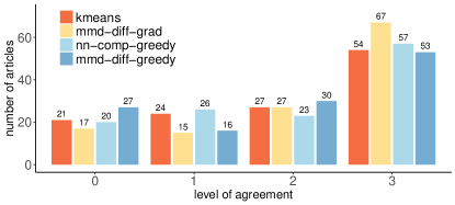
Figure 7 shows the level of agreement across participants for each method. First we note that participants were frequently able to complete the task of classifying new articles correctly into one of two groups, this is shown by the large fraction of articles for which the correct group was unanimously chosen. Compared to other comparative prototype selection methods mmd-diff-grad has the largest number of articles correctly classified by all three participants, beating the next best nn-comp-greedy by 10 articles. Consequently mmd-diff-grad also has fewer articles which were unanimously assigned to the incorrect group by participants.
Figure 8 shows the density plot comparing human accuracy vs. SVM accuracy in classifying small set of test articles we had for human evaluation.
Appendix E Results Table
Automatic evaluation results table corresponding to error-bar plot in Figure 4 is given in Tables 6, 6, 6 and 6, We report the mean of balanced accuracy and 95% confidence interval of the 10 random splits. The left four columns use 1-NN and the right four use SVM. We report results on 2, 4, 8, or 16 prototypes per group. The highest performing method is in bold and second highest performing one is in italics.
| method | 2 | 4 | 8 | 16 | 2 | 4 | 8 | 16 |
|---|---|---|---|---|---|---|---|---|
| kmedoids | 0.501 .010 | 0.505 .011 | 0.528 .012 | 0.530 .021 | 0.498 .008 | 0.501 .005 | 0.523 .014 | 0.523 .02 |
| kmeans | 0.510 .017 | 0.542 .012 | 0.546 .007 | 0.576 .008 | 0.507 .016 | 0.546 .009 | 0.541 .01 | 0.551 .012 |
| mmd-critic | 0.499 .003 | 0.514 .016 | 0.515 .013 | 0.531 .009 | 0.5 .001 | 0.499 .01 | 0.51 .017 | 0.53 .012 |
| mmd-diff-grad | 0.534 .011 | 0.538 .014 | 0.540 .020 | 0.582 .010 | 0.53 .011 | 0.542 .01 | 0.559 .012 | 0.575 .011 |
| mmd-div-grad | 0.539 .013 | 0.545 .008 | 0.564 .014 | 0.579 .011 | 0.527 .012 | 0.546 .014 | 0.56 .012 | 0.579 .009 |
| nn-comp-greedy | 0.509 .011 | 0.515 .008 | 0.544 .009 | 0.577 .007 | 0.517 .018 | 0.529 .015 | 0.56 .007 | 0.577 .006 |
| mmd-diff-greedy | 0.530 .009 | 0.536 .012 | 0.545 .013 | 0.564 .013 | 0.529 .014 | 0.554 .012 | 0.553 .012 | 0.575 .011 |
| mmd-div-greedy | 0.530 .010 | 0.525 .011 | 0.539 .012 | 0.563 .009 | 0.532 .014 | 0.544 .013 | 0.544 .007 | 0.578 .011 |
| method | 2 | 4 | 8 | 16 | 2 | 4 | 8 | 16 |
|---|---|---|---|---|---|---|---|---|
| kmedoids | 0.592 .016 | 0.586 .011 | 0.582 .025 | 0.589 .023 | 0.573 .022 | 0.571 .013 | 0.574 .025 | 0.578 .031 |
| kmeans | 0.582 .020 | 0.613 .017 | 0.622 .030 | 0.629 .025 | 0.57 .024 | 0.608 .022 | 0.615 .02 | 0.637 .027 |
| mmd-critic | 0.541 .031 | 0.524 .028 | 0.530 .025 | 0.535 .033 | 0.531 .028 | 0.533 .021 | 0.516 .039 | 0.542 .029 |
| mmd-diff-grad | 0.595 .019 | 0.587 .023 | 0.610 .017 | 0.633 .020 | 0.592 .036 | 0.612 .022 | 0.615 .024 | 0.641 .019 |
| mmd-div-grad | 0.602 .021 | 0.605 .015 | 0.605 .028 | 0.636 .028 | 0.595 .019 | 0.597 .025 | 0.608 .026 | 0.636 .019 |
| nn-comp-greedy | 0.587 .018 | 0.600 .027 | 0.624 .029 | 0.627 .026 | 0.588 .02 | 0.605 .014 | 0.615 .023 | 0.639 .026 |
| mmd-diff-greedy | 0.592 .027 | 0.595 .021 | 0.615 .019 | 0.629 .021 | 0.596 .019 | 0.597 .022 | 0.626 .021 | 0.642 .021 |
| mmd-div-greedy | 0.586 .014 | 0.578 .021 | 0.593 .022 | 0.616 .025 | 0.594 .019 | 0.583 .026 | 0.597 .027 | 0.632 .024 |
| method | 2 | 4 | 8 | 16 | 2 | 4 | 8 | 16 |
|---|---|---|---|---|---|---|---|---|
| kmedoids | 0.501 .016 | 0.504 .012 | 0.518 .016 | 0.518 .013 | 0.502 .014 | 0.502 .007 | 0.516 .011 | 0.52 .006 |
| kmeans | 0.505 .009 | 0.506 .006 | 0.538 .013 | 0.542 .014 | 0.508 .007 | 0.504 .01 | 0.527 .01 | 0.536 .008 |
| mmd-critic | 0.506 .006 | 0.511 .013 | 0.507 .011 | 0.514 .014 | 0.507 .007 | 0.504 .012 | 0.518 .018 | 0.518 .011 |
| mmd-diff-grad | 0.531 .009 | 0.529 .006 | 0.532 .008 | 0.566 .006 | 0.541 .008 | 0.528 .011 | 0.535 .009 | 0.554 .016 |
| mmd-div-grad | 0.525 .011 | 0.525 .009 | 0.537 .010 | 0.563 .011 | 0.532 .013 | 0.53 .012 | 0.54 .011 | 0.553 .014 |
| nn-comp-greedy | 0.502 .010 | 0.518 .011 | 0.535 .014 | 0.555 .009 | 0.515 .01 | 0.528 .011 | 0.528 .009 | 0.543 .009 |
| mmd-diff-greedy | 0.524 .015 | 0.520 .013 | 0.521 .013 | 0.537 .010 | 0.521 .017 | 0.529 .016 | 0.536 .013 | 0.55 .011 |
| mmd-div-greedy | 0.517 .012 | 0.515 .010 | 0.519 .012 | 0.532 .011 | 0.506 .01 | 0.531 .012 | 0.528 .013 | 0.55 .012 |
| method | 2 | 4 | 8 | 16 | 2 | 4 | 8 | 16 |
|---|---|---|---|---|---|---|---|---|
| kmedoids | 0.805 .010 | 0.836 .014 | 0.862 .008 | 0.881 .008 | 0.783 .009 | 0.845 .01 | 0.886 .005 | 0.907 .009 |
| kmeans | 0.823 .012 | 0.866 .010 | 0.888 .006 | 0.909 .009 | 0.815 .014 | 0.869 .011 | 0.901 .006 | 0.924 .009 |
| mmd-critic | 0.560 .019 | 0.700 .016 | 0.777 .013 | 0.839 .010 | 0.48 .037 | 0.63 .035 | 0.795 .022 | 0.877 .007 |
| mmd-diff-grad | 0.811 .011 | 0.852 .008 | 0.882 .007 | 0.910 .010 | 0.831 .013 | 0.877 .008 | 0.9 .011 | 0.922 .007 |
| mmd-div-grad | 0.806 .010 | 0.849 .010 | 0.876 .007 | 0.907 .010 | 0.834 .015 | 0.877 .009 | 0.901 .011 | 0.919 .008 |
| nn-comp-greedy | 0.800 .011 | 0.859 .010 | 0.890 .009 | 0.914 .010 | 0.792 .009 | 0.856 .012 | 0.894 .008 | 0.924 .008 |
| mmd-diff-greedy | 0.783 .011 | 0.835 .009 | 0.871 .009 | 0.898 .010 | 0.801 .008 | 0.86 .009 | 0.892 .011 | 0.917 .01 |
| mmd-div-greedy | 0.784 .013 | 0.840 .010 | 0.866 .010 | 0.898 .007 | 0.798 .008 | 0.866 .012 | 0.895 .01 | 0.92 .009 |