Effect of non-equilibrium ionization on derived physical conditions of the high-$z$ intergalactic medium

Abstract

Non-equilibrium ionization effects are important in cosmological hydrodynamical simulations but are computationally expensive. We study the effect of non-equilibrium ionization evolution and UV ionizing background (UVB) generated with different quasar spectral energy distribution (SED) on the derived physical conditions of the intergalactic medium (IGM) at $2\leq z\leq 6$ using our post-processing tool “Code for Ionization and Temperature Evolution” (cite). cite produces results matching well with self-consistent simulations more efficiently. The  He ii reionization progresses more rapidly in non-equilibrium model as compared to equilibrium models. The redshift of  He ii reionization strongly depends on the quasar SED and occurs earlier for UVB models with flatter quasar SEDs. During this epoch the normalization of temperature-density relation, $T_{0}(z)$, has a maximum while the slope, $\gamma(z)$, has a minimum, but occurring at different redshifts. The $T_{0}$ is higher in non-equilibrium models using UVB obtained with flatter quasar SEDs. While our models produce the observed median  He ii effective optical depth evolution and its scatter for equilibrium and non-equilibrium considerations, to explain the observed cumulative distributions we may need to consider fluctuating UVB. For a given UVB model, the redshift dependence of the  H i photo-ionization rate derived from the observed  H i effective optical depth ($\tau_{\rm eff,HI}$) for the equilibrium model is different from that for the non-equilibrium model. This may lead to different requirements on the evolution of ionizing emissivities of sources. We show that, in the absence of strong differential pressure smoothing effects, it is possible to recover the $T_{0}$ and $\gamma$ realised in non-equilibrium model from the equilibrium models generated by rescaling photo-heating rates while producing the same $\tau_{\rm eff,HI}$.

1 Introduction

The  H i  Ly$\alpha$ forest absorption seen in the spectra of distant quasars in conjunction with cosmological hydrodynamical simulations enable one to not only constrain cosmological parameters (Weinberg et al., 1998; McDonald et al., 2000; Penton et al., 2000; Phillips et al., 2001; McDonald et al., 2005; Viel et al., 2004; Shull et al., 2012b) but also probe the thermal and ionization history of the intergalactic medium (IGM, Schaye et al., 2000; Faucher-Giguère et al., 2008b; Lidz et al., 2010; Becker et al., 2011; Becker & Bolton, 2013). The outputs of a cosmological hydro-simulation depend on various ingredients such as (i) the assumed nature of ionizing background, (ii) implementation of various feedback processes and (iii) assumptions involved in the computations of thermal and ionization state of the gas. It is usually assumed that the IGM is in ionization equilibrium with uniform ionizing background dominated by quasars and galaxies. While most of these assumptions are valid for IGM in the post reionization era, they may not reflect the reality when reionization is in progress or just completed (Puchwein et al., 2015, 2019).

We have enough observational evidences to suggest that the  H i reionization was completed around $z\sim 5.5$ (Fan et al., 2001, 2006; Planck Collaboration et al., 2014). The  He ii  Ly$\alpha$ effective optical depth, measured towards rare UV bright quasars using Hubble Space Telescope (HST), shows a strong evolution over $2.7\leq z\leq 4.0$ and a much smaller scatter at $z<2.7$ (Jakobsen et al., 1994; Heap et al., 2000; Kriss et al., 2001; Shull et al., 2004; Fechner et al., 2006; Worseck et al., 2011; Worseck et al., 2018). These observations are consistent with the IGM going through two major reionization episodes with  He ii reionization being completed around $z\sim 2.7$, most likely driven by luminous quasars. In such a scenario one expects a fresh influx of thermal energy and entropy into the IGM at $2.7\leq z\leq 4.0$. Interestingly, the nature of  He ii reionization can also be probed using well measured properties of  H i  Ly$\alpha$ forest which can be easily accessed through ground based large telescopes. In particular one can use (i) the redshift evolution of temperature-density relation in IGM which is driven by residual photo-heating from  He ii ionization that systematically broadens the  H i absorption lines (Schaye et al., 2000; Theuns et al., 2002; Bolton et al., 2008; Lidz et al., 2010; Becker et al., 2011; Garzilli et al., 2012; Boera et al., 2014; Rudie et al., 2012; Hiss et al., 2018; Walther et al., 2019) and (ii) the presence or absence of structures in the redshift evolution of mean  H i  Ly$\alpha$ effective optical depth as a function of $z$ (Bernardi et al., 2003; Faucher-Giguère et al., 2008b; Becker et al., 2013).

Interpretations of IGM observations will crucially depend on assumptions related to basic ingredients of the cosmological simulations. In this work we investigate how the physical properties of the high-$z$ IGM is affected by (i) the allowed range in the  He ii photoionization rate ($\Gamma_{\rm HeII}$) for a given  H i photoionization rate ($\Gamma_{\rm HI}$) originating from the uncertainties in UV spectral energy distributions of quasars and (ii) the non-equilibrium effects in the calculations of ionization and thermal history of the gas.

The redshift evolution of cosmic ultra-violet radiation background (UVB) is computed by solving a 1D radiative transfer of extreme UV photons emitted by sources (such as galaxies and quasars), and attenuated by the foreground gas in IGM (Haardt & Madau, 1996; Faucher-Giguère et al., 2008a; Haardt & Madau, 2012; Khaire & Srianand, 2015a, 2019; Puchwein et al., 2019). The UV emissivity of quasars in the energy range relevant for  He ii reionization is highly uncertain due to uncertainties in mean spectral energy distribution of quasars (Khaire, 2017; Khaire & Srianand, 2019). Since quasars are main sources of  He ii ionizing photons, any uncertainty in its spectral energy distribution (specially in the extreme UV to soft X-ray range) can lead to uncertainties in the derived IGM parameters.

The thermal and ionization evolution of IGM in most of the hydrodynamical simulations are computed assuming the photo-ionization equilibrium. However, it takes some time for a parcel of gas, that got heated recently by the ionization of  He ii, to reach a new equilibrium. If the heating rate is faster than the time required for the gas to reach the photo-ionization equilibrium then the gas parcel will remain in a non-equilibrium state for a prolonged period of time. In such a cases it will be more appropriate to consider non-equilibrium ionization evolution (see Puchwein et al., 2015, 2019). However, for a given UVB, the hydrodynamic simulation incorporating non-equilibrium ionization evolution is expensive than a corresponding simulation performed using equilibrium consideration. Here we are exploring an approach that will allow us to study the effect of UVB and non-equilibrium evolution considering a wide range of parameter space in a computationally economical way.

In Gaikwad et al. (2017), we have developed an efficient method to simulate the effect of UVB on ionization and thermal evolution of the IGM in the post-processing step of gadget-2 (i.e., hydrodynamical simulation without radiative processes) using a module “Code for Ionization and Temperature Evolution” (cite). It was shown that most statistical distributions of IGM can be reproduced within 20 percent uncertainty compared to self-consistent gadget-3 simulations when we consider signal-to-noise, spectral resolution and total redshift pathlength typically achieved in real observations. In this work, we implement the non-equilibrium ionization evolution in cite (see §2) and study its effect on  He ii reionization for a range of UVB models obtained by varying quasar spectral indices.

This paper is organised as follows. In section 2, we provide basic details of our simulations, implementations of equilibrium and non-equilibrium calculations and various UVBs considered in this study. In section 3, we provide detailed comparisons of our simulations with those from the literature, study differences in the evolution of physical quantities in the non-equilibrium and equilibrium calculations and discuss the implications of using equilibrium simulations to extract IGM parameters when the actual evolution is governed by non-equilibrium processes. We summarize our results in section 4.

Throughout this work we use flat $\Lambda$CDM cosmology with parameters $(\Omega_{\Lambda},\Omega_{m},\Omega_{b},\sigma_{8},n_{s},h,Y)=(0.69,0.31,0.0486,0.83,0.96,0.674,0.24)$ consistent with Planck Collaboration et al. (2014). All distances are given in comoving units unless specified. $\Gamma_{\rm HI}$ expressed in units of $10^{-12}\>{\rm s}^{-1}$ is denoted by $\Gamma_{\rm 12}$.

2 Simulation

The high resolution simulations used in this work were run using the publicly available smooth particle hydrodynamics code gadget-2 (Springel, 2005) with initial conditions generated at redshift $z=99$ using the publicly available 2lpt code (Scoccimarro et al., 2012). Our default simulation has a box size of $L_{\rm box}=10h^{-1}$  cMpc, number of particles $N_{\rm particle}=512^{3}$ and gas mass resolution, $m_{\rm gas}\sim 10^{5}\>\rm M_{\odot}$. We set gravitational softening length as 1/30^th of the inter particle distance. We store the outputs from $z=6$ to $z=1.6$ in steps of $\Delta z=0.1$ to track the density and temperature evolution of particles.

The publicly available version of gadget-2 neither solves the ionization evolution equations nor incorporates the radiative heating or cooling. As a result, the temperature of low density unshocked gas (high density shocked gas) in gadget-2 is lower (higher) than that expected in a self-consistent simulation. An updated version of gadget-2, known as gadget-3, solves the ionization and thermal evolution equations for a given UVB model self-consistently (Springel, 2005). However, performing gadget-3 simulations for a wide range of UVB models is computationally expensive (see, e.g., Table 6 in Gaikwad et al., 2018). Also, the default version of gadget-3 solves the evolution equations assuming ionization equilibrium (but see Puchwein et al., 2015, 2019, where non-equilibrium ionization evolution has been incorporated within gadget-3).

To account for the above issues, we have developed a post-processing module called “Code for Ionization and Temperature Evolution” (cite) which can be used to incorporate the radiative heating and cooling such that one will be able to mimic various physical effects present in the simulations (such as pressure broadening) within few percent accuracy (Gaikwad et al., 2017, 2018). In Gaikwad et al. (2018, here after G18), we have shown that cite is flexible, efficient and can reproduce results consistent with self-consistent gadget-3 simulations for equilibrium ionization evolution. Further, it also allows us to model the non-equilibrium ionization and thermal evolution. It has been shown in G18 that the most accurate results (when compared to a full gadget-3 runs) are obtained when gadget-2 is run with elevated temperature floor of $10^{4}$ K, motivated by the fact that the typical temperature of photo-ionized IGM is few times $10^{4}$ K (at overdensity of $\Delta=1$, Hui & Gnedin, 1997).

In the redshift range of our interest ($2\leq z\leq 6$), the  He ii ionizing UVB can have large spatial fluctuations (Furlanetto & Oh, 2008; Dixon et al., 2014; La Plante & Trac, 2016; La Plante et al., 2017, 2018; Davies et al., 2017) as one is most likely probing the end stages of  He ii reionization. These fluctuations arise mainly because the mean free path of  He ii ionizing photons is smaller than the mean separation between the quasars. However, in this work we use UVB from synthesis models which implicitly assume that the UVB is spatially uniform (but is evolving with time). This, combined with the fact that our simulation box is too small to capture properties of individual  He iii region around a typical bright quasar, implies that we do not account for the patchy  He ii reionization process. We assume instead that the filling fraction of  He iii regions and the  $f_{\rm HeIII}$ in our simulation box are equivalent (Puchwein et al., 2015, here after P15). Furthermore, the heating rate during  He ii reionization depends not only on the nature of UVB but also on the speed of the ionization front in IGM (D’Aloisio et al., 2018). On the other hand, our simulation can resolve  H i  Ly$\alpha$ forest at the thermal broadening scales and has the resolution consistent with that has been typically used in the echelle spectroscopy for studying the  Ly$\alpha$ forest.

2.1 Temperature and Ionization Evolution Equation

The thermal evolution of IGM is governed by following equation (Hui & Gnedin, 1997; Gaikwad et al., 2017, 2018),

$$\frac{dT}{dt} = -2HT+\frac{2T}{3\Delta}\>\frac{d\Delta}{dt}+\frac{dT_{shock}}{dt}+\frac{T}{\sum\limits_{X}f_{\rm X}}\>\frac{d\sum\limits_{\rm X}f_{\rm X}}{dt}$$ (1)

$$+ \frac{2}{3\>k_{B}\>n_{b}}\;(\mathscr{H}-\mathscr{C})$$

where $H$, $k_{B}$, $\Delta$ and $n_{b}$ are Hubble parameter, Boltzmann constant, overdensity and number density of baryons respectively. The symbol $f_{\rm X}\equiv n_{\rm X}/n_{\rm H}$ where $n_{\rm X}$ and $n_{H}$ are number densities of species $X\in[$ H i, H ii,  He i,  He ii,  He iii, $e]$ and hydrogen respectively. $\mathscr{H}$ and $\mathscr{C}$ are the total heating and cooling rates per unit volume (${\rm ergs\;cm^{-3}\;s^{-1}}$) respectively. The five terms on the right hand side of the above equation, respectively, represent rate of change of temperature due to, (i) Hubble expansion, (ii) adiabatic heating or cooling, (iii) shock heating from structure formation, (iv) change in internal energy and (v) radiative heating or cooling processes. The first three terms on the right hand side of the above equation are computed self-consistently in gadget-2. The last two terms are calculated in cite for each particle by solving the following set of ionization evolution equations assuming primordial composition (H and He only) of gas,

$$\alpha_{\text{HII}}\>n_{e}\>f_{\rm HII}-f_{\rm HI}\>(\Gamma^{\gamma}_{{\rm H\textsc{i}}}+\Gamma^{\rm e}_{{\rm H\textsc{i}}}\>n_{e}) =\frac{df_{\rm HI}}{dt}$$ (2)

$$\alpha_{\text{HeII}}\>n_{e}\>f_{\rm HeII}-f_{\rm HeI}\>(\Gamma^{\gamma}_{{\rm He\textsc{i}}}+\Gamma^{\rm e}_{{\rm He\textsc{i}}}\>n_{e}) =\frac{df_{\rm HeI}}{dt}$$

$$-\alpha_{\text{HeIII}}\>n_{e}\>f_{\rm HeIII}+f_{\rm HeII}\>(\Gamma^{\gamma}_{{\rm He\textsc{ii}}}+\Gamma^{\rm e}_{{\rm He\textsc{ii}}}\>n_{e}) =\frac{df_{\rm HeIII}}{dt}$$

$$f_{\rm HI}+f_{\rm HII} =1$$

$$f_{\rm HeI}+f_{\rm HeII}+f_{\rm HeIII} =y$$

$$f_{\rm HII}+f_{\rm HeII}+2f_{\rm HeIII} =f_{\rm e}$$

where $\Gamma^{\gamma}_{{X_{i}}}$, $\Gamma^{\rm e}_{{X_{i}}}$, $\alpha_{X_{i}}(T)$ and $n_{\rm e}$ are photoionization rate, collisional ionization rate, recombination rate coefficient and number density of electrons respectively. The fraction $y=Ym_{\rm H}/[m_{\rm He}\>(1-Y)]$ is He abundance by number where $m_{\rm H},m_{\rm He}$ are the atomic mass of H, He and $Y$ is He abundance by mass respectively. We use collisional ionization and recombination rates from Theuns et al. (1998). The term $\mathscr{C}$ and $\mathscr{H}$ can be calculated by summing the cooling rates (Katz et al., 1996; Theuns et al., 1998, see their Table B1) and heating rates as given by,

$$\mathscr{H} = \;(f_{\rm HI}\>\epsilon_{\gamma{\rm HI}}\;+\;f_{\rm HeI}\>\epsilon_{\gamma{\rm HeI}}\;+\;f_{\rm HeII}\>\epsilon_{\gamma{\rm HeII}})/n_{\rm H}$$

$$\mathscr{C} = \sum\limits_{k=1}^{11}\;c_{k}(T,z,{X_{i}})$$ (3)

where $\epsilon_{\gamma{\rm X}}$ is photo-heating rates for species $X\equiv[{\rm H\textsc{i}},{\rm He\textsc{i}},{\rm He\textsc{ii}}]$ and $c_{k}(T_{,}z,{X_{i}})$ is cooling rate coefficient for all the relevant cooling processes such as collisional ionization, recombination, dielectronic recombination, collisional excitation, Bremsstrahlung and inverse Compton cooling. We use $c_{k}(T_{,}z,{X_{i}})$ consistent with that from Theuns et al. (1998, see Table B1). The photoionization and photo-heating rates are obtained from the assumed uniform UVB model. We also use the rate coefficients as given in Lukić et al. (2015) and find that the maximum difference in the results are less than 8 percent.

2.2 Equilibrium and Non-equilibrium Ionization Evolution

In the simulation runs using the default version of gadget-3, Eq. 2 is solved for equilibrium ionization conditions i.e., setting right hand side of the first three relations in Eq. 2 to zero and excluding the explicit time dependence of ionization fraction (exceptions being Puchwein et al., 2015, 2019). In our case, to solve equilibrium ionization evolution equations (at any $z$) numerically, we start with an initial guess value for electron number density ($n_{e}\sim n_{H}$). We then solve the set of simultaneous equations (first $5$ equations in Eq. 2) to compute the ionization fraction for different states of H and He. We use the last relation in Eq. 2 to update the value of electron number density $n_{e}$. The recombination rates ($\alpha_{\rm X}$) depend on the temperature and we use the updated temperatures at each time step to compute the ionization fractions accurately. We repeat the process with updated value of $n_{e}$ until the values of all the variables converge to an absolute tolerance of $10^{-7}$.

Using equilibrium solutions, however, may not be a good approximation if the time scales of radiative processes (recombination or photo-ionization) become longer than the Hubble time or the time scale over which physical quantities like gas temperature evolve. In particular, such an approximation is not expected to be valid during  He ii (or  H i) reionization since it takes some time for an ionized parcel of gas to reach a new ionization equilibrium.

The non-equilibrium solutions to Eq. 2 is non-trivial as the explicit time dependent equations (first three relations in Eq. 2) tend to be stiff owing to the different time scales involved in the problem. We solve the non-equilibrium ionization evolution equation (Eq. 2) using Sundials CVODE library (python version) (Cohen et al., 1996; Oppenheimer & Schaye, 2013; Puchwein et al., 2015). This library integrates the set of stiff ordinary differential equations with variable-order, variable-step using Backward Differentiation Formula (BDF) methods. We use the relative error tolerance of $10^{-7}$ for various ionization fractions of H and He in CVODE library.

It is important to note that the equilibrium or non-equilibrium models discussed in this work refers to the nature of the ionization evolution of the gas in IGM. In both models, we solve temperature evolution equation with explicit time dependence that is we account for $dT/dt$ term on left hand side of Eq. 1.

The difference between equilibrium and non-equilibrium ionization evolution of  He ii could affect the changes in electron number density and thermal history of the IGM. As the contribution of  He ii to the number density of electrons is small ($n_{\rm H}/n_{\rm He}\sim 12$), change in $n_{e}$ due to reionization of  He ii does not influence the ionization state of  H i significantly. However, the effect on the thermal history of the IGM could be significant depending on whether one uses equilibrium and non-equilibrium ionization evolution. Since the recombination rate depends on the temperature of the IGM, the ionization state of  H i can be affected significantly (see Eq. 2). In addition, the pressure smoothing effects are also expected to be significantly different between equilibrium and non-equilibrium ionization evolution. Keeping this in mind, our main aim in this work is to explore the effect of equilibrium and non-equilibrium ionization evolution (i) on thermal history of IGM, (ii) on the derived  H i photo-ionization rate $\Gamma_{\rm HI}$ at $2<z<4$ and (iii) on the redshift evolution of  He ii effective optical depth. We will discuss these issues in detail in §3.

2.3 UVB Models

The main inputs for the cite and our non-equilibrium calculations are the photoheating and photoionization rates obtained from the UVB synthesis models. In such synthesis models, the UVB at any redshift $z_{0}$ is obtained by solving the radiative transfer of extreme UV photons emitted by sources (quasars and galaxies) and filtered by the gas in IGM at all $z>z_{0}$ (see e.g Haardt & Madau, 1996; Faucher-Giguère et al., 2008a; Haardt & Madau, 2012; Khaire & Srianand, 2015a, 2019; Puchwein et al., 2019). The UV emissivities of sources are obtained by using the observed luminosity functions at a single rest wavelength combined with their mean spectral energy distribution (SED). However, these emissivity estimates are highly uncertain because (i) there are very little observational constraints on either ionizing emissivities or the SED of galaxies in the relevant energy ranges, (ii) there is no consensus on the ionizing SED of quasars (see table 1 of Khaire, 2017), and (iii) the faint end slopes and the limiting magnitudes of quasars and galaxies, to be used while integrating the luminosity functions to obtain emissivities are not well constrained at $z>3$ (Giallongo et al., 2015; Khaire & Srianand, 2015b; Khaire et al., 2016; Kulkarni et al., 2018). To partially circumvent the emissivity uncertainties, the UVB synthesis models usually tune the unconstrained ionizing emissivity from galaxies in order to match with the observed  H i photoionization rates. This is performed by changing escape fraction ($f_{\rm esc}$) of  H i ionizing photons from galaxies under the assumption that the SED of galaxies is determined by stellar population synthesis models and extinction by dust. It is also usually assumed that galaxies with typical stellar populations (i.e population II) do not contribute significantly to high energy photons that can ionize  He ii (Dayal & Ferrara, 2018).

Unfortunately, fixing the  He ii ionizing emissivity of quasars for $E>54.4$ eV is also difficult as quasar SEDs are not measured in these energy ranges and constraints on  He ii photoionization rates obtained from high-z IGM are just beginning to emerge (for e.g., Khaire, 2017; Worseck et al., 2018). To overcome this issue in  He ii ionizing UVB, we use the allowed range of UVB models presented in Khaire & Srianand (2019, here after KS19) obtained with different  He ii ionizing emissivities. In KS19, the quasar emissivity at non-ionizing wavelengths (Far UV) is taken from the updated estimates by Khaire & Srianand (2015a) and the ionizing emissivity is obtained by varying quasar SED using allowed range of power law indices. The measurements of quasar SEDs are obtained by fitting power law relation ($f_{\nu}\propto\nu^{-\alpha}$) to the stacked mean ionizing spectrum of quasars (at $E>13.6$ eV). The recent measurements of such power law index $\alpha$ has been reported to have values from $0.7$ to $2.5$ (Shull et al., 2012b; Stevans et al., 2014; Lusso et al., 2015; Tilton et al., 2016; Lusso et al., 2018). In this work, we have used four UVB models calculated using $\alpha$ in the range of $1.4$ to $2.0$ with the interval of $0.2$ (Khaire & Srianand, 2019). In addition to these four UVB models we also use Haardt & Madau (2012, here after HM12 that used $\alpha=1.57$) UVB for comparison with results of P15.

In order to facilitate easy identification of models, we refer to them using nomenclatures as identified in first column of Table 1. Model NE-KS19-2.0 refers to non-equilibrium ionization evolution of gas exposed to KS19 UVB with quasar SED obtained using a power law index of $\alpha=2.0$. The model EQ-KS19-1.4 corresponds to the equilibrium ionization evolution for KS19 UVB with quasar SED having $\alpha=1.4$. All models listed in Table 1 are obtained by post-processing gadget-2 simulation ($L_{\rm box}=10h^{-1}$  cMpc, $N_{\rm particle}=512^{3}$, see §2) with cite.

Table 1: Details of models studied in this work. Same for additional models discussed in this work are given in the Appendix A

Model Namea	Codeb	Ionization evolution	UVB	Quasar spectral index ($\alpha$)c	Reference
EQ-KS19-1.4	gadget-2 + cite	equilibrium	KS19	1.4	This work
NE-KS19-1.4	gadget-2 + cite	Non-equilibrium	KS19	1.4	This work
EQ-KS19-2.0	gadget-2 + cite	equilibrium	KS19	2.0	This work
NE-KS19-2.0	gadget-2 + cite	Non-equilibrium	KS19	2.0	This work
EQ-HM12	gadget-2 + cite	equilibrium	HM12	1.57	This work
NE-HM12	gadget-2 + cite	Non-equilibrium	HM12	1.57	This work
EQ-HM12-G18	gadget-3	equilibrium	HM12	1.57	Gaikwad et al. (2018)
NE-HM12-P15d	gadget-3	Non-equilibrium	HM12	1.57	Puchwein et al. (2015)

• In the main text of this paper, we present the results of total $4$ different models. We refer readers to appendix for additional $16$ models analysed in this work. In the appendix, these models are referred with prefix L10-N512-G2 (L10-N512 model performed using gadget-2 + cite) attached to the model name. For example, the model EQ-KS19-1.4 is referred as L10-N512-G2-EQ-KS19-1.4. All simulation outputs were store from $z=6$ to $z=1.6$ in steps of $\Delta z=0.1$ (except NE-HM12-P15).

• gadget-2 simulation is performed with $L_{\rm box}=10h^{-1}$  cMpc, $N_{\rm particle}=2\times 512^{3}$ (L10-N512) and gas mass resolution $\delta m\sim 10^{5}\>\rm M_{\odot}$. Post-processing module cite is applied on gadget-2 output. cite provides flexibility to change UVB and perform equilibrium / non-equilibrium ionization evolution efficiently.

• The UVB models are generated by varying the uncertain quasar spectral slopes $\alpha$, defines as $f_{\nu}\propto\nu^{-\alpha}$ KS19. We vary $\alpha$ from 1.4 to 2.0 in steps of 0.2.

• NE-HM12-P15 simulations are performed with $L_{\rm box}=20h^{-1}$  cMpc, $N_{\rm particle}=2\times 512^{3}$ (see, Puchwein et al., 2015).

3 Result

3.1 Comparison between equilibrium and non-equilibrium models

We first present our results on how the IGM properties depend on whether we are solving the Eq. 2 using the equilibrium approximation or taking into account the explicit time evolution. We also demonstrate how well our post-processing approach (cite) captures all the basic results seen in self-consistent simulations.

3.1.1 Evolution of  H i and  He ii fraction

The evolution of  H i and  He ii fractions are important for understanding the effect of UVB on ionization state of the IGM. Furthermore, the excess kinetic energy carried away by electrons is responsible for changing the thermal state of IGM during reionization. The amount of photo-heating is directly proportional to the  H i and  He ii fractions (see Eq. 2.1). We define a volume average  H i and  He ii fraction in following way (Puchwein et al., 2015)

$$f_{\rm HI}=\frac{n_{\rm HI}}{n_{\rm H}}\;\;\;{\rm and}\;\;\;f_{\rm HeII}=\frac{n_{\rm HeII}}{(n_{\rm HeI}+n_{\rm HeII}+n_{\rm HeIII})}$$ (4)

where $n_{\rm X}$ is volume average number density of a species X.

Figure 1: Left panel shows the comparison of volume averaged  $f_{\rm HI}$ and  $f_{\rm HeII}$ evolution for equilibrium model from this work (EQ-HM12,  $f_{\rm HI}$ in magenta dashed-dotted line,  $f_{\rm HeII}$ in blue solid line) with that from self-consistent models derived in G18 (EQ-HM12-G18,  $f_{\rm HI}$ in green dotted line,  $f_{\rm HeII}$ in red dashed line). The  $f_{\rm HI}$ and  $f_{\rm HeII}$ evolution in two models are in good agreement. Right panel is similar to left panel except the comparison is shown for non-equilibrium models where we compare the  $f_{\rm HI}$ and  $f_{\rm HeII}$ evolution in this work with that from P15 ( $f_{\rm HI}$ in green dotted line,  $f_{\rm HeII}$ in red dashed line). The small mismatch between the two models is mostly due to the differences in the rate coefficients and cosmological parameters (simulation box size and number of particles are same). All the curves are shown for Haardt & Madau (2012) UVB model.

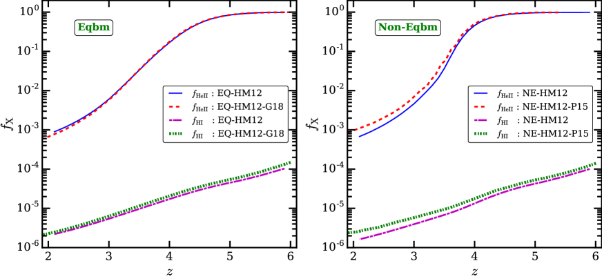
We show the  $f_{\rm HeII}$ and  $f_{\rm HI}$ evolution for equilibrium (left panel) and non-equilibrium (right panel) models using gadget-2 + cite with HM12 UVB in Fig. 1. We also show the same two quantities obtained using an equilibrium gadget-3 simulation (EQ-HM12-G18), identical to that used in G18, in the left panel of Fig. 1. Finally, we compare the  $f_{\rm HeII}$ and  $f_{\rm HI}$ evolution from our calculations with those obtained from the gadget-3 simulations of P15 (NE-HM12-P15) in the right panel in Fig. 1. We remind the readers that the  $f_{\rm HeII}$ and  $f_{\rm HI}$ evolution in NE-HM12-P15 model is calculated self-consistently by solving the non-equilibrium ionization evolution equations in the gadget-3 code.

From the left panel of the figure, we find that ion fractions obtained using our implementation of the equilibrium model matches within 14 percent with that of the gadget-3 simulations. Similarly, we find a good agreement between results of our non-equilibrium model (NE-HM12) and the models of P15 (NE-HM12-P15) as can be seen from the right panel of the figure. The difference between the two non-equilibrium models is within $\sim 20$ percent and major contribution to this can be attributed to the differences in the rate coefficients, cosmology and non-equilibrium solver used in this work and P15. Note that  $f_{\rm HeII}$ is the main quantity governing the ionization and thermal evolution of IGM at $2\leq z\leq 6$. Since  $f_{\rm HeII}$ evolution for equilibrium and non-equilibrium models obtained using gadget-2 + cite match with those obtained from full gadget-3 runs, the thermal evolution in these models are also consistent with each other. The consistency of the thermal evolution for equilibrium and non-equilibrium models with that from gadget-3 ( P15, for non-equilibrium model) has already been shown in Fig. 4 of G18.

Thus, Fig. 1 validates our implementation of equilibrium and non-equilibrium ionization evolution in cite. In particular, the agreement of  $f_{\rm HeII}$ evolution at 20 percent level between P15 and our implementation is important for modelling the IGM at $2\leq z\leq 6$. As we will show later the differences in  $f_{\rm HeII}$ evolution between equilibrium and non-equilibrium calculations are much higher than the difference we find between exact calculations of non-equilibrium  $f_{\rm HeII}$ and our calculations using cite.

The left (right) panel of Fig. 2 shows the evolution of  $f_{\rm HeII}$ ( $f_{\rm HI}$) for two different KS19 UVB models with $\alpha=1.4$ and $2.0$ respectively. From the left panel, we see that  $f_{\rm HeII}$ $\sim 1$ at high redshifts and decreases to $\sim 10^{-2}-10^{-3}$ around $z\sim 3$. As expected, the exact redshift of  He ii reionization (for example say when  $f_{\rm HeII}$ $\leq 0.025$) depends on our choice of $\alpha$; higher values of $\alpha$ provide lower  He ii ionizing emissivity delaying the redshift of  He ii reionization. This result is qualitatively similar to  $f_{\rm HeII}$ evolution obtained in Puchwein et al. (2019). In this analysis, we assume that $\alpha$ is not evolving with redshift. Any redshift dependence of $\alpha$ will complicate the redshift dependence of ion fractions and temperature.

Concentrating on the $\alpha=1.4$ case, we find that  $f_{\rm HeII}$ is consistently smaller for equilibrium model (EQ-KS19-1.4) than that for non-equilibrium model (NE-KS19-1.4) during  He ii reionization at $3.7<z<5$. This is because  $f_{\rm HeII}$ in the equilibrium model is equated to the recombinations at each time step (Puchwein et al., 2015). Since recombinations are proportional to $\Delta^{0.6}$ (see Eq. 5),  $f_{\rm HeII}$ in equilibrium models is decided by the instantaneous density of particles. On the other hand,  $f_{\rm HeII}$ in non-equilibrium model is decided by the  $f_{\rm HeII}$ in previous time step,  He ii photo-ionization rate ($\sim\Gamma^{-1}_{\rm HeII}$), the recombination time scale and the instantaneous density of gas. The photo-ionization and recombination time scales evolve with redshift due to the $\Gamma_{\rm HeII}$ and thermal evolution. Irrespective of our choice of $\alpha$, $f_{\rm HeII}$ is found to be larger in non-equilibrium models compared to that of equilibrium models prior to the epoch of  He ii reionization. This is probably related to a steep rise in gas temperature we see in the non-equilibrium models within a typical recombination time-scale. Once the  $f_{\rm HeII}$ becomes small enough ( $f_{\rm HeII}$ $\leq$ 0.025), we find that the ionization evolution is governed by the balance between photo-ionization and recombination. In the case of non-equilibrium models, having slightly higher temperatures, should result in lower  $f_{\rm HeII}$ than that for equilibrium model. This is what we see in Fig. 2. This trend seen in  He ii for post reionization epoch is also seen in the  $f_{\rm HI}$ evolution (right panel in Fig. 2). The redshift at which the photo-ionization equilibrium is reached is different for different UVB models. For example, for $\alpha=1.4$ and $2.0$ the redshifts are $z=3.7$ and $3.2$ respectively. Below these redshifts, the  $f_{\rm HeII}$ fraction for non-equilibrium is consistently smaller than that for equilibrium models.

Table 2: Extent of  He ii reionization

Model	$z_{\rm start}$a	$z_{\rm end}$b	$\Delta z$c
EQ-KS19-1.4	5.03	3.70	1.33
NE-KS19-1.4	4.60	3.70	0.90
EQ-KS19-2.0	4.50	3.20	1.30
NE-KS19-2.0	4.05	3.20	0.85

• $z_{\rm start}$ corresponds to the epoch when $f_{\rm HeII}=0.9$ see Fig.2

• $z_{\rm end}$ corresponds to the epoch when $f_{\rm HeII}=0.025$ see Fig.2

• $\Delta z=z_{\rm start}-z_{\rm end}$ represent extent of  He ii reionization.

The extent of  He ii reionization is different when non-equilibrium effects are taken into account. To quantify the differences in the extent of  He ii reionization, we assume that the  He ii reionization starts at redshift $z_{\rm start}$ corresponding to the epoch when $f_{\rm HeII}=0.9$ and it ends at redshift $z_{\rm end}$ when  $f_{\rm HeII}$ drops below $0.025$. This choice of $z_{\rm end}$ is motivated by the fact that equilibrium and non-equilibrium  $f_{\rm HeII}$ cross each other at $f_{\rm HeII}=0.025$ irrespective of the UVB model we use. Table 2 summarizes the $z_{\rm start}$, $z_{\rm end}$ and redshift interval ($\Delta z$) for  He ii reionization for the UVB models shown in Fig. 2. The $z_{\rm start}$ is consistently lower for non-equilibrium models as compared to that from equilibrium model. As a result, the  He ii reionization in equilibrium case is more extended with $\Delta z\sim 1.3$. As we discussed earlier, the $z_{\rm start}$ and $z_{\rm end}$ are smaller for $\alpha=2.0$ than for $\alpha=1.4$ because of lower  He ii ionizing emissivity in the former case.

The right panel in Fig.2 shows evolution of  $f_{\rm HI}$ for models with $\alpha=1.4$ and 2.0. Even though non-equilibrium ionization evolution effects are important during  He ii reionization ($2\leq z\leq 4$), photo-ionization equilibrium for  H i is still a good approximation as  H i is highly ionized. The recombination rate required to maintain this highly ionized state can be achieved over a short time-scale. Therefore, at $z<5$,  $f_{\rm HI}$ is consistently smaller for non-equilibrium models than that for equilibrium model. The variation in  $f_{\rm HI}$ seen at $z<5$ is consistent with evolution of  $f_{\rm HeII}$ and temperature of IGM (also see Puchwein et al., 2015). The temperature of IGM is consistently larger for non-equilibrium models than that for corresponding equilibrium models at $z<5$ (see §3.1.3 for details). Since $f_{\rm HI}\propto T^{-0.7}$ for photo-ionization equilibrium, the  $f_{\rm HI}$ obtained in non-equilibrium model is consistently smaller.

Figure 2: Comparison of volume averaged  $f_{\rm HeII}$ (left panel) and  $f_{\rm HI}$ (right panel) evolution from KS19 for equilibrium and non-equilibrium ionization evolution. The evolutions of  $f_{\rm HI}$ and  $f_{\rm HeII}$ are shown for two KS19 UVBs compiled for two different quasar spectral indices ($\alpha=1.4$ and $2.0$). Comparison of EQ-KS19-2.0 (magenta diamonds) with NE-KS19-2.0 (green stars) in left panel shows that at $z>3.2$  $f_{\rm HeII}$ is under predicted in equilibrium case than that in non-equilibrium case. On the other hand at $z<3.2$,  $f_{\rm HeII}$ is lower in equilibrium case than that from non-equilibrium due to larger $T_{0}$. Comparison of NE-KS19-1.4 (blue squares) with NE-KS19-2.0 (green stars) shows that  $f_{\rm HeII}$ is larger for larger $\alpha$ (this is valid for equilibrium case also) indicating that redshift of  He ii reionization strongly depends on $\alpha$. Right panel shows that for a given UVB model, evolution of  $f_{\rm HI}$ is similar for equilibrium and non-equilibrium case at $z\geq 4.5$. However at $z<4.5$,  $f_{\rm HI}$ in the equilibrium case is consistently more than that for non-equilibrium case for a given UVB model. This is because $T_{0}$ (and  $f_{\rm HeII}$) in non-equilibrium model is systematically larger than that in equilibrium model at $z<4.5$ (See Fig. 4).

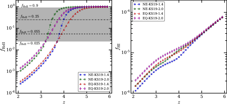
Another interesting effect to note from Fig. 2 is the appearance of a kink like feature at $z\sim 3.8$ in the  $f_{\rm HI}$ curve for EQ-KS19-1.4 model. Such a kink is not apparent in other cases. As we will see latter this is related to a sharp increase in temperature with $z$ seen in EQ-KS19-1.4 model. We come back to this in more detail in following sections.

3.1.2 Temperature-Density Relation

Figure 3: Left and right panels show the TDR for EQ-KS19-1.4 and NE-KS19-1.4 models respectively at $z=3.8$ (similar to Fig. 2 in P15). The color scheme shows the density of points in logarithmic scale. The power-law is fitted to TDR by calculating the median temperature (black stars) in $4$ $\log\Delta$ bins (shown by magenta dashed vertical lines). In both panels, the fitted power laws for equilibrium and non-equilibrium model are shown by dotted and dashed black lines respectively. The TDR is flatter ($\gamma$ is smaller) and has higher normalization ($T_{0}$) in non-equilibrium model as compared to equilibrium model. At $\log\Delta<-0.5$, the TDR deviates from power-law for non-equilibrium models. In each panel we also provide the best fit values of $T_{0}$ and $\gamma$. Our method of calculating $T_{0}$ and $\gamma$ is different than that from P15 (see §3.1.2 for details).

The low density IGM follows a power-law temperature-density relation (TDR) of the form $T=T_{0}\>\Delta^{\gamma-1}$ where $T_{0}$ and $\gamma$ are temperature of IGM at cosmic mean density ($\Delta=1$) and slope of TDR respectively (Hui & Gnedin, 1997). For a given simulation at redshift $z$, we calculate $T_{0}$ and $\gamma$ as follows,

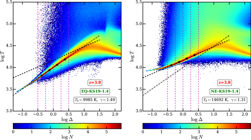
1. We collect the temperature of all the particles in different $\log\Delta$ bins centred at $[-0.375,-0.125,0.125$ and $0.375]$ having width of $0.25$. The choice of these bins is motivated by the fact that the TDR deviates from power-law at $\log\Delta<-0.5$ for non-equilibrium models (see Fig. 3) whereas the scatter in temperature is more at $\log\Delta>0.5$ for equilibrium and non-equilibrium models.

2. We then calculate the median temperature ($\log T$) of particles in each $\log\Delta$ bin.

3. Finally, we obtain best fit $T_{0}$ and $\gamma$ by fitting straight line, $\log T=\log T_{0}+(\gamma-1)~{}\log~{}\Delta$, to the median $\log T$ measured in each $\log\Delta$ bin.

Fig. 3 shows the comparison of TDR from the equilibrium (left panel) and non-equilibrium (right panel) models at $z=3.8$ for the KS19-1.4 UVB. As expected, most of the points follow a power law TDR in equilibrium and non-equilibrium cases. However at $\log\Delta<-0.5$, the TDR in non-equilibrium model is flattened. This deviation at $\log\Delta\leq-0.5$ from a single power law for non-equilibrium model occurs because  $f_{\rm HeII}$ in the non-equilibrium case does not only depend on the instantaneous density of particles (see Appendix B for details). As a result,  $f_{\rm HeII}$ at $\log\Delta<-0.5$ is higher in non-equilibrium models than that for equilibrium models. However in the equilibrium case,  $f_{\rm HeII}$ strongly depends on density since  He ii neutral fraction is directly set by number of recombinations and $f_{\rm HeII}\propto\Delta^{0.6}$ (see Eq. 5). The  $f_{\rm HeII}$ in EQ-KS19-1.4 and NE-KS19-1.4 are very similar at $z=3.8$ (see Fig 2). However $T_{0}$ is higher and $\gamma$ is smaller for the NE-KS19-1.4 model than the EQ-KS19-1.4 model. This can be attributed to the fact that the amount of energy injected over a small redshift range $\Delta z$ in the non-equilibrium case (NE-KS19-1.4) is more than that in the equilibrium case (EQ-KS19-1.4) as  $f_{\rm HeII}$ is higher in the former case. The behaviour of TDR for equilibrium and non-equilibrium models seen in our case are qualitatively similar to those from P15 (their Fig. 2). However,Our method of calculating $T_{0}$ and $\gamma$ is different from that used in P15. The $T_{0}$ in P15 corresponds to the median temperature of all gas particles with densities within 5 percent of $\Delta=1$. Whereas $\gamma$ in P15 is calculated by fitting a line between TDR at $(\Delta_{1}=10^{-0.5},T_{\rm median}(\Delta_{1}))$ and $(\Delta_{2}=1,T_{\rm median}(\Delta_{2}))$ where $T_{\rm median}(\Delta)$ is median temperature at $\Delta$.

3.1.3 Evolution of $T_{0}$ and $\gamma$

Figure 4: We show the evolution of $T_{0}$ and $\gamma$ from KS19 UVB compiled using two quasar spectral indices $\alpha=1.4$ and $\alpha=2.0$. For each UVB, $T_{0}$ and $\gamma$ evolution is shown for equilibrium and non-equilibrium ionization evolution. Equilibrium model produces lower $T_{0}$ as compared to that from non-equilibrium case at $z<5$. This is because  $f_{\rm HeII}$ is under predicted in equilibrium case as discussed in §3.1.3. (also see Fig. 2). On the other hand $\gamma$ is smaller for non-equilibrium models as compared to equilibrium models. This is due to the density independent photo-heating of the gas in non-equilibrium case. The vertical dashed lines in top panel and the vertical dashed-dotted lines bottom panel correspond to the redshift at which $d\log f_{\rm HeII}/dz$ and $df_{\rm HeII}/dz$ are maximum respectively (see Fig. 5) In all cite runs, we have assumed the initial $T_{0}$ ($=7920$ K) and $\gamma$ ($=1.55$) to be same at $z=6$.

Figure 5: Top panel shows the evolution of derivative of $\log f_{\rm HeII}$ with respect to $z$ (see Fig. 2). The peak in $d\log f_{\rm HeII}/dz$ correlates with peak in $T_{0}$ (dashed vertical lines) for all the UVB models (see Fig. 4). Bottom panel shows the evolution of derivative of $f_{\rm HeII}$ with respect to $z$. The peak in $df_{\rm HeII}/dz$ correlates with epoch of minimum $\gamma$ (dash-dotted vertical lines) for all the UVB models. Thus  $f_{\rm HeII}$ is a main driving factor affecting the $T_{0}$ and $\gamma$ evolution (see Fig. 4).

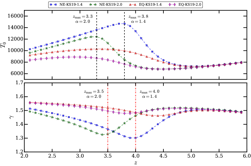
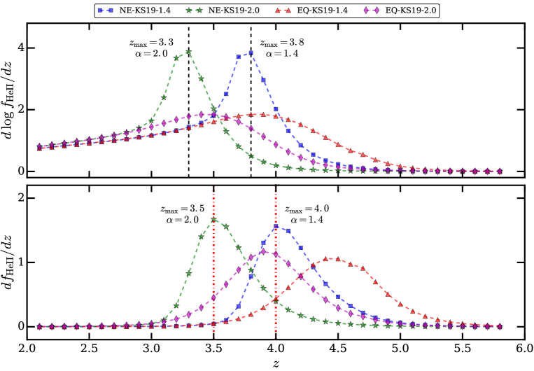
In this section we discuss the evolution of $T_{0}$ and $\gamma$ for different UVB models discussed in §2.3. Fig. 4 shows the evolution of $T_{0}$ (upper panel) and $\gamma$ (lower panel) for KS19 UVB obtained using quasar SEDs with different values of $\alpha$ (i.e $\alpha=1.4$ and $2.0$). For each UVB model, we show the $T_{0}$ and $\gamma$ evolution for equilibrium and non-equilibrium cases. We now focus on the results for $\alpha=1.4$ i.e., models EQ-KS19-1.4 and NE-KS19-1.4 (the results are qualitatively similar for $\alpha=2.0$ models as well). As expected based on P15 find that $T_{0}$ in the non-equilibrium model is higher as compared to that from the equilibrium model at any given epoch for $z<4.5$. As we discussed earlier,  $f_{\rm HeII}$ is larger in the non-equilibrium model as compared to that in equilibrium at $3.5<z<5$. As a result photo-heating (and hence temperature), which is proportional to  $f_{\rm HeII}$ (see Eq. 2.1), is more in the non-equilibrium model. The maximum obtained temperature for the non-equilibrium model ($\sim 14500$ K) is substantially higher as compared to that of equilibrium model ($\sim 10000$ K) at $3.5<z<5$. Even though  $f_{\rm HeII}$ for the non-equilibrium model is smaller than that for equilibrium model at $z<3.5$ (see Fig. 2), it takes a long time (time scale $\sim$ Hubble time) for the gas to cool and reach equilibrium. We also see more flattening (smaller $\gamma$) of the TDR in non-equilibrium model as compared to equilibrium model. This is because the  $f_{\rm HeII}$ (and hence photo-heating Eq. 2.1) in the non-equilibrium model is independent of density (see Appendix B).

We next use the same figure to compare the $T_{0}$ and $\gamma$ evolution in the non-equilibrium models for the two values of $\alpha$ (1.4 and 2.0) i.e., models NE-KS19-1.4 and NE-KS19-2.0. The maximum $T_{0}$ obtained in NE-KS19-1.4 ($T_{0}\sim 14500$ K at $z=3.7$) is higher by 17 percent than that from NE-KS19-2.0 ($T_{0}\sim 12000$ K at $z=3.3$). This is expected as a higher value of $\alpha$ corresponds to less kinetic energy per photo-electron at $\lambda<228{\rm\AA}$. This excess energy would be less for the case of $\alpha=2.0$ as compared to $\alpha=1.4$. The trend in $T_{0}$ vs $z$ seen in this figure can explain the kink we noticed in Fig. 2 for $\alpha=1.4$ model.

The peak in $T_{0}$ evolution for non-equilibrium model occurs at lower redshift for higher $\alpha$ ($z=3.3$ for $\alpha=2.0$ and $z=3.7$ for $\alpha=1.4$). This is consistent with the redshift evolution of  $f_{\rm HeII}$ where we show that the redshift of reionization is lower for higher value of $\alpha$ (see §3.1.1). It is interesting to note that for the non-equilibrium models, peak in $T_{0}$ evolution occurs at redshift where $f_{\rm HeII}\sim 0.055$ whereas the valley in $\gamma$ occurs at redshift where $f_{\rm HeII}\sim 0.25$ irrespective of UVB. This also implies that the peak in the $T_{0}$ evolution and valley in the $\gamma$ evolution do not necessarily occur at the same redshift. This behaviour of $T_{0}$ and $\gamma$ is correlated with the time-derivative of  $f_{\rm HeII}$. We show the derivative of $\log f_{\rm HeII}$ (top panel) and  $f_{\rm HeII}$ (bottom panel) with respect to $z$ in Fig. 5. One can see that the peak in $d\log f_{\rm HeII}/dz$ is nicely correlated with the peak in $T_{0}$ whereas the epoch of the minimum $\gamma$ is correlated with $df_{\rm HeII}/dz$. The above trend is also seen in the case of equilibrium models. However peak in $T_{0}$ and $\gamma$ for equilibrium models are quite broad.

3.2 Evolution of the effective optical depth

Figure 6: $\Gamma_{\rm 12}$ constraints from equilibrium (left panel) and non equilibrium models (right panel) using $\tau_{\rm eff,HI}$ along with the measurements from Becker & Bolton (2013). The observed $\tau_{\rm eff,HI}$ from Faucher-Giguère et al. (2008a, black stars), Becker & Bolton (2013, blue squares with errorbars) and Becker et al. (2015, orange triangles) are shown in left and middle panel. Left panel shows the $\tau_{\rm eff,HI}$ evolution from equilibrium models for $\alpha=1.4$ (black solid line) and $\alpha=2.0$ (blue solid lines) in KS19 UVB model. The red shaded region shows the uncertainty in $\tau_{\rm eff,HI}$ due to uncertainty in $\alpha$ for equilibrium models. $\tau_{\rm eff,HI}$ evolution for $1.4<\alpha<2.0$ lies within red shaded region. Middle panel is similar to left panel except that the $\tau_{\rm eff,HI}$ evolution is shown for non-equilibrium models. The green shaded region shows the uncertainty in $\tau_{\rm eff,HI}$ due to uncertainty in $\alpha$ ($1.4\leq\alpha\leq 2.0$) for non-equilibrium models. The $\tau_{\rm eff,HI}$ evolution matches well for the KS19 non-equilibrium UVB model than that for KS19 equilibrium UVB model. In both panels, we also show the $\tau_{\rm eff,HI}$ evolution for equilibrium and non-equilibrium model using HM12 UVB. Right panel shows the comparison of $\tau_{\rm eff,HI}$ evolution for equilibrium and non-equilibrium models. The kink in the  $f_{\rm HI}$ distribution in Fig. 2 for NE-KS19-1.4 (red dotted line) manifest itself as a broad dip in the $\tau_{\rm eff,HI}$ at $z\sim 3.8$.

Figure 7: Each panel shows the evolution of median  He ii effective optical depth ($\tau_{\rm eff,HeII}$) from observations (Worseck et al., 2018, red circles with errorbar) and from simulations (blue stars with errorbars). The gray shaded regions correspond to 16^th and 84^th percentile on simulated median $\tau_{\rm eff,HeII}$ (consistent with the corresponding range obtained by Worseck et al., 2018). The median $\tau_{\rm eff,HeII}$ and associated errorbars in simulation are calculated in a way similar to that of Worseck et al. (2018). The $\tau_{\rm eff,HeII}$ from simulation are shifted along $x$ axis by $\Delta z=0.01$ for clarity. The simulated  He ii  Ly$\alpha$ forest mimic the observations by accounting for the effects of exposure time (varying SNR), HST-COS LSF, redshift path length and Poisson noise properties that vary along different quasar sightlines (Table 1 in Worseck et al., 2018). Top (panel a, b, c and d) and bottom (panel e, f, g and h) rows show the median $\tau_{\rm eff,HeII}$ evolution for equilibrium and non-equilibrium models (model name is given in each panel) respectively. The median $\tau_{\rm eff,HeII}$ evolution from model EQ-KS19-1.8 (panel c) and NE-KS19-2.0 (panel h) are in good agreement with that from observations. Interestingly, our models produce the lower limits of $\tau_{\rm eff,HeII}$ at $z>3$ reasonably well whether we consider equilibrium or non-equilibrium evolution. The large $\tau_{\rm eff,HeII}$ scatter in our model at $z>3$ is due to fluctuations in the density field (UVB is assumed to be uniform). The median $\tau_{\rm eff,HeII}$ evolution at $z<2.8$ is sensitive to $\alpha$. The observed $\tau_{\rm eff,HeII}$ evolution from Worseck et al. (2018) is well reproduced by with $\alpha=1.8$ for equilibrium models and $\alpha=2.0$ for non-equilibrium models.

Figure 8: Each panel shows the comparison of cumulative distribution function of $\tau_{\rm eff,HeII}$ from observations (blue curve) with that from model NE-KS19-2.0 (uniform UVB model). The model $\tau_{\rm eff,HeII}$ CDF is obtained from 180 mock samples and these are shown by thin gray curves. Each mock sample is mimicked to match observations in terms of SNR, LSF, number of sightlines and redshift path length. The mean $\tau_{\rm eff,HeII}$ CDF from 180 mock samples these are shown by red dashed curve in each panel. The scatter in $\tau_{\rm eff,HeII}$ is relatively well produced by uniform UVB model at $z<2.74$. However, in high-$z$ bins our models have more low optical depth regions compared to the observations. This lack of good matching between the two CDF may favour additional mechanisms like fluctuations in UVB and/or temperature in addition to what we get from density fluctuations only.

In this section, we present the comparison of our model predictions with the observations of  Ly$\alpha$ forest. To generate the forest, we shoot random sight lines through our simulation box and calculate the overdensity ($\Delta$), peculiar velocity ($v$) and temperature ($T$) along these skewers (Choudhury et al., 2001; Padmanabhan et al., 2015; Gaikwad et al., 2017). Since we calculate the temperature of each particle in the post-processing of gadget-2 using cite, we need to correct for the pressure smoothing effects. We follow the procedure given in G18 to generate the  Ly$\alpha$ forest spectra along these sightlines. In G18, we have shown that our method is accurate within 20 per cent with that from self-consistent gadget-3 simulation. We also account for the line spread function (Gaussian with FWHM $\sim 6$  km s^-1), finite SNR ($\sim 20$) for generating the mock  Ly$\alpha$ forest spectra. In the case of  He ii  Ly$\alpha$ forest we have used the line spread function, signal to noise ratio and pixel sampling as appropriate for the HST-COS spectra.

The effective optical depth, $\tau_{\rm eff}=-\log\langle e^{-\tau}\rangle$, where the angle brackets indicate averaging, is a robust quantity that can be easily derived from observations and simulations for both  H i and  He ii. Fig. 6 shows the evolution of  H i effective optical depth ($\tau_{\rm eff,HI}$) with redshift for different UVB models. The observed $\tau_{\rm eff,HI}$ data points from Faucher-Giguère et al. (2008a); Becker & Bolton (2013); Becker et al. (2015) are also shown in the figure. To calculate $\tau_{\rm eff,HI}$ from simulations, we use boxes at $z=2.1$ to $5.0$ with $\Delta z=0.1$. For each UVB model, we calculate $\tau_{\rm eff,HI}$ using 500 sight lines at each redshift.

The left panel of Fig. 6 shows the results for the equilibrium models for KS19 UVB and HM12. We can see that the $\tau_{\rm eff,HI}$ is consistently larger for $\alpha=2.0$ as compared to that for $\alpha=1.4$. This is expected as $\tau_{\rm eff}\propto T_{0}^{-0.7}$ because of the temperature dependence of the recombination rate coefficient and $T_{0}$ is consistently larger for smaller $\alpha$ (as we have already seen in Fig. 4). We show the $\tau_{\rm eff,HI}$ for $1.4<\alpha<2.0$ as the red shaded region with the upper and lower envelops of this shaded region correspond to $\alpha=2.0$ and 1.4 cases respectively. Interestingly, $\tau_{\rm eff,HI}$ for the KS19 and HM12 equilibrium models are consistently higher than those from observations at $z<4$, with the mismatch being maximum at the lowest redshifts. Thus for our simulations, to match the observed $\tau_{\rm eff,HI}$, we would require $\Gamma_{\rm HI}$ which is 18 percent lower than values obtained for KS19.

The middle panel in Fig. 6 is similar to the left one except that the $\tau_{\rm eff,HI}$ evolution is shown for non-equilibrium UVB models for KS19 and HM12. Since $T_{0}$ is consistently higher for the non-equilibrium models as compared to the equilibrium models, $\tau_{\rm eff,HI}$ for the non-equilibrium model is lower. Interestingly, this makes the $\tau_{\rm eff,HI}$ evolution for non-equilibrium case match better with the observations in the range from $z=5$ to $z=2.5$. This also implies that, for a given set of cosmological parameters, the observed $\tau_{\rm eff,HI}$ would lead to different $\Gamma_{\rm HI}$ depending on whether one uses the equilibrium or the non-equilibrium model while comparing with the data. The kink we noticed in the predicted  $f_{\rm HI}$ distribution in Fig. 2 for NE-KS19-1.4 manifest itself as a broad dip in the $\tau_{\rm eff,HI}$ curve as evident in the lower envelop at $z\sim 3.8$ (right panel in Fig. 6). Similar broad dip in $\tau_{\rm eff,HI}$ is also seen in P15 for HM12 UVB.

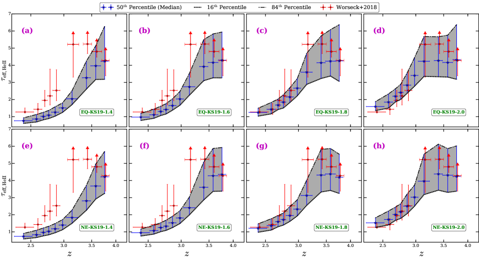
Moving on to  He ii, we show the evolution of $\tau_{\rm eff,HeII}$ with redshift for different UVB models for equilibrium and non-equilibrium considerations in Fig. 7. For comparison, we use the observed median, 16^th and 84^th percentile of $\tau_{\rm eff,HeII}$ over different redshift bins listed in table 4 of Worseck et al. (2018). These were obtained with quasar spectra observed with different spectral resolution (i.e line spread functions, LSFs) and exposure times (i.e varied SNR). In order to make realistic comparisons, while computing the distribution of $\tau_{\rm eff,HeII}$ from our simulations we used appropriate combinations of LSF and SNR. Inferred flux or optical depth at the bottom of the saturated lines will be dominated by photon noise originating from the background subtraction. We also model this effect carefully.

The shaded regions in Fig 7 are our model predicted regions covering 16^th and 84^th percentile of $\tau_{\rm eff,HeII}$. When we consider the equilibrium models (i.e upper panels in Fig. 7), the UVB computed using $\alpha=1.8$ (panel c) reproduces the observed median and the scatter very well for $z<2.8$. This model also captures the flattening of $\tau_{\rm eff,HeII}$ with large scatter seen in observations at high-$z$ very well. From the figure 3 of Worseck et al. (2018) we can see that the equilibrium simulations using uniform UVB of Puchwein et al. (2019) produce much sharper evolution of $\tau_{\rm eff,HeII}$ as a function of $z$ compare to our models. This is probably related to sharper increase in $\Gamma_{\rm HeII}$ produced by the UVB of Puchwein et al. (2019) compared to those used in our models. It is also clear that the scatter we find in $\tau_{\rm eff,HeII}$ is much more than what has been found for constant $\Gamma_{\rm HeII}$ models considered by Worseck et al. (2018). Thus our models seem to produce a reasonable agreement to the data unlike the uniform background models considered in Worseck et al. (2018). This is not surprising as constraints from He ii measurements were used while constructing the UVB used in our study (see Khaire, 2017). From Fig 7 we notice that at $z>3$, 16^th percentile $\tau_{\rm eff,HeII}$ from our models may be lower than what is observed (even when we match the limiting values in two redshift bins observational limits are higher in the middle two $z$ bins).

Next we consider the non-equilibrium models (lower panels in Fig. 7). As expected $\tau_{\rm eff,HeII}$ obtained at $z<2.8$ are lower than that obtained for the corresponding equilibrium cases. Thus in order to match the observed data we require UVB obtained with slightly larger value of $\alpha$ (i.e $\alpha=2$, panel h). On the other hand non-equilibrium models provide slightly higher values of $\tau_{\rm eff,HeII}$ at $z>3$ compared to the corresponding equilibrium models. However even in this case observed limits in two redshift bins are higher than that predicted by our models.

In summary, both equilibrium and non-equilibrium models reproduce the observed trend of $\tau_{\rm eff,HeII}$ as a function of $z$. As we use uniform UVB, the large $\tau_{\rm eff,HeII}$ scatter produced by our models at $z>3$ is mainly due to fluctuations in the density field and evolution in $\Gamma_{\rm HeII}$ (also see Appendix C). For the constant $\Gamma_{\rm HeII}$ value used by Worseck et al. (2018), we expect $\tau_{\rm eff,HeII}$ scatter to be smaller than what is produced by our models. The UVB used by Puchwein et al. (2019) produces larger $\tau_{\rm eff,HeII}$ than what is observed while producing large scatter. It is important to note that the effect of simulation box size, mass resolution (Bolton et al., 2017), finite noise, spectral resolution and redshift path length in the observed spectra have weaker effect on $\tau_{\rm eff,HeII}$ scatter at $z>3$. Our study shows the observed range of $\tau_{\rm eff,HeII}$ at $z<2.8$ can be used to place constraints on the quasar spectral index $\alpha$ (also see Khaire, 2017). The non-equilibrium models require higher value of $\alpha$ compared to the equilibrium models. Our models produce the enhanced scatter in $\tau_{\rm eff,HeII}$ at $z>3$ with non-equilibrium models producing slightly higher values. However, if the observed $\tau_{\rm eff,HeII}$ at $z>3$ are not dominated by small number statistics then our model predicted 16^th quartile values (both equilibrium and non-equilibrium case) may be smaller than what has been observed. We show the comparison of mean $\tau_{\rm eff,HeII}$ evolution from our models with that from observations (Heap et al., 2000; Zheng et al., 2004; Fechner et al., 2006; Syphers & Shull, 2014; Worseck et al., 2016) in Appendix D (see Fig. 13). Qualitatively our mean $\tau_{\rm eff,HeII}$ evolution is consistent with that from Puchwein et al. (2015, 2019).

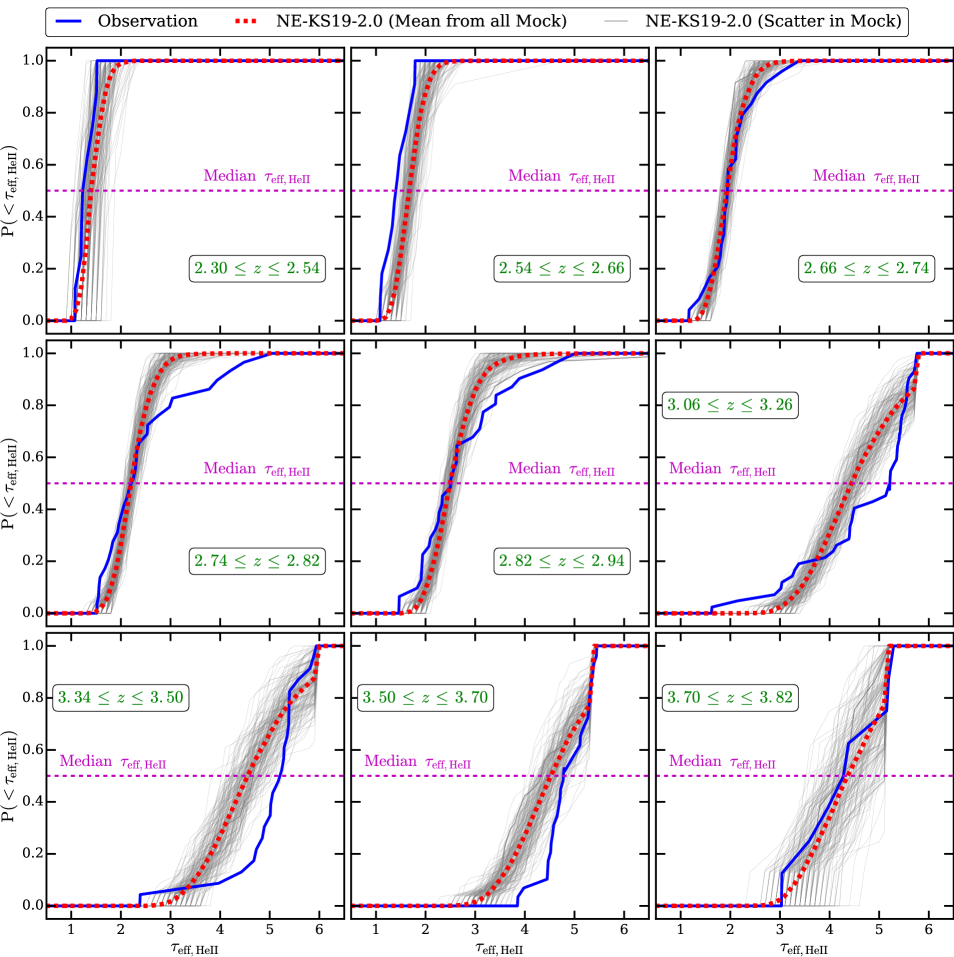
Fig. 8 shows the comparison of cumulative distribution function (CDF) of $\tau_{\rm eff,HeII}$ from observations with that from model NE-KS19-2.0 (uniform UVB model) at $2.30\leq z\leq 3.82$. We show $\tau_{\rm eff,HeII}$ CDF for NE-KS19-2.0 model since the median $\tau_{\rm eff,HeII}$ evolution from this model is in good agreement with observations (Fig. 7). The model $\tau_{\rm eff,HeII}$ CDF in Fig. 8 is obtained from 180 mock samples. Each mock sample is mimicked to match observations in terms of SNR, LSF, number of sightlines and redshift path length. The scatter in $\tau_{\rm eff,HeII}$ is relatively well produced by uniform UVB model at $z<2.74$. However, the $\tau_{\rm eff,HeII}$ scatter from uniform UVB model is smaller than the observed CDF for higher redshift bins. Thus, while we could produce larger scatter in median $\tau_{\rm eff,HeII}$ covering the observed scatter using an uniform UVB, the analysis presented here suggests that we may need additional sources of scatter like fluctuations in the UVB and/or temperature to explain the observed CDF. As mentioned before consideration of non-equilibrium evolution does not produce significantly large scatter than the equilibrium models.

As discussed above our models require small fine-tuning of the ionizing background (mainly the normalization) to match the $\tau_{\rm eff,HI}$ as a function of $z$. For example, one may have to increase the value of $\Gamma_{\rm HI}$ (by $\sim 18$ percent) which may result in the reduction of $\Gamma_{\rm HeII}$ through radiative transport effects as shown in Khaire & Srianand (2013). This will in turn increase the $\tau_{\rm eff,HeII}$. We plan to carry out such a self-consistent modelling in near future. Note Worseck et al. (2018) explained the observed $\tau_{\rm eff,HeII}$ as a function of $z$ using fluctuating UVB models. Moreover, the fluctuations in the temperature due to residual heating from  He ii reionization could be important in the redshift of interest (Keating et al., 2018). Given that the simulation box size used in our study is small, modelling the effect of fluctuating UVB and temperature will not be possible in the present case. However, our study emphasizes the non-equilibrium effects that will be important even when one uses fluctuating UVB and temperature. We would like to emphasize here that even for models that includes fluctuating UVB, our post-processing code will be handy in incorporating non-equilibrium effects.

3.3 $\Gamma_{\rm HI}$ constraints

Figure 9: Each panel shows constraint on $\Gamma_{\rm 12}$ from this work. The $\Gamma_{\rm 12}$ constraints from Becker & Bolton (2013) are shown for $\gamma=1.2,1.4$ and $1.6$ by green, blue and orange solid lines respectively. Left panel shows $\Gamma_{\rm 12}$ constraints for $\alpha=1.4$ (red stars) and $\alpha=2.0$ (magenta squares) KS19 equilibrium UVB model. The red shaded region shows the uncertainty in $\Gamma_{\rm 12}$ due to uncertainty in $\alpha$ ($1.4\leq\alpha\leq 2.0$). Right panel is similar to left panel except the $\Gamma_{\rm 12}$ constraints are shown for non-equilibrium model. The green shaded region encompasses allowed $\Gamma_{\rm 12}$ for $\alpha$ in the range $1.4\leq\alpha\leq 2.0$. The redshift evolution of $\Gamma_{\rm 12}$ constraints is different in equilibrium and non-equilibrium models.

One or more of observed $\tau_{\rm eff,HI}$, flux probability distribution function or flux power spectrum of  Ly$\alpha$ absorption are used to constrain $\Gamma_{\rm HI}$ (Bolton & Haehnelt, 2007; Faucher-Giguère et al., 2008c; Becker & Bolton, 2013; Gaikwad et al., 2017). However for a given density field the above mentioned quantities also depend on the gas temperature and thermal history through pressure smoothing (Gnedin & Hui, 1998; Kulkarni et al., 2015). Thus it is a usual procedure to use simulations with varied thermal histories to measure $\Gamma_{\rm HI}$ as a function of $z$ (Becker et al., 2011; Becker & Bolton, 2013). Here we ask how the inferred $\Gamma_{\rm HI}$ for a given observed $\tau_{\rm eff,HI}$ depends on whether one uses equilibrium or non-equilibrium evolutions.

Typical steps followed in constraining $\Gamma_{\rm HI}$ involves,

1. generating  Ly$\alpha$ forest in simulation for a given UVB (and hence ionization and thermal history) using either equilibrium or non-equilibrium conditions,

2. compare the observed $\tau_{\rm eff,HI}$ with predictions from the simulation,

3. rescaling the simulated $\Gamma_{\rm HI}$ at a given epoch in the post-processing step to make the $\tau_{\rm eff,HI}$ from simulations match with that from observations and

4. repeating the step (i) to (iii) for different UVB.

Note that we have implicitly assumed here that changing the value of $\Gamma_{\rm HI}$ locally does not affect the thermal history at redshifts of our interest. Also at the redshift of our interest collisional ionization is sub-dominant. This is a reasonable approximation if the applied scaling is at the level of few percent. The first step in obtaining different thermal histories is computationally expensive as explained in §2. In our case we use cite to generate the simulations for an assumed UVB.

We use Becker & Bolton (2013, their table 2) $\tau_{\rm eff,HI}$ measurements to constrain $\Gamma_{\rm HI}$ in 7 redshift bins centred at $z=2.4-4.8$ with $\Delta z=0.4$. Becker & Bolton (2013) have tabulated the $\tau_{\rm eff,HI}$ measurements from observations accounting for the possible systematics such as metal contaminations, continuum placement uncertainty, correction for the presence of optically thick absorbers etc (also see Faucher-Giguère et al., 2008a). For each of our models we constrain $\Gamma_{\rm HI}$ by finding the root ($\Gamma_{\rm HI}$ value) that matches model $\tau_{\rm eff,HI}$ with observed $\tau_{\rm eff,HI}$ at a given redshift. We use scipy’s optimize module to find the root (function tolerance set to $10^{-9}$). We use 2000 sight lines to calculate the $\tau_{\rm eff,HI}$ from simulation at any given redshift. We splice sight lines to match the observed redshift path length ($\Delta z=0.4$). We add a Gaussian random noise of SNR$=20$ to the simulated  Ly$\alpha$ forest spectra.

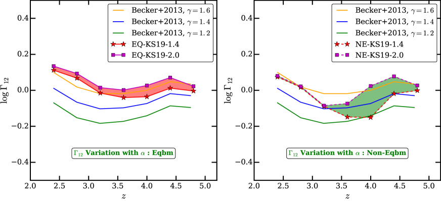
The left and right panels in Fig. 9 show $\Gamma_{\rm 12}$ constraints ($\Gamma_{\rm HI}$ in $10^{-12}\>{\rm s}^{-1}$) for EQ-KS19 and NE-KS19 models respectively from this work. In each panel, we show the $\log\Gamma_{\rm 12}$ for two values of $\alpha=1.4$ and $2.0$. First, we consider the variation in $\log\Gamma_{\rm 12}$ due to variation in $\alpha$ for a given model i.e., either EQ-KS19 or NE-KS19. The best-fit $\log\Gamma_{\rm 12}$ values are systematically higher for smaller values of $\alpha$. This is consistent with the evolution of $T_{0}$ in Fig. 4 where $T_{0}$ is consistently larger for smaller values of $\alpha$ irrespective of whether we use EQ-KS19 or NE-KS19 model. Since for a given $\tau_{\rm eff,HI}$ we have $\Gamma_{\rm HI}\propto T_{0}^{-0.7}$, the constrained $\log\Gamma_{\rm 12}$ values are systematically higher for larger $\alpha$. The same explanation also holds when we compare the $\Gamma_{\rm 12}$ constraints from models with same $\alpha$ but different ionization evolution i.e., EQ-KS19-1.4 (EQ-KS19-2.0) and NE-KS19-1.4 (NE-KS19-2.0) models. Since $T_{0}$ is systematically larger for NE-KS19-1.4 model than in the EQ-KS19-1.4 model, $\log\Gamma_{\rm 12}$ in NE-KS19-1.4 is consistently smaller in EQ-KS19-1.4 model. We also find that the $\Gamma_{\rm HI}$ constraints are relatively insensitive to the choice of initial $T_{0}$, $\gamma$ we use at $z=6$ in cite (see Appendix E for details).

We now consider the allowed range in $\log\Gamma_{\rm 12}$ as shown by red and green shaded regions in the left and right panels of Fig. 9 respectively. We also show $\log\Gamma_{\rm 12}$ measurement from Becker & Bolton (2013) for $\gamma=1.2,1.4$ and $1.6$ in each panel of Fig. 9. The derived $\log\Gamma_{\rm 12}$ range and its redshift dependences for NE-KS19 model (green shaded region in right panel) at $3.5<z<5$ are different compared to those obtained for EQ-KS19 (red shaded region in left panel) models. This is a direct consequence of difference in $T_{0}$ and $\gamma$ evolution between these models. Fig. 9 also shows that the minimum in $\log\Gamma_{\rm 12}$ at $z\sim 3.5$ is more prominent in non-equilibrium models than that in equilibrium models.

The difference in the derived shape of $\Gamma_{12}$, in particular a prominent valley observed at $z\sim 3.5$ can naively imply that there are two kinds of sources, one dominating the UV background at $z<3.5$ and another at $z>3.5$. For example, it will not be straightforward to obtain such a valley-like feature in the UVB models using only one population of sources such as quasars (see for e.g Madau & Haardt, 2015; Khaire et al., 2016). One will be forced to invoke stronger evolution in $f_{\rm esc}$ than the one assumed in these models.

To summarize, the widely used technique to obtain $\Gamma_{\rm HI}$ from observed $\tau_{\rm eff,HI}$ distribution calibrated by simulations can result in $\Gamma_{\rm HI}$ evolution that is very different from the intrinsic distribution depending upon whether one uses equilibrium and non-equilibrium models. In particular in the redshift range where He ii reionization takes place it will be important to simultaneously model $\tau_{\rm eff,HI}$, $\tau_{\rm eff,HeII}$ and $T_{0}$ and $\gamma$ evolutions to place constraints on the nature of UV ionizing background. Becker & Bolton (2013) constrained $\Gamma_{\rm HI}(z)$ using a range of $T_{0}-\gamma$ combinations whose redshift evolution need not be realized in a self-consistent model. Our post-processing code cite allows us to consider self-consistent $T_{0}-\gamma$ for assumed  He ii reionization model under equilibrium and non-equilibrium conditions while constraining $\Gamma_{\rm HI}$. It is clear from the discussions in the previous section that in a physically motivated model the redshift evolution of $T_{0}$ and $\gamma$ can allow us to distinguish between equilibrium and non-equilibrium cases. However, both these quantities are not directly measured but derived from the observed properties of  Ly$\alpha$ forest in the framework of simulations. In the following section we try to see whether one will be able to recover the intrinsic evolution of $T_{0}$ and $\gamma$ using equilibrium models as done in the literature.

3.4 Recovery of $T_{0}$ and $\gamma$ in non-equilibrium recovery from equilibrium model

Figure 10: Panel a shows the wavelet PDF for fiducial model (NE-KS19-1.4, blue circles) and best fit model (EQ-KS19-1.4, red stars). We vary the thermal history in EQ-KS19-1.4 model to obtain the different $T_{0}$ and $\gamma$ combination (see §3.4). The best fit model corresponds to minimum $\chi^{2}$ (or maximum likelihood) between fiducial and model wavelet PDF. The corresponding residuals between fiducial and model wavelet PDF are shown in panel b. Panel c and d are similar to panel a and b respectively except for PDF of curvature statistics. Joint $1\sigma$ contours (maximum likelihood) from wavelet (red solid) and curvature (magenta dashed) statistics are shown in panel e. The marginalized distributions for $T_{0}$ and $\gamma$ are shown for each statistics in panel f and h. Both statistics recover the fiducial (NE-KS19-1.4, shown by green dashed line in panel f and h) $T_{0}$ and $\gamma$ within $1\sigma$ uncertainty. All plots are shown at $z=3.6$ and for KS19-1.4 UVB models.

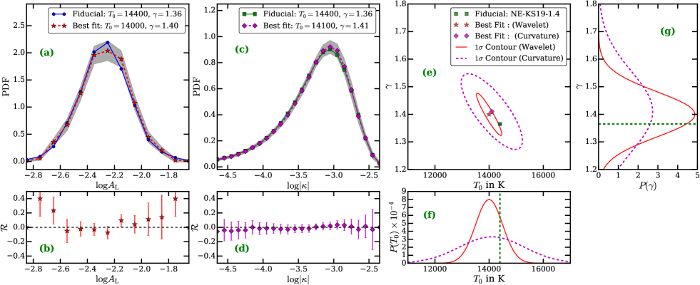
The thermal history of the IGM provides an indirect way of studying  He ii reionization. In the literature, $T_{0}$ and $\gamma$ are constrained from observations by comparing with predictions of simulations having a wide range of thermal histories. However, most of these simulations do not consider non-equilibrium ionization conditions. As shown in §3.1.3, the thermal history of IGM can be considerably different in equilibrium and non-equilibrium ionization models and the non-equilibrium effects could be quite important during  He ii reionization. Hence it is important to investigate whether the thermal history in non-equilibrium models can be recovered using an equilibrium model.

We assume the underlying “true” model to be given by NE-KS19-1.4. We concentrate on $z=3.6$ which is well within period of the  He ii reionization. The thermal parameters at this redshift for the NE-KS19-1.4 are $T_{0}=14400$ K and $\gamma=1.36$. Next, we generate the different thermal histories for the EQ-KS19-1.4 model using the cite. We vary the photo-heating rates as $\epsilon_{\rm X}=a\>\Delta^{b}\>\epsilon_{\rm X,KS19}$ (Becker et al., 2011), where $\epsilon_{\rm X,KS19}$ is photo-heating rate of species ${\rm X}\equiv[{\rm HI,HeI,HeII}]$ in the EQ-KS19-1.4 model (also see Oñorbe et al., 2017, for different approach). A variation in factor $a$ (or $b$) corresponds to change in $T_{0}$ ($\gamma$, respectively) with small variation in $\gamma$ ($T_{0}$, respectively). We varied factor $a$ and $b$ such that the $T_{0}$ varies from 6000 K to 20000 K in steps of 2000 K and $\gamma$ varies from 1.1 to 2.0 in steps of 0.1. In total we generate $8\times 10=80$ different thermal histories from EQ-KS19-1.4 model at $z=3.6$. Note unlike the self-consistent models the pressure smoothing we apply for each particle will depend on its temperature at $z\sim 3.6$ and may not capture the effect of thermal history. However as shown by G18 the effect is of the order of $<20$ percent in the two PDFs discussed here (see section 4.4 and 4.5 in G18)

For each of these simulations (including the underlying “true” model), we shoot $1000$ random sight lines and compute  Ly$\alpha$ forest spectra. We adjust $\Gamma_{\rm HI}$ in all the models such that the mean transmitted flux is same. For fair comparison, we account for the effects of finite SNR and LSF in the  Ly$\alpha$ forest spectra for all the models. In order to constrain $T_{0},\gamma$ from  Ly$\alpha$ forest, we use two statistics namely wavelet statistics (Zaldarriaga, 2002; Theuns et al., 2002; Lidz et al., 2010; Garzilli et al., 2012; Gaikwad et al., 2018) and curvature statistics (Becker et al., 2011; Boera et al., 2014; Padmanabhan et al., 2015; Gaikwad et al., 2018). These statistics have the property that a large value of temperature corresponds to smaller values of curvature and wavelet amplitudes. The method to calculate these statistics is identical to that of G18. We compute $\chi^{2}$ (and maximum likelihood $\mathcal{L}\propto e^{-\chi^{2}/2}$) between the assumed “true” non-equilibrium model and the equilibrium model (for each thermal history) for both the statistics. The best-fit model corresponds to a minimum value of $\chi^{2}$ (or a maximum value of $\mathcal{L}$). The statistical uncertainty in $T_{0}$ and $\gamma$ corresponds to $\chi^{2}=\chi^{2}_{\rm min}+\Delta\chi^{2}$ where $\Delta\chi^{2}=2.30$ for $2$ ($T_{0}$ and $\gamma$ being free parameters) degrees of freedom (Avni, 1976; Press et al., 1992).

Fig. 10 shows the recovery of the “true” (NE-KS19-1.4) $T_{0}$ and $\gamma$ using EQ-KS19-1.4 models with different thermal histories. Panels a and c show the PDFs of the wavelet and curvature statistics respectively for the “true” and best-fit models. The corresponding residuals between the “true” and best-fit models are shown in panels b and d. The reduced $\chi^{2}$ between the “true” and best-fit models for wavelet and curvature statistics are $1.61$ and $1.19$ respectively. Panel e shows the joint $1\sigma$ constrain on $T_{0}-\gamma$ from curvature (magenta dashed curve) and wavelet PDF (red solid curve). The assumed “true” $T_{0}$ and $\gamma$ lie within $1\sigma$ contours for both the statistics. The marginalized distributions (panel f and h) too show that the equilibrium models can recover the non-equilibrium $T_{0},\gamma$ within $1\sigma$ statistical uncertainty. The $T_{0}-\gamma$ constraints from wavelet statistics are better than the curvature statistics because we do not smooth the wavelet amplitude i.e., we use the Eq. 2 to Eq. 6 from Lidz et al. (2010) but we do not use Eq. 7 of Lidz et al. (2010).

In a realistic scenario, one would expect the $T_{0}$ and $\gamma$ evolution to be given by the non-equilibrium models, and hence one should use non-equilibrium simulations to constrain the thermal parameters. Unfortunately, the non-equilibrium models are computationally more expensive than the corresponding equilibrium models, hence exploring a large $T_{0}-\gamma$ parameter space is often impractical with non-equilibrium models. The above result indicates that the underlying non-equilibrium thermal parameters can be recovered by varying the thermal history in equilibrium models, as long as the $\tau_{\rm eff,HI}$ in these models are the same. We also show the effect of matching $\tau_{\rm eff,HI}$ on FPDF and FPS statistics of  H i  Ly$\alpha$ forest in Appendix F. In the literature the $T_{0}$ and $\gamma$ are constrained by allowing the mean flux to vary (see Becker et al., 2011). If this is true at all $z$ then the derived $T_{0}$ and $\gamma$ evolution will reflect whether the underlying evolution is equilibrium or non-equilibrium case.

We caution the reader that our conclusions are based on our model where the large scale fluctuation in $\Gamma_{\rm HeII}$, $T_{0}$ and $\gamma$ expected for fluctuating UVB are not be modelled accurately as the box size (10 $h^{-1}{\rm\,cMpc}$) used is small. Also subtle variations in the pressure smoothing due to small changes in the thermal history are not captured in CITE. A self-consistent radiative transfer simulation with large box size, sufficient mass resolution and non-equilibrium ionization solver is needed to capture these effects (Aubert & Teyssier, 2008; Rosdahl et al., 2013; Gnedin, 2014; Kulkarni et al., 2018). However these simulations may not be flexible enough to probe large parameter spaces.

4 Summary

The cosmological hydrodynamical simulations used to study the properties of  Ly$\alpha$ forest in the literature implement the equilibrium ionization evolution for a given UVB model. However, as we have shown here the assumption of photo-ionization equilibrium may not be valid at $2\leq z\leq 4$ where  He ii reionization is in progress. In addition, the quasar spectral shapes in extreme UV used in the modelling of UVB are observationally ill-constrained. All this can lead to systematics in the derived quantities such as thermal state of the IGM quantified by $T_{0}$ and $\gamma$,  He ii fraction ( $f_{\rm HeII}$),  H i fraction ( $f_{\rm HI}$) and  H i photo-ionization rate ($\Gamma_{\rm HI}$) that are related to  He ii reionization process. In this work, we implement the non-equilibrium ionization evolution in our post-processing tool “Code for Ionization and Temperature Evolution” (cite). Since cite is post-processing module that works on output of gadget-2 (SPH) simulation, we can efficiently simulate the effect of wide range in UVB for equilibrium and non-equilibrium models. We show the consistency of equilibrium and non-equilibrium ionization evolution obtained using cite with those from self-consistent gadget-3 simulations (Puchwein et al., 2015; Gaikwad et al., 2018). Having established this, we explore the effect of unknown quasar UV spectral index on the derived properties of  He ii and  H i absorption as a function of redshift. We summarize our findings as follows,

For a given ionization scenario (equilibrium or non-equilibrium),  $f_{\rm HeII}$ is systematically smaller for UVB models obtained using flatter quasar SEDs at $2\leq z\leq 6$. This suggests that the redshift of  He ii reionization ($z_{\rm reion}$) strongly depends on quasar spectral indices used in the UVB models such that  He ii reionization is earlier ($z_{\rm reion}$ is larger) when flatter quasar SEDs are used. The extent of  He ii reionization ($\Delta z$) is smaller for non-equilibrium models than that from equilibrium models. $\Delta z$ is relatively insensitive to variation in quasar spectral indices.

The globally volume averaged  He ii fraction ( $f_{\rm HeII}$) in non-equilibrium model evolves rapidly from $1$ to $\sim 10^{-2}$ over a small redshift interval $\Delta z=0.85$. Whereas the corresponding change in  $f_{\rm HeII}$ for equilibrium model occurs over a larger redshift interval $\Delta z=1.3$ (see Fig. 2).

For a given UVB, $T_{0}$ in non-equilibrium model is consistently larger than that in equilibrium model at $2\leq z\leq 6$. Whereas in the same redshift range, $\gamma$ is consistently smaller in non-equilibrium model than that in equilibrium model (Puchwein et al., 2015). In all models, we notice that the epoch of minimum $\gamma$ occurs earlier than the epoch of maximum $T_{0}$. The epochs of maximum $T_{0}$ and minimum $\gamma$ are well correlated with derivatives of  $f_{\rm HeII}$ with respect to redshift (see Fig. 5). On the other hand, for a given ionization evolution, $T_{0}$ is consistently larger for models using UVB obtained with flatter quasar spectral index. The epoch of maximum $T_{0}$ (and minimum $\gamma$) is earlier for simulations using UVB compiled with flatter quasar SEDs (Fig. 4). This evolution of $T_{0}$ and $\gamma$ for all models (equilibrium, non-equilibrium and different quasar spectral indices) is consistent with the evolution of  $f_{\rm HeII}$.

For a given set of cosmological parameters and given $\Gamma_{\rm HI}$, we find that the $\tau_{\rm eff,HI}$ at any $z$ is consistently smaller in non-equilibrium model as compared to equilibrium model (Fig. 6). The predicted $\tau_{\rm eff,HI}$ at any $z$ is systematically smaller for models using UVB generated with flatter quasar SED. This is because $T_{0}$ is larger in non-equilibrium and/or for UVB generated with flatter quasar SEDs.

We show the observed median $\tau_{\rm eff,HeII}$ and 16^th and 84^th percentiles regions are well reproduced by both equilibrium and non-equilibrium models. In particular we find that the observed $\tau_{\rm eff,HeII}$ at $z<2.8$ can be used to constrain $\alpha$ values. The equilibrium models require slightly smaller values of $\alpha$ to reproduce the observed range. While our models produce 16^th, 50^th and $84^{th}$ percentile of $\tau_{\rm eff,HeII}$ relatively well with observations, to understand the scatter in $\tau_{\rm eff,HeII}$ we show comparison of observed CDF with model CDF. The scatter in $\tau_{\rm eff,HeII}$ is relatively well produced by uniform UVB models at $z<2.74$. However, the observed $\tau_{\rm eff,HeII}$ scatter at higher redshift is larger than those in uniform UVB models. Thus, this work suggests that we may need additional sources of scatter in $\tau_{\rm eff,HeII}$ such as fluctuations in UVB and /or temperature to explain the observed $\tau_{\rm eff,HeII}$ CDF.

We estimate the $\Gamma_{\rm HI}$ in equilibrium and non-equilibrium models with UVB obtained using quasar spectral indices $\alpha=1.4$ and $2.0$ and by matching the $\tau_{\rm eff,HI}$ from our models with that from Becker & Bolton (2013) observed data. The $\Gamma_{\rm HI}$ estimates are systematically larger for UVB models with higher quasar spectral index at $2.4\leq z\leq 4.8$ due to dependence of $T_{0}$ evolution on quasar spectral index. We find that for a given set of model parameter and a physically motivate $T_{0}-\gamma$ evolution, the redshift dependence of $\Gamma_{\rm HI}$ have different shapes for non-equilibrium and equilibrium models. This exercise demonstrates the need for accurate determination of thermal history parameters in order to measure $\Gamma_{\rm HI}(z)$ accurately (also see Becker & Bolton, 2013). Measuring $\Gamma_{\rm HI}$ accurately is needed to build the physical models of ionizing sources and UVB.

The non-equilibrium models are computationally more expensive than the corresponding equilibrium models. While constraining $T_{0}$ and $\gamma$ from observations, one needs to probe a wide range of UVB. This is usually done by rescaling the photo-heating rates (Becker et al., 2011; Walther et al., 2019) and solving equilibrium ionization evolution. We show that one can recover the physically motivated $T_{0}$ and $\gamma$ in non-equilibrium model from the equilibrium models generated by rescaling photo-heating rates (Fig. 10). Thus one can use equilibrium thermal history models to constrain $T_{0}$ and $\gamma$ from observations provided the $\tau_{\rm eff,HI}$ in these models match with that from observations and differential pressure smoothing effects are negligible.

Appendix A Details of additional simulations

In this section we discuss the details of the additional models analysed in this work. We run a low resolution simulation with $L=10\>h^{-1}\>{\rm\,cMpc}$ and $N^{3}_{\rm particle}=128^{3}$ to study the effect of  H i reionization on $T_{0}$ and $\gamma$ at $z=6$. The models presented in §2 starts from $z=6$ with assumed $T_{0}$ and $\gamma$. In addition, we have developed a semi-numerical method to efficiently compute the thermal history for the given UVB from high redshift $z=15$ with better time resolution. Such semi-numerical method also provides the insight in to the non-equilibrium effects on TDR. Furthermore, it is important to check the consistency of our method with self-consistent gadget-3 simulation. For this purpose, we use self-consistent equilibrium and non-equilibrium gadget-3 simulation from P15. The additional models analysed in this work are summarized in Table 3. In order to distinguish various simulations for different UVB model, we use following nomenclature. Model L10-N512-G2-EQ-KS19-2.0 refers to $L_{\rm box}=10h^{-1}\>$  cMpc, $N_{\rm particle}=512$, gadget-2 simulation post-processed with cite for equilibrium ionization evolution using KS19 UVB with SED $\alpha=1.4$. Model L20-N512-G3-NE-HM12-P15 corresponds to $L_{\rm box}=20h^{-1}\>$  cMpc, $N_{\rm particle}=512$, gadget-3 simulation for self-consistent non-equilibrium ionization evolution using HM12 UVB from P15 paper.

Table 3: Nomenclature of the models analyse in this work.

Model Name	$L_{\rm box}$a	$N_{\rm particle}$a	$m_{\rm gas}$a	Codeb	Ionization evolution	UVB	Output Redshift	Reference
L10-N512-G2-EQ-HM12	10	512	$10^{5}$	gadget-2 + cite	equilibrium	HM12	$z=6-1.6,\Delta z=0.1$	This work
L10-N512-G2-NE-HM12	10	512	$10^{5}$	gadget-2 + cite	Non-equilibrium	HM12	$z=6-1.6,\Delta z=0.1$	This work
L10-N512-G2-EQ-KS19-$\alpha$d	10	512	$10^{5}$	gadget-2 + cite	equilibrium	KS19	$z=6-1.6,\Delta z=0.1$	This work
L10-N512-G2-NE-KS19-$\alpha$d	10	512	$10^{5}$	gadget-2 + cite	Non-equilibrium	KS19	$z=6-1.6,\Delta z=0.1$	This work
L10-N128-G2-EQ-HM12	10	128e	$10^{7}$	gadget-2 + cite	equilibrium	HM12	$z=15-1.6,\Delta z=0.1$	This work
L10-N128-G2-NE-HM12	10	128e	$10^{7}$	gadget-2 + cite	Non-equilibrium	HM12	$z=15-1.6,\Delta z=0.1$	This work
L10-N128-G2-EQ-KS19-$\alpha$d	10	128e	$10^{7}$	gadget-2 + cite	equilibrium	KS19	$z=15-1.6,\Delta z=0.1$	This work
L10-N128-G2-NE-KS19-$\alpha$d	10	128e	$10^{7}$	gadget-2 + cite	Non-equilibrium	KS19	$z=15-1.6,\Delta z=0.1$	This work
L20-N512-G3-EQ-HM12-P15c	20	512	$10^{6}$	gadget-3	equilibrium	HM12	$z=6-1.6,\Delta z=0.1$	P15
L20-N512-G3-NE-HM12-P15	20	512	$10^{6}$	gadget-3	Non-equilibrium	HM12	$z=6-1.6,\Delta z=0.1$	P15
SN-EQ-HM12	-	-	-	Semi-Numerical	equilibrium	HM12	$z=15-1.6,\Delta z=0.001$	This work
SN-NE-HM12	-	-	-	Semi-Numerical	Non-equilibrium	HM12	$z=15-1.6,\Delta z=0.001$	This work

• $L_{\rm box}$, $N^{3}_{\rm particle}$ and $m_{\rm gas}$ is length (in $h^{-1}$  cMpc), number of particles and gas mass resolution (in $\rm M_{\odot}$) in simulation box respectively.

• Post-processing module cite is applied on gadget-2 output. cite provides flexibility to change UVB and perform equilibrium / Non-equilibrium ionization evolution efficiently.

• We use P15 simulations to check the consistency of our method.

• SED ($\alpha$) is a free parameter in KS19 UVB. We vary $\alpha$ from 1.4 to 2.0 in steps of 0.1 and solve equilibrium / Non-equilibrium ionization evolution equation. However in this work, we present the results only for $\alpha=1.4,1.6,1.8$ and $2.0$.

• We use low resolution simulation $N_{\rm particle}=128$ to study the thermal history from $z=15$ to $z=1.6$.

Appendix B Semi-numerical model for thermal history

Figure 11: TDR from semi-numerical approximation at $z=3.5$. TDR deviates from power law at $\log\Delta<-1$ for non-equilibrium model (blue stars). TDR in the $\log\Delta$ range -0.5 to 0.5 is fitted with power law and is shown by dashed lines (blue, red line for non-equilibrium, equilibrium models respectively).

Figure 12:  $f_{\rm HeII}$ as a function of $\log\Delta$ for SN-EQ-KS19-14 and SN-NE-KS19-1.4 models at $z=4.0,3.8,3.7$. At all redshifts,  $f_{\rm HeII}$ is proportional to $\Delta^{0.6}$ (Eq. 5) for equilibrium models. Whereas for non-equilibrium  $f_{\rm HeII}$ is independent of $\Delta$ for $\log\Delta<-0.5$ at $z=4.0,3.8$. At $z=3.7$,  $f_{\rm HeII}$ from non-equilibrium model is in good agreement with that from equilibrium model and follows $f_{\rm HeII}\propto\Delta^{0.6}$.

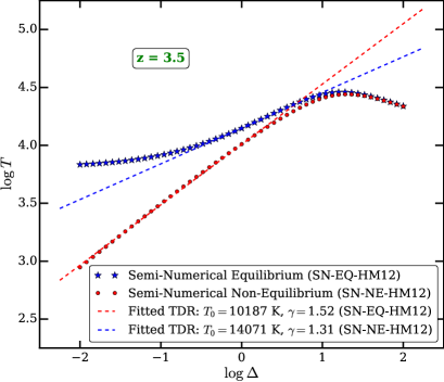
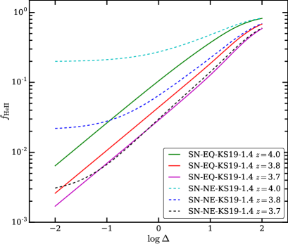
In this section we present a semi-numerical method (refer as SN-EQ-HM12 and SN-NE-HM12 in Table 3) to efficiently predict the evolution of thermal history parameters for a given UVB model. This method is fast and we can quickly check the effect of UVB on thermal history parameters without running full hydro simulation. This is especially helpful in exploring the parameter space for constraining $T_{0}$ and $\gamma$ from observations (see §3.4). In semi-numerical method, we can start from relatively high redshift and evolve the temperature of the IGM with better time resolution. The method is similar to single-cell approximation as described in Puchwein et al. (2019). However, we solve the temperature evolution equation at range of $\Delta$ instead of temperature evolution at $\Delta=1$ (as done in Puchwein et al., 2019). We fit a power-law TDR as explained in §3.1.2. As a result, in addition to $T_{0}$ evolution, we can also predict the evolution in $\gamma$. The main steps involve in the method are as follows,

• First we assume that there are $N=200$ cells with overdensity varying from $\log\Delta=-2.0$ to $2.0$ in steps of $0.02$.

• We assume that the overdensity does not evolve with redshift i.e., $d\Delta/dt=0$ for all cells and there is no heating of the gas due to virial shocks $dT_{\rm shock}/dt=0$.

• Under these assumptions, we solve ionization evolution (equilibrium and/or non-equilibrium) Eq. 2 for each cell and calculate radiative heating and cooling terms ($dQ/dt$ term).

• We then calculate the temperature for each cell from Eq. 1.

Fig. 11 shows the TDR for the cells at $z=3.5$ from equilibrium and non-equilibrium ionization evolution. As expected, the temperature in non-equilibrium case is consistently higher than that from equilibrium case. The TDR is also flattened in non-equilibrium case due to density independent photo-heating of the gas (similar to Fig. 3). The equilibrium and non-equilibrium TDR are fitted with power-law TDR models as shown by dashed lines. One can also see the deviation from power-law at small densities in non-equilibrium models (see Fig. 3). This deviation in TDR for non-equilibrium model occurs at low densities because  $f_{\rm HeII}$ at these densities is independent of density.

Fig. 12 shows  $f_{\rm HeII}$ as a function of $\log\Delta$ for SN-EQ-KS19-1.4 and SN-NE-KS19-1.4 models at $z=4.0,3.8$ and $3.7$. This choice of redshift is motivated by the fact that $\gamma$ is smallest at $z=4.0$, $T_{0}$ is highest at $z=3.8$ and  He ii reionization is completed at $z=3.7$ for KS19-1.4 models (see Fig. 4 and Table 2 for our definition).

First we see a well defined power-law relation between  $f_{\rm HeII}$ and $\Delta$ for equilibrium models at all $z$. This is because  $f_{\rm HeII}$ for photo-ionization equilibrium is given by,

$$f_{\rm HeII} =\frac{n_{\rm HeII}}{n_{\rm He}}=\frac{n_{\rm e}\>n_{\rm HeIII}\>\alpha_{\rm HeIII}(T)}{\Gamma_{\rm HeII}\>n_{\rm He}}$$ (5)

$$f_{\rm HeII} \propto\Delta\>T^{-0.7}$$

$$f_{\rm HeII} \propto\Delta^{1-0.7(\gamma-1)}$$

$$f_{\rm HeII} \propto\Delta^{0.6}$$

where in the last expression we assume, $\gamma\sim 1.57$ (see Fig. 4) for equilibrium case. One can see from Fig. 12 that the  $f_{\rm HeII}$ and $\Delta$ are well related by power law for equilibrium case. The power-law fit to  $f_{\rm HeII}$ vs $\Delta$ curve yields the slope of $\sim 0.61$ for the equilibrium case. Thus one expects to see the power-law relation between  $f_{\rm HeII}$ and $\Delta$ for equilibrium case.

On the other hand,  $f_{\rm HeII}$ at $\log\Delta<0.5$ is flatter (i.e., independent of $\log\Delta$) for SN-NE-KS19-1.4 models at $z=4.0$ and $z=3.8$. The volume averaged  $f_{\rm HeII}$ in L10-N512 simulation at $z=4.0,3.8$ is 0.25, 0.055 (for KS19-1.4 non-equilibrium models) respectively. Thus at these redshifts the  He ii reionization is still not completed. As given in Table 2, the  He ii reionization in non-equilibrium case is completed around $z=3.7$ (for KS19-1.4 non-equilibrium model). At $z=3.7$, we see a good match between  $f_{\rm HeII}$ for equilibrium and non-equilibrium model in Fig. 12. Note that $z=3.7$ is also the redshift at which photo-ionization equilibrium is achieved in SN-NE-KS19-1.4 model.

There is no scatter in our TDR for semi-numerical method since we have neglected the $d\Delta/dt$ and $dT_{\rm shock}/dt$ term in Eq. 1. Thus evolution of density and shock heating of gas is reflected as the scatter in TDR (see Fig. 3).

Fig. 14 shows the comparison of the $T_{0}$, $\gamma$ evolution from the semi-numerical method with L10-N512-G2 and L10-N128-G2 simulations for HM12 UVB model. The differences in $T_{0}$ and $\gamma$ are less than 11 percent for semi-numerical method.

Appendix C Scatter in  He ii effective optical depth

In this section, we show the dependence of $\tau_{\rm eff,HeII}$ scatter on various thermal and ionization parameters of IGM. Assuming fluctuating Gunn-Peterson relation for  He ii (where $K$ is constant that depends on cosmology.),

$$\tau_{\rm HeII} =K\>\frac{T_{0}^{-0.7}\>\Delta^{2-0.7(\gamma-1)}}{\Gamma_{\rm HeII}}$$ (6)

$$\frac{\delta\tau_{\rm HeII}}{\tau_{\rm HeII}} =-0.7\>\frac{\delta T_{0}}{T_{0}}+[2-0.7(\gamma-1)]\>\frac{\delta\Delta}{\Delta}-\frac{\delta\Gamma_{\rm HeII}}{\Gamma_{\rm HeII}}$$

Since we assume a cosmology and uniform UVB, $\delta\Gamma_{\rm HeII}=0$, $\delta T_{0}\sim 500{\rm K}$ (from power-law fit to TDR), $\delta T_{0}/T_{0}\sim 500/10000\sim 0.05$ and $\delta\Delta/\Delta\sim 0.83$ in our simulations. Since $\delta\Delta/\Delta>>\delta T_{0}/T_{0}$, the contribution of temperature fluctuations to $\tau_{\rm eff,HeII}$ is sub-dominant. Therefore, we have

$$\delta\tau_{\rm HeII} \propto\frac{\Delta^{1-0.7(\gamma-1)}\>\delta\Delta}{\Gamma_{\rm HeII}}\;\;\;.$$ (7)

This suggests that (i) the scatter in effective optical depth is directly proportional to fluctuations in density and (ii) the scatter in effective optical depth is large when $\Gamma_{\rm HeII}$ is small and vice-versa. Thus, $\tau_{\rm eff,HeII}$ scatter in our work is large at $z>3$ compared to Worseck et al. (2018) because our $\Gamma_{\rm HeII}<4\times 10^{-15}{\rm s}^{-1}$ the constant value used by Worseck et al. (2018). On the other hand $\tau_{\rm eff,HeII}$ scatter in our work is small at $z>3$ compared to Puchwein et al. (2019) because our $\Gamma_{\rm HeII}$ is larger than Puchwein et al. (2019). Thus Puchwein et al. (2019) will produce large scatter in $\tau_{\rm eff,HeII}$ than observations. It is important to note that our UVB evolution is physically motivated than the simple constant $\Gamma_{\rm HeII}$ as assumed in Worseck et al. (2018).

Appendix D Evolution of mean  He ii effective optical depth

In the literature, the scatter in observed $\tau_{\rm eff,HeII}$ is usually compared with mean $\tau_{\rm eff,HeII}$ obtained from simulation (Puchwein et al., 2015; Worseck et al., 2018). Fig. 13 shows the evolution of mean $\tau_{\rm eff,HeII}$ along different quasar sightlines that are collected from Heap et al. (2000); Zheng et al. (2004); Fechner et al. (2006); Syphers & Shull (2014); Worseck et al. (2016). The observed $\tau_{\rm eff,HeII}$ is shown for individual quasar sightlines but the observation sample is not homogenized (exception being Worseck et al., 2016). The red and green shaded regions in the left and right panels respectively show the range in $\tau_{\rm eff,HeII}$ evolution for $1.4<\alpha<2.0$. The observed $\tau_{\rm eff,HeII}$ scatter is well within the $\alpha=1.4$ and $\alpha=2.0$ region irrespective of equilibrium and non-equilibrium models. Note the Fig. 7 shows median $\tau_{\rm eff,HeII}$ evolution with SNR, redshift path length and instrumental broadening consistent with observations from Worseck et al. (2018). However, in Fig. 13, we show the evolution of mean $\tau_{\rm eff,HeII}$ calculated assuming a redshift path length $\Delta z=0.01$, SNR $\sim 10$ and HST-COS LSF.

Figure 13: Each panel shows the evolution of mean  He ii effective optical depth. The observed $\tau_{\rm eff,HeII}$ from Heap et al. (2000, green circles), Zheng et al. (2004, cyan diamonds), Fechner et al. (2006, black squares), Syphers & Shull (2014, blue stars) and Worseck et al. (2016, magenta triangles) are shown in left and right panels. The observed $\tau_{\rm eff,HeII}$ is shown for individual sightlines but the observation sample is not homogenized (exception being Worseck et al., 2016). Left panel show the $\tau_{\rm eff,HeII}$ evolution from equilibrium models for $\alpha=1.4$ (cyan solid line) and $\alpha=2.0$ (blue dashed lines) in KS19 UVB model. The red shaded region shows the variation in $\tau_{\rm eff,HeII}$ due to uncertainty in $\alpha$ for equilibrium models. $\tau_{\rm eff,HeII}$ evolution for $1.4<\alpha<2.0$ lies within red shaded region. Right panel is similar to left panel except that the $\tau_{\rm eff,HeII}$ evolution is shown for non-equilibrium models ($\alpha=1.4$ by black dotted line and $\alpha=2.0$ by brown dash-dotted line). The green shaded region shows the variation in $\tau_{\rm eff,HeII}$ due to variation in $\alpha$ ($1.4\leq\alpha\leq 2.0$) for non-equilibrium models. Comparison of $\tau_{\rm eff,HeII}$ evolution from NE-KS19-2.0 with that from EQ-KS19-2.0 suggests that the evolution in $\tau_{\rm eff,HeII}$ is steeper in non-equilibrium models. This trend is well correlated with evolution in  $f_{\rm HeII}$ shown in left panel of Fig. 2. Note the Fig. 7 shows median $\tau_{\rm eff,HeII}$ evolution with SNR, redshift path length and instrumental broadening consistent with Worseck et al. (2018). In this figure, we show the evolution of mean $\tau_{\rm eff,HeII}$ calculated assuming a redshift path length $\Delta z=0.01$, SNR $\sim 10$ and LSF of HST-COS.

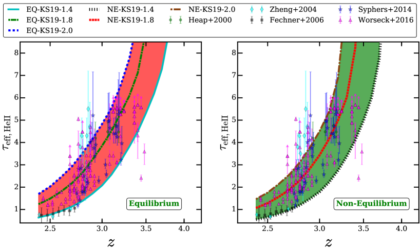
Appendix E Uncertainty in evolution of thermal history parameters

In this section we discuss the uncertainty in evolution of $T_{0}$ and $\gamma$ in the models L10-N512-G2-NE-KS19-1.4 (model NE-KS19-1.4 in main text of the paper). We run cite for L10-N512-G2 simulation from $z=6$ to $z=1.6$ due to limited storage and computational resources. At initial redshift ($z=6$ in L10-N512-G2 case), we assume a power-law TDR for $T_{0}$ and $\gamma$ consistent with gadget-3. It is important to study the effect of initial $T_{0}$ and $\gamma$ at $z=6$ on $T_{0}$ and $\gamma$ redshift at later epoch. We perform a low resolution L10-N128-G2 simulation to study the effect of initial $T_{0}$ and $\gamma$. We store the output for L10-N512-G2 simulation from $z=15$ to $z=1.6$ in steps of $\Delta z=0.1$. We post-process the output using cite, fit TDR at each redshift and calculate $T_{0}$, $\gamma$ evolution. Fig. 14 shows the $T_{0}$, $\gamma$ evolution from L10-N512-G2 and L10-N128-G2 models for HM12 equilibrium and non-equilibrium UVB cases. The $T_{0}$ and $\gamma$ evolution from the two models match within 8 percent.

Fig. 15 shows the $T_{0}$,$\gamma$ evolution for L10-N128-G2 simulation for KS19 equilibrium and non-equilibrium UVB cases. The $T_{0}$ and $\gamma$ evolution from $z=11$ to $z=6$ is very similar for equilibrium and non-equilibrium models. Furthermore, the $T_{0}$ and $\gamma$ evolution from $z=15$ to $z=6$ is very similar for different $\alpha$ values. This is expected as quasar contribution to UVB is not significant at high redshift. Thus the uncertainty in $T_{0}$, $\gamma$ (at $z=6$) due to differences in UVB is not significant.

In Fig. 16, we use measurements of $T_{0}$ at $z=6$ from observations of Bolton et al. (2012). We vary initial $T_{0}$ from 5000 to 9000 K in cite and calculate $T_{0}$,$\gamma$ evolution. Fig. 15 shows that even though the $\delta T_{0}=4000$ K at $z=6$ corresponds to lower $\delta T_{0}\sim 500$ K (maximum) at later redshift. Since the temperature has an uncertainty of the order of 5 percent, the corresponding uncertainty in $\Gamma_{\rm HI}$ would be $\sim 3.5$ percent.

In Fig. 17, we show the comparison of $T_{0}-\gamma$ measurements from observations with that from equilibrium and non-equilibrium models for $\alpha=1.8$ and $2.0$. The two models produce the $\tau_{\rm eff,HeII}$ evolution consistent with that from observations (see Fig. 7). The $T_{0}$ evolution from Walther et al. (2019) is in agreement within $1.5\sigma$ with L10-N512-NE-KS19-1.8 model. However, $\gamma$ evolution from Walther et al. (2019) is consistent within 2$\sigma$ with that from L10-N512-EQ-KS19-1.8 model.

Figure 14: Same as Fig. 4 except the $T_{0}$ and $\gamma$ evolution is shown for L10-N512-G2, L10-N128-G2 and SN (semi-numerical) simulations. In all cases, we use HM12 UVB and show $T_{0}$, $\gamma$ evolution for equilibrium and non-equilibrium ionization evolution. For L10-N128-G2-NE-HM12, L10-N128-G2-EQ-HM12, SN-EQ-HM12 and SN-NE-HM12 models we run cite from $z=15$ to $z=1.6$. While for L10-N512-G2-NE-HM12 and L10-N512-G2-EQ-HM12 models we run cite from $z=6$ to $z=2$. Figure shows that $T_{0}$, $\gamma$ evolution in low resolution (L10-N128-G2) simulation is consistent with high resolution (L10-N512-G2) simulation (differences less than 8 percent). Whereas the differences in high resolution simulation and semi-numerical method are less 11 percent. We use the low resolution simulation to study the effect of  H i reionization on $T_{0}$ and $\gamma$ values at $z=6$.

Figure 15: Same as Fig. 4 except the $T_{0}$ and $\gamma$ evolution is shown for L10-N128-G2-KS19-$\alpha$ simulations with $\alpha$ varying from 1.4 to 2.0. The $T_{0}$ and $\gamma$ values at $z=6$ are quite similar in all models indicating quasar SED has mild effect on $T_{0}$ and $\gamma$ evolution during  H i reionization. The $T_{0}$ and $\gamma$ values at $z=6$ in KS19 UVB model are less by 6.25 and 6.5 percent than that from HM12 UVB (not shown in figure) model respectively

Figure 16: Same as Fig. 4 except the $T_{0}$ and $\gamma$ evolution is shown for L10-N128-G2-KS19-1.4 simulations with variation in initial $T_{0}$ at $z=6$. We chose initial $T_{0}=5000$ and $9000$ K consistent with Bolton et al. (2012) $T_{0}$ measurement. Even though initial $T_{0}$ varied by $4000$ K, the corresponding maximum variation in $T_{0}$ is less than 500 K at $z<4.5$.

Figure 17: Comparison of $T_{0}$ and $\gamma$ evolution from KS19-1.8 and KS19-2.0 models with that from observations (Lidz et al., 2010; Becker et al., 2011; Boera et al., 2014; Hiss et al., 2018; Walther et al., 2019). The two models are shown for L10N512 simulation box and produce the $\tau_{\rm eff,HeII}$ evolution consistent with that from observations (see Fig. 7). The $T_{0}$ evolution from Walther et al. (2019) is in agreement (within $1.5\sigma$) with NE-KS19-1.8 model. However, $\gamma$ evolution from Walther et al. (2019) is consistent within 2$\sigma$ with that from EQ-KS19-1.8 model.

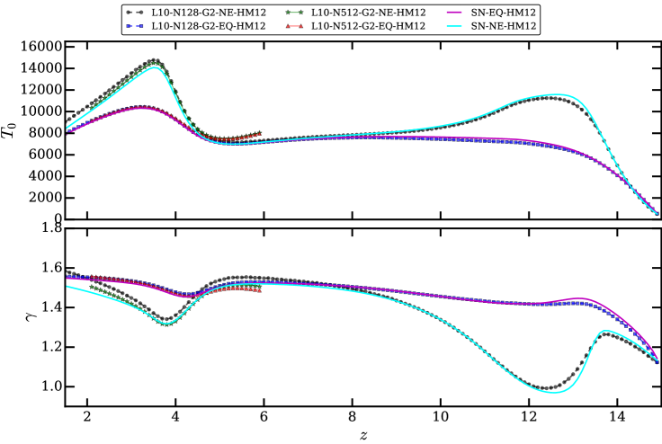
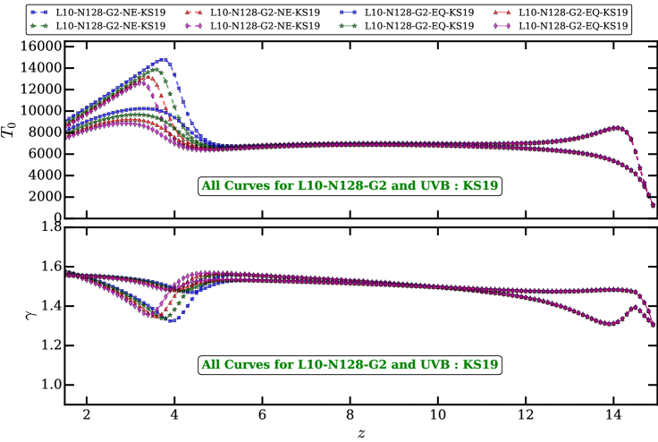
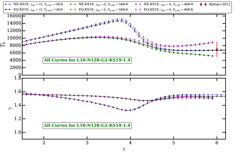
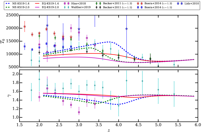
Appendix F  H i  Ly$\alpha$ flux statistics

Figure 18: Panels a,b show the FPDF, FPS respectively from equilibrium and non-equilibrium KS19 UVB models ($\alpha=1.4$) assuming constant $\Gamma_{\rm 12}$ $=1$. $\tau_{\rm eff,HI}$ is different for equilibrium and non-equilibrium models in this case. Panel c and d are similar to panel a and b respectively except that the $\tau_{\rm eff,HI}$ $=0.63$ is same for equilibrium and non-equilibrium models i.e., $\Gamma_{\rm 12}$ is different. Comparison of panel a and c suggests that non-equilibrium ionization evolution affect the $\Gamma_{\rm HI}$ measurements. However, the shape of the FPDF is not affected much. Panel b and d show that the non-equilibrium model has less power as compared to that for equilibrium model at scales $k>10\>h\>{\rm Mpc}^{-1}$ due to more pressure smoothing in non-equilibrium model ($T_{0}$ is larger in non-equilibrium models). All plots are shown for $z=3.6$.

In this section, we discuss the effect of non-equilibrium ionization evolution on  H i  Ly$\alpha$ flux statistics namely flux probability distribution function (FPDF) and flux power spectrum (FPS). The FPDF and FPS statistics are used in the past to constrain the $\Gamma_{\rm HI}$. Whereas FPS is sensitive to $T_{0}$ and $\gamma$. This is because for a given cosmology and ignoring the effect of thermal broadening and peculiar velocities, the  Ly$\alpha$ optical optical depth is given by (Weinberg et al., 1997),

$${}\tau_{\rm HI}\propto\frac{T_{0}^{-0.7}\>\Delta^{2-0.7(\gamma-1)}}{\Gamma_{\rm HI}}$$ (8)

where, $\Delta$ is overdensity and we assume that the  H ii recombination rate scales with temperature as $T^{-0.7}$. The above expression is an approximation and we do not use the for calculation of  Ly$\alpha$ optical depth in our simulated spectra.

The details on how to derive FPDF and FPS from  H i  Ly$\alpha$ forest spectra are discussed in G18. Here we briefly show the results for these statistics. Fig. 18 shows the two flux statistics for EQ-KS19-1.4 and NE-KS19-1.4 models. Panel a, b show the four statistics assuming a constant  H i photo-ionization rate ($\Gamma_{\rm 12}$ = 1) for two models. In this case, $\tau_{\rm eff,HI}$ for the two model is different. The bottom panels show the four statistics derived for EQ-KS19-1.4 and NE-KS19-1.4 models assuming $\tau_{\rm eff,HI}$ = 0.63. In this case, we vary $\Gamma_{\rm HI}$ to match the equilibrium and non-equilibrium model $\tau_{\rm eff,HI}$ with observed $\tau_{\rm eff,HI}$ = 0.63 at $z=3.6$ (Becker & Bolton, 2013). Panel a shows the case where $\tau_{\rm eff,HI}$ is different for EQ-KS19-1.4 and NE-KS19-1.4 models. The FPDF is quite different in two models. However when we match $\tau_{\rm eff,HI}$ (by changing $\Gamma_{\rm 12}$), the FPDF match very well as shown in panel c. This suggests that non-equilibrium / equilibrium ionization evolution does not affect the shape of the FPDF appreciably. The shape of the FPDF is relatively insensitive to $T_{0}$ and $\gamma$ parameters. Since the thermal history is significantly different for equilibrium and non-equilibrium model (see Fig. 4), one expects to see the differences in FPS. On smaller scales ($k>10\>h\>{\rm Mpc}^{-1}$), the power in non-equilibrium model is smaller than that for equilibrium model. This is because of pressure smoothing is more in non-equilibrium model (since $T_{0}$ is larger) as compared to equilibrium model. We again see that the match between EQ-KS19-1.4 and NE-KS19-1.4 model is relatively good when $\tau_{\rm eff,HI}$ between two models is same (compare panel b and d in Fig. 18). Thus non-equilibrium effects during  He ii reionization does not appreciably change the shapes FPDF and FPS derived from  H i  Ly$\alpha$ forest. However, the equilibrium and non-equilibrium processes affect the thermal history of IGM.

References

- Aubert & Teyssier (2008) Aubert D., Teyssier R., 2008, MNRAS, 387, 295
- Avni (1976) Avni Y., 1976, ApJ, 210, 642
- Becker & Bolton (2013) Becker G. D., Bolton J. S., 2013, MNRAS, 436, 1023
- Becker et al. (2011) Becker G. D., Bolton J. S., Haehnelt M. G., Sargent W. L. W., 2011, MNRAS, 410, 1096
- Becker et al. (2013) Becker G. D., Hewett P. C., Worseck G., Prochaska J. X., 2013, MNRAS, 430, 2067
- Becker et al. (2015) Becker G. D., Bolton J. S., Madau P., Pettini M., Ryan-Weber E. V., Venemans B. P., 2015, MNRAS, 447, 3402
- Bernardi et al. (2003) Bernardi M., et al., 2003, AJ, 125, 32
- Boera et al. (2014) Boera E., Murphy M. T., Becker G. D., Bolton J. S., 2014, MNRAS, 441, 1916
- Bolton & Haehnelt (2007) Bolton J. S., Haehnelt M. G., 2007, MNRAS, 382, 325
- Bolton et al. (2008) Bolton J. S., Viel M., Kim T.-S., Haehnelt M. G., Carswell R. F., 2008, MNRAS, 386, 1131
- Bolton et al. (2012) Bolton J. S., Becker G. D., Raskutti S., Wyithe J. S. B., Haehnelt M. G., Sargent W. L. W., 2012, MNRAS, 419, 2880
- Bolton et al. (2017) Bolton J. S., Puchwein E., Sijacki D., Haehnelt M. G., Kim T.-S., Meiksin A., Regan J. A., Viel M., 2017, MNRAS, 464, 897
- Choudhury et al. (2001) Choudhury T. R., Srianand R., Padmanabhan T., 2001, ApJ, 559, 29
- Cohen et al. (1996) Cohen S. D., Hindmarsh A. C., Dubois P. F., 1996, Computers in Physics, 10, 138
- D’Aloisio et al. (2018) D’Aloisio A., McQuinn M., Maupin O., Davies F. B., Trac H., Fuller S., Upton Sanderbeck P. R., 2018, arXiv e-prints,
- Davies et al. (2017) Davies F. B., Furlanetto S. R., Dixon K. L., 2017, MNRAS, 465, 2886
- Dayal & Ferrara (2018) Dayal P., Ferrara A., 2018, Phys. Rep., 780, 1
- Dixon et al. (2014) Dixon K. L., Furlanetto S. R., Mesinger A., 2014, MNRAS, 440, 987
- Fan et al. (2001) Fan X., et al., 2001, AJ, 122, 2833
- Fan et al. (2006) Fan X., et al., 2006, AJ, 132, 117
- Faucher-Giguère et al. (2008a) Faucher-Giguère C.-A., Lidz A., Hernquist L., 2008a, Science, 319, 52
- Faucher-Giguère et al. (2008b) Faucher-Giguère C.-A., Prochaska J. X., Lidz A., Hernquist L., Zaldarriaga M., 2008b, ApJ, 681, 831
- Faucher-Giguère et al. (2008c) Faucher-Giguère C.-A., Lidz A., Hernquist L., Zaldarriaga M., 2008c, ApJ, 682, L9
- Fechner et al. (2006) Fechner C., et al., 2006, A&A, 455, 91
- Furlanetto & Oh (2008) Furlanetto S. R., Oh S. P., 2008, ApJ, 681, 1
- Gaikwad et al. (2017) Gaikwad P., Khaire V., Choudhury T. R., Srianand R., 2017, MNRAS, 466, 838
- Gaikwad et al. (2018) Gaikwad P., Choudhury T. R., Srianand R., Khaire V., 2018, MNRAS, 474, 2233
- Garzilli et al. (2012) Garzilli A., Bolton J. S., Kim T.-S., Leach S., Viel M., 2012, MNRAS, 424, 1723
- Giallongo et al. (2015) Giallongo E., et al., 2015, A&A, 578, A83
- Gnedin (2014) Gnedin N. Y., 2014, ApJ, 793, 29
- Gnedin & Hui (1998) Gnedin N. Y., Hui L., 1998, MNRAS, 296, 44
- Haardt & Madau (1996) Haardt F., Madau P., 1996, ApJ, 461, 20
- Haardt & Madau (2012) Haardt F., Madau P., 2012, ApJ, 746, 125
- Heap et al. (2000) Heap S. R., Williger G. M., Smette A., Hubeny I., Sahu M. S., Jenkins E. B., Tripp T. M., Winkler J. N., 2000, ApJ, 534, 69
- Hiss et al. (2018) Hiss H., Walther M., Hennawi J. F., Oñorbe J., OMeara J. M., Rorai A., Lukic Z., 2018, ApJ, 865, 42
- Hui & Gnedin (1997) Hui L., Gnedin N. Y., 1997, MNRAS, 292, 27
- Jakobsen et al. (1994) Jakobsen P., Boksenberg A., Deharveng J. M., Greenfield P., Jedrzejewski R., Paresce F., 1994, Nature, 370, 35
- Katz et al. (1996) Katz N., Weinberg D. H., Hernquist L., 1996, ApJS, 105, 19
- Keating et al. (2018) Keating L. C., Puchwein E., Haehnelt M. G., 2018, MNRAS, 477, 5501
- Khaire (2017) Khaire V., 2017, MNRAS, 471, 255
- Khaire & Srianand (2013) Khaire V., Srianand R., 2013, MNRAS, 431, L53
- Khaire & Srianand (2015a) Khaire V., Srianand R., 2015a, MNRAS, 451, L30
- Khaire & Srianand (2015b) Khaire V., Srianand R., 2015b, ApJ, 805, 33
- Khaire & Srianand (2019) Khaire V., Srianand R., 2019, MNRAS, 484, 4174
- Khaire et al. (2016) Khaire V., Srianand R., Choudhury T. R., Gaikwad P., 2016, MNRAS, 457, 4051
- Kriss et al. (2001) Kriss G. A., et al., 2001, Science, 293, 1112
- Kulkarni et al. (2015) Kulkarni G., Hennawi J. F., Oñorbe J., Rorai A., Springel V., 2015, ApJ, 812, 30
- Kulkarni et al. (2018) Kulkarni G., Worseck G., Hennawi J. F., 2018, preprint, (arXiv:1807.09774)
- La Plante & Trac (2016) La Plante P., Trac H., 2016, ApJ, 828, 90
- La Plante et al. (2017) La Plante P., Trac H., Croft R., Cen R., 2017, ApJ, 841, 87
- La Plante et al. (2018) La Plante P., Trac H., Croft R., Cen R., 2018, ApJ, 868, 106
- Lidz et al. (2010) Lidz A., Faucher-Giguère C.-A., Dall’Aglio A., McQuinn M., Fechner C., Zaldarriaga M., Hernquist L., Dutta S., 2010, ApJ, 718, 199
- Lukić et al. (2015) Lukić Z., Stark C. W., Nugent P., White M., Meiksin A. A., Almgren A., 2015, MNRAS, 446, 3697
- Lusso et al. (2015) Lusso E., Worseck G., Hennawi J. F., Prochaska J. X., Vignali C., Stern J., O’Meara J. M., 2015, MNRAS, 449, 4204
- Lusso et al. (2018) Lusso E., Fumagalli M., Rafelski M., Neeleman M., Prochaska J. X., Hennawi J. F., O’Meara J. M., Theuns T., 2018, ApJ, 860, 41
- Madau & Haardt (2015) Madau P., Haardt F., 2015, ApJ, 813, L8
- McDonald et al. (2000) McDonald P., Miralda-Escudé J., Rauch M., Sargent W. L. W., Barlow T. A., Cen R., Ostriker J. P., 2000, ApJ, 543, 1
- McDonald et al. (2005) McDonald P., et al., 2005, ApJ, 635, 761
- Oñorbe et al. (2017) Oñorbe J., Hennawi J. F., Lukić Z., 2017, ApJ, 837, 106
- Oppenheimer & Schaye (2013) Oppenheimer B. D., Schaye J., 2013, MNRAS, 434, 1043
- Padmanabhan et al. (2015) Padmanabhan H., Srianand R., Choudhury T. R., 2015, MNRAS, 450, L29
- Penton et al. (2000) Penton S. V., Shull J. M., Stocke J. T., 2000, ApJ, 544, 150
- Phillips et al. (2001) Phillips J., Weinberg D. H., Croft R. A. C., Hernquist L., Katz N., Pettini M., 2001, ApJ, 560, 15
- Planck Collaboration et al. (2014) Planck Collaboration et al., 2014, A&A, 571, A16
- Press et al. (1992) Press W. H., Teukolsky S. A., Vetterling W. T., Flannery B. P., 1992, Numerical recipes in FORTRAN. The art of scientific computing
- Puchwein et al. (2015) Puchwein E., Bolton J. S., Haehnelt M. G., Madau P., Becker G. D., Haardt F., 2015, MNRAS, 450, 4081
- Puchwein et al. (2019) Puchwein E., Haardt F., Haehnelt M. G., Madau P., 2019, MNRAS, 485, 47
- Rosdahl et al. (2013) Rosdahl J., Blaizot J., Aubert D., Stranex T., Teyssier R., 2013, MNRAS, 436, 2188
- Rudie et al. (2012) Rudie G. C., Steidel C. C., Pettini M., 2012, ApJ, 757, L30
- Schaye et al. (2000) Schaye J., Theuns T., Rauch M., Efstathiou G., Sargent W. L. W., 2000, MNRAS, 318, 817
- Scoccimarro et al. (2012) Scoccimarro R., Hui L., Manera M., Chan K. C., 2012, Phys. Rev. D, 85, 083002
- Shull et al. (2004) Shull J. M., Tumlinson J., Giroux M. L., Kriss G. A., Reimers D., 2004, ApJ, 600, 570
- Shull et al. (2012a) Shull J. M., Harness A., Trenti M., Smith B. D., 2012a, ApJ, 747, 100
- Shull et al. (2012b) Shull J. M., Smith B. D., Danforth C. W., 2012b, ApJ, 759, 23
- Springel (2005) Springel V., 2005, MNRAS, 364, 1105
- Stevans et al. (2014) Stevans M. L., Shull J. M., Danforth C. W., Tilton E. M., 2014, ApJ, 794, 75
- Syphers & Shull (2014) Syphers D., Shull J. M., 2014, ApJ, 784, 42
- Theuns et al. (1998) Theuns T., Leonard A., Efstathiou G., Pearce F. R., Thomas P. A., 1998, MNRAS, 301, 478
- Theuns et al. (2002) Theuns T., Zaroubi S., Kim T.-S., Tzanavaris P., Carswell R. F., 2002, MNRAS, 332, 367
- Tilton et al. (2016) Tilton E. M., Stevans M. L., Shull J. M., Danforth C. W., 2016, ApJ, 817, 56
- Viel et al. (2004) Viel M., Haehnelt M. G., Springel V., 2004, MNRAS, 354, 684
- Walther et al. (2019) Walther M., Oñorbe J., Hennawi J. F., Lukić Z., 2019, ApJ, 872, 13
- Weinberg et al. (1997) Weinberg D. H., Hernquist L., Katz N., 1997, ApJ, 477, 8
- Weinberg et al. (1998) Weinberg D. H., Katz N., Hernquist L., 1998, in Woodward C. E., Shull J. M., Thronson Jr. H. A., eds, Astronomical Society of the Pacific Conference Series Vol. 148, Origins. p. 21 (arXiv:astro-ph/9708213)
- Worseck et al. (2011) Worseck G., et al., 2011, ApJ, 733, L24
- Worseck et al. (2016) Worseck G., Prochaska J. X., Hennawi J. F., McQuinn M., 2016, ApJ, 825, 144
- Worseck et al. (2018) Worseck G., Davies F. B., Hennawi J. F., Prochaska J. X., 2018, preprint, (arXiv:1808.05247)
- Zaldarriaga (2002) Zaldarriaga M., 2002, ApJ, 564, 153
- Zheng et al. (2004) Zheng W., et al., 2004, ApJ, 605, 631