Blue-Noise Sampling on Graphs

Abstract

In the area of graph signal processing, a graph is a set of nodes arbitrarily connected by weighted links; a graph signal is a set of scalar values associated with each node; and sampling is the problem of selecting an optimal subset of nodes from which a graph signal can be reconstructed. This paper proposes the use of spatial dithering on the vertex domain of the graph, as a way to conveniently find statistically good sampling sets. This is done establishing that there is a family of good sampling sets characterized on the vertex domain by a maximization of the distance between sampling nodes; in the Fourier domain, these are characterized by spectrums that are dominated by high frequencies referred to as blue-noise. The theoretical connection between blue-noise sampling on graphs and previous results in graph signal processing is also established, explaining the advantages of the proposed approach. Restricting our analysis to undirected and connected graphs, numerical tests are performed in order to compare the effectiveness of blue-noise sampling against other approaches.

I Introduction

Interesting phenomena in nature can often be captured by graphs since objects and data are invariably inter-related in some sense. Social [1], financial [2], ecological networks, and the human brain [3] are a few examples of such networks. Data in these networks reside on irregular or otherwise unordered structures [4]. New data science tools are thus emerging to process signals on graph structures where concepts of algebraic and spectral graph theory are being merged with methods used in computational harmonic analysis [5, 6, 7]. A common problem in these networks is to determine which nodes play the most important role, assuming there is a quantity of interest defined on the network.

Graph signal sampling thus becomes essential. Naturally, the mathematics of sampling theory and spectral graph theory have been combined leading to generalized Nyquist sampling principles for graphs [5, 8, 9, 10, 11, 12]. In general, these methods are based on the underlying graph spectral decompositions [12, 13, 14, 15].

This work explores a somewhat radical departure from prior work, inspired by sampling patterns in traditional dithering and halftoning. Specifically, we intend to design graph signal sampling techniques that promote the maximization of the distance between sampling nodes on the vertex domain that are typically characterized by a low frequency energy. Sampling patterns with these characteristics are referred to in the spatial dithering literature as blue-noise [16, 17].

In this paper, the connection between the properties of blue-noise sampling patterns and the results related with sampling sets in graphs is established, showing that blue-noise like sampling patterns in graphs are connected with good sampling sets in terms of preserving the uniqueness of the representation of the sampled signal in a noise-free scenario. Additionally, it is shown how the inter-distance between the sampling nodes affects the redness in a given sampling pattern. We provide a measure of the bandwidth of the signals that can be uniquely represented from the vertex-domain characteristics of blue-noise sampling patterns. A numerical algorithm is proposed in order to compute these blue-noise patterns based on their vertex-domain distribution. In particular, trying to exploit the distribution of the sampling points on the nodes of the graph, a void and cluster algorithm on graphs is developed [18], allowing the generation of patterns that lead to reconstruction errors of bandlimited signals, similar to the ones obtained in the state-of-the-art literature.

This work is organized as follows: in Section II, notation and basic concepts about signal processing on graphs are stated presenting also a description of previous approaches about sampling on graphs. In Section III blue-noise sampling on graphs is discussed. In Section IV an algorithm for the generation of blue-noise patterns is discussed, whereas in Section V a set of numerical tests show the performance of the proposed algorithm against other techniques. Finally, in Section VI a set of conclusions is presented.

II Preliminaries

Sandryhaila [19] proposed a theoretical framework for the analysis and processing of signals on graphs based on the properties of the adjacency matrix. This approach is rooted in algebraic signal processing, whereas authors like Fuhr and Pesenson [8, 9, 20], Puy [21] and Shuman [5, 6, 22] based their analysis of signals on graphs, relying on the properties of the Laplacian matrix. In both approaches the Fourier transform of the signals on the graph is defined in terms of a spectral decomposition of the adjacency matrix and the Laplacian matrix respectively, using the set of eigenvectors as the Fourier basis for the representation of the signals.

The first approach offers a direct connection with the shift operator used in traditional signal processing, while the second resembles the main ideas of Fourier analysis in linear spaces in which the eigenfunctions of the Laplacian operator are used as the basis representation of the signal. The two approaches use a unitary operator, and problems like sampling and filtering can be successfully considered in both scenarios. In this work, the combinatorial Laplacian matrix is used as the building block, and the graphs considered are undirected, weighted, connected and simple. Consequently, part of the developments proposed rely on the theoretical results obtained by Furh and Pesenson [8, 9, 20] in harmonic analysis on graphs.

II-A Graph Signal Sampling

Let $G=\left(V(G),E(G)\right)$ be an undirected, weighted, connected, simple graph with a set of nodes, $V(G)$, and a set of edges, $E(G)$. $\mathbf{W}$ is the adjacency matrix (symmetric), with $\mathbf{W}(u,v)\geq 0$ the weight connecting the nodes $u$ and $v$ and $u\sim v$ indicates that $\mathbf{W}(u,v)>0$. The degree matrix, $\mathbf{D}$, is a diagonal matrix whose entries are given according to:

$$\mathbf{D}(u,u)=\sum_{v\in V(G)}\mathbf{W}(u,v).$$ (1)

For any graph $G$, its volume is defined as $vol(G)=\sum_{u\in V(G)}\mathbf{D}(u,u)$, and the volume of a subset $S\subset V(G)$ is defined as $vol(S)=\sum_{u\in S}\mathbf{D}(u,u)$. On the graph $G$, the combinatorial Laplacian operator is defined as the positive semi-definite operator:

$$\mathbf{L}=\mathbf{D}-\mathbf{W},$$ (2)

whose eigenvalues are organized as $0\leq\mu_{1}\leq\mu_{2}\leq\ldots\leq\mu_{N}$, $N=|V(G)|$ [23]. A real signal, $\boldsymbol{x}$, on the graph is then defined as the mapping $\boldsymbol{x}:V(G)\longrightarrow\mathbb{R}$ represented by the vector $\boldsymbol{x}\in\mathbb{R}^{N}$ where $\boldsymbol{x}(v)$ is the value of the signal associated to $v\in V(G)$. The support of $\boldsymbol{x}$ is represented as $\operatorname{supp}(\boldsymbol{x})$, and the restriction of $\boldsymbol{x}$, to any subset $S\subset V(G)$, is represented as $\boldsymbol{x}(S)$. It is worth noticing that:

$$(\mathbf{L}\boldsymbol{x})(v)=\sum_{u\in V(G)}\left(\boldsymbol{x}(v)-\boldsymbol{x}(u)\right)\mathbf{W}(v,u).$$ (3)

If the spectral decomposition of the operator $\mathbf{L}$ is represented as $\mathbf{L}=\mathbf{U}\boldsymbol{\Lambda}\mathbf{U}^{\mathsf{T}}$, then the Graph Fourier Transform (GFT) of the signal, $\boldsymbol{x}$ on $G$, is given by $\hat{\boldsymbol{x}}=\mathbf{U}^{\mathsf{T}}\boldsymbol{x}$. There is a direct analogy between the concept of frequency in traditional Fourier Analysis and the behavior of the Graph Fourier Transform as is stated in [5]. Considering this analogy, the bandwidth of a signal $\boldsymbol{x}$ can be defined using the nonzero components of $\hat{\boldsymbol{x}}$. It is said that $\boldsymbol{x}$ has bandwidth $\omega\in\mathbb{R}_{+}$ on the spectral axes if $\hat{\boldsymbol{x}}\in PW_{\omega}(G)=\text{span}\{\mathbf{U}_{k}:\mu_{k}\leq\omega\}$, where $PW_{\omega}(G)$ is the Paley-Wiener space of bandwidth $\omega$ [8] and $\mathbf{U}_{k}$ indicates the first $k$ column vectors in $\mathbf{U}$. In some cases the bandwidth is also represented with the largest integer $k$ such that $\mu_{k}\leq\omega$.

Given a notion of bandwidth, one invariably questions the notion of sampling rate and whether the number of samples or nodes of a graph can be reduced without loss of information to the signal. We, therefore, define sampling of a signal $\boldsymbol{x}$ on the graph $G$, by choosing the components of $\boldsymbol{x}$ on a subset of nodes, $S=\{s_{1},\ldots,s_{m}\}\subset V(G)$. The sampled signal is given by $\boldsymbol{x}(S)=\mathbf{M}\boldsymbol{x}$ where $\mathbf{M}$ is a binary matrix whose entries are given by $\mathbf{M}=[\boldsymbol{\delta}_{s_{1}},\ldots,\boldsymbol{\delta}_{s_{m}}]^{\mathsf{T}}$ and $\boldsymbol{\delta}_{v}$ is the $N-$ dimensional Kronecker column vector centered at $v$. Given $\boldsymbol{x}(S)$, it is possible to obtain a reconstructed version of $\boldsymbol{x}$ in different ways depending on whether the bandwidth of the signal is known. We assume that the bandwidth is known and that the reconstruction is given by:

$$\boldsymbol{x}_{rec}=\operatorname*{argmin}_{\boldsymbol{z}\in span(\mathbf{U}_{k})}\|\mathbf{M}\boldsymbol{z}-\boldsymbol{x}(S)\|^{2}_{2}=\mathbf{U}_{k}\left(\mathbf{M}\mathbf{U}_{k}\right)^{\dagger}\boldsymbol{x}(S)$$ (4)

where $\left(\mathbf{M}\mathbf{U}_{k}\right)^{\dagger}$ is the Moore-Penrose pseudo-inverse of $\mathbf{M}\mathbf{U}_{k}$ [24, 25]. Alternatively, in [26] it is shown that a consistent reconstruction of the signal can be obtained from its samples using interpolation splines.

The problem of optimally sampling a signal on a graph can now be summarized as choosing $S$ such that we maximize the available bandwidth of $\boldsymbol{x}(S)$. To this end, Pesenson defines [8, 9] a $\Lambda$-removable set for $\Lambda>0$ as the subset of nodes, $S\subset V(G)$, for which:

$$\|\boldsymbol{x}\|_{2}\leq(1/\Lambda)\|\mathbf{L}\boldsymbol{x}\|_{2}\quad\quad\forall~{}\boldsymbol{x}\in L_{2}(S),$$ (5)

where $L_{2}(S)$ is the set of all signals, $\boldsymbol{x}$, with support in $S\subset V(G)$ (i.e. elements of $\boldsymbol{x}$ not included in $S$ are equal to zero) and finite $\ell_{2}$ norm. The largest value of $\Lambda$ for which eqn. (5) holds is denoted by $\Lambda_{S}$. Notice that for any subset of nodes there exists a $\Lambda$-removable set with larger or smaller $\Lambda_{S}$. Therefore, $\Lambda_{S}$ ultimately determines how much importance a given set has in the sampling process of a signal with a specific bandwidth. The relationship between properties of removable sets and the sampling problem was established by Pesenson in the following theorem:

Theorem 1 (Theorem 5.1 in [8])

If for a set $S\subset V(G)$, its compliment $S^{c}=V(G)\setminus S$ is a $\Lambda_{S^{c}}-$removable set, then all signals in $PW_{\omega}(G)$ are completely determined by its values in $S$, whenever $0<\omega<\Lambda_{S^{c}}$.

In [20], another result related with sampling sets is established using a constant that can be calculated directly with the weights, $\mathbf{W}$, of the graph, $G$, stated in the following theorem:

Theorem 2 ([20])

Every $S\subset V(G)$ is a uniqueness set for all functions in $PW_{\omega}(G)$ with any $\omega<K_{S}$, where

$$K_{S}=\inf_{v\in S^{c}}w_{S}(v)$$ (6)

and $w_{S}(v)=\sum_{s\in S}\mathbf{W}(s,v)$.

Theorems 1 and 2 play a central role in the description of properties for different classes of sampling sets as it is possible to consider that a good sampling set, $S$, promotes the maximization of constants, $\Lambda_{S^{c}}$ and $K_{S}$. In particular, it will be shown in the following sections that blue-noise sampling patterns indeed promote high values of these constants.

Recently Pesenson [27] introduced results that characterize the representation of a band limited signal in terms of induced subgraphs obtained from partitions of $V(G)$ that cover $V(G)$. This statement can be summarized in the following theorem.

Theorem 3 (5.1,6.1,6.2 [27])

Let $G$ be a connected finite or infinite and countable graph. Suppose that $\mathcal{P}=\{V(\Omega_{j})\}_{j=1}^{j=|\mathcal{P}|}$ is a disjoint cover of $V(G)$ by connected and finite subgraphs $\Omega_{j}$. Let $\mathbf{L}_{\Omega_{j}}$ be the Laplace operator of the induced graph $\Omega_{j}$ whose first nonzero eigenvalue is $\mu_{1,j}$. If $\Lambda_{\mathcal{P}}=\inf_{j}\mu_{1,j}>0$ and $\Lambda_{\mathcal{P}}>\frac{1+\alpha}{\alpha}\omega$ with $\alpha>0$, then every signal $\boldsymbol{x}\in PW_{\omega}(G)$ is uniquely determined by the values $\boldsymbol{x}^{\mathsf{T}}\boldsymbol{\xi}_{j}$, where $\boldsymbol{\xi}_{j}=\boldsymbol{\chi}_{j}/\sqrt{|V(\Omega_{j})|}$ with $\boldsymbol{\chi}_{j}(V(\Omega_{j}))=1$ and $\boldsymbol{\chi}_{j}(V(\Omega_{j})^{c})=0$. Additionally, $\boldsymbol{x}$ can be reconstructed from this set of values in a stable way.

It is important to remark the meaning and implications of Theorem 3. This result shows that $V(G)$ can be divided into disjoint subsets that cover $V(G)$, and a given band limited signal can be reconstructed from the average values of the signal in those regions. Additionally, the constant $\Lambda_{\mathcal{P}}$ associated to the partition provides a measure of the quality of the reconstruction obtained from the regions on $V(G)$ defined by $\mathcal{P}$. It is also worthy to point out that the size of the elements in the partition has a natural limit as $\mathbf{L}_{\Omega_{j}}$ is expected to have at least one nonzero eigenvalue, which would not be the case when $\Omega_{j}$ consist of one single vertex. This result will allow us to establish a connection between the spectral and vertex domain behavior of sampling patterns in some classes of graphs. Additionally, we will show that from a blue-noise sampling pattern $\boldsymbol{s}$, it is possible to build a partition that can be used to estimate the bandwidth of signals that are uniquely represented by their samples on the sampling nodes indicated by $\boldsymbol{s}$.

II-B Optimal Graph Sampling

The problem of finding the best $S$ is a combinatorial problem of calculating $\Lambda_{S^{c}}$ for all sampling sets and choosing the set with the largest value of $\Lambda_{S^{c}}$, a prohibitively expensive process for large graphs. Allowing for some short cuts, a simple, greedy procedure for finding a good sampling set starts with an empty set of nodes and iteratively adds one node at a time, taking the best available node at each iteration according the value of a cost function. Several authors have formulated the problem of sampling and reconstruction in the presence of measurement noise, and in these works objective functions have been proposed that minimize the reconstruction error in terms of the worst case [14], where $S^{opt}=\arg\max_{|S|=m}\sigma_{1}^{2}$, the mean case [24], where $S^{opt}=\arg\max_{|S|=m}\sum_{i=1}^{\min\{m,k\}}\sigma_{i}^{-2}$, and the maximum volume case [25], where $S^{opt}=\arg\max_{|S|=m}\prod_{i=1}^{\min\{m,k\}}\sigma_{i}^{2}$; and $\sigma_{i}$ represents the $i^{th}$ singular value of the matrix $\mathbf{M}\mathbf{U}_{k}$ consisting of the first $k$ eigenvectors of ${\bf W}$ or ${\bf L}$ respectively, sampled on the rows indicated by $S$. In [28] the optimal sampling set is obtained considering the same cost function for the mean case, but using the singular values of $\mathbf{\Lambda}\mathbf{U}^{\mathsf{T}}\text{diag}(S)$, where $\text{diag}(S)$ is the diagonal matrix whose entries are given by $\text{diag}(S)_{i,i}=1\Leftrightarrow i\in S$.

In order to reduce computational complexity, Anis et. al. [24] defines graph spectral proxies of order $q$ as estimates of the cutoff frequency of a given signal which can be used to define cutoff frequency estimates for a subset of nodes $S$ according to:

$$\Omega_{q}(S)=\min_{\phi\in L_{2}(S^{c})}\left(\frac{\|{\bf L}^{k}\phi\|_{2}}{\|\phi\|_{2}}\right)^{\frac{1}{q}},$$ (7)

with $\mathbf{L}^{q}$ being the $q^{th}$ power of $\mathbf{L}$ [24, 13]. Anis et. al. further shows that, for any $q\in\mathbb{N}$ and $S$, it is possible to have perfect reconstruction when $\omega<\Omega_{q}(S)$. The value of $\Omega_{q}(S)$ can be calculated as $\Omega_{q}(S)=(\sigma_{1,q})^{\frac{1}{2q}}$, where $\sigma_{1,q}$ denotes the smallest eigenvalue of the reduced matrix $\mathbf{L}^{2q}_{S^{c},S^{c}}$. The optimal sampling set can then be represented as the solution of the problem:

$$S_{q}^{opt}=\arg\max_{|S|=m}\Omega_{q}(S),$$ (8)

which is still combinatorial; however, Anis et. al. proposes a heuristic rule to solve eqn. (8) using the first eigenvector of ${\bf L}^{q}_{S^{c},S^{c}}$. Basically, a node is added to the sampling set according to the index of the component with maximum absolute value for the first eigenvector of ${\bf L}^{q}_{S^{c},S^{c}}$. The quality of the sampling set is also related to the value of $q$, which should be selected as large as possible at the expense of a higher computational cost. In [29], some performance theoretical bounds for these greedy sampling techniques are derived.

In some scenarios for sampling signals on graphs a spectral decomposition of the operators is not available, and therefore, there is a strong need for vertex domain sampling schemes that attempt to build good sampling patterns based entirely on the local graph structure around a node. In particular, for those cases where the graphs are too large for calculating the eigenvalues and eigenvectors of the GFT, several authors have looked at the problem of sampling using subsets of nodes that may not be optimal but are still very good at preserving band-limited signals. In the case of Puy et. al [21], the authors perform a random selection of nodes with a recovery algorithm that involves a probability distribution on a diagonal matrix, ${\bf P}$, in addition to the sampling matrix operator $\mathbf{M}$. The reconstructed signal $\boldsymbol{x}_{rec}$ can then be calculated as:

$$\boldsymbol{x}_{rec}=\arg\min_{\boldsymbol{z}\in\mathbb{R}^{N}}\left(\left\|{\bf P}^{-1/2}({\bf M}\boldsymbol{z}-\boldsymbol{x}(S))\right\|^{2}_{2}+\tau\boldsymbol{z}^{\intercal}{g(\bf L})\boldsymbol{z}\right),$$ (9)

where $\boldsymbol{x}(S)={\bf M}\boldsymbol{x}$ is the sampled version of the signal $\boldsymbol{x}$, $\tau$ is a regularization parameter selected empirically and $g(\cdot)$ is a polynomial function selected also empirically.

Puy et. al [21] further show that an optimal ${\bf P}$ can be determined by the use of the local graph coherence, $\nu_{k}$, on the nodes of the graph. The value of $\nu_{k}(i)$ at the node $i$ can be calculated as $\nu_{k}(i)=\|{\bf U}_{k}\boldsymbol{\delta}_{i}\|_{2}$, where $\boldsymbol{\delta}_{i}$ is the Kronecker vector centered at node $i$, and it provides a measure about how important is the node $i$ for the sampling of a signal with bandwidth $k$. If $\nu_{k}(i)$ is equal to 1 for a particular node $i$, then there exists $k$-bandlimited graph signals whose energy is solely concentrated in this $i^{th}$ node. If $\nu_{k}(i)$ is equal to 0, then no $k$-bandlimited graph signal has any energy in this $i^{th}$ node. Therefore, node $i$ can be deleted with no repercussions.

Because the calculation of $\nu_{k}(i)$ requires the knowledge of the spectral decomposition, Puy et. al propose an approximate estimation of $\nu_{k}(i)$ that can be obtained without the calculation of any spectral decomposition, which allows the solution of eqn. (9). When the optimal ${\bf P}$ is used, Puy et. al show that the matrix ${\bf M}{\bf P}^{-1/2}$ satisfies a restricted isometry property when the number of samples is on the order of $O(k\log k)$, which provides a strong guarantee for the exact recovery of the signal. This represents an elegant result but with the drawback that $O(k\log k)$ is substantially higher than $k$, which is the optimal number of samples required to reconstruct a signal of bandwidth $k$.

Recently, Tremblay et. al. [25] proposed the use of determinantal point processes (DPP) in order to obtain the matrix ${\bf P}$ used in [21]. It is shown in [25] that an optimal ${\bf P}$ can be obtained using DPP when ${\bf U}_{k}$ is known. Additionally, when the spectral decomposition is not accessible, it is shown how a variant of the Wilson’s Algorithm introduced in [30] can be used in order to obtain a sampling set that can be shown is related with a DPP that leads to an approximate version of the optimal ${\bf P}$. The reconstruction of the signal is obtained by as solution of eqn. (9); however, these results do not represent an improvement with respect to Anis et. al. [24] or Chen et. al. [14] and may lead to larger reconstruction errors when the graph considered does not have a strong community graph structure [25]. Wang et. al. [31] consider the sampling and reconstruction of signals adapting concepts and ideas from frame theory, developing an iterative approach based on the concept of local sets.

Marques et. al. [32], proposed a different approach with respect to previous works, considering the sampling and reconstruction of the signal using its samples on a single node. The central idea is based on the information provided by the sequential application of the shift operator. The technique itself represents a novel alternative with potential applications in network analysis and its computational cost may be a drawback when large size graphs are considered.

III Blue-noise Sampling on Graphs

This work proposes a different approach to graph signal sampling: the application of spatial dithering to the graph vertex domain where the spectral properties of well formed sampling patterns will equally benefit the graph vertex domain as they do the spatial. This approach is motivated by the well established research in digital halftoning, which is the process of converting a continuous tone image or photograph into a pattern of printed and not-printed dots for reproduction by inkjet or laser printers [16, 17, 33]. Halftoning algorithms based on error-diffusion are of particular importance because they produce random patterns of homogeneously distributed dots where minority pixels (black dots in highlights or white dots in shadows) are spaced as far apart as possible. These patterns have power spectra dominated by high frequency energy, earning the name, “blue-noise,” since blue is the high frequency component of white light. Low frequency energy or red-noise contributes to halftone patterns looking fuzzy or noisy to the human visual system and are, therefore, to be avoided [16, 33].

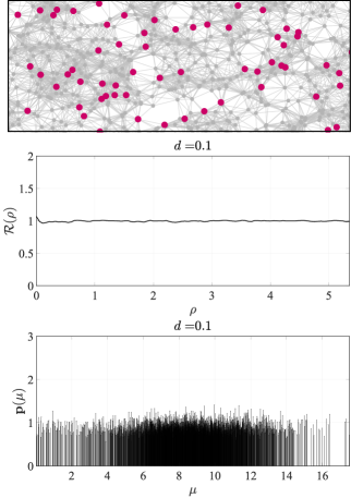
In order to establish a blue-noise model for sampling signals on a graph, we first propose the idea of a binary dither pattern on a graph, $G=(V(G),E(G))$, as the binary graph signal, $\boldsymbol{s}\in\{0,1\}^{N}$. We refer to the fraction of samples that we intend to preserve as the density $d=m/N$, where $\|\boldsymbol{s}\|_{0}=m$. In the case of a white-noise dither pattern as illustrated in Fig. 1 (top) on a Sensor Network graph for $d=0.1$, $\boldsymbol{s}$ is selected uniformly at random from the space of binary signals for which $\|\boldsymbol{s}\|_{0}=dN$; therefore each component of $\boldsymbol{s}$ can be modeled as a Bernoulli random variable with expected value $\mathbb{E}\{\boldsymbol{s}(\ell)\}=d$.

III-A Vertex-domain Characteristics

Figure 1: Illustration of the spatial and spectral properties of (top) a white-noise dither pattern on a Sensor Network graph with density, $d=0.1$, with (center) a flat pair correlation approximately equal to 1.0 for all internode distances, $\rho$, and (bottom) an approximately flat power spectra for all frequencies, $\mu$.

We define blue-noise sampling on graphs in terms of its desired vertex domain characteristics which resemble the spatial characteristics of blue-noise sampling in traditional halftoning. As such, we need to define a measure of spacing between neighboring nodes on a graph by defining a path between the nodes $v_{a}$ and $v_{b}$ by the sequence $(v_{a},u_{1},u_{2},\ldots,u_{n},v_{b})$ where each node in the sequence indicates the nodes visited when going from $v_{a}$ to $v_{b}$, visiting between nodes with edge weights that are different from zero. Having a sequence of nodes defining a path, we define the length of this path according to:

$$|(v_{a},u_{1},u_{2},\ldots,u_{n},v_{b})|=\\ \mathbf{W}(v_{a},u_{1})+\mathbf{W}(u_{1},u_{2})+\cdots+\mathbf{W}(u_{n},v_{b}),$$ (10)

where the shortest path between two nodes, $v_{a}$ and $v_{b}$, is the path with minimum length and is represented by $\gamma_{v_{a},v_{b}}$. For any $v\in V(G)$, the open ball of radius $\rho$ and centered in $v$ is defined as $B(v,\rho)=\{u\in V(G):|\gamma_{v,u}|<\rho\}$. The symbol $\mathbf{\Gamma}\in\mathbb{R}^{N\times N}$ represents the matrix of geodesic distances in the graph, where $\mathbf{\Gamma}(u,v)=|\gamma_{u,v}|$. We will refer to a collection of subsets of $V(G)$ as a cover if the union of such subsets is equal to $V(G)$, and the cover will be called disjoint if the subsets are pairwise disjoint.

Having defined the notion of distance on the vertex domain of the graph, we can introduce blue-noise sampling taking into account its characteristics in traditional halftoning. Blue-noise halftoning is characterized on the spatial domain by a distribution of binary pixels where the minority pixels are spread as homogeneously as possible. Distributing pixels in this manner creates a pattern that is aperiodic, isotropic (radially symmetric), and does not contain any low-frequency spectral components. Halftoning a continuous-tone, discrete-space, monochrome image with blue-noise produces a pattern that, as Ulichney [16] describes, is visually “pleasant” and “does not clash with the structure of an image by adding one of its own, or degrade it by being too ‘noisy’ or uncorrelated.” Similarly on a graph, the minority nodes composing the binary signal are expected to be equally spaced apart when measuring distance as the sum of the weights forming the shortest path. With these ideas, we formally introduce blue-noise in the following definition.

Definition 1 (Blue-Noise on Graphs)

Let $S\subset V(G)$ be a subset of nodes in the graph $G$ with $S=\{s_{1},s_{2},\ldots s_{m}\}$. Then, it is said that $S$ represents an ideal blue-noise sampling pattern, if the following conditions are satisfied:

• There is a collection of open balls $B(s_{i},\lambda)$ that forms a cover of $V(G)$.

• The value of $\lambda$ is the minimum possible for all the subsets of nodes of size $m$.

Definition 1 implies that ideal blue-noise sampling patterns have their sampling nodes located as far as possible from each other, or in other words, there is a typical vertex domain spreading of the sampling nodes. Figure 5 (top) illustrates a typical blue-noise pattern on a sensor network. We use this attribute as the defining characteristic of a blue-noise sampling pattern; however, we will show in later sections that, in some classes of graphs this vertex domain spreading implies or is correlated with a high frequency behavior on the spectral domain.

III-A1 Vertex-domain Metrics

For any $v\in V(G)$, the annulus of radius $\rho$, width $\theta$, and center $v$ is defined as $B_{\theta}(v,\rho)=\{u\in V(G):\rho-\theta\leq|\gamma_{v,u}|<\rho+\theta\}$. Figure 2 illustrates an example of $B_{\theta}(v,\rho)$.

Figure 2: Illustration of $B_{\theta}(v,\rho)$ in a graph. Left: representation of $B_{\theta}(v,\rho)$ for small values of $\rho$ and $\theta$. Right: Illustration of $B_{\theta}(v,\rho)$ for large values of $\rho$ and $\theta$. The nodes in blue color are located in the annulus of radius $\rho$ and width $\theta$ centered at the node $v$ indicated in red color.

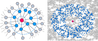
With a notion of concentric rings in $B_{\theta}(v,\rho)$, we can now define the pair correlation on a graph. Specifically, let $S=\operatorname{supp}(\boldsymbol{s})=\{s_{1},s_{2},\ldots,s_{m}\}$ be the support of the sampling pattern $\boldsymbol{s}$ and let $\left\|\boldsymbol{s}(B_{\theta}(s_{i},\rho))\right\|_{0}$ be the number of 1s of $\boldsymbol{s}$ on $B_{\theta}(s_{i},\rho)$, then the sample pair correlation function, $\mathcal{R}_{\boldsymbol{s}}(\rho)$, associated to $\boldsymbol{s}$ is defined by

$$\mathcal{R}_{\boldsymbol{s}}(\rho)=\frac{\frac{1}{m}\sum\limits_{i=1}^{m}\left\|\boldsymbol{s}(B_{\theta}(s_{i},\rho))\right\|_{0}}{\frac{1}{N}\sum\limits_{v\in V(G)}\|\boldsymbol{s}(B_{\theta}(v,\rho))\|_{0}}.$$ (11)

Notice that the numerator in (11) indicates the average number of 1s in $\boldsymbol{s}$ on a ring of width $\theta$ that is centered on a 1 of $\boldsymbol{s}$, while the denominator indicates the average number of 1s on the ring of the same width when it is centered at any arbitrary node. Now, the pair correlation for $q$ realizations $\boldsymbol{s}_{1},\ldots,\boldsymbol{s}_{q}$ of a random sampling pattern is defined as

$$\mathcal{R}(\rho)=\frac{1}{q}\sum_{r=1}^{q}\mathcal{R}_{\boldsymbol{s}_{r}}(\rho),$$ (12)

as the influence of a sampling point at node $v$ on all other nodes in the geodesic annular region $B_{\theta}(v,\rho)$. Notice that for the computation of eqn. (11) several values of $\theta$ can be considered, in this work the value of $\theta$ is the average of nonzero edge weights.

Note that a maxima of $\mathcal{R}(\rho)$ can be considered as an indication of the frequent occurrence of the inter-node distance, $\rho$, between nodes set to 1 whereas minima indicate a reduced occurrence. Since for random patterns the expected number of 1s in any annular ring is proportional to the number of nodes within the ring, we expect a pair correlation equal to 1 for all $\rho>0$ as illustrated in Fig. 1 (center).

Blue-noise, when applied to an image of constant gray-level $g$, spreads the minority pixels of the resulting binary image as homogeneously as possible such that the pixels are separated by an average distance, $\lambda_{b}$, referred to as the principal wavelength of blue-noise. These minority pixels are the pixels that are used to represent the properties of a region on a grayscale image, for instance in a dark region the minority pixels are labeled with 1 while in white regions the minority pixels are labeled with 0. Then, the value of $\lambda_{b}$ is defined as the radius of a round disc, surrounding a minority pixel, such that the ratio of the surface area of a minority pixel to the surface area of the disc is equal to the density of minority pixels, $d=g$ for $0<g\leq 1/2$ and $d=1-g$ for $1/2<g\leq 1$, which we can write as:

$$d=\frac{D_{x}D_{y}}{\lambda_{b}^{2}},$$ (13)

where $D_{x}$ and $D_{y}$ are the sampling periods (distance between samples) of the digital image in the $x$ and $y$ directions, respectively.

In order to extend the notion of principal wavelength to graphs, we need a notion of surface area as the expected number of graph nodes, $\mathbb{E}\{{\cal N}(\lambda)\}$, within a distance or path length, $\lambda$, of a given minority node. We expect the ratio of our single, minority node to all nodes within a path length, $\lambda_{b}$, to equal the density level according to:

$$d=\frac{1}{\mathbb{E}\{{\cal N}(\lambda_{b})\}}.$$ (14)

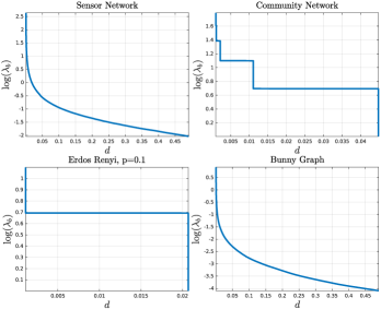
Being that $\mathbb{E}\{{\cal N}(\lambda_{b})\}$ is graph dependent, the graph blue-noise wavelength, $\lambda_{b}$, is likewise graph dependent and its characterization is still an open area of research [34, 35, 36]. In general, one can derive $\lambda_{b}$ versus $d$ experimentally as we have in Fig. 3 where we show the principal wavelength versus the density sampling $d$ for some commonly used graphs. We note that in the case of the sensor graph, $\lambda$ varies smoothly with $d=1/\mathbb{E}\{{\cal N}(\lambda_{b})\}$ while, in the case of the community graph, it varies with a piecewise constant behavior with respect to $d$.

Figure 3: Principal wavelength $\lambda_{b}$ versus the density of the sampling pattern for four different graphs traditionally considered in the literature.

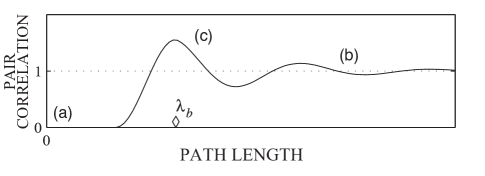
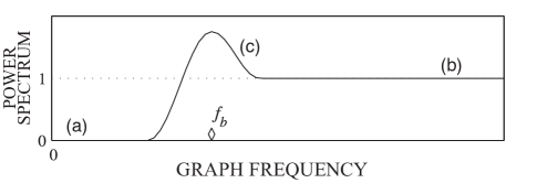
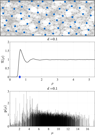
In light of the nature of graph blue-noise to isolate minority nodes, we can begin to characterize blue-noise graph signals in terms of the pair correlation, ${\cal R}(\rho)$, by noting that: (a) few or no neighboring minority nodes lie within a path length of $\rho<\lambda_{b}$; (b) for $\rho>\lambda_{b}$, the expected number of minority nodes per unit area tends to stabilize around a constant value; and (c) the average number of minority nodes within the path length, $\rho$, increases sharply nearly $\lambda_{b}$. The resulting pair correlation for blue-noise is, therefore, of the form in Fig. 4 (top), where ${\cal R}(\rho)$ shows: (a) a strong inhibition of minority nodes near $\rho=0$, (b) a decreasing correlation of minority nodes with increasing $\rho$ ($\lim_{\rho\rightarrow\infty}{\cal R}(\rho)=1$), and (c) a frequent occurrence of the inter-node distance $\lambda_{b}$, the principal wavelength, indicated by a series of peaks at integer multiples of $\lambda_{b}$. The principal wavelength is indicated in Fig. 4 (top) by a diamond located along the horizontal axis. Returning to the sample blue-noise signal of Fig. 5 (top), the resulting pair correlation of Fig. 5 (center) has a principal wavelength of $\lambda_{b}=0.56$ with a clearly visible peak of 1.55, meaning that nodes equal to 1 are $55\%$ more likely to occur at a distance of $\rho=0.56$ from an existing 1 than for the unconstrained probability of a node being equal to 1.

Figure 4: The ideal (top) pair correlation and (bottom) power spectra for blue-noise sampling patterns.

III-B Spectral Characteristics

Figure 5: Illustration of the spatial and spectral properties of (top) a blue-noise dither pattern on a Sensor Network graph with density, $d=0.1$, with (center) a pair correlation peak at the principal wavelength, $\lambda_{b}$, and (bottom) an approximately high frequency only power spectrum for frequencies, $\mu$.

Blue noise sampling patterns are characterized in traditional halftoning for a high frequency behavior [17]. In this section we state a connection between the spectral characteristics of a sampling pattern and its vertex domain characteristics, using the local properties of partitions of $V(G)$ that are measured by the isoperimetric constants of local induced subgraphs. In order to characterize the frequency content of a sampling pattern, a cost function is proposed. In particular, we propose a scalar measure of low-frequency energy, $R_{\boldsymbol{s}}$, in the signal $\boldsymbol{s}$, as the weighted sum of all Fourier coefficients’ energies:

$$R_{\boldsymbol{s}}=\frac{1}{\|\hat{\boldsymbol{s}}\|_{2}^{2}}\sum_{\ell=2}^{N}\frac{\hat{\boldsymbol{s}}^{2}(\ell)}{\mu_{\ell}}=\frac{1}{m}\sum_{\ell=2}^{N}\frac{\hat{\boldsymbol{s}}^{2}(\ell)}{\mu_{\ell}},$$ (15)

where $\hat{\boldsymbol{s}}$ is the graph Fourier transform of $\boldsymbol{s}$. $R_{\boldsymbol{s}}$ is coined as the redness of $\boldsymbol{s}$ as it measures low frequency spectral content.

In order to establish a connection between $R_{\boldsymbol{s}}$ and the vertex domain characteristics of a sampling pattern, it is important to consider the following theorems.

Theorem 4

For the graph $G=(V(G),E(G))$, let $\mathcal{P}=\left\{V(\Omega_{1}),V(\Omega_{2}),\ldots,V(\Omega_{|\mathcal{P}|})\right\}$ be a partition of $V(G)$, where $\Omega_{j}$ is the induced subgraph given by $V(\Omega_{j})$. Let $\delta_{j}$ be the isoperimetric dimension of $\Omega_{j}$. Then if

$$\delta_{1}=\delta_{2}=\ldots=\delta_{|\mathcal{P}|}=\delta$$ (16)

it follows that

$$\Lambda_{\mathcal{P}}>\min\left\{C_{\delta}\left(\frac{1}{vol(\Omega_{1})}\right)^{\frac{2}{\delta}},\ldots,C_{\delta}\left(\frac{1}{vol(\Omega_{|\mathcal{P}|})}\right)^{\frac{2}{\delta}}\right\}$$ (17)

where $C_{\delta}$ is a constant that depends on $\delta$.
Proof: See Appendix A

Theorem 4 indicates that when the graph has a local invariant isoperimetric dimension, the quality of a partition $\mathcal{P}$ for the representation of bandlimited signals, measured by $\Lambda_{\mathcal{P}}$, is defined by the set in $\mathcal{P}$ with the largest volume. The concept of isoperimetric dimension, originally defined on manifolds, provides a measure of how similar is the global behavior of a manifold with respect to a Euclidean space [37]. Similarly, in the case of graphs, the isoperimetric dimension indicates how close the behavior of a graph is with respect to regular grid-like graphs. For instance, the isoperimetric dimension of the $n-$dimensional regular grid is $n$ [37]. In the following theorem, we indicate when the right-hand side of eqn. (17) is maximized.

Figure 6: Partition of $V(G)$ for a graph $G$. Each color indicates the subgraph $\Omega_{j}$ induced by $V(\Omega_{j})$. Illustration shows how a sampling pattern can be built from the partition selecting the sampling nodes on the set $S$, whose nodes are indicated in black color. Notice that the sampling pattern indicated satisfies eqn. (19) and eqn. (20).

Theorem 5

Under the conditions stated in Theorem 4 and for a fixed value of $|\mathcal{P}|$, the partition that maximizes the right hand side of eqn. (17) satisfies that

$$vol(\Omega_{i})=vol(\Omega_{j})\quad\forall i,j.$$ (18)

Proof: See Appendix B

Under the conditions stated in Theorem 4, Theorem 5 provides the characteristics of the partition that will maximize the bandwidth of signals that can be represented in a unique way via their average values on the elements of the partition.

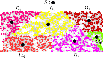
Now, it is important to notice that for any partition $\mathcal{P}=\left\{V(\Omega_{1}),V(\Omega_{2}),\ldots,V(\Omega_{|\mathcal{P}|})\right\}$, it is possible to build a sampling pattern, locating one sampling node per partition element (see Fig. 6). In the following theorem, we show that the spectral characteristics of such sampling patterns, measured by $R_{\boldsymbol{s}}$, are bounded by the local characteristics of the elements in $\mathcal{P}$.

Theorem 6

Let $\mathcal{P}=\left\{V(\Omega_{1}),V(\Omega_{2}),\ldots,V(\Omega_{|\mathcal{P}|})\right\}$ a partition of $V(G)$ and let $\boldsymbol{s}\in\{0,1\}^{N}$ a sampling pattern chosen according to

$$\|\boldsymbol{s}(V(\Omega_{j}))\|_{0}=1\quad\forall j$$ (19)

$$\text{If}~{}\boldsymbol{s}(v)=1,~{}\text{then}~{}\boldsymbol{s}(u)=0\quad\forall u\sim v$$ (20)

then

$$R_{\boldsymbol{s}}\leq\frac{(\mu_{2}+\mu_{N})^{2}(1-|\mathcal{P}|/N)^{2}}{4\mu_{2}\mu_{N}\min\limits_{j}\left\{\frac{C_{\delta_{j}}}{vol(\Omega_{j})^{2/\delta_{j}}}\right\}}.$$ (21)

If in addition, $\delta=\delta_{1}=\ldots=\delta_{|\mathcal{P}|}$ and $vol(\Omega)=vol(\Omega_{1})=\ldots=vol(\Omega_{|\mathcal{P}|})$, then

$$R_{\boldsymbol{s}}\leq\frac{(\mu_{2}+\mu_{N})^{2}(1-|\mathcal{P}|/N)^{2}vol(\Omega)^{\frac{2}{\delta}}}{4C_{\delta}\mu_{2}\mu_{N}}.$$ (22)

Proof: See Appendix C

In order to discuss the meaning and implications of Theorem 6, it is important to mention that eqn. (19) and eqn. (20) imply that there is one sampling node per element of the partition with $\|\boldsymbol{s}\|_{0}=|\mathcal{P}|$, and that there is a minimum interdistance between the sampling nodes in $\boldsymbol{s}$ (see Fig. 6). In particular, eqn. (20) assures that the sampling points in $\boldsymbol{s}$ are far from the boundaries of the elements of the partition.

Notice that eqn. (21) presents a general upper bound for the redness of an arbitrary sampling pattern subject to eqn. (19) and eqn. (20). Meanwhile, eqn. (22) provides a tighter bound that is connected with blue-noise sampling patterns as a consequence of having the elements in the partition with the same volume and the same isoperimetric dimension. In this second case, we see that as the size of the partition, $\mathcal{P}$, increases (and therefore the number of sampling nodes in $\boldsymbol{s}$) $vol(\Omega)$ decreases and so it is the value $R_{\boldsymbol{s}}$, making clear the connection between a uniform vertex spreading of the sampling nodes in $\boldsymbol{s}$ and a low redness. As a consequence, a behavior like the one depicted in Fig. 5 (bottom) is expected. It is important to emphasize that this statement is connected to Theorems 4 and 5, where the characteristics of good partitions for the representation of bandlimited signals is stated. In the case of the traditional halftoning scenario where the problem is modeled on a 2-dimensional grid, the conditions of Theorems 6, 5 and 4 hold and a typical response like the one shown in Fig. 4 (bottom) is obtained.

Theorem 6 also implies that there is an upper limit about the number of elements in the partition $\mathcal{P}$ that can be considered, and with that, it comes a limitation in the number of sampling nodes for which these inequalities hold. In particular, for very large values of $|\mathcal{P}|$, eqn. (19) and eqn. (20) cannot be satisfied. We point out that this does not diminish the quality of the sampling patterns, but instead points out that the relationship between the spectral domain and the vertex domain is not guaranteed to be governed by eqn. (21).

III-B1 Spectral Metrics

It is also possible to characterize the spectral properties of binary dither patterns on a graph where we extend the idea of periodograms to graphs such that the GFTs of $q$ realizations of $\boldsymbol{x}$, i.e. $\boldsymbol{x}_{1},\boldsymbol{x}_{2},\ldots,\boldsymbol{x}_{q}$, are averaged together to form the power spectrum:

$$\mathbf{p}(\ell)=\frac{N}{q}\sum_{i=1}^{q}\frac{\hat{\boldsymbol{x}}_{i}(\ell)^{2}}{\|\hat{\boldsymbol{x}}_{i}\|_{2}^{2}}\quad\ell=2,\ldots,N.$$ (23)

Notice that the $\ell^{th}$ component of $\mathbf{p}$ is associated with the $\ell^{th}$ eigenvalue $\mu_{\ell}$. Like its binary halftone counterpart, the GFT of a white-noise sampling pattern is expected to be flat for all $\mu_{k}$s, and to visualize this power spectra, Fig. 1 (bottom) shows an estimate of the power spectra for 100 unique white-noise dither patterns generated on the 2000-node Sensor Network graph with pattern density $d=0.1$.

III-C Blue-noise Sampling Sets

In the following corollary we state how from a blue-noise sampling pattern a good partition in the sense of Theorem 3 can be obtained.

Corollary 7

Let $\boldsymbol{s}$ be a blue-noise sampling pattern obtained according to Definition 1, with $\|\boldsymbol{s}\|_{0}=m$ and $\operatorname{supp}(\boldsymbol{s})=\{s_{1},s_{2},\ldots,s_{m}\}$. Let $B(s_{j},\lambda)$ be as specified in Definition 1. Then, there exists a partition $\mathcal{P}=\left\{V(\Omega_{1}),V(\Omega_{2}),\ldots,V(\Omega_{|\mathcal{P}|})\right\}$ of $V(G)$ such that

$$u\in V(\Omega_{j})\Leftrightarrow u\in B(s_{j},\lambda),u\notin B(s_{i},\lambda)~{}\forall~{}i\neq j$$ (24)

and the elements in the intersection between the sets $B(s_{i},\lambda)$ are distributed on the $V(\Omega_{i})$ such that the quantity $\sum_{i\neq j}\left|vol(\Omega_{i})-vol(\Omega_{j})\right|$ is minimized. Additionally if $\Lambda_{\mathcal{P}}>(1+1/\alpha)\omega$, $\alpha>0$ any $\boldsymbol{x}\in PW_{\omega}(G)$ can be uniquely determined from its values at $\{s_{1},s_{2},\ldots,s_{m}\}$ always that $\boldsymbol{x}(s_{j})=\boldsymbol{x}^{\mathsf{T}}(\boldsymbol{\xi}_{j}\circ\boldsymbol{\xi}_{j})~{}\quad\forall j$.

Proof: See Appendix E.

This corollary indicates that given a sampling pattern whose sampling points are located as far as possible from each other, it is possible to build a partition from which a unique representation of a set of bandlimited signals is possible. Additonally, if the conditions of Theorem 4 are satisfied, then the partitions obtained are the ones that maximize the value of $\Lambda_{\mathcal{P}}$.

Theorem 1 tells us that when a fixed value of the bandwidth $\omega$ is considered and a signal has to be sampled taking $m$ samples, it is necessary to look for the set of nodes, $S$, such that $S^{c}$ is a $\Lambda_{S^{c}}$-removable set with $\omega<\Lambda_{S^{c}}$. Finding the subset of $m$ nodes with the maximum $\Lambda_{S^{c}}$ would, therefore, give the best sampling set. On the other hand, if a signal has to be sampled taking a number of $m$ samples, choosing a set of nodes $S$ with the maximum value of $\Lambda_{S^{c}}$ will extend the class of signals, $PW_{\omega}(G)$, that can be sampled and represented in a unique way with $m$ samples.

Now if one can show that minimizing the redness in a sampling signal promotes high values of $\Lambda_{S^{c}}$, one could argue blue-noise was a desirable attribute for efficient sampling. The following theorem establishes this relationship:

Theorem 8

Let $\boldsymbol{s}:V(G)\longrightarrow\{0,1\}$ be a sampling pattern with $\boldsymbol{s}({S})=1$, $\boldsymbol{s}({S^{c}})=0$ for $S\subset V(G)$ and $|S|=\|\boldsymbol{s}\|_{0}=m$, then the $\Lambda_{S^{c}}-$constant of the set $S^{c}$ satisfies

$$\Lambda_{S^{c}}>C_{\delta}\left(\frac{R_{\boldsymbol{s}}}{vol(G)R_{\boldsymbol{s}}-m\left(1-\frac{m}{N}\right)^{2}}\right)^{\frac{2}{\delta}}$$ (25)

where $R_{\boldsymbol{s}}$ is the redness in $\boldsymbol{s}$ from eqn. (15); $\delta$ is the isoperimetric dimension of $G$ [20, 38]; and $C_{\delta}$ a constant that depends only on $\delta$.
Proof: See Appendix F.

To summarize, Theorem 8 tells us that the best sampling set, $S$, is the one for which the value of $\Lambda_{S^{c}}$ is a maximum; therefore while blue-noise sampling patterns (which minimize $R_{\boldsymbol{s}}$) are not necessarily the best sampling sets, they are good sampling sets. Notice that eqn. (25) is well defined as $vol(G)R_{\boldsymbol{s}}-m\left(1-\frac{m}{N}\right)^{2}>0$, which is tight when $S^{c}\cup bS^{c}=V(G)$ where $bS^{c}$ is the boundary of $S^{c}$. This criteria can be satisfied making the nodes in $S$ as spread apart as possible in the graph, which is reasonable as a sampling set where all the nodes are too concentrated in one area could lead to poor reconstructions of signals that exhibit fast changes in the sparsely sampled areas left elsewhere.

As an approach to reinforce the benefits of blue-noise sampling sets, we can use the quantities introduced in Theorem 2 to show how blue-noise promotes those sampling sets that maximize the bandwidth of the signals that can be represented in a unique way on a given sampling set as indicated in the following theorem:

Theorem 9

Let $\boldsymbol{s}:V(G)\longrightarrow\{0,1\}$ with $\boldsymbol{s}({S})=1$, $\boldsymbol{s}({S^{c}})=0$, $S\subset V(G)$. If $K_{S}>0$, then

$$K_{S}\geq\left(\frac{m\left(1-\frac{m}{N}\right)^{2}}{R_{\boldsymbol{s}}}-\gamma\right)^{1/2}$$ (26)

where $\gamma=\max_{S,v^{{}^{\prime}},v}\left(\sum_{v\in S^{c}\setminus v^{{}^{\prime}}}w_{S}(v)^{2}\right),$ and $R_{\boldsymbol{s}}$ is, again, the redness in $\boldsymbol{s}$ from eqn. (15).
Proof: See Appendix G.

Figure 7: Void and cluster blue-noise sampling patterns for different intensities $d$ for a sensor network graph. First row: Localization on the graph of the nodes selected in a blue-noise sampling pattern. Second row: The pair correlation function $\mathcal{R}(\rho)$ for the sampling patterns indicating with a diamond marker the value of $\lambda_{b}$. Third row: Power spectral density for the different blue-noise sampling patterns.

Theorem 9 indicates that lowering the redness of the sampling pattern raises the minimum possible value of $K_{S}$ and, therefore, extends the set of signals, $PW_{\omega}(G)$, that can be represented in a unique way on a given sampling set. Therefore, again the blue-noise sampling patterns that are characterized by small values of $R_{\boldsymbol{s}}$ represent a better option than arbitrary random sampling, which leads to large values of $R_{\boldsymbol{s}}$.

It is important to point out that, under the conditions stated in Theorem 4, Theorems 8 and 9 show that the reduction of the redness is a desirable attribute for any sampling pattern, which is something that can be considered with other sampling approaches. Additionally, the tightness of the inequalities depends on the graph structure which makes these results stronger in some families of graphs.

III-D Stability and blue-noise sampling Sets

The selection of a sampling set, $S$, is not only associated to a possible unique representation of a signal but also to the stability of its reconstruction when the samples are corrupted by noise, or when the signal considered is not exactly bandlimited. This stability can be measured considering the condition of the matrix $\mathbf{U}_{k}(S,:)$, which is the matrix obtained by sampling $\mathbf{U}_{k}$ on the rows indicated by $S$ [24]. Several cost functions can be formulated in terms of the condition of $\mathbf{U}_{k}(S,:)$, such that their minimum or maximum values are given by the sampling set that provides the best condition [24].

The measures of stability provided in [24] can be equivalently obtained from a formal general definition of stability for sampling sets in arbitrary spaces [39]. In particular, recalling the definition of stability presented in [39] for general sampling schemes, we can say that $PW_{\omega}(G)$ posses a stable sampling expansion or reconstruction on $S\subset V(G)$ if there exists $C\geq 1$ such that $\|\boldsymbol{x}(S^{c})\|_{2}^{2}\leq(C-1)\|\boldsymbol{x}(S)\|_{2}^{2}\quad\forall\boldsymbol{x}\in PW_{\omega}(G)$. The value of $C$ provides a measure of stability associated to $S$; the larger the value of $C$ the less stability we have. In the following theorem we provide an estimate of $C-1$ in terms of $\Lambda_{S^{c}}$.

Theorem 10

Let $\boldsymbol{x}\in PW_{\omega}(G)$. Then, if $\Lambda_{S^{c}}>\tilde{\omega}$, it follows that

$$\|\boldsymbol{x}(S^{c})\|_{2}^{2}\leq\frac{\left(\frac{\tilde{\omega}^{r}}{\Lambda_{S^{c}}}\right)^{2}}{1-\left(\frac{\tilde{\omega}^{r}}{\Lambda_{S^{c}}}\right)^{2}}\|\boldsymbol{x}(S)\|_{2}^{2}\quad r\in\mathbb{R}_{+}$$ (27)

where $\tilde{\omega}$ is the bandwidth of $\boldsymbol{x}_{1}$, $\boldsymbol{x}_{1}(S^{c})=\boldsymbol{x}(S^{c})$ and $\boldsymbol{x}_{1}(S)=0$.
Proof: See Appendix H

From this theorem, it is important to point out that finding the sampling set $S$ for which $\Lambda_{S^{c}}$ is maximum not only provides a unique representation of a bandlimited signal, but also provides the sampling set in which the highest stability is achieved. This result is consistent with the findings in [24].

As it was stated in Theorem 8, patterns with a low redness promote large values of $\Lambda_{S^{c}}$, therefore blue-noise sampling patterns not only promote uniqueness of the representation but also stability in the reconstruction.

III-E Connection with other works

The implications and properties of spreading the sampling points as far as possible from each other on non Euclidean domains were formally established by Pesenson in [40] considering functions on compact Riemmanian manifolds. In [41, 42, 43] the concept of blue-noise was used for the sampling of surfaces embeded in $\mathbb{R}^{3}$ for applications in computer graphics. This last result can be considered an application of the results in [40] for two-dimensional manifolds embedded in $\mathbb{R}^{3}$. It is important to point out that the results in [41, 42, 43] rely on the mapping that can be established between the surface and a subset of the 2-dimensional Euclidean domain, but they do not offer any insight of how to deal with the problem in higher dimensions. In [44] a method is proposed for the optimal location of sensors in Euclidean spaces. Exploiting the concepts of entropy, mutual information and Gaussian processes (GPs), the problem of selecting a subset of sensors among a predefined set of discrete positions, defined on a grid of an $n-$dimensional Euclidean space, is addressed. To deal with a large number of possible sensor locations some relaxations based on lazy evaluations and local structure of (GPs) are used.

In a different context, and before the emergence of graph signal processing, functions defined on the vertices of a graph have been considered under the concept of fitness landscapes [23, 45], which were introduced as a tool for the study of molecular evolution. In this context, the length of the autocorrelation function has been useful for the analysis of a landscape. In particular, the correlation length of a landscape, $\boldsymbol{x}$, on a $K$-regular graph is given by [45]

$$\ell_{\boldsymbol{x}}=\frac{K}{\|\hat{\boldsymbol{x}}\|_{2}^{2}}\sum_{\ell=2}^{N}\frac{\hat{\boldsymbol{x}}(\ell)^{2}}{\mu_{\ell}}.$$ (28)

The values of eqn. (28) provide an indication about how correlated are a given set of samples of the landscape obtained using a random walk. As can be observed in eqn. (28) this is proportional to the redness of $\boldsymbol{x}$. In this context, it is possible to conceive blue-noise sampling patterns on graphs as landscapes with a low length correlation.

IV Generating Blue-Noise Sampling Sets

Figure 8: Void and cluster blue-noise sampling patterns for different intensities $d$ for a community graph. First row: Localization on the graph of the nodes selected in a blue-noise sampling pattern. Second row: The pair correlation function $\mathcal{R}(\rho)$ for the sampling patterns indicating with a diamond marker the value of $\lambda_{b}$. Third row: Power spectral density for the different blue-noise sampling patterns.

Figure 9: Illustration of the redness, $R_{\boldsymbol{s}}=\frac{1}{m}\sum_{\ell=2}^{N}\frac{\hat{\boldsymbol{s}}(\ell)^{2}}{\mu_{\ell}}$, of the void and cluster blue-noise sampling patterns on a sensor network with $N=2000$ nodes, considering different densities.

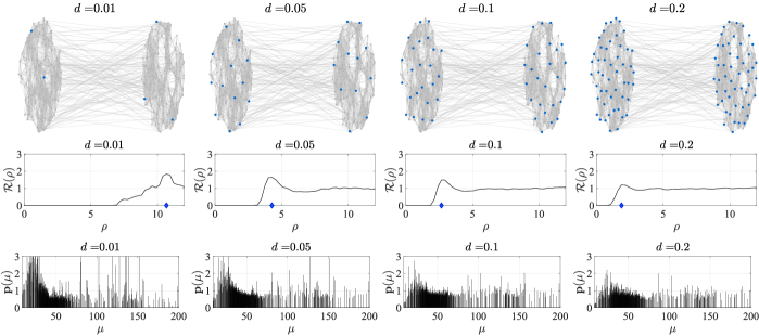
Given that blue-noise graph signal sampling promotes the finding of good sampling sets, it is natural to ask how such sampling patterns can be generated. An algorithm that has been particularly successful in digital halftoning and that intuitively translates to graphs is the Void-And-Cluster (VAC) algorithm, introduced by Ulichney [18]. VAC allows for the construction of artifact-free homogeneous dithering patterns by iteratively measuring the concentration of minority pixels in a binary halftone image, using a gaussian low-pass filter, and swapping the minority pixels in the area of highest concentration with the non-minority pixel in the area of lowest concentration. The adaptation of this algorithm to sampling signals on graphs consists roughly speaking of the sequential computation of distances between sampling points in such a way that points with short geodesic distances between them are relocated trying to put them far from each other.

In order to exploit the above principle for the selection of sampling nodes on a graph, a Gaussian kernel $\displaystyle\mathbf{K}(u,v)=exp(-\mathbf{\Gamma}(u,v)^{2}/\sigma)$ is evaluated on the set of geodesic distances, $\mathbf{\Gamma}$. This provides a new set of distances that can be tuned according to the parameter, $\sigma$, where a small value of $\mathbf{\Gamma}(u,v)$ leads to a value of $\mathbf{K}(u,v)$ that is close to unity while a large value of $\mathbf{\Gamma}(u,v)$ leads to a value of $\mathbf{K}(u,v)$ close to zero. As a measure of how homogeneously distributed the sampling points are, the sum of all distances from one node to the others via the kernel $\mathbf{K}$ is calculated as $\mathbf{c}=\mathbf{K}\mathbf{1}_{N\times 1}$. With this, an initial sampling pattern is generated selecting the $m$ components of $\mathbf{c}$ at random, where $m=dN$ is the number of 1’s in the sampling pattern with density $d$.

Algorithm 1 Void and cluster algorithm for graphs

0:  $m$: number of samples, $\sigma$, NumIter.

0:  $\boldsymbol{s}$: sampling pattern Initialisation : $\boldsymbol{s}=\mathbf{0}$, IndA=-1, IndB=-1.

  Calculate $\displaystyle\mathbf{K}(i,j)=e^{-\frac{\mathbf{\Gamma}(i,j)^{2}}{\sigma}}$ for all $1\leq i,j\leq N$.

2:  $\mathbf{c}=\mathbf{\mathbf{K}}\mathbf{1}_{N\times 1}$.

  Get $\mathcal{M}$ as $m$ nodes selected at random.

4:  $\boldsymbol{s}(\mathcal{M})=1$.

  for $r=1:1:\texttt{NumIter}$ do

6:     $\mathbf{c}(\operatorname{supp}(\boldsymbol{s}))=\sum\mathbf{K}(\operatorname{supp}(\boldsymbol{s}),\operatorname{supp}(\boldsymbol{s}))$.

     $\mathbf{c}(\operatorname{supp}(\boldsymbol{s})^{c})=\sum\mathbf{K}(\operatorname{supp}(\boldsymbol{s}),\operatorname{supp}(\boldsymbol{s})^{c})-\tau$.

8:     $\boldsymbol{s}\left(\arg\max_{i}\{\mathbf{c}(i)\}\right)=0$.

     $\boldsymbol{s}\left(\arg\min_{i}\{\mathbf{c}(i)\}\right)=1$.

10:     if IndA=$\arg\max_{i}\{\mathbf{c}(i)\}$ and IndB=$\arg\min_{i}\{\mathbf{c}(i)\}$ then

        break

12:     else

        IndA=$\arg\min_{i}\{\mathbf{c}(i)\}$.

14:        IndB=$\arg\max_{i}\{\mathbf{c}(i)\}$.

     end if

16:  end for

  return  $\boldsymbol{s}$

The components of $\mathbf{c}$ whose index is given by the location of the 1’s in $\boldsymbol{s}$, are then updated to be $\mathbf{c}(\operatorname{supp}(\boldsymbol{s}))=\sum\mathbf{K}(\operatorname{supp}(\boldsymbol{s}),\operatorname{supp}(\boldsymbol{s}))$, where $\sum\mathbf{K}(A,B)$ is defined by

$$\sum\mathbf{K}(A,B)=\sum_{a_{i},b_{j}}\mathbf{K}(a_{i},b_{j})\quad a_{i}\in A,b_{j}\subset{B}.$$ (29)

The remaining components of $\mathbf{c}$ are updated according to $\mathbf{c}(\operatorname{supp}(\boldsymbol{s})^{c})=\sum\mathbf{K}(\operatorname{supp}(\boldsymbol{s}),\operatorname{supp}(\boldsymbol{s})^{c})-\tau$, where $\tau$ is selected as a large scalar value. With this update the distances between sampling points in the pattern are represented as positive quantities without adding the distances to other nodes. The distance between $\operatorname{supp}(\boldsymbol{s})$ and $\operatorname{supp}(\boldsymbol{s})^{c}$ is then represented with a negative value. Now the index of the component of $\mathbf{c}$ with the highest value will indicate the sampling point that is closest to the other sampling points, and then the value of $\boldsymbol{s}$ at that index is forced to be $0$ whereas in the index where $\mathbf{c}$ is minimum, $\boldsymbol{s}$ is forced to be 1. Notice that the role of $\tau$ is to make sure that always $\mathbf{c}(\operatorname{supp}(\boldsymbol{s})^{c})<0$ and a variety of values for $\tau$ would serve this purpose. Taking into account that $\sum\mathbf{K}(\operatorname{supp}(\boldsymbol{s}),\operatorname{supp}(\boldsymbol{s})^{c})\leq N$, it is possible to select $\tau$ as any value such that $\tau>N$.

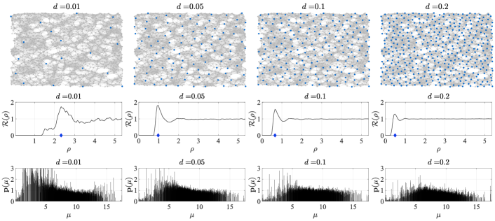
Repeating the above process iteratively, it is possible to achieve a sampling pattern with no clusters of 1s that exhibits a homogeneous distribution on $V(G)$. The details of the VAC algorithm can be appreciated in Algorithm 1 with example sampling patterns using VAC depicted in Fig. 7 for the Sensor Network graph and in Fig. 8 for a community graph. From observation, one can see a clear distinction with respect to random sampling when it comes to the nodes distribution of the sampling set. The spatial and spectral blue-noise-like behavior is obtained as a byproduct of the algorithm.

At this point, we note that the value of $\sigma$ in the kernel $exp(-\mathbf{\Gamma}(u,v)^{2}/\sigma)$ plays a critical role in VAC as it defines which sampling nodes are close enough to another one in order to produce a relocation of the $1$’s in the sampling pattern. Taking into account the definition of $\lambda_{b}$ presented in previous sections, it is possible to establish a natural connection between $\sigma$ and $\lambda_{b}$. In order to do so, we note that if the blue-noise sampling pattern is ideally distributed on the set of nodes, $V(G)$, then when $u$ and $v$ are sampling nodes it follows that $exp(-\mathbf{\Gamma}(u,v)^{2}/\sigma)\approx 0$ if $\mathbf{\Gamma}(u,v)\geq\lambda_{b}$. This criteria is considered to be satisfied when $\sigma=\lambda_{b}^{2}/ln(10)$, i.e selecting $\sigma$ in this way the exponential reaches a value of $0.1$ when $\mathbf{\Gamma}(u,v)=\lambda_{b}$. The number of iterations NumIter is selected as a multiple of $N$. In the numerical experiments performed, we have found that choosing $\texttt{NumIter}=N$ is enough for the algorithm to reach a stationary behavior.

Figure 10: Averaged MSE using the reconstruction stated in (4) vs the sampling rate considering the reconstruction of 100 different signals from its samples using several sampling schemes and considering several graphs: (a) The graph $G_{1}$ and the signal model SM1. (b) The graph $G_{2}$ and the signal model SM1. (c) The graph $G_{3}$ and the signal model SM1. (d) The graph $G_{1}$ and the signal model SM2. (e) The graph $G_{2}$ and the signal model SM2. (f) The graph $G_{3}$ and the signal model SM2.

Figure 11: Averaged MSE using the reconstruction method proposed in [26] vs the sampling rate considering the reconstruction of 100 different signals from its samples using several sampling schemes and considering several graphs: (a) The graph $G_{1}$ and the signal model SM1. (b) The graph $G_{2}$ and the signal model SM1. (c) The graph $G_{3}$ and the signal model SM1. (d) The graph $G_{1}$ and the signal model SM2. (e) The graph $G_{2}$ and the signal model SM2. (f) The graph $G_{3}$ and the signal model SM2.

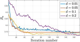
As indicated in Fig. 9, there is a clear reduction of the redness of the patterns as they get better distributed on the nodes of the graph. It is important to mention that the number of iterations required for the redness to drop to its minimum value increases as the value of $d$ increases. This is related with the fact that, as $d$ is reduced, there are more possibilities for the relocation of the $1$’s in the sampling pattern.

V Experiments

In order to evaluate the benefits of blue-noise sampling, a set of numerical experiments is performed comparing the obtained results against state of the art techniques. The simulations are performed considering different graphs and signal models. The experiment is described by the following steps:

• For each graph model, a set of 100 signals is generated according to the specific signal models selected.

• Each signal is sampled by means of different sampling schemes.

• The signal reconstructed from the samples is compared to the original one, and its mean squared error (MSE) is calculated.

• The values of the MSE are averaged over 100.

The schemes of sampling considered for the experiment are the following:

• Blue noise sampling by void and cluster.

• Sampling scheme proposed by Chen et. al. [14].

• Sampling scheme proposed by Anis et. al. [24].

• Sampling scheme proposed by Tsitsvero et al. [28].

The signal models are:

• Signal model 1 (SM1): A random signal of bandwidth $k=50$, where the Fourier coefficients are generated from the Gaussian distribution $\mathcal{N}(1,0.5^{2})$. The samples captured are contaminated with additive Gaussian noise such that the Signal to Noise Ratio is $SNR=20$dB.

• Signal model 2 (SM2): A random signal with Fourier coefficients generated from the Gaussian distribution $\mathcal{N}(1,0.5^{2})$. This signal is modulated on the spectral axes by $h(\mu)$, where

  $$h(\mu)=\left\{\begin{array}[]{ccc}1&\text{If}&\mu\leq\mu_{50}\\ e^{-4(\mu-\mu_{50})}&\text{If}&\mu>\mu_{50}\\ \end{array}\right.$$ (30)

The graphs considered in the simulations are different from each other in their nature and represent typical graphs that can be found in different scenarios and applications. The graph models used are:

• Graph $G_{1}$: A random sensor network with $N=1000$ nodes. The weights in the graph are given by the Euclidean distance between points. The maximum number of neighbors for each node is 6.

• Graph $G_{2}$: A community graph with $N=1000$ nodes, 16 communities generated using the GSP toolbox [46].

• Graph $G_{3}$: A Barabási-Albert random network [4] with $N=1000$ nodes.

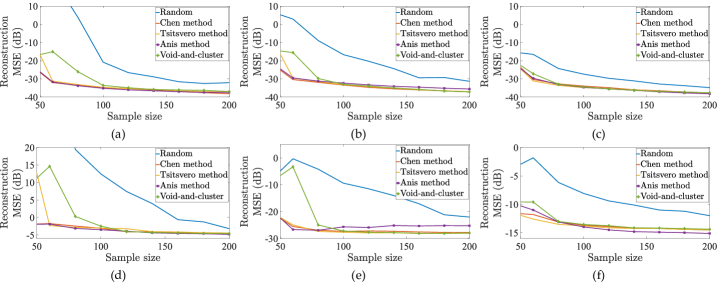
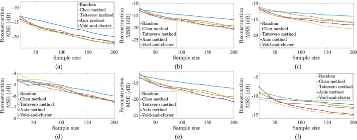
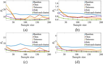
The reconstructions are performed by means of eqn. (4) and by the interpolation splines proposed in [26] and implemented in [46]. In Figs. 10 and 11, the performance of different algorithms can be appreciated including VAC sampling. Notice that the decay rate of the error curves show consistently the benefits of blue-noise sampling. The results obtained using VAC are close to the ones obtained in [24]. Additonally, in Fig. 12, the redness of the sampling patterns obtained by different techniques are presented considering different graphs. It is possible to see how low redness is a characteristic attribute of good sampling patterns.

Figure 12: Illustration of the redness $R_{\boldsymbol{s}}=\frac{1}{m}\sum_{\ell=2}^{N}\frac{\hat{\boldsymbol{s}}(\ell)^{2}}{\mu_{\ell}}$ for the sampling patterns generated by different sampling approaches on different graphs. (a) Swiss roll graph; (b) Sensor network graph; (c) Sphere graph; (d) Bunny graph.

VI Conclusion

Blue-noise sampling on graphs is defined based on the traditional blue-noise model associated with digital halftones. The properties and benefits of blue-noise sampling on graphs are linked with theoretical results related to uniqueness sets in sampling, showing why blue-noise patterns promote good sampling sets. We also extended void and cluster, a popular halftoning scheme to generating blue-noise sampling sets on graphs. Numerical tests on different graphs corroborate the good qualities of sampling with blue-noise. We specified conditions under which the traditional relationship between vertex-domain spreading and frequency behavior is preserved. We further note that the results obtained in this work can be extended for specific families of graphs. The delimitation of the properties for the graphs under consideration could lead to sharper bounds and could allow the definition of other quantities extensively used in halftoning, like the principal frequency.

An overlooked benefit to blue-noise sampling is the wealth of computationally efficient algorithms used in digital halftones that can be extended to graph sampling without spectral estimation, namely error-diffusion where the produced halftone patterns conform to the local spectral content of the image to optimally preserve salient features like edges, gradients, flood fills, etc. Also, a very valuable attribute of error-diffusion that is not widely recognized outside the halftoning community is that error-diffusion can be trained to produce arbitrary spectral profiles (blue-noise, green-noise, etc) and even designed to match the dither patterns produced by other means, including ones with high computational complexity [17, 47]. For graph signal sampling, this opens up the possibility of error-diffusion algorithms trained to mimic sampling algorithms based on spectral estimation and vertex-domain characteristics. We consider that an interesting topic for future research would be the analysis and implications of blue-noise sampling on graphs for signals that are bandlimited but not necessarily low pass [48, 49]. This could provide a generalization of the results that were stated in this work.

It is important to point out that blue-noise sampling promotes large values of $\Lambda_{S^{c}}$, but there is not a guarantee about reaching the maximum value of $\Lambda_{S^{c}}$. For this reason the stability is affected when the value of $\Lambda_{S^{c}}$ is not large enough, which also happens when $m$ is not large enough. This aspect is something that can be improved in future works adding additional constraints to the method used to generate blue-noise sampling patterns.

Appendix A Proof of Theorem 4

Proof.

As stated in [38] (page 168), by means of Sobolev inequalities, it is possible to state that

$$\mu_{1,j}\geq C_{\delta_{j}}\frac{1}{vol(\Omega_{j})^{\frac{2}{\delta_{j}}}}$$ (31)

where $\delta_{j}$ is the isoperimetric dimension of $\Omega_{j}$ and $C_{\delta_{j}}$ is a constant that depends only on $\delta_{j}$. Taking into account the definition of $\Lambda_{\mathcal{P}}$ in Theorem 3 we do have that

$$\Lambda_{\mathcal{P}}>\min\left\{\frac{C_{\delta_{1}}}{vol(\Omega_{1})^{\frac{2}{\delta_{1}}}},\ldots,\frac{C_{\delta_{|\mathcal{P}|}}}{vol(\Omega_{|\mathcal{P}|})^{\frac{2}{\delta_{|\mathcal{P}|}}}}\right\}$$

if $\delta_{1}=\delta_{2}=\ldots=\delta_{|\mathcal{P}|}=\delta$, then it follows that

$$\Lambda_{\mathcal{P}}>\min\left\{\frac{C_{\delta}}{vol(\Omega_{1})^{\frac{2}{\delta}}},\ldots,\frac{C_{\delta}}{vol(\Omega_{|\mathcal{P}|})^{\frac{2}{\delta}}}\right\}$$

∎

Appendix B Proof of Theorem 5

Proof.

In order to simplify notation lets represent $x_{i}=vol(\Omega_{i})^{2/\delta}/C_{\delta}$ and lets consider the optimization problem

$$\underset{\{x_{1},x_{2},\ldots,x_{|\mathcal{P}|}\}}{\text{maximize}} \min\{1/x_{1},1/x_{2},\ldots,1/x_{|\mathcal{P}|}\}$$ (32)

subject to $$\sum_{i=1}^{|\mathcal{P}|}x_{i}=c_{1},\quad x_{i}>0~{}\forall i$$

where $c_{1}$ is a constant. Now, taking into account that

$$\min\{1/x_{1},1/x_{2},\ldots,1/x_{|\mathcal{P}|}\}\sum_{i=1}^{|\mathcal{P}|}x_{i}\leq\sum_{i=1}^{|\mathcal{P}|}x_{i}\frac{1}{x_{i}}=|\mathcal{P}|$$

$$\min\{1/x_{1},1/x_{2},\ldots,1/x_{|\mathcal{P}|}\}\leq|\mathcal{P}|/c_{1}.$$

Then, the maximum value of the objective function in eqn. (32) is $|\mathcal{P}|/c_{1}$. Let $(x_{1}^{*},x_{2}^{*},\ldots,x_{|\mathcal{P}|}^{*})$ the optimal solution of (32), then it follows that $|\mathcal{P}|/c_{1}\leq 1/x_{i}^{*}$. Lets assume there exists a subset of indexes $\{j_{1},j_{2},\ldots,j_{q}\}\subset\{1,\ldots,|\mathcal{P}|\}$ such that $|\mathcal{P}|/c_{1}<1/x_{j_{r}}^{*}$ which implies $x_{j_{r}}^{*}<c_{1}/|\mathcal{P}|$. Then it follows that

$$\sum_{i=1}^{|\mathcal{P}|}x_{i}=\left(|\mathcal{P}|-q\right)\frac{c_{1}}{|\mathcal{P}|}+\sum_{j_{r}}x_{j_{r}}<c_{1}$$ (33)

which is a contradiction. Therefore $x_{i}^{*}=c_{1}/|\mathcal{P}|$ which implies $x_{1}^{*}=x_{2}^{*}=\ldots=x_{|\mathcal{P}|}^{*}$. ∎

Appendix C Proof of Theorem 6

Proof.

Let $\boldsymbol{s}\in\{0,1\}^{N}$ selected according to (19) and (20), then it follows that $\boldsymbol{s}^{\mathsf{T}}\mathbf{L}\boldsymbol{s}=\sum_{j=1}^{|\mathcal{P}|}\boldsymbol{s}(V(\Omega_{j}))^{\mathsf{T}}\mathbf{L}_{\Omega_{j}}\boldsymbol{s}(V(\Omega_{j})).$ Additionally, directly from the definition of $\mu_{1,j}$ and using the Raleyigth coefficient we have $\mu_{1,j}\leq\boldsymbol{s}(V(\Omega_{j}))^{\mathsf{T}}\mathbf{L}_{\Omega_{j}}\boldsymbol{s}(V(\Omega_{j}))$. Therefore

$$\sum_{j=1}^{|\mathcal{P}|}\mu_{1,j}\leq\sum_{j=1}^{|\mathcal{P}|}\boldsymbol{s}(V(\Omega_{j}))^{\mathsf{T}}\mathbf{L}_{\Omega_{j}}\boldsymbol{s}(V(\Omega_{j}))=\boldsymbol{s}^{\mathsf{T}}\mathbf{L}\boldsymbol{s}.$$ (34)

Now, taking into account eqn. (31) we have

$$|\mathcal{P}|\min_{j}\frac{C_{\delta_{j}}}{vol(\Omega_{j})^{\frac{2}{\delta_{j}}}}\leq\sum_{j=1}^{|\mathcal{P}|}\mu_{1,j}\leq\boldsymbol{s}^{\mathsf{T}}\mathbf{L}\boldsymbol{s}=\sum_{\ell=2}^{N}\mu_{\ell}\hat{\boldsymbol{s}}(\ell)^{2}$$ (35)

and using lemma 37, we obtain

$$R_{\boldsymbol{s}}\leq\frac{(\mu_{2}+\mu_{N})^{2}(1-|\mathcal{P}|/N)^{2}}{4\mu_{2}\mu_{N}\min\limits_{j}\left\{\frac{C_{\delta_{j}}}{vol(\Omega_{j})^{\frac{2}{\delta_{j}}}}\right\}}.$$

Now, when $\delta=\delta_{1}=\ldots=\delta_{|\mathcal{P}|}$, it follows that

$$\frac{C_{\delta}|\mathcal{P}|}{vol(\Omega)^{\frac{2}{\delta}}}\leq\sum_{j=1}^{|\mathcal{P}|}\mu_{1,j}\leq\boldsymbol{s}^{\mathsf{T}}\mathbf{L}\boldsymbol{s}=\sum_{\ell=2}^{N}\mu_{\ell}\hat{\boldsymbol{s}}(\ell)^{2}$$ (36)

and from lemma 37, it follows that

$$R_{\boldsymbol{s}}\leq\frac{(\mu_{2}+\mu_{N})^{2}(1-|\mathcal{P}|/N)^{2}vol(\Omega)^{\frac{2}{\delta}}}{4C_{\delta}\mu_{2}\mu_{N}}.$$

∎

Appendix D Redness inequality

In this section an important and useful lemma used in several proofs is stated.

Lemma 11

For any sampling pattern $\boldsymbol{s}:V(G)\rightarrow\{0,1\}$, it follows that

$$\frac{m\left(1-\frac{m}{N}\right)^{2}}{\sum_{\ell=2}\mu_{\ell}\hat{\boldsymbol{s}}(\ell)^{2}}\leq R_{\boldsymbol{s}}\leq\frac{m(\mu_{2}+\mu_{N})^{2}\left(1-\frac{m}{N}\right)^{2}}{4\mu_{2}\mu_{N}\sum_{\ell=2}\mu_{\ell}\hat{\boldsymbol{s}}(\ell)^{2}}$$ (37)

Proof.

By Cauchy inequality we know that

$$m^{2}\left(1-\frac{m}{N}\right)^{2}=\left(\sum_{\ell=2}^{N}\sqrt{\mu_{\ell}}\hat{\boldsymbol{s}}(\ell)\frac{1}{\sqrt{\mu_{\ell}}}\hat{\boldsymbol{s}}(\ell)\right)^{2}\leq\\ \left(\sum_{\ell=2}^{N}\mu_{\ell}\hat{\boldsymbol{s}}(\ell)^{2}\right)\left(\sum_{\ell=2}^{N}\frac{1}{\mu_{\ell}}\hat{\boldsymbol{s}}(\ell)^{2}\right)$$ (38)

Now, as indicated in [50] when $\mu_{\ell}\hat{\boldsymbol{s}}(\ell)>0$ for all $\ell$ we have that

$$\left(\sum_{\ell=2}^{N}\mu_{\ell}\hat{\boldsymbol{s}}(\ell)^{2}\right)\left(\sum_{\ell=2}^{N}\frac{1}{\mu_{\ell}}\hat{\boldsymbol{s}}(\ell)^{2}\right)\leq\\ \left(\frac{\alpha+\beta}{2\sqrt{\alpha\beta}}\right)^{2}\left(\sum_{\ell=2}^{N}\sqrt{\mu_{\ell}}\hat{\boldsymbol{s}}(\ell)\frac{1}{\sqrt{\mu_{\ell}}}\hat{\boldsymbol{s}}(\ell)\right)^{2}\\ =\left(\frac{\alpha+\beta}{2\sqrt{\alpha\beta}}\right)^{2}m^{2}\left(1-\frac{m}{N}\right)^{2}$$

with $0<\alpha\leq\mu_{\ell}\leq\beta$. Then, with $\alpha=\mu_{2}$ and $\beta=\mu_{N}$ it follows that

$$\frac{4\mu_{2}\mu_{N}}{(\mu_{2}+\mu_{N})^{2}}\left(\sum_{\ell=2}^{N}\mu_{\ell}\hat{\boldsymbol{s}}(\ell)^{2}\right)\left(\sum_{\ell=2}^{N}\frac{1}{\mu_{\ell}}\hat{\boldsymbol{s}}(\ell)^{2}\right)\leq\\ m^{2}\left(1-\frac{m}{N}\right)^{2}$$ (39)

combining eqn. (38) and eqn. (39) we obtain

$$\frac{m\left(1-\frac{m}{N}\right)^{2}}{\sum_{\ell=2}\mu_{\ell}\hat{\boldsymbol{s}}(\ell)^{2}}\leq\sum_{\ell=2}^{N}\frac{\hat{\boldsymbol{s}}(\ell)^{2}}{m\mu_{\ell}}\leq\frac{(\mu_{2}+\mu_{N})^{2}\left(1-\frac{m}{N}\right)^{2}m}{4\mu_{2}\mu_{N}\sum_{\ell=2}\mu_{\ell}\hat{\boldsymbol{s}}(\ell)^{2}}$$

∎

Appendix E Proof of Corollary 7

Proof.

The first part of the proof follows directly from the Definition 1. Now, lets assume $\Lambda_{\mathcal{P}}>(1+1/\alpha)\omega$ with $\alpha>0$, then according to Theorem 3 any signal $\boldsymbol{x}\in PW_{\omega}(G)$ is uniquely determined by the values $\boldsymbol{x}^{\mathsf{T}}\boldsymbol{\xi}_{j}=\sqrt{|V(\Omega_{j})|}\boldsymbol{x}^{\mathsf{T}}(\boldsymbol{\xi}_{j}\circ\boldsymbol{\xi}_{j})$, therefore if $\boldsymbol{x}(s_{j})=\boldsymbol{x}^{\mathsf{T}}(\boldsymbol{\xi}_{j}\circ\boldsymbol{\xi}_{j})$, $\boldsymbol{x}$ is uniquely determined from $\boldsymbol{x}(s_{i})$. ∎

Appendix F Proof of Theorem 8

In order to prove Theorem 8, some preliminary lemmas and theorems are discussed.

Lemma 12

For any subset of nodes $S\subset V(G)$ and sampling pattern $\boldsymbol{s}\in\{0,1\}^{N}$ with $\operatorname{supp}(\boldsymbol{s})=S$, it follows that

$$vol(S)\geq\frac{m^{2}\left(1-\frac{m}{N}\right)^{2}}{\sum\limits_{\ell=2}^{N}\frac{1}{\mu_{\ell}}\hat{\boldsymbol{s}}(\ell)^{2}}$$ (40)

where $m=\|\boldsymbol{s}\|_{0}=|S|$.

Proof.

Lets consider the Laplacian matrix $\mathbf{L}$. Multiplying on the left by $\boldsymbol{s}^{\mathsf{T}}$ and on the right hand side by $\boldsymbol{s}$ it follows that $\boldsymbol{s}^{\mathsf{T}}\mathbf{L}\boldsymbol{s}=\boldsymbol{s}^{\mathsf{T}}\mathbf{D}\boldsymbol{s}-\boldsymbol{s}^{\mathsf{T}}\mathbf{W}\boldsymbol{s}$, which leads to $\sum_{\ell=2}^{N}\mu_{\ell}\hat{\boldsymbol{s}}(\ell)^{2}=vol(S)-\boldsymbol{s}^{\mathsf{T}}\mathbf{W}\boldsymbol{s}$ and therefore $\sum_{\ell=2}^{N}\mu_{\ell}\hat{\boldsymbol{s}}(\ell)^{2}\leq vol(S).$ Now, taking into account the Lemma 37 eqn. 40 is obtained. ∎

F-A Proof of Theorem 8

Proof.

Fuhr and Pesenson [20] show that if a subset of nodes $S\subset V(G)$ is removable with constant $\Lambda_{S}$, it follows that $\Lambda_{S}\geq\mu_{D}(S)$, where $\mu_{D}(S)$ is the Dirichlet eigenvalue of the induced subgraph of $S$. This inequality is tight always that $S\cup bS=V(G)$, where $bS$ is the vertex boundary of $S$.

As stated in [20], $\mu_{D}(S)$ satisfy the following inequality

$$\mu_{D}(S)>C_{\delta}\left(\frac{1}{vol(S)}\right)^{2/\delta}$$ (41)

where $\delta$ is the isoperimetric dimension of the graph, $C_{\delta}$ is a constant that depends only on $\delta$ and $vol(S)=\sum_{v\in S}D(v,v)$.

Now, taking into account that $vol(G)=vol(S)+vol(S^{c})$ for any $S\subset V(G)$, and the lemma 12, we have that

$$vol(G)-vol(S)\leq vol(G)-\frac{m^{2}\left(1-\frac{m}{N}\right)^{2}}{\sum\limits_{\ell=2}^{N}\frac{1}{\mu_{\ell}}\hat{\boldsymbol{s}}(\ell)^{2}}$$ (42)

and then

$$C_{\delta}\left(\frac{1}{vol(G)-vol(S)}\right)^{\frac{2}{\delta}}\geq\\ C_{\delta}\left(\frac{\sum_{\ell=2}\frac{1}{\mu_{\ell}}\hat{\boldsymbol{s}}(\ell)^{2}}{vol(G)\sum_{\ell=2}\frac{1}{\mu_{\ell}}\hat{\boldsymbol{s}}(\ell)^{2}-m^{2}\left(1-\frac{m}{N}\right)^{2}}\right)^{\frac{2}{\delta}}.$$ (43)

Now, taking into account that $\Lambda_{S^{c}}\geq\mu_{D}(S^{c})$, it follows that

$$\Lambda_{S^{c}}\geq C_{\delta}\left(\frac{\sum_{\ell=2}\frac{1}{\mu_{\ell}}\hat{\boldsymbol{s}}(\ell)^{2}}{vol(G)\sum_{\ell=2}\frac{1}{\mu_{\ell}}\hat{\boldsymbol{s}}(\ell)^{2}-m^{2}\left(1-\frac{m}{N}\right)^{2}}\right)^{\frac{2}{\delta}}$$

∎

Appendix G Proof of Theorem 9

In this section the proof of Theorem 9 is provided. Before this proof is presented an important lemma is introduced.

Lemma 13

Let $\boldsymbol{s}:V(G)\longmapsto\{0,1\}^{N}$ a binary signal defined on $V(G)$ and let $\bar{\boldsymbol{s}}=\mathbf{1}-\boldsymbol{s}$, then it follows that

$$\sum_{\ell=2}^{N}\mu_{\ell}\hat{\bar{\boldsymbol{s}}}(\ell)^{2}=\sum_{\ell=2}^{N}\mu_{\ell}\hat{\boldsymbol{s}}(\ell)^{2}$$ (44)

Proof.

Lets consider the Laplacian matrix $\mathbf{L}$ and multiply on the left by $\boldsymbol{s}^{\mathsf{T}}$ and on the right by $\boldsymbol{s}$, it follows that

$$\boldsymbol{s}^{\mathsf{T}}\mathbf{L}\boldsymbol{s}=\left(\mathbf{1}-\bar{\boldsymbol{s}}\right)^{\mathsf{T}}\mathbf{L}\left(\mathbf{1}-\bar{\boldsymbol{s}}\right)=\bar{\boldsymbol{s}}^{\mathsf{T}}\mathbf{L}\bar{\boldsymbol{s}}.$$ (45)

Now, taking into account that $\boldsymbol{x}^{\mathsf{T}}\mathbf{L}\boldsymbol{x}=\sum_{\ell=1}^{N}\mu_{\ell}\hat{\boldsymbol{x}}(\ell)^{2}$, it follows that

$$\sum_{\ell=2}^{N}\mu_{\ell}\hat{\bar{\boldsymbol{s}}}(\ell)^{2}=\sum_{\ell=2}^{N}\mu_{\ell}\hat{\boldsymbol{s}}(\ell)^{2}.$$ (46)

Notice that $\mu_{1}=0$ and consequently the sum can be computed for $\ell\geq 2$. ∎

G-A Proof of Theorem 9

Proof.

Taking into account that

$$\left(\mathbf{L}\boldsymbol{x}\right)(v)=\sum_{u\in V(G)}\left(\boldsymbol{x}(v)-\boldsymbol{x}(u)\right)\mathbf{W}(v,u)$$ (47)

and $w_{S}(v)=\sum_{u\in S}\mathbf{W}(u,v)$. It is possible to infer that

$$\left(\mathbf{L}\bar{\boldsymbol{s}}\right)(v)=\left\{\begin{array}[]{ccc}w_{S}(v)&\text{if}&v\in S^{c}\\ -w_{S^{c}}(v)&\text{if}&v\in S\\ \end{array}\right.$$ (48)

where $\bar{\boldsymbol{s}}=\mathbf{1}-\boldsymbol{s}$. Now, taking into account eqn. (48) and Lemma 44 it follows that

$$\bar{\boldsymbol{s}}^{\mathsf{T}}\mathbf{L}\bar{\boldsymbol{s}}=\sum_{\ell=2}^{N}\mu_{\ell}\hat{\bar{\boldsymbol{s}}}(\ell)^{2}=\sum_{v\in S^{c}}w_{S(v)}^{2}$$

$$\sum_{\ell=2}^{N}\mu_{\ell}\hat{\boldsymbol{s}}(\ell)^{2}=K_{S}^{2}+\sum_{v\in\{S^{c}\setminus v^{{}^{\prime}}\}}w_{S}(v)^{2}$$

$$K_{S}=\left(\sum_{\ell=2}^{N}\mu_{\ell}\hat{\boldsymbol{s}}(\ell)^{2}-\sum_{v\in\{S^{c}\setminus v^{{}^{\prime}}\}}w_{S}(v)^{2}\right)^{\frac{1}{2}}$$

which leads to

$$K_{S}\geq\left(\sum_{\ell=2}^{N}\mu_{\ell}\hat{\boldsymbol{s}}(\ell)^{2}-\gamma\right)^{\frac{1}{2}}$$

where $\gamma$ is given by $\gamma=\max_{S,v,v^{{}^{\prime}}}\sum_{v\in\{S^{c}\setminus v^{{}^{\prime}}\}}w_{S}(v)^{2}$ and taking into account Lemma 37, it follows that

$$K_{S}\geq\left(\frac{m^{2}\left(1-\frac{m}{N}\right)^{2}}{\sum_{\ell=2}^{N}\frac{1}{\mu_{\ell}}\hat{\boldsymbol{s}}(\ell)^{2}}-\gamma\right)^{\frac{1}{2}}$$

∎

Appendix H Proof of Theorem 10

Proof.

Lets consider $\boldsymbol{x}\in PW_{\omega}(G)$ written as $\boldsymbol{x}=\boldsymbol{x}_{1}+\boldsymbol{x}_{2}$ with $\boldsymbol{x}_{1}(S^{c})=\boldsymbol{x}(S^{c})$, $\boldsymbol{x}_{1}(S)=0$, $\boldsymbol{x}_{2}(S)=\boldsymbol{x}(S)$ and $\boldsymbol{x}_{2}(S^{c})=0$. From eqn. (5) we have that $\|\boldsymbol{x}_{1}\|_{2}^{2}\leq(1/\Lambda_{S^{c}}^{2})\|\mathbf{L}\boldsymbol{x}_{1}\|^{2}$. Now, using Bernstein’s inequality [51, 20] we get $\|\boldsymbol{x}_{1}\|_{2}^{2}\leq(1/\Lambda_{S^{c}}^{2})\tilde{\omega}^{2r}\|\boldsymbol{x}_{1}\|_{2}^{2}$. From this we have $\|\boldsymbol{x}_{1}\|_{2}^{2}\leq(1/\Lambda_{S^{c}}^{2})\tilde{\omega}^{2r}\left(\|\boldsymbol{x}_{1}\|_{2}^{2}+\|\boldsymbol{x}_{2}\|_{2}^{2}\right)$ leading to eqn. (27). ∎

References

- [1] F. S. Roberts. Graph Theory and Its Applications to Problems of Society. CBMS-NSF Regional Conference Series in Applied Mathematics. Society for Industrial and Applied Mathematics, 1978.
- [2] A. A. Keller. Graph theory and economic models: from small to large size applications. Electronic Notes in Discrete Mathematics, 28(Supplement C):469 – 476, 2007. 6th Czech-Slovak International Symposium on Combinatorics, Graph Theory, Algorithms and Applications.
- [3] A. Fornito, A. Zalesky, and E. Bullmore. Fundamentals of Brain Network Analysis. Elsevier Science, 2016.
- [4] A.L. Barabási and M. Pósfai. Network Science. Cambridge University Press, 2016.
- [5] D. I. Shuman, S. K. Narang, P. Frossard, A. Ortega, and P. Vandergheynst. The emerging field of signal processing on graphs: Extending high-dimensional data analysis to networks and other irregular domains. IEEE Signal Processing Magazine, 30(3):83–98, May 2013.
- [6] D. I Shuman, B. Ricaud, and P. Vandergheynst. Vertex-frequency analysis on graphs. Applied and Computational Harmonic Analysis, 40(2):260 – 291, 2016.
- [7] D. I Shuman, M. J Faraji, and P. Vandergheynst. A multiscale pyramid transform for graph signals. IEEE Transactions on Signal Processing, 64(8):2119–2134, 2016.
- [8] I. Z. Pesenson. Sampling solutions of schrodinger equations on combinatorial graphs. In 2015 International Conference on Sampling Theory and Applications (SampTA), pages 82–85, May 2015.
- [9] I. Z. Pesenson and Meyer Z. Pesenson. Sampling filtering and sparse approximations on combinatorial graphs. Journal of Fourier Analysis and Applications, 16(6):921–942, Dec 2010.
- [10] A. Ortega, P. Frossard, J. Kovačević, J. M. F. Moura, and P. Vandergheynst. Graph signal processing: Overview, challenges, and applications. Proceedings of the IEEE, 106(5):808–828, May 2018.
- [11] S. K. Narang, A. Gadde, and A. Ortega. Signal processing techniques for interpolation in graph structured data. In 2013 IEEE International Conference on Acoustics, Speech and Signal Processing, pages 5445–5449, May 2013.
- [12] S. Chen, R. Varma, A. Singh, and J. Kovačević. Signal recovery on graphs: Fundamental limits of sampling strategies. IEEE Transactions on Signal and Information Processing over Networks, 2(4):539–554, Dec 2016.
- [13] A. Anis, A. Gadde, and A. Ortega. Towards a sampling theorem for signals on arbitrary graphs. In 2014 IEEE International Conference on Acoustics, Speech and Signal Processing (ICASSP), pages 3864–3868, May 2014.
- [14] S. Chen, R. Varma, A. Sandryhaila, and J. Kovačević. Discrete signal processing on graphs: Sampling theory. IEEE Transactions on Signal Processing, 63(24):6510–6523, Dec 2015.
- [15] S. Barbarossa P. Di Lorenzo and P. Banelli. Sampling and recovery of graph signals. In P. Djuric and C.Richard, editors, Cooperative and Graph Signal Processing. Elsevier, 2018.
- [16] R. A. Ulichney. Dithering with blue noise. Proceedings of the IEEE, 76(1):56–79, 1988.
- [17] D. L. Lau, R. Ulichney, and G. R. Arce. Blue and green noise halftoning models. IEEE Signal Processing Magazine, 20(4):28–38, July 2003.
- [18] Robert A. Ulichney. Void-and-cluster method for dither array generation, 1993.
- [19] A. Sandryhaila and J. M. F. Moura. Discrete signal processing on graphs. IEEE Transactions on Signal Processing, 61(7):1644–1656, April 2013.
- [20] H. Fuhr and I. Z. Pesenson. Poincaré and plancherel polya inequalities in harmonic analysis on weighted combinatorial graphs. SIAM Journal on Discrete Mathematics, 27(4):2007–2028, 2013.
- [21] G. Puy, N. Tremblay, R. Gribonval, and P. Vandergheynst. Random sampling of bandlimited signals on graphs. Applied and Computational Harmonic Analysis, 44(2):446 – 475, 2018.
- [22] D. I. Shuman, M. J. Faraji, and P. Vandergheynst. A multiscale pyramid transform for graph signals. IEEE Transactions on Signal Processing, 64(8):2119–2134, April 2016.
- [23] T. Biyikoglu, J. Leydold, and P. F. Stadler. Laplacian Eigenvectors of Graphs: Perron-Frobenius and Faber-Krahn Type Theorems. Lecture Notes in Mathematics. Springer Berlin Heidelberg, 2007.
- [24] A. Anis, A. Gadde, and A. Ortega. Efficient sampling set selection for bandlimited graph signals using graph spectral proxies. IEEE Transactions on Signal Processing, 64(14):3775–3789, July 2016.
- [25] N. Tremblay, P. O. Amblard, and S. Barthelmé. Graph sampling with determinantal processes. CoRR, abs/1703.01594, 2017.
- [26] I. Pesenson. Variational splines and paley–wiener spaces on combinatorial graphs. Constructive Approximation, 29(1):1–21, Feb 2009.
- [27] I Z. Pesenson. Average sampling and average splines on combinatorial graphs. arXiv e-prints, page arXiv:1901.08726, Jan 2019.
- [28] M. Tsitsvero, S. Barbarossa, and P. Di Lorenzo. Signals on graphs: Uncertainty principle and sampling. IEEE Transactions on Signal Processing, 64(18):4845–4860, Sep. 2016.
- [29] L. F. O. Chamon and A. Ribeiro. Greedy sampling of graph signals. IEEE Transactions on Signal Processing, 66(1):34–47, Jan 2018.
- [30] L. Avena and A. Gaudillière. On some random forests with determinantal roots. 10 2013.
- [31] X. Wang, P. Liu, and Y. Gu. Local-set-based graph signal reconstruction. IEEE Transactions on Signal Processing, 63(9):2432–2444, May 2015.
- [32] A. G. Marques, S. Segarra, G. Leus, and A. Ribeiro. Sampling of graph signals with successive local aggregations. IEEE Transactions on Signal Processing, 64(7):1832–1843, April 2016.
- [33] D. Lau and G. R. Arce. Modern digital halftoning. CRC Press, 2 edition, 2008.
- [34] V. de Silva and R. Ghrist. Coordinate-free coverage in sensor networks with controlled boundaries via homology. The International Journal of Robotics Research, 25(12):1205–1222, 2006.
- [35] V. de Silva and R. Ghrist. Coverage in sensor networks via persistent homology. Algebr. Geom. Topol., 7(1):339–358, 2007.
- [36] V. De Silva and R. Ghrist. Homological sensor networks. Notices Amer. Math. Soc, pages 10–17, 2007.
- [37] F. Chung. Discrete isoperimetric inequalities. In Surveys in Differential Geometry IX, International Press, 53–82, pages 53–82. Press, 2004.
- [38] F.R.K. Chung. Spectral Graph Theory. Number no. 92 in CBMS Regional Conference Series. American Mathematical Society, 1997.
- [39] Y.C. Eldar. Sampling Theory: Beyond Bandlimited Systems. Cambridge University Press, 2015.
- [40] I. Z. Pesenson. A sampling theorem on homogeneous manifolds. Trans. Amer. Math., 352:4257–4269, April 2000.
- [41] H. Li, Li-Yi Wei, P. V. Sander, and Chi-Wing Fu. Anisotropic blue noise sampling. ACM Trans. Graph., 29(6):167:1–167:12, December 2010.
- [42] Y. Xu, R. Hu, C. Gotsman, and L. Liu. Blue noise sampling of surfaces. Computers and Graphics, 36(4):232 – 240, 2012. Applications of Geometry Processing.
- [43] S. Zhang, J. Guo, H. Zhang, X. Jia, D. Yan, J. Yong, and P. Wonka. Capacity constrained blue-noise sampling on surfaces. Computers and Graphics, 55:44 – 54, 2016.
- [44] A. Krause, A. Singh, and C. Guestrin. Near-optimal sensor placements in gaussian processes: Theory, efficient algorithms and empirical studies. J. Mach. Learn. Res., 9:235–284, June 2008.
- [45] P. F. Stadler. Landscapes and their correlation functions. Journal of Mathematical Chemistry, 20(1):1–45, Mar 1996.
- [46] N. Perraudin, J. Paratte, D. I. Shuman, V. Kalofolias, P. Vandergheynst, and D. K. Hammond. GSPBOX: A toolbox for signal processing on graphs. CoRR, abs/1408.5781, 2014.
- [47] D. L. Lau, G. R. Arce, and N. C. Gallagher. Digital color halftoning with generalized error diffusion and multichannel green-noise masks. IEEE Transactions on Image Processing, 9(5):923–935, May 2000.
- [48] Daniel L. Lau, Gonzalo R. Arce, and Neal C. Gallagher. Digital halftoning by means of green-noise masks. J. Opt. Soc. Am. A, 16(7):1575–1586, Jul 1999.
- [49] D. L. Lau, G. R. Arce, and N. C. Gallagher. Green-noise digital halftoning. Proceedings of the IEEE, 86(12):2424–2444, Dec 1998.
- [50] J.M. Steele and Mathematical Association of America. The Cauchy-Schwarz Master Class: An Introduction to the Art of Mathematical Inequalities. MAA problem books series. Cambridge University Press, 2004.
- [51] Isaac Pesenson. Sampling in paley-wiener spaces on combinatorial graphs. Transactions of The American Mathematical Society - TRANS AMER MATH SOC, 361, 11 2011.