Numerical modelling of heat transfer and experimental validation in Powder-Bed Fusion with the Virtual Domain Approximation
Abstract.
Among metal additive manufacturing technologies, powder-bed fusion features very thin layers and rapid solidification rates, leading to long build jobs and a highly localized process. Many efforts are being devoted to accelerate simulation times for practical industrial applications. The new approach suggested here, the virtual domain approximation, is a physics-based rationale for spatial reduction of the domain in the thermal finite-element analysis at the part scale. Computational experiments address, among others, validation against a large physical experiment of 17.5 of deposited volume in 647 layers. For fast and automatic parameter estimation at such level of complexity, a high-performance computing framework is employed. It couples FEMPAR-AM, a specialized parallel finite-element software, with Dakota, for the parametric exploration. Compared to previous state-of-the-art, this formulation provides higher accuracy at the same computational cost. This sets the path to a fully virtualized model, considering an upwards-moving domain covering the last printed layers.
† Centre Internacional de Mètodes Numèrics en Enginyeria
(CIMNE), Building C1, Campus Nord UPC, Gran Capitán S/N, 08034 Barcelona,
Spain. {eneiva,michele,mcervera,esalsi,sbadia,amartin}@cimne.upc.edu.
‡ Universitat Politècnica de Catalunya, Jordi Girona 1-3,
Edifici C1, 08034 Barcelona, Spain.
{eneiva,michele,mcervera,esalsi,sbadia,amartin}@cimne.upc.edu.
$ Department of Management and Production Engineering (DIGEP),
Politecnico di Torino, C.so Duca degli Abruzzi, 24, 10129, Torino, Italy.
§ School of Mathematics, Monash University, Clayton, Victoria, 3800, Australia.
¶ Department of Mechanical and Aerospace Engineering, Monash
University, VIC 3800, Australia.
Monash Centre for Additive Manufacturing,
Monash University, VIC 3800, Australia.
£ Department of Industrial and Materials Science, Chalmers University of Technology, 41326 Gothenburg, Sweden.
Keywords: Additive Manufacturing (AM), Powder-Bed Fusion (PBF), Selective Laser Melting (SLM), Finite Elements (FE), Thermal analysis, High Performance Computing (HPC).
1. Introduction
Additive Manufacturing (AM) or 3D Printing is emerging as a prominent manufacturing technology [33] in many industrial sectors, such as the aerospace, defence, dental or biomedical. These sectors are on the lookout to find the way to exploit its many potentials, including vast geometrical freedom in design, access to new materials with enhanced properties or reduced time-to-market. However, this growth cannot be long-term sustained without the support from predictive computer simulation tools. Only them provide the appropriate means to jump the hurdle of slow and costly trial-and-error physical experimentation, in product design and qualification, and to improve the understanding of the process-structure-property-performance link.
This work concerns the numerical simulation at the part scale of metal AM processes by Powder-Bed Fusion (PBF) technologies, such as Direct Metal Laser Sintering (DMLS), described in [8, Fig. 1], Selective Laser Melting (SLM), or Electron Beam Melting (EBM). Compared to other metal technologies, powder-bed methods feature the thinnest layer thicknesses, from 60 to 20 microns (or even below). As a result, building industrial components usually requires depositing thousands of layers; thus, from the modelling viewpoint, computational efficiency should be at the forefront. Besides, they are also characterized by having fast solidification rates. This means that high heat fluxes concentrate in the last printed layers; away from that region, the thermal distribution is much smoother and less physically relevant.
Many researchers have used the Finite Element (FE) method to investigate metal AM processes, often aided by their knowledge of modelling other well-known processes, such as casting or welding [4, 18]. At the part scale, early FE models proved their applicability to many engineering problems, e.g. selection of process parameters [32], design of scanning path [26] or evaluation of distortions and residual stresses [10, 28, 21]. However, numerical tests were often limited to short single-part builds and small deposition volumes [30, 16].
More recently, the attention has turned to the design of strategies to accelerate simulations to tackle longer processes, multiple-part builds, higher deposition volumes and, eventually, deal with industrial-scale scenarios in reasonable simulation times. Some authors have attempted to exploit adaptive mesh refinement [12, 27, 15] and/or parallelization [25], while most of them consider surrogate models that are inevitably accompanied by some sacrifice of accuracy or physical representativeness.
Typical model simplifications [19], alone or combined, consist of time-averaging the history of the process, by lumping welds or layers [14, 20], or reduce the domain of analysis by, e.g. excluding the region of loose powder-bed surrounding the part and/or the base plate. In the case of thermal analyses, heat transfer from the part to the excluded region is then accounted for with an equivalent heat loss boundary condition at the solid-powder interface [8, 17]. However, determination of these boundary conditions has been limited to rather simple approximations and challenged by lack of experimental data, especially concerning heat conduction through the loose powder. In this sense, a path yet to be explored in metal AM is to develop physics-based alternatives, similar to the virtual mould approach in the area of casting solidification [11, 13, 24], to replace the heat flow model at regions of less physical interest with a much faster and less memory demanding model.
The purpose of this work is to establish a new physics-based rationale for domain reduction in the thermal FE analysis of metal AM processes by powder-bed methods. The new technique, referred to as the Virtual Domain Approximation (VDA) in Sect. 3, approximates the 3D transient heterogeneous heat flow problem (see Sect. 2) at low-relevance subregions (e.g. loose powder, building plate) by a 1D heat conduction problem (see Fig. 1). This much simpler 1D problem can be analytically solved and reformulated as an equivalent boundary condition for the 3D reduced-domain problem.
Applying this formulation to a simple proof-of-concept example in Sect. 4.1, reduced Part-Plate (PP) and Part-only (P) models are derived and compared with respect to a full powder-bed-part-plate High Fidelity (HF) model. In the results of this example, the spatially reduced models are able to accurately approximate the reference response with a computational runtime more than ten times lower than the full model. A second numerical test in Sect. 4.2 addresses experimental validation against physical tests carried out at the Monash Centre for Additive Manufacturing (MCAM) in Melbourne, Australia, using an EOSINT M280 machine and Ti-6Al-4V powder. In this case, a HF model is first calibrated and validated against the experimental data. This step is next repeated for two ancillary PP reduced models. In the first one, the Heat Transfer Coefficient (HTC) between the part and the powder is assumed constant, as in earlier works [8, 7]. In the second one, the PP adopts the VDA formulation.
Given the scale of the experiment, 17.5 of deposited volume in 647 layers and 3.5 of process, the HF model size amounts to 9.8 million unknowns, whereas the PP models to 0.7 million. Sensitivity analysis and parameter estimation at such level of complexity are only practical by means of an advanced computational framework. For this reason, the numerical tests are supported by a high-end parallel computing framework, unprecedented in the simulation of metal AM processes. The framework combines three tools: (1) FEMPAR-AM [25], a module of FEMPAR [2], a general-purpose object-oriented message-passing/multi-threaded scientific software for the fast solution of multiphysics problems governed by Partial Differential Equations; (2) Dakota [1], for the automatic parametric exploration of the models; and (3) TITANI 8, a High Performance Computing (HPC) cluster at the Universitat Politècnica de Catalunya (Barcelona, Spain) to support the calculations. Using this innovative methodology for the MCAM experiment, the physics-based VDA-PP model is shown to reproduce the response of the HF model with increased accuracy, with respect to the constant HTC-PP variant. However, the simulation times of both reduced models is practically the same. In other words, the extra cost devoted to evaluate the equivalent boundary condition with the VDA formulation is negligible, in front of the computational cost devoted to the solution of the problem at the reduced domain.
As a result, the VDA formulation offers good compromise between accuracy and efficiency. Indeed, on the one hand, the computational benefit is clear, as the mesh covers a smaller region and the number of degrees of freedom with respect to the complete model is significantly reduced. On the other hand, the impact on accuracy is efficiently controlled, because the neglected physics are taken into account in the evaluation of the equivalent heat loss boundary condition, without affecting the computational cost of the simulation. Even though the VDA formulation does not totally get rid of cumbersome parameter estimations, it can be easily calibrated with respect to a HF model. This turns it into an appealing alternative for sequential coupling with a part-scale mechanical simulation or optimization problems (e.g. design of minimum-distortion scanning path). More interestingly, by exploiting the locality of the PBF process, the VDA could eventually be useful to reduce the domain down to a few layers, as shown in Fig. 1(d), while keeping good relation with the thermal response of the HF model.
2. Heat transfer analysis in AM
This section describes the transient model for the thermal FE analysis of the printing process at the part scale. The contents centre upon (1) an overview of the model variants studied in this work, which depend on the domain of analysis and heat loss model (Sect. 2.1); (2) the governing equation and the determination of the material properties at the powder state (Sect. 2.2); and (3) the treatment of boundary conditions, according to the heat loss model (Sect. 2.3). The reader is referred to [7, 8] for further details on the weak formulation and the FE modelling of the geometry growth during the metal deposition process.
2.1. Model variants
Let be an open bounded domain in , representing the system formed by the printed object , the building plate and the surrounding powder bed . grows in time during the build process. After the printing, it remains fixed, while cooling down to room temperature.
Several variants of the thermal model, represented in Fig. 2, arise from considering different computational domains :
-
(1)
If , the model is referred to as HF. The contour of is formed by a region in contact with the air in the chamber , the lateral wall and the bottom wall of the plate .
-
(2)
If the powder bed is excluded from the computational domain, i.e., , then the so-called PP model is obtained. In this case, the solid-powder interface is also in the boundary, i.e., .
-
(3)
Finally, taking only yields the P model, with .
From the computational viewpoint, HF is the most demanding model, because the part, the plate and the powder bed must be meshed, whereas P is the simplest, because it only needs to mesh the part. On the other hand, HF is the most physically representative model, among those studied here. Therefore, it is established as the reference numerical model; i.e. all reduced variants are compared against this one.
As a result of excluding the powder bed (and the building plate), heat conduction through the powder (and the plate) must be accounted for with an equivalent heat loss boundary condition at (or and ). For this purpose, two strategies are studied: (1) constant-valued HTC and (2) VDA (cf. Sect. 3). They lead to further submodels, such as HTC-PP, VDA-PP and VDA-P. Only these three are covered in this work. In particular, their computational cost and accuracy with respect to the reference HF is assessed in Sect. 4.
2.2. Governing equation
Heat transfer in at the part scale is governed by the balance of energy equation, expressed as
| (1) |
where is the heat capacity coefficient, given by the product of the density of the material and the specific heat , and is the thermal conductivity. Furthermore, is the rate of energy supplied to the system per unit volume by a very intense and concentrated laser or electron beam that moves in time according to a user-defined deposition sequence, referred to as the scanning path. After integrating Eq. (1) in time, is computed as
| (2) |
with the laser power , the heat absorption coefficient, a measure of the laser efficiency, and is the region swept by the laser during the time increment . Note that phase transformations occur much faster than the diffusion process and the amount of latent heat is much smaller than the energy input [8]. That is why, given the scale of analysis, phase-change effects are neglected.
In case of the HF model, the powder-bed is included into the computational domain. As a result, there are two distinct material phases playing a role in Eq. (1), i.e. solid and powder, which are separated at the interface between the solid part-plate ensemble and the granular powder-bed. To model the material in powder state, the thermophysical properties are determined in terms of the bulk material data at solid state and the porosity of the powder-bed . In particular, density and specific heat are obtained as
| (3) | ||||
| (4) |
while determination of thermal conductivity is more involved and often relies on empirical expressions. Among the models present in the literature, Sih and Barlow [31] establish, for a powder-bed composed of spherical particles [12], the relation
| (5) | ||||
where is the thermal conductivity of the surrounding air or gas and is the contribution of radiation amongst the individual powder particles, given by Damköhler’s equation:
| (6) |
with the average diameter of the particles and the Stefan-Boltzmann constant, i.e. .
2.3. Boundary conditions
Eq. (1) is subject to the initial condition
| (7) |
with the pre-heating temperature of the build chamber, and the boundary conditions applied on the regions shown in Fig. 2, which depend on the model variant:
-
(1)
HF model: Heat convection and radiation through the free surface , heat conduction through the lateral wall on and heat conduction through the bottom wall of the plate on .
-
(2)
PP model: Heat convection and radiation only through , heat conduction through the powder bed along , heat conduction through the lateral wall only on and heat conduction through the bottom wall of the plate on .
-
(3)
P model: Heat convection and radiation through , heat conduction through the powder bed along and heat conduction through the building plate on .
After linearising the Stefan-Boltzmann law for heat radiation [7], all heat loss boundary conditions mentioned above can be expressed in terms of the Newton law of cooling:
| (8) |
in , , where refers to the kind of heat loss mechanism and the boundary region where it applies. Alternatives to Eq. (8) can also be considered, e.g. the temperature on can be prescribed to [8], taking into account that thermal inertia at the building plate is much larger than at the printed part.
For the HTC model, and are always taken as constant, due to the difficulty in describing experimentally the temperature dependency of these quantities. On the other hand, for heat loss through a region modelled with a VDA, and are both temperature dependent and computed as described in Sect. 3.
3. Virtual domain approximation
As mentioned in Sect. 2.1, if the powder-bed (and the building plate) are not included in the domain of analysis, then heat transfer through these regions must be accounted for with equivalent heat conduction boundary conditions. According to Eq. (8), this leads to the determination of and values for heat loss through the solid-powder interface and the part-plate interface.
However, lack of experimental data and physical modelling in the literature are a hurdle in the way to estimate these quantities. The authors are not aware of the existence of, for instance, well-established temperature-dependent empirical correlations for the HTC solid-powder or approximate time evolution laws for the temperature at the building plate.
To overcome these challenges, this work introduces a novel method, i.e. the Virtual Domain Approximation (VDA). The VDA enhances a state-of-the-art thermal contact model for metal casting analysis [6], such that it includes the effect of the thermal inertia of the powder bed (or the building plate). The result of the VDA procedure is a temperature-dependent physics-based way to evaluate and in Eq. (8), a clear improvement with respect to the HTC model.
Assuming the PP variant, the VDA method is outlined in Fig. 3 and explained in the following paragraphs. It is based on the assumption that the entire 3D heat transfer problem across the powder bed can be modelled with an equivalent 1D heat conduction problem across a wall on the contour of . As a result, heat loss through the powder bed is assumed to be unidimensional and orthogonal to the solid-powder interface, i.e. the VDA neglects diffusion in directions other than the normal to the interface.
According to this, the setting considers the 1D time-dependent heat transfer problem through the powder bed given by
| (9) |
as the classic model for heat conduction through a plane wall [3]. Here, the plane wall in represents the region of the powder-bed subject to relevant thermal effects of the printing process (i.e. with presence of significant thermal gradients). The wall is in contact with the surface of the part at and has average length , referred to as the effective thermal thickness. A point in the powder bed that distances itself more than with respect to the part is barely affected by the thermal gradient and undergoes little changes in temperature during the printing process, i.e. it mostly remains at .
The initial condition is the same one as in Eq. (1), i.e. . Besides, thermal contact holds at both surfaces of the -thick powder-bed wall: At one side (), the powder-bed surface is in contact with the solid (part or plate) surface. As the powder-bed is a porous medium, it is reasonable to assume that the contacting surfaces do not match perfectly. In particular, the standard Fourier law does not hold. Hence, heat flux is computed as the product of an HTC and the thermal gap between both surfaces, i.e.
| (10) |
At the other side (), thermal powder-to-powder contact applies. The expression for the heat flux is analogous to Eq. (10); in this case, the HTC is and the thermal gap can be taken as , in agreement with the discussion above. Hence,
| (11) |
Assuming now a VDA problem attached to each integration point located on a face in , is determined from the solution of Eq. (1) at any , whereas the material properties of the powder, i.e. , and , and the parameters , and are assumed to be known data. This leaves the VDA model as a simple well-posed 1D transient heat transfer problem. The first step of the VDA method is to apply a suitable discretization of this 1D problem. The resulting linear system is then modified, by adding as an additional unknown with the extra equation given by Eq. (10). Following this, static condensation allows one to recover , such that it no longer depends on , only on , the known data and the type of discretization. In this way, an equivalent expression of Eq. (10) is obtained, that takes the same form as Eq. (8) and can be straightforwardly evaluated in the discrete form of Eq. (1).
Let us illustrate the procedure considering (1) a discretization in space of Eq. (9) with a single linear Lagrangian finite element along the thickness ; (2) a forward first order finite difference to approximate the time derivative; and (3) constant material properties. For this setting, the linear system of the VDA problem at the -th time step () is
| (12) |
where and are the coefficients of the mass and conductivity matrices for the 1D linear lagrangian FE of the VDA problem, with
| (13) |
If is reinterpreted as an unknown, then, taking Eq. (10) as an extra equation of the system, Eq. (12) is augmented to
| (14) |
Following this, application of static condensation to Eq. (23) to remove the unknowns of , leads to the relation
| (24) | ||||
From this point, it suffices to compare Eq. (24) with Eq. (8) to see that
| (25) | ||||
The VDA method can be applied verbatim (with enhanced accuracy), if several and/or higher order FEs are considered; some examples are listed in Tab. 1. The reason is that the discretization leads to the same block structure of Eq. (23). Likewise, the part-plate thermal contact in the P model can be analogously constructed; in this case, the material properties are those of the plate.
| One linear FE along the VDA (1E-Q1) |
|---|
| Two linear FE along the VDA (2E-Q1) |
| One quadratic FE along the VDA (1E-Q2) |
| One linear FE along the VDA, and (1E-Q1-D) |
But the main advantage of the VDA concerns computational efficiency. As the method ends up extracting a parametrized closed-form expression to evaluate the equivalent boundary condition, there is no need to solve a linear system at each integration point. The additional cost with respect to the HTC model merely consists in extra storage of the temperature values of the VDA at previous time steps (depending on the time integration scheme) and extra floating point operations to evaluate Eq. (25).
The main limitation of the method is that the contour of the part-powder interface is often a smooth 2D shape and, as a result, heat transfer across the powder-bed is not unidimensional and orthogonal to the interface. Depending on the curvature of the geometry, heat diffusion through directions other than the normal to the discrete boundary may be relevant and the VDA risks of underestimating the amount of heat loss. For simple shapes (e.g. cylinder or sphere) the local curvature of can be taken into account by considering a modified 1D heat transfer problem with
| (26) | ||||
with the geometrical correction factors and defined as
| (27) |
where, as shown in Fig. 4, is the volume of the fraction of powder bed modelled by the VDA model and and are the areas of the external surfaces of the VDA and the part. These corrections are intended to compensate for the nonorthogonal heat loss neglected by the standard approach.
Another drawback is that the VDA, in spite of adding physics into the computation of the boundary condition, still needs to estimate some unknown quantities, such as , or . Assuming that and , one can get rid of estimating the HTCs, because the boundary conditions at both ends of the VDA problem become of Dirichlet type. A relation like Eq. (8) is then obtained following exactly the same procedure outlined above. Additionally, the determination of is object of discussion in Sect. 4.1.
4. Numerical experiments
4.1. Verification of the VDA against the HF model
The purpose of the first numerical experiment is to verify the new VDA formulation and demonstrate its capabilities and benefits in the thermal simulation of a SLM or DMLS process. Three model variants (cf. Sect. 2.1) are considered: (1) HF, (2) VDA-PP and (3) VDA-P. The first one is taken as the numerical reference for the other two, due to its higher physical representativeness.
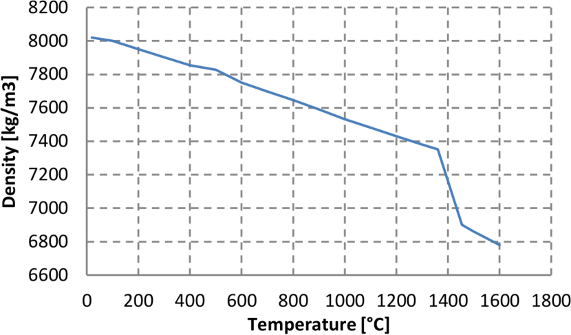
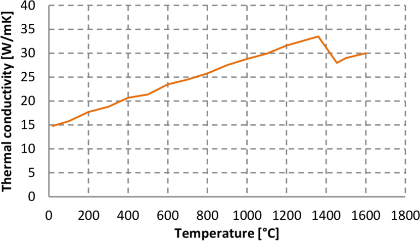
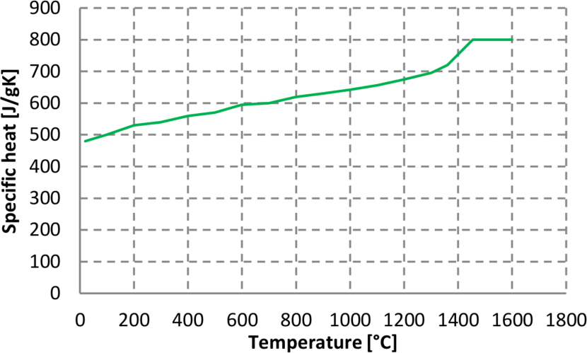
The example is designed to be simple, but suitable enough to compare the accuracy and efficiency of models (2) and (3) with respect to model (1). According to this, the object of simulation is the printing of a 10x10x10 cube on top of a 110x110x20 metal substrate. Different materials are selected for the cubic sample and the build plate: while the former is made of Maraging steel M300, the latter is composed of Stainless Steel (SS) 304L. Bulk temperature-dependent thermal properties of SS 304L [23] are represented in Fig. 5. On the other hand, Tab. 2 prescribes constant density and specific heat values for M300, due to lack of temperature-dependent data, and the M300 powder is assumed to have 54 % of relative density.
| Temperature | Density | Specific heat | Conductivity |
|---|---|---|---|
| 20.0 | 8,100 | 500 | 14.2 |
| 600.0 | 21.0 | ||
| 1,300.0 | 28.6 | ||
| 1,600.0 | 28.6 |
The printing process considers a layer thickness of 30 . Therefore, a total number of 333 layers are deposited to build the sample. The values of the remaining process parameters are detailed in Tab. 3. Note that there is no information regarding the scanning path, because the simulation considers a layer-by-layer deposition sequence. This means that the printing of a complete layer is simulated in a single time step. As a result, the simulation follows an alternating sequence in time consisting of:
-
(1)
Printing step: A new layer is activated, i.e. added into the computational domain, and the problem is solved applying the energy input necessary to fuse the powder of the whole layer. The time increment is given by the scanning time.
-
(2)
Cooling step: The problem is solved without heat application to account for the time lowering the plate, recoat time and laser relocation. Here, the time step is the recoating time.
| Power input | ||
| Scanning time | ||
| Recoating time | ||
| Absorption coefficient | - | |
| Layer thickness | ||
| Plate temperature |
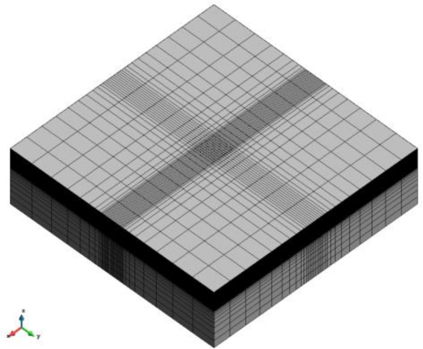
Fig. 6 shows the FE discretizations of the three tested models. All three cases consider structured meshes of varying size to adequately capture the physics of the process. In particular, a finer layer-conforming mesh is prescribed for the fabricated part, whereas a coarser mesh is used away from the printed part. As observed in Tab. 4, the mesh size decreases one order of magnitude from the HF model to the VDA-PP and VDA-P ones.
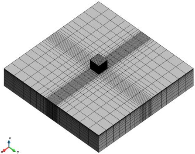
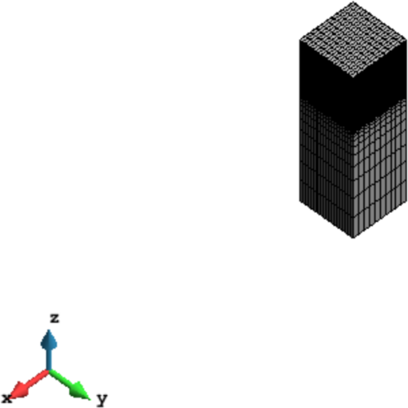
| Model | Mesh size [DoFs] | Runtime []-[%] |
|---|---|---|
| HF | 274.5k | 17.6 - 100 |
| VDA-PP | 66.5k | 1.3 - 7.4 |
| VDA-P | 49.9k | 0.8 - 4.5 |
Concerning the boundary conditions, the top surfaces of the three models are subject to heat transfer through the surrounding air with an HTC of 10 [W/m2C] and air temperature of 20 [C]. On the other hand, the same HTC and environment temperature are assigned at the lateral and bottom walls of the build chamber.
The last ingredient is to characterize the BCs at the solid-powder and part-plate contacting surfaces, by establishing the VDA parameters for the VDA solid-powder (virtual powder) and the VDA part-plate (virtual plate). Recall that only the first applies to the VDA-PP model, whereas both apply to the VDA-P one.
Both VDAs adopt the full Dirichlet variant (cf. (1E-Q1-D) in Tab. 1) described at the end of Sect. 3 with a single linear Lagrangian FE and without geometrical correction factors, for the sake of reducing the number of unknown parameters. In particular, the only ones that need estimation are the virtual domain thicknesses and and the virtual domain environment temperature .
The strategy for such estimation is based on simple calibration with respect to the HF model. Let us explain the procedure step-by-step to model the virtual powder (analogous for the virtual plate). First, the temperature distribution of the HF model is analysed to identify the region concentrating the strongest gradients. As shown in Fig. 7 for the virtual powder, at about 14 away from the part, the temperature drops to 90 [C]. Further away, the thermal gradients are apparently smoother. Therefore, is set to 90 [C] and is initially approximated by 14 . Calibration with respect to the thermal history of the HF model at a selected point follows to correct to the final value. VDA parameter values obtained with this approach are listed in Tab. 5.
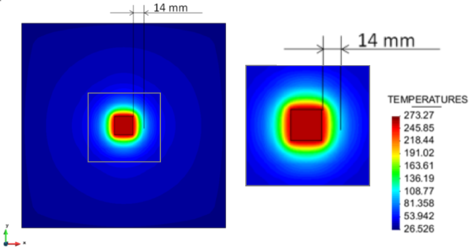
| Domain | VDA thickness | |
|---|---|---|
| Powder | 10 | 90 |
| Plate | 11 | 20 |
The numerical experiments for this example are supported by the in-house research software COupled MEchanical and Thermal (COMET) [5] and GiD [9, 22] as a pre- and postprocessing software. Figs. 8 and 9 compare the temperature evolutions of the reduced models against the reference HF model, at a point located in the middle of the bottom surface of the part. As observed, both VDA-PP and VDA-P are capable of reproducing the thermal response of the HF model with errors bounded by 10 % and 20 % with the Dirichlet VDA variant. The VDA-P is clearly a little less accurate than the former, as expected. However, as seen in Tab. 4, the computational running times of the VDA models are one order of magnitude less than the HF model. This showcases the ability of the new formulation to approximate the response of a high-fidelity model, but with significantly increased efficiency, and it opens the path for larger scale and experimentally-based simulations, such as the one in the next section.
Further experiments were carried out with the VDA-PP model to assess the other VDA discrete forms in Tab. 1. Taking the same parameters as with the Dirichlet case, extra quantities and were not estimated, they were set to 1,000 [W/m2C] and 10 [W/m2C]. Results in Fig. 8(b) show that more accurate discretizations, lead to better approximations of the thermal response, as expected.
4.2. Verification and validation against physical experiments
4.2.1. Experimental campaign
An experimental campaign took place at the Monash Centre for Additive Manufacturing (MCAM) in Melbourne, Australia, with the purpose of (1) calibrating experimentally the thermal analysis FE framework described in Sect. 2 and (2) assess the novel VDA model presented in Sect. 3.
The printing system employed for the experiments is the EOSINT M280 from Electro Optical Systems (EOS) GmbH. It uses an Yb-fibre laser with variable beam width and power up to 400 [W]. The printing process is carried out in a closed 250x250x325 chamber subject to a laminar flow of argon that prevents oxidation.
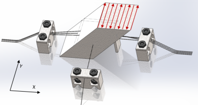
The printed specimen is an oblique square prism with the lower base located in the centre of the building plate and a 45-degrees slope, as shown in Fig. 10. Cross section dimensions are 30x30 and the height is 80 [mm].
Eight thermocouples for temperature measurements are inserted into 0.78 [mm] diameter holes at the upward and downward facing lateral surfaces of the prism (CH1-4 and CH7-8) or in the powder bed (CH5-6). The position of the channels is indicated in Tab. 6 and Fig. 11. The printing job was interrupted at 20.58 [mm] height to install the thermocouples on a set of supporting structures that were printed together with the prism, as shown in Fig. 12.
K-type thermocouples and a Graphtec GL-900 8 high-speed data-logger are used for data gathering. The sampling rate of the data logger is 1 and the time constant of the thermocouples is 7 . As thermocouples are not welded and can move inside the hole, their measurements can be perturbed.
| Channel | (x,y,z) |
|---|---|
| CH1 | (129,125,60) |
| CH2 | (129,125,63) |
| CH3 | (129,120,63) |
| CH4 | (143,125,63) |
| CH5 | (157,125,61.5) |
| CH6 | (157,125,60) |
| CH7 | (156.5,125,63) |
| CH8 | (156.5,120,63) |
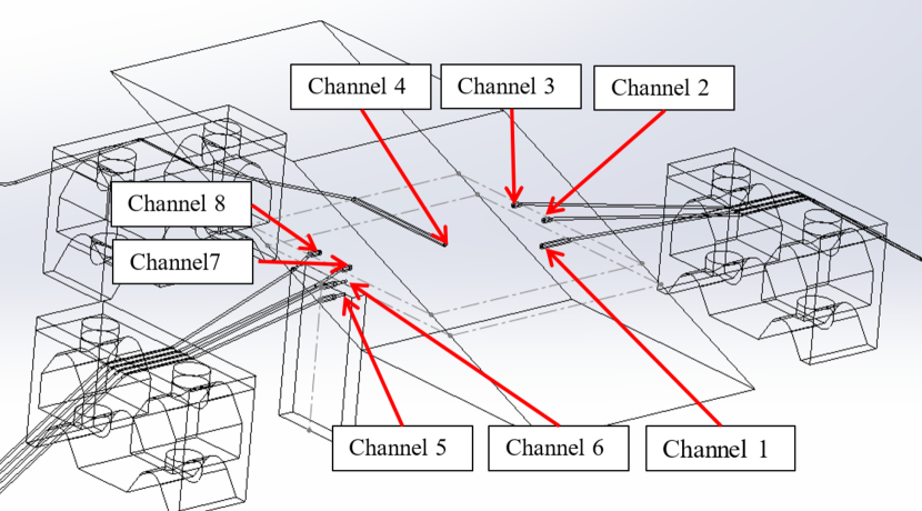
The process parameters used for the printing job are described in Tab. 7. The layer thickness is set to 30 . This means that 647 layers are deposited in about 3.5 [h] to build the samples. As observed, the recoat and laser relocation time varies between odd and even layers.
| Power input | ||
|---|---|---|
| Scanning speed | ||
| Layer thickness | ||
| Hatch distance | ||
| Beam offset | ||
| Recoat time (odd layers) | ||
| Recoat time (even layers) |
Regarding the scanning strategy, the laser travels along the y direction back and forth for each layer, as shown in Fig. 12. Note that the number of hatches drawn does not correspond to the actual number of hatches, which is a much higher value, according to the laser beam size.
The printed samples are made of Ti6Al4V Titanium alloy. The temperature-dependent properties of the bulk material, covering the range from room temperature to fusion temperature, are available in [8]. The base plate is made of CP Ti, a material with similar thermal properties as those of Ti64. Complementary experiments in [8] estimated the relative density of Ti64 powder at around 54 % of the density of the bulk material at room temperature.
Fig. 13 describes the experimental data gathered at the eight thermocouple channels. During the printing of the first layers, the thermocouples are close to the laser and a sharp and highly oscillatory temperature build-up takes place. This trend stabilizes a little before the hundredth layer, when the thermocouples are far enough from the laser spot. Then, the temperature evolution enters a slowly-cooling quasi steady-state regime, until the process finishes and the temperature falls to room temperature.
4.2.2. Methodology
The numerical experiments were supported by a framework consisting of: (1) FEMPAR [2], an advanced object-oriented parallel FE library for large scale computational science and engineering, (2) Dakota [1], a suite of iterative mathematical and statistical methods for parameter estimation, sensitivity analysis and optimization of computational models, and (3) TITANI 8, a High Performance Computer (HPC) cluster at the Universitat Politècnica de Catalunya (Barcelona, Spain).
Such advanced computational framework, integrating FEA tools with scientific software for parameter exploration on a HPC platform, has not been previously observed in the literature related to the numerical simulation of metal AM processes, but it is very convenient to carry out the verification and validation tasks at the scale of the experiment.
| Nodes | 5 DELL PowerEdge R630 |
|---|---|
| CPUs | 2 x Intel Xeon E52650L v3 (1.8GHz) |
| Cores | 12 cores per processor |
| Cache | 30 MB |
| RAM | 256 GB |
| Local disk | 2 x 250 GB SATA |
An overview of the procedure followed during the numerical tests is:
- (1)
-
(2)
Implementation of an interface to communicate Dakota with FEMPAR.
-
(3)
Design and implementation of a physically accurate reference (HF) heat transfer model.
-
(4)
Calibration and validation of the HF model against experimental data generated at the MCAM research centre.
-
(5)
Repeat (3) and (4) for two additional HTC-PP and VDA-PP reduced HPC models in TITANI. Comparison of the reduced-domain variants with the full-domain HF model.
According to this, three different numerical models were tested, the only difference among them being how heat loss through the powder bed is accounted for. In the HF model, the purpose is to maximize the accuracy of the model, by including the powder bed into the computational domain of analysis, to establish a numerical reference for the reduced models.
In the HTC-PP model, the powder-bed is excluded from the computational domain and heat loss through the powder bed is modelled with a constant heat conduction boundary condition at the solid-powder contact surfaces. The VDA-PP model adopts the same hypotheses of the HTC-PP model, except for the computation of the HTC at the solid-powder interfaces, which is derived from Eq. (25), considering a single quadratic element (cf. (1E-Q2) in Tab. 1) to solve the VDA 1D heat conduction problem.
The calibration is done w.r.t. the measurements in thermocouple channels CH2 and CH4, separated 14 mm horizontally. Only measurements during printing are considered; the cooling stage is simulated, but not calibrated. The numerical response is then compared with the experimental data of CH8, one of the furthest from CH2 and CH4, as a way to validate the model. Remaining thermocouples are either close to CH2, CH4, CH8, or outside the sample.
An important feature is that both VDA-PP and HTC-PP models inherit all the simulation data (process parameters, material properties,…) from the HF model and only the relevant parameters of each model are estimated. Tab. 9 gathers all the simulation data from the three models and highlights the calibration parameters of the reduced models.
4.2.3. Calibration of the powder-bed model
The reference model that will be used later to assess the accuracy and performance of the VDA model must reproduce as closely as possible the physical process of metal deposition. Likewise, the size of the simulation must be chosen to enable a full sensitivity analysis and iterative parameter estimation in reasonable computational times.
A locally accurate simulation of the metal deposition process must include the powder-bed in the computational domain, the FE mesh must conform to the printed layers, the mesh size must be smaller than the laser beam spot size, and the scanning path must be tracked element by element.
However, complying with these requirements is not always possible from the computational point of view. For instance, in this experiment, assuming a uniform mesh with element size 50x50x30 , a single layer of the specimen would be composed of 360,000 elements to be printed in 360,000 time steps.
Besides, the focus of this work is on the thermal analysis at the part scale, as commented in Sect. 1. This allows us to control the problem size and the number of time steps, by relaxing the previous discretization requirements with suitable approximations.
The most relevant simplification in this work is the adoption of a layer-by-layer activation strategy, as in Sect. 4.1. Even though this assumption is computationally very appealing, it sacrifices the local thermal history of the response. However, it allows us to recover average thermal responses, as discussed in [8], and enables parametric exploration of the computational model in moderate times. In any case, regardless of the deposition sequence, the reference HF model is, by construction, more accurate than the reduced-domain VDA-PP and HTC-PP versions.
As a result of the previous considerations, the FE discretization is a structured mesh of 9,565,788 hexahedral elements and 9,742,768 nodes. As observed in Fig. 14(a), the FE mesh is a box containing the printed specimen, the building plate, and the powder bed. Supporting structures of the thermocouples are not included in the analysis, because they are far and small enough to have little influence in the results at the specimen.
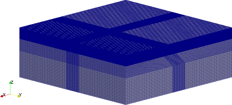

A static mesh is employed throughout the simulation. Element size was determined with a convergence test and it varies, depending on the region of the model. Fine 1x1x0.03 [mm3] elements are prescribed at the simulated region, while larger mesh sizes are specified elsewhere. Note that, as a result of the layer-averaging in time and using a uniform heat source distribution, the mesh size no longer needs to be smaller than the laser spot size.
The numerical simulation begins after placing the thermocouples and resuming the job. It continues with the deposition of the remaining 647 layers and finishes with the cooling of the whole ensemble. This amounts to almost 13,000 [s] of deposition process.
All simulation data is listed in Tab. 9. Some comments arise on the parameter values:
-
(1)
The heat absorption coefficient, estimated at 70 %, is the most sensitive parameter of the model, as also observed in [7].
- (2)
-
(3)
Temperatures of air, powder and plate were measured in the chamber. They suffer variations throughout the process, but the numerical model is barely sensitive to them, with the exception of plate temperature. For this quantity, an estimated evolution law is assumed in Tab. 10, taking into account that the building plate is heated during the printing phase.
-
(4)
The dimensions of the numerical experiment (mesh size and number of time steps) can only be appropriately dealt with parallel computing techniques. Still, the calibration procedure was rather slow. For instance, using 20 CPUs of TITANI, the execution time of a single evaluation of the HF model was approximately 50 [h].
| Parameter | HF model | HTC-PP model | VDA-PP model | Units |
| Process parameters | ||||
| Layer thickness | 30 | m | ||
| Scanning speed | 5.6 | mm/s | ||
| Backward speed (odd layer) | 2.8 | mm/s | ||
| Backward speed (even layer) | 2.1 | mm/s | ||
| Laser power | 280 | W | ||
| Laser efficiency | 70 | % | ||
| Material properties | ||||
| Bulk thermal properties | In [8] | - | ||
| Powder thermal properties | In Tab. 11 | - | In Tab. 11 | - |
| Boundary conditions | ||||
| HTC air | 10 | W/m2C | ||
| Air temperature | 35 | C | ||
| HTC at chamber wall | 10 | W/m2C | ||
| Temperature at chamber wall | 93 | C | ||
| HTC at plate | 10 | W/m2C | ||
| Platform temperature | In Tab. 10 | - | ||
| Equivalent HTC solid-powder | - | 21 | - | W/m2C |
| Powder temperature | 93 | C | ||
| Initial temperature | 93 | C | ||
| Virtual powder model data | ||||
| Thickness | - | - | 36 | mm |
| HTC solid-VDA | - | - | 4,150 | W/m2C |
| HTC VDA-powder | - | - | 1,000 | W/m2C |
| Volume factor | - | - | 1 | - |
| Surface factor | - | - | 1 | - |
| Problem size | ||||
| Mesh size | 9,742,768 | 696,199 | nodes | |
| Number of layers | 647 | layers | ||
| Number of time steps | 1,434 | steps | ||
| Activation strategy | layer-by-layer | - | ||
| Computational cost | ||||
| Number of CPUs | 20 | CPUs | ||
| Execution time | 50 | 3 | h | |
| Time [s] | Temperature [C] |
|---|---|
| 0.0 | 93.0 |
| 11,470.0 | 93.0 |
| 12,000.0 | 35.0 |
| 15,000.0 | 35.0 |
| Temperature [C] | Conductivity [W/mC] |
|---|---|
| 20.0 | 0.288 |
| 200.0 | 0.407 |
| 300.0 | 0.466 |
| 400.0 | 0.520 |
| 500.0 | 0.573 |
| 600.0 | 0.630 |
| 700.0 | 0.684 |
| 800.0 | 0.746 |
| 900.0 | 0.808 |
| 1,100.0 | 0.904 |
| 1,227.0 | 0.976 |
| 1,500.0 | 1.115 |
| 1,600.0 | 1.168 |
| 1,660.0 | 1.252 |
Fig. 16(a) and Tab. 12 compare the numerical response with the experimental measurements. A very good agreement of predicted values and average rates in time can be observed during the whole printing process, both for the reference calibration channels, namely CH2 and CH4, and the validation channel CH8.
| Channel | MAE [C] | MRE [%] |
|---|---|---|
| CH2 | 2.4 | 1.0 |
| CH4 | 6.3 | 2.1 |
| CH8 | 5.0 | 1.5 |
4.2.4. Assessment of the HTC-PP model
Exclusion of the powder-bed from the computational domain leads to a significant reduction in the size of the problem. In this case, the FE mesh (Fig. 14(b)) consists of 647,856 elements and 696,199 nodes. As a result, the HTC-PP model can be solved with significantly less computational resources and time than the previous model, i.e. in 3 [h] using 20 CPUs, and the parametric exploration is also much faster.
The HTC model is characterized by modelling heat transfer through the powder-bed with a constant heat conduction boundary condition on the solid-powder contact surfaces. For calibration against the experimental measurements, all the simulation data is the same as the one of the HF model and the only variable is the HTC of the aforementioned boundary condition.
To interact with Dakota, the parameter estimation problem is formulated as an optimization problem of minimizing the least-squares error between data and variable-dependent response. The optimization problem is solved with a derivative-free local method (pattern search) until convergence.
To start the least-squares solver, the HTC can be initially estimated as
| (28) |
evaluated in the range of observed temperatures (200-400 [C]). Here, is the conductivity of the powder and is the virtual loose powder thickness of the VDA. Using this rule of thumb, the HTC is initially set at 13-17 [W/m2C] and converges to 21 [W/m2C].
Concerning the numerical results, as seen in Fig. 17 and Tab. 13, the simplification of the physics (exclusion of powder-bed + equivalent boundary condition) has obvious negative consequences in the accuracy. Besides, average rate of initial temperature build-up and cooling rate at the quasi-steady state regime are slightly different. In spite of this, the maximum error of the HTC-PP model with respect to the HF one is bounded by 15 %, even for the CH8 channel.
| HF model | experiments | |||
|---|---|---|---|---|
| Channel | MAE [C] | MRE [%] | MAE [C] | MRE [%] |
| CH2 | 6.7 | 2.8 | 4.5 | 1.9 |
| CH4 | 8.3 | 2.8 | 5.5 | 1.8 |
| CH8 | 15.0 | 4.3 | 18.8 | 5.4 |
4.2.5. Assessment of the VDA-PP model
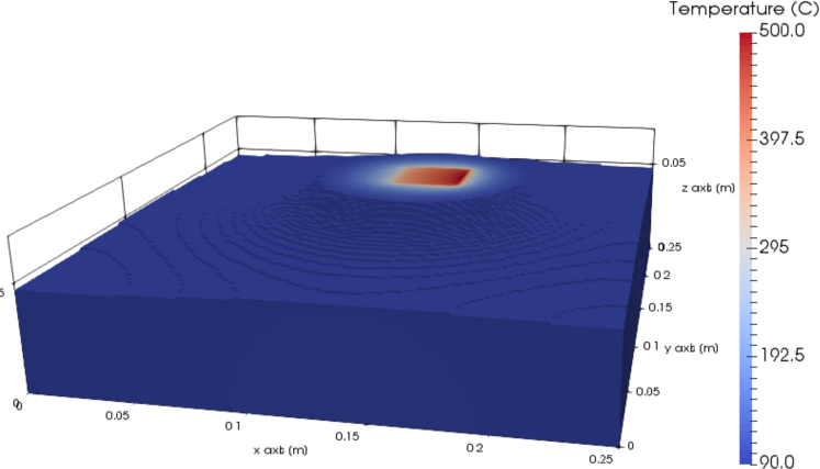
As seen in the contour plot of temperatures in Fig. 18(a), if the nodal values below the initial temperature of the powder are filtered, it is exposed that thermal gradients concentrate around the printed region.
Taking the FE mesh and the simulation data from the HTC-PP model, the Dakota least-squares solver was reformulated for the VDA-PP model. Some parameters of the VDA-PP model can be fixed to reduce the number of calibration variables. For instance, the volume and surface factors and can be set to 1, according to the shell-like shape of the VDA region.
As a result of this, the experimental calibration variables are now the thickness of the VDA and the HTC at the solid-VDA interface . The HTC at the VDA-powder interface is also ruled out, after detecting low sensitivity to this parameter. However, its value should be large enough to have temperatures close to the initial temperature of the powder at the virtual boundary.
As for the initial approximations, from Figure 18(a) the VDA thickness is set to 30 [mm], whereas the HTC solid-VDA is set to 3,000-4,000 [W/m2C], which is in the range of typical values of HTC for metal-sand contact surfaces in sand casting.
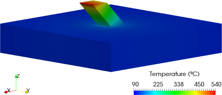
The numerical results in Fig. 19 and Tab. 14 show that the VDA-PP model is successfully able to recover the accuracy of the HF model, at the same reduced computational cost of the HTC-PP model. In particular, average rates of temperature at initial build-up and quasi-steady state regime match pretty well; the only mismatch is observed at the cooling phase, where the VDA-PP model overestimates the thermal inertia of the system.
| HF model | experiments | |||
|---|---|---|---|---|
| Channel | MAE [C] | MRE [%] | MAE [C] | MRE [%] |
| CH2 | 3.6 | 1.5 | 3.6 | 1.5 |
| CH4 | 2.0 | 0.7 | 4.5 | 1.5 |
| CH8 | 2.0 | 0.6 | 6.5 | 1.9 |
5. Conclusions
This work introduces a new rationale for physics-based model reduction in the thermal FE analysis of metal AM by powder-bed fusion methods, the Virtual Domain Approximation (VDA). In view of the locality of the process, it is reasonable to exclude regions of low physical relevance from the domain of analysis to reduce the size of the problem. However, lack of experimental data hinder proper estimation of heat loss through the neglected regions and rather simple approximations have been considered so far. By contrast, the VDA is thought to integrate the physics being neglected to evaluate heat loss through an excluded region. Inspired by existing methods in casting solidification, it consists in replacing the 3D FE model at the low-relevance region (e.g. loose powder bed, building plate) with a 1D heat conduction problem. Following this, the 1D problem is discretized at convenience and reformulated as a temperature-dependent Robin-type boundary condition for the 3D model in the reduced domain.
Using this approach, reduced models obtained by either excluding the powder bed or the powder bed and the building plate were derived and confronted with (1) a reference complete model and (2) the same reduced model, but with a constant boundary condition, i.e. constant HTC and environment temperature. As observed in the numerical experiments, the computational benefit of meshing a smaller geometry (the simulation time is reduced one order of magnitude) is accompanied by increased accuracy with respect to (2). In fact, the new method mostly recovers the thermal response predicted by (1) with the same computational cost of (2). Hence, this domain reduction strategy arises as an alternative that strikes good balance between efficiency and accuracy.
Even using reduced model variants, experimental validation and industrial applications are still challenged by high computational cost and uncertainty of the material and process parameters. To deal with this issue, this work turns to a methodology unprecedented in the field: an HPC platform that brings together (1) FEMPAR-AM, a FE model for the simulation of AM processes, designed to efficiently exploit distributed-memory supercomputers; and (2) Dakota, a suite of iterative mathematical and statistical methods for parametric exploration of computational models. As shown in the MCAM experiment, this advanced framework enables fast and automatized sensitivity analysis and parameter estimation. Hence, this kind of synergy may be useful in metal AM, not only to address verification and validation, but also for practical optimization problems.
One remaining question is to study the method for builds with curved shapes. The VDA assumes unidimensional heat loss, normal to the discrete interface. This is optimal for flat surfaces, but for smooth ones, it may lead to an underestimation of heat loss that, in some cases, can be compensated with simple geometrical correction factors proposed in Sect. 3.
Another interesting line of work is to push ahead the VDA capabilities, by reducing the domain up to the last simulated layers. In this scenario, the domain is thought as moving upwards to track the growth of the geometry, while keeping its size controlled either with a fixed or error-based criterion.
Acknowledgements
Financial support from the EC - International Cooperation in Aeronautics with China (Horizon 2020) under the EMUSIC project (Efficient Manufacturing for Aerospace Components USing Additive Manufacturing, Net Shape HIP and Investment Casting), the EC - Factories of the Future (FoF) Programme under the CAMan Project (Computer Aided Technologies for Additive Manufacturing) within Horizon 2020 Framework Programme and the Spanish Government-MINECO-Proyectos de I+D (Excelencia)-DPI2017-85998-P-ADaMANT-Computational Framework for Additive Manufacturing of Titanium Alloy are gratefully acknowledged. E. Neiva gratefully acknowledges the support received from the Catalan Government through a FI fellowship (2019 FI-B2-00090; 2018 FI-B1-00095; 2017 FI-B-00219). E. Salsi gratefully acknowledges the support received from the European Union’s Horizon 2020 research and innovation programme under the Marie Skłodowska-Curie Grant Agreement No. 746250. S. Badia gratefully acknowledges the support received from the Catalan Government through the ICREA Acadèmia Research Program. Financial support to CIMNE via the CERCA Programme / Generalitat de Catalunya is also acknowledged. The authors thankfully acknowledge the computer resources at TITANI by CaminsTECH, the support provided by O. Colomés, concerning the usage of Dakota, and the help from J. J. Moya in the numerical experiments. The experimental work is funded by the Science & Industry Endowment Fund program RP04-153 Manufacturing a small demonstrator aero-engine entirely through additive manufacturing and Australia Research Council IH130100008 Industrial Transformation Research Hub for Transforming Australia’s Manufacturing Industry through High Value Additive Manufacturing, including financial support from Safran Power Units and Amaero Engineering.
References
- Adams et al. [2016] B. Adams, L. Bauman, W. Bohnhoff, K. Dalbey, M. Ebeida, J. Eddy, M. Eldred, P. Hough, K. Hu, J. Jakeman, J. Stephens, L. Swiler, D. Vigil, and T. Wildey. Dakota, a multilevel parallel object-oriented framework for design optimization, parameter estimation, uncertainty quantification, and sensitivity analysis: Version 6.0 user’s manual. Sandia Technical Report SAND2014-4633, July 2014. Updated November 2016 (Version 6.5), 2016.
- Badia et al. [2018] S. Badia, A. F. Martín, and J. Principe. FEMPAR: An object-oriented parallel finite element framework. Arch. Comput. Methods Eng., 25(2):195–271, 2018.
- Bergman et al. [2011] T. L. Bergman, F. P. Incropera, D. P. DeWitt, and A. S. Lavine. Fundamentals of heat and mass transfer. John Wiley & Sons, 2011.
- Cervera et al. [1999] M. Cervera, C. Agelet De Saracibar, and M. Chiumenti. Thermo-mechanical analysis of industrial solidification processes. International Journal for Numerical Methods in Engineering, 46(9):1575–1591, 1999.
- Cervera et al. [2002] M. Cervera, C. Agelet de Saracibar, and M. Chiumenti. Comet: Coupled mechanical and thermal analysis. data input manual. Barcelona: International Center for Numerical Methods in Engineering (CIMNE), 2002.
- Chiumenti et al. [2008] M. Chiumenti, C. A. de Saracibar, and M. Cervera. On the numerical modeling of the thermomechanical contact for metal casting analysis. Journal of Heat Transfer, 130(6):061301, 2008.
- Chiumenti et al. [2017a] M. Chiumenti, X. Lin, M. Cervera, W. Lei, Y. Zheng, and W. Huang. Numerical simulation and experimental calibration of additive manufacturing by blown powder technology. part i: thermal analysis. Rapid Prototyping Journal, 23(2):448–463, 2017a.
- Chiumenti et al. [2017b] M. Chiumenti, E. Neiva, E. Salsi, M. Cervera, S. Badia, J. Moya, Z. Chen, C. Lee, and C. Davies. Numerical modelling and experimental validation in selective laser melting. Additive Manufacturing, 18(Supplement C):171 – 185, 2017b. ISSN 2214-8604. doi: https://doi.org/10.1016/j.addma.2017.09.002.
- Coll et al. [2016] A. Coll, R. Ribó, M. Pasenau, E. Escolano, J. Perez, A. Melendo, A. Monros, and J. Gárate. GiD v.13 User Manual, 2016.
- Dai and Shaw [2002] K. Dai and L. Shaw. Distortion minimization of laser-processed components through control of laser scanning patterns. Rapid Prototyping Journal, 8(5):270–276, 2002.
- Dantzig and Wiese [1985] J. A. Dantzig and J. W. Wiese. Modeling of heat flow in sand castings: Part II. Applications of the boundary curvature method. Metallurgical Transactions B, 16(2):203–209, 1985. doi: 10.1007/BF02679712.
- Denlinger et al. [2016] E. R. Denlinger, V. Jagdale, G. V. Srinivasan, T. El-Wardany, and P. Michaleris. Thermal modeling of Inconel 718 processed with powder bed fusion and experimental validation using in situ measurements. Additive Manufacturing, 11:7–15, 2016. ISSN 2214-8604.
- Hong et al. [1984] C. Hong, T. Umeda, and Y. Kimura. Numerical models for casting solidification: Part I. The coupling of the boundary element and finite difference methods for solidification problems. Metallurgical Transactions B, 15(1):91–99, 1984. doi: 10.1007/BF02661066.
- Irwin and Michaleris [2016] J. Irwin and P. Michaleris. A Line Heat Input Model for Additive Manufacturing. Journal of Manufacturing Science and Engineering, 138(11):111004–111004–9, 2016.
- Kollmannsberger et al. [2018] S. Kollmannsberger, A. Özcan, M. Carraturo, N. Zander, and E. Rank. A hierarchical computational model for moving thermal loads and phase changes with applications to selective laser melting. Computers and Mathematics with Applications, 75(5):1483 – 1497, 2018.
- Kolossov et al. [2004] S. Kolossov, E. Boillat, R. Glardon, P. Fischer, and M. Locher. 3d FE simulation for temperature evolution in the selective laser sintering process. International Journal of Machine Tools and Manufacture, 44(2–3):117–123, 2004.
- Li et al. [2019] C. Li, M. F. Gouge, E. R. Denlinger, J. E. Irwin, and P. Michaleris. Estimation of part-to-powder heat losses as surface convection in laser powder bed fusion. Additive Manufacturing, 2019.
- Lindgren [2014] L.-E. Lindgren. Computational welding mechanics. Elsevier, 2014.
- Lindgren and Lundbäck [2018] L.-E. Lindgren and A. Lundbäck. Approaches in computational welding mechanics applied to additive manufacturing: Review and outlook. Comptes Rendus Mécanique, 346(11):1033–1042, 2018.
- Lindwall et al. [2018] J. Lindwall, A. Malmelöv, A. Lundbäck, and L.-E. Lindgren. Efficiency and accuracy in thermal simulation of powder bed fusion of bulk metallic glass. JOM, pages 1–6, 2018.
- Lu et al. [2018] X. Lu, X. Lin, M. Chiumenti, M. Cervera, J. Li, L. Ma, L. Wei, Y. Hu, and W. Huang. Finite element analysis and experimental validation of the thermomechanical behavior in laser solid forming of ti-6al-4v. Additive Manufacturing, 21:30–40, 2018.
- Melendo et al. [2016] A. Melendo, A. Coll, M. Pasenau, E. Escolano, and A. Monros. Gid home, 2016. URL www.gidhome.com. [Online; accessed Dec-2018].
- Mills [2002] K. C. Mills. Recommended values of thermophysical properties for selected commercial alloys. Woodhead Publishing, 2002.
- Nastac [1998] L. Nastac. A monte carlo approach for simulation of heat flow in sand and metal mold castings (virtual mold modeling). Metallurgical and Materials Transactions B, 29(2):495–499, 1998.
- Neiva et al. [2019] E. Neiva, S. Badia, A. F. Martín, and M. Chiumenti. A scalable parallel finite element framework for growing geometries. application to metal additive manufacturing. International Journal for Numerical Methods in Engineering, 119(11):1098–1125, 2019.
- Parry et al. [2016] L. Parry, I. Ashcroft, and R. Wildman. Understanding the effect of laser scan strategy on residual stress in selective laser melting through thermo-mechanical simulation. Additive Manufacturing, 12:1–15, 2016.
- Patil et al. [2015] N. Patil, D. Pal, H. Khalid Rafi, K. Zeng, A. Moreland, A. Hicks, D. Beeler, and B. Stucker. A Generalized Feed Forward Dynamic Adaptive Mesh Refinement and Derefinement Finite Element Framework for Metal Laser Sintering—Part I: Formulation and Algorithm Development. Journal of Manufacturing Science and Engineering, 137(4):041001, 2015.
- Prabhakar et al. [2015] P. Prabhakar, W. Sames, R. Dehoff, and S. Babu. Computational modeling of residual stress formation during the electron beam melting process for Inconel 718. Additive Manufacturing, 7:83–91, 2015.
- Renishaw [plc] Renishaw(plc). Data sheets - additive manufacturing, 2018. URL https://www.renishaw.com. [Online; accessed Dec-2018].
- Roberts et al. [2009] I. A. Roberts, C. J. Wang, R. Esterlein, M. Stanford, and D. J. Mynors. A three-dimensional finite element analysis of the temperature field during laser melting of metal powders in additive layer manufacturing. International Journal of Machine Tools and Manufacture, 49(12–13):916–923, 2009.
- Sih and Barlow [2004] S. S. Sih and J. W. Barlow. The prediction of the emissivity and thermal conductivity of powder beds. Particulate Science and Technology, 22(4):427–440, 2004.
- Song et al. [2012] B. Song, S. Dong, H. Liao, and C. Coddet. Process parameter selection for selective laser melting of Ti6al4v based on temperature distribution simulation and experimental sintering. The International Journal of Advanced Manufacturing Technology, 61(9-12):967–974, 2012.
- Wohlers [2017] T. Wohlers. Wohlers report 2017. Wohlers Associates, Inc, 2017.