Measurement of tW the production cross-section at 13 TeV with CMS

Abstract:

The inclusive cross-section for tW production in proton-proton collisions at $\sqrt{s}=13$ TeV is measured with a dataset corresponding to an integrated luminosity of 35.9 fb^-1 collected by the CMS experiment. The measurement is performed in events with one electron and one muon, and exploits kinematic differences between the signal and the dominating $t\bar{t}$ background through the use of multivariate discriminants designed to separate the two processes. The measured cross-section of $\sigma=63.1\pm 1.8~{}({\rm stat})\pm 6.0~{}({\rm syst})\pm 2.1~{}({\rm lumi})$ pb is in agreement with standard model expectations.

1 Introduction

Single top quarks are produced via the electroweak interaction. There are three main production channels that can occur in proton-proton (pp) collisions: the exchange of a virtual W boson ($t$ channel), the production and decay of a virtual W boson ($s$ channel) and the associated production of a top quark and a W boson (tW channel).

The tW process was first observed by the CMS [1] and ATLAS [2] Collaborations in 8 TeV pp collisions. This process provides a unique opportunity to study the standard model and its extensions, due to the quantum interference of this process with top quark pair production (${\mathrm{t}\overline{\mathrm{t}}}$). It can also be a probe of the $V_{tb}$ element of the CKM matrix.

The increase in cross-section of the process at 13 TeV and the larger amount of luminosity delivered by the LHC to the CMS detector [3] allows the measurement of the tW production-cross section with a larger precision than ever. This note reports that measurement, fully described in [4].

2 Event selection and signal extraction

In the standard model (SM), a top quark decays almost exclusively into a W boson and a bottom quark. Therefore, the measurement is performed in events with two opposite-sign, different-flavor leptons, targeting the leptonic decays of the two W bosons. Such events are collected using a set of di-lepton and single-lepton triggers. The leading lepton is required to have $p_{T}>$ 25 GeV, while the subleading is required to have $p_{T}>$ 20 GeV.

Figure 1: Distribution of $(n_{\text{jet}},n_{\text{b jet}})$ in events passing the di-leptonic selection [4].

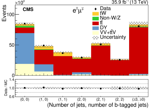
The analysis exploits the different $(n_{\text{jet}},n_{\text{b jet}})$ spectrum between the signal and the different backgrounds present in the dileptonic baseline selection. The distribution is shown in Fig. 1, that shows that indeed the Drell-Yan events contain less jets or b jets, while ${\mathrm{t}\overline{\mathrm{t}}}$ and tW events contain at least one b-tagged jet. Three analysis regions are defined according to they different signal and background composition: a signal-enriched region with events with exactly one jet that is b-tagged (1j1b), and two background-dominated regions with two jets, one with one b-tagged jet (2j1b) and one with two b-tagged jets (2j2b).

Even the more signal-enriched region is still dominated by ${\mathrm{t}\overline{\mathrm{t}}}$ events. Therefore, given there is no single observable that discriminates between tW and ${\mathrm{t}\overline{\mathrm{t}}}$ events, the analysis makes use of multivariate techniques in order to achieve some discrimination.

Figure 2: Comparison of the BDT output in the 1j1b (upper left) and 2j1b (upper right) regions and the $p_{T}$ of the subleading jet in the 2j2b region (lower) distributions after the fit is performed for the observed data and simulated events [4].

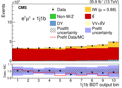
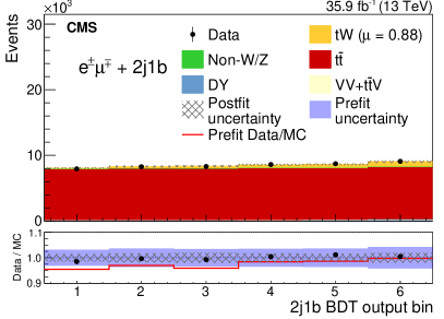
Dedicated boosted decision trees (BDTs) are trained in the 1j1b and 2j1b regions, exploiting the different kinematic and topological differences between ${\mathrm{t}\overline{\mathrm{t}}}$ and tW production. The BDT trained in the 1j1t region profits from the fact that in ${\mathrm{t}\overline{\mathrm{t}}}$ events in this region one of the jets lies outside the acceptance. Therefore important variables used in the training of this BDT are the number of jets with $p_{T}>20$ GeV or the overall transverse boost of the system formed by the two leptons, the jet and the missing transverse momentum. The BDT used in the 2j2b region exploits angular correlations between the leptons, the jet and the missing transverse momentum.

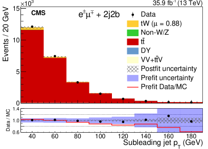
The signal extraction is done by performing a maximum likelihood fit to the distribution of the two BDTs in the 1j1b and 2j2b regions. Additionally, the distribution of the subleading jet $p_{T}$ in events in the 2j2b region is also included in the fit, which is performed simultaneously in the three regions. The distributions employed in the fit are shown in Fig. 2.

The statistical analysis employs a likelihood function, $\mathcal{L}(\mu,\vec{\theta})$, which is a function of the signal strength, $\mu$, and a set of nuisance parameters that model the effect of the systematic uncertainties present in the analysis. The likelihood function is built as the product of Poisson distributions that represent the event counting in each one of the bins of the fitted distributions. Additional log-normal terms are added modeling the priors of each nuisance parameter.

The best estimation of $\mu$ is obtained by minimizing $\mathcal{L}(\mu,\vec{\theta})$ with respect to all of its parameters. The 68% confidence interval is obtained by considering variations of the test statistic used in [5] by one unit from its minimum.

The impact of the statistical uncertainty is determined from the uncertainty of a fit performed fixing all the nuisance parameters to the postfit value of the nominal fit. The impact of the systematic uncertainty is assessed by performing a likelihood fit fixing all the nuisance parameters to the postfit value of the nominal fit, except the one under study.

The systematic uncertainties taken into account are listed in Tab. 1 and account for both experimental uncertainties, as well as theoretical assumptions that are made on the distributions of the signal process and the normalization and distribution of the background processes.

3 Results

The estimated tW signal-strength parameter is $0.88\pm 0.02\text{ (stat.) }\pm 0.09\text{ (syst.) }\pm 0.03\text{ (lumi.) }$, corresponding to a measured cross-section of $63.1\pm 1.8\text{ (stat.) }\pm 6.4\text{ (syst.) }\pm 2.1\text{ (lumi.) }$ pb, consistent with the SM expectations with an uncertainty of 11%. The impact of each source of systematic uncertainty in the fit is shown in Table 1. The uncertainties in the luminosity, trigger and lepton efficiencies have a sizable impact in the estimation of the background yield, which is dominant in all bins of the fit. Therefore these uncertainties have a significant contribution in the final measurement.

Table 1: Estimation of the effect on the signal strength of each source of uncertainty in the fit. Exp erimental and modeling uncertainties affect both the rate and the shape of the templates while background normalizat ion uncertainties affect only the rate [4].

Source	Uncertainty (%)
Experimental
Trigger efficiencies	2.7
Electron efficiencies	3.2
Muon efficiencies	3.1
JES	3.2
Jet energy resolution	1.8
b tagging efficiency	1.4
Mistag rate	0.2
Pileup	3.3
Modeling
${\mathrm{t}\overline{\mathrm{t}}}$ $\mu_{\mathrm{R}}$ and $\mu_{\mathrm{F}}$ scales	2.5
tW $\mu_{\mathrm{R}}$ and $\mu_{\mathrm{F}}$ scales	0.9
Underlying event	0.4
Matrix element/PS matching	1.8
Initial-state radiation	0.8
Color reconnection	2.0
B fragmentation	1.9
Semileptonic B decay	1.5
PDFs	1.5
DR-DS	1.3
Background normalization
${\mathrm{t}\overline{\mathrm{t}}}$	2.8
VV	0.4
Drell–Yan	1.1
Non-W/Z leptons	1.6
${\mathrm{t}\overline{\mathrm{t}}}$V	0.1
MC finite sample size	1.6
Full phase space extrapolation	2.9
Total systematic	10.1
Integrated luminosity	3.3
Statistical	2.8
Total	11.1

References

- [1] CMS Collaboration, “Observation of the associated production of a single top quark and a boson in pp collisions at 8 TeV.” Phys. Rev. Lett. 112 (2014) 231802
- [2] ATLAS Collaboration, “Measurement of the production cross-section of a single top quark in association with a boson at 8 TeV with the ATLAS experiment”, JHEP 01 (2016) 064
- [3] CMS Collaboration, JINST 3 S08004 (2008)
- [4] CMS Collaboration, “Measurement of the production cross section for single top quarks in association with W bosons in proton-proton collisions at TeV”, JHEP 10 (2018) 117
- [5] CMS Collaboration, “Precise determination of the mass of the Higgs boson and tests of compatibility of its couplings with the standard model predictions using proton collisions at 7 and 8 TeV”, Eur. Phys. J. C 75 (2015) 212