Dark, Cold, and Noisy: Constraining Secluded Hidden Sectors
with
Gravitational Waves
Abstract
We explore gravitational wave signals arising from first-order phase transitions occurring in a secluded hidden sector, allowing for the possibility that the hidden sector may have a different temperature than the Standard Model sector. We present the sensitivity to such scenarios for both current and future gravitational wave detectors in a model-independent fashion. Since secluded hidden sectors are of particular interest for dark matter models at the MeV scale or below, we pay special attention to the reach of pulsar timing arrays. Cosmological constraints on light degrees of freedom restrict the number of sub-MeV particles in a hidden sector, as well as the hidden sector temperature. Nevertheless, we find that observable first-order phase transitions can occur. To illustrate our results, we consider two minimal benchmark models: a model with two gauge singlet scalars and a model with a spontaneously broken gauge symmetry in the hidden sector.
I Introduction
With the advent of gravitational wave (GW) astronomy, we can for the first time hope to sense physics that happened before the era of Big Bang Nucleosynthesis (BBN). In fact, gravitational wave observatories on the ground and in space, as well as pulsar timing arrays (PTAs), will be sensitive to the reverberations of spacetime caused by violent first-order phase transitions (PTs) in the very early Universe. Though produced almost 14 billion years ago, these perturbations can still be detectable today, as a contribution to the stochastic gravitational wave background Witten:1984rs ; Hogan:1984hx ; Hogan:1986qda ; Turner:1990rc . (For recent work on this topic, see Refs. Caprini:2015zlo ; Caprini:2018mtu ; Mazumdar:2018dfl and references therein.) The gravitational wave amplitude and frequency spectrum allow us to infer both the properties of the phase transition that generated them and the history of the Universe since then.
It is this connection between stochastic gravitational waves and the particle physics responsible for their emission that we focus on in this paper. In particular, we study scenarios in which gravitational waves are emitted when a scalar field transitions from a local minimum of its potential into the global minimum. We are especially interested in the case that the scalar is part of a “hidden sector”, i.e. a group of particles that interact only very weakly with Standard Model (SM) particles and are therefore extremely challenging to detect directly. In the extreme case where the hidden sector is coupled only via gravity, gravitational waves may provide the only way of studying such new physics scenarios.
In this paper, we expand on past studies of gravitational waves from hidden sector phase transitions Schwaller:2015tja ; Jaeckel:2016jlh ; Addazi:2016fbj ; Baldes:2017rcu ; Addazi:2017gpt ; Tsumura:2017knk ; Aoki:2017aws ; Geller:2018mwu ; Croon:2018erz ; Baldes:2018emh in several ways:
-
(i)
Light hidden sectors. We pay special attention to the possibility that the hidden sector may contain interesting dynamics at sub-MeV temperatures. New particles in the mass range are motivated for instance by the lack of direct detection signals of dark matter. Moreover, gravitational wave signals from low-temperature phase transitions may be easier to detect because the ratio of the gravitational wave energy to the total energy density of the Universe (given by the parameter that will be defined and discussed in Section II.2) can be larger. We will study the interplay between cosmological constraints on sub-MeV particles (in particular the upper limit on the total relativistic energy density, as measured by the parameter ) on the one hand, and the observability conditions for stochastic gravitational waves on the other hand. This will, in particular, require us to investigate in detail the sensitivity of PTAs, which are sensitive to gravitational waves in the relevant frequency range – Hz. A hidden sector phase transition will only be observable if a sufficiently large amount of energy is converted into gravitational waves. This sets a lower limit on the hidden sector energy density. We will present our results as limits on the number of hidden sector degrees of freedom and on the hidden sector temperature.
-
(ii)
Unequal photon and hidden sector temperatures. In the past, it has usually been assumed that the temperatures of the hidden and visible sectors are the same. This, of course, need not be the case: because of their weak coupling, the two sectors may never come into thermal contact. And even if they are heated to the same temperature after inflation, their subsequent evolution may be different. In particular, whenever a heavy particle species becomes non-relativistic and annihilates or decays into lighter species, the corresponding entropy dump into the lighter species delays Hubble cooling. If the numbers of heavy particles are very different in the two sectors, this alone can already lead to substantial temperature differences. For phase transitions at low (sub-MeV) temperatures detectable in PTAs, a temperature difference of the hidden sector with respect to the SM sector is even required, otherwise the additional light degrees of freedom would be inconsistent with cosmology. We will therefore investigate how such temperature differences can affect gravitational wave signals, their detectability, and their interpretation.
-
(iii)
Toy models. We construct two explicit toy models that feature a hidden sector phase transition at sub-MeV scales. We demonstrate that observable gravitational wave signals are possible for narrow strips of parameter space even in light of stringent constraints on additional light degrees of freedom. The first model involves a hidden sector consisting of two scalar fields, the second one is a Higgsed dark photon model. Due to the aforementioned restrictions on the number of light degrees of freedom in the hidden sector, these toy models should cover a large fraction of the model space at sub-MeV energies. We expect that almost any perturbative hidden sector that has been in thermal contact with the SM sector not too far above the electroweak scale and that features an observable first-order phase transition at sub-MeV temperatures should reduce to one of our toy models, or simple variants thereof.
We begin in Section II with a careful discussion of stochastic gravitational wave spectra from phase transitions in the early Universe. We then translate these spectra into sensitivity curves for current and future gravitational wave detectors. This model-independent discussion is complemented in Section III by the introduction of our two toy models, and by the discussion of future gravitational wave constraints on these models. Our conclusions will be summarized in Section IV.
II Gravitational Wave Sensitivity
II.1 Hidden Sector Cosmology
We begin our discussion by reviewing important constraints on hidden sectors, paying special attention to the possibility that the hidden and visible sectors have different temperatures. We define the temperature ratio
| (1) |
where and are the hidden sector and visible sector (photon) temperatures, respectively. A temperature ratio could have been generated already during reheating after inflation, for instance if inflatons decay preferentially into one of the two sectors, and the two sectors never come into thermal contact. Another possible source of temperature differences is early decoupling of two sectors that initially share the same temperature. Whenever a thermalized particle species becomes non-relativistic in one sector, the entropy associated with it is transferred to the remaining particle species, thereby heating that sector up. If one sector contains significantly more heavy particles than the other, values of very different from unity can be expected. In what follows, we will be interested in the case , as we will see that some cosmological constraints are relaxed if the hidden sector is colder than the photons.
This is in particular true for hidden sectors containing particles at the MeV scale or below. (Heavier hidden sectors are essentially unconstrained.) As we will see, sub-MeV hidden sectors are of particular interest for detection in PTAs. The main constraints on hidden particles with masses arise from measurements of the relative abundance of light elements from Big Bang Nucleosynthesis (BBN) Aver:2015iza ; Peimbert:2016bdg , as well as measurements of the Cosmic Microwave Background (CMB) power spectrum Ade:2015xua ; Aghanim:2018eyx . A conflict with these measurements could arise for two reasons: First, the annihilation of a hidden sector species during BBN or recombination might heat up the photon or the neutrino bath, affecting the predicted light element abundances in a detectable way. Second, light hidden sector particles (“dark radiation”) can directly affect the expansion rate of the Universe because the latter is proportional to the total energy density, which in turn is dominated by contributions from relativistic particles until just before recombination. These contributions are parameterized by the effective number of neutrino species, defined as
| (2) |
where and are the energy densities of all relativistic species and of the photons, respectively. In the SM, Mangano:2005cc . The most conservative 95% confidence level (CL) constraint on from 2018 Planck data is at recombination, while an analysis taking into account data on CMB polarization and baryon acoustic oscillations (BAO) yields Aghanim:2018eyx
| (Planck TT, TE, EE + lowE + lensing + BAO) | (3) |
In view of the current tension between the high and low redshift measurements of the Hubble parameter (see 0004-637X-855-2-136 and references therein), this bound may be considered somewhat too strong. Taking all measurements of at face value, the bound is relaxed to
| (Planck TT, TE, EE + lowE + lensing + BAO + ) | (4) |
Formation of light nuclei during BBN imposes the complementary 95% CL constraint Aghanim:2018eyx
| (5) |
assuming remains constant during BBN Shvartsman:1969mm ; Steigman:1977kc ; Scherrer:1987rr ; Patrignani:2016xqp (see for instance Ref. Hufnagel:2017dgo for the impact of relaxing this assumption).
It is convenient to express in Eq. 2 in terms of hidden sector parameters, in particular the temperature and the number of effective relativistic hidden sector degrees of freedom (DOFs) . “Effective” here means that each bosonic degree of freedom contributes one unit to , while each fermionic degree of freedom contributes . This way, can be used directly in the computation of the relativistic energy density. We can distinguish the following cases:
-
1.
Hidden sector in thermal contact with the SM. A hidden sector that is in thermal contact with the photons throughout the BBN (and -annihilation) epoch is disfavored by both the BBN and CMB constraints on : Eq. 4 shows that even a single real scalar degree of freedom () would be inconsistent with the constraint at 95% CL. We will therefore not consider this scenario in the following.
The BBN constraint on is somewhat weaker for a hidden sector which is in thermal contact with the photons only via the neutrinos at the temperature of neutrino decoupling Baumann:2018muz , i.e. which couples efficiently to neutrinos, but not directly to photons. In this case, we find
(6) before the hidden sector particles become non-relativistic and annihilate or decay away into neutrinos, and
(7) afterwards Boehm:2012gr . In these expressions is the effective number of SM neutrino degrees of freedom, and is the number of SM neutrino generations. Here is understood to mean the number of relativistic degrees of freedom in the hidden sector at . The CMB constraint on given in Eq. 4 translates to the bound () at CL if the hidden sector becomes non-relativistic after (before) recombination. In other words, no new light degree of freedom can remain in thermal equilibrium with the SM neutrinos after , even if we use the least stringent of the three cosmology constraints under consideration.
-
2.
Completely decoupled hidden sector. If the hidden sector starts out at early times with a temperature different from the SM bath and never (re-)enters thermal equilibrium with the visible sector, the additional contribution to is
(8) where is now understood to be the effective number of relativistic hidden sector degrees of freedom at hidden sector temperature . The same expression holds if the hidden sector was in equilibrium with the SM sector at early times, but later decoupled while still relativistic.
In the left-hand panel of Fig. 1 we show the CMB and BBN constraints on the hidden sector parameters and based on Eq. 8. The orange and blue regions are excluded at by the BBN and CMB constraints, respectively, while the CMB only bound is shown as a dashed-blue line. Wee see that hidden sectors with more degrees of freedom need to be colder to keep the total hidden sector energy density (and thus ) consistent with the constraints. Even a hidden sector with only one additional degree of freedom () is excluded unless the hidden sector temperature is smaller than times the SM temperature.
Note that for a completely decoupled hidden sector, an important additional constraint may arise from the total matter density of the Universe. As hidden sector particles become non-relativistic, care must be taken that their energy density gets converted into a form of dark radiation in order not to overclose the Universe.
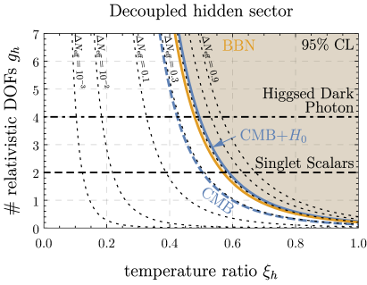
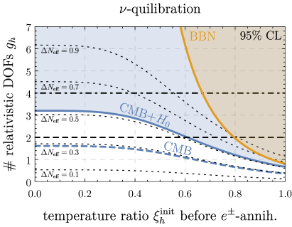
Figure 1: Black dotted contours: the change in as a function of the effective number of relativistic degrees of freedom in the hidden sector () and of the ratio between the hidden and visible sector temperatures (). The left-hand panel is for the case of a hidden sector that is never in thermal equilibrium with SM particles (or has decoupled long before BBN). The right-hand panel is for the “-quilibration” scenario, where the hidden sector (re-)couples with the neutrinos, after the latter have decoupled from the photons. The horizontal axis in the right-hand panel gives , the hidden sector-to-photon temperature ratio before both (re-)coupling and -annihilation. The orange shaded region indicates the BBN constraint on from Eq. 5, while the blue shaded region and blue dashed contour show the CMB constraints with and without the low-redshift measurements of , see Eqs. 3 and 4. The horizontal dashed and dot-dashed lines indicate the number of degrees of freedom in the two toy models discussed in Section III. These figures serve as an update to Refs. Berlin:2017ftj ; Berlin:2018ztp based on the new Planck results Aghanim:2018eyx . -
3.
Hidden sector equilibrates with neutrinos (-quilibration). While the hidden sector cannot be in thermal contact with the photon bath at temperatures around or below the BBN temperature , there is the possibility that it (re-)couples with neutrinos after the latter have lost thermal contact with the photons Berlin:2017ftj ; Berlin:2018ztp . This scenario, which we will dub “-quilibration”, corresponds to the following sequence of events:
![[Uncaptioned image]](/html/1811.11175/assets/x3.png)
where is the photon temperature at neutrino decoupling, is the (photon) temperature at which the hidden sector comes into thermal contact with neutrinos, and is the (photon) temperature at which the hidden sector becomes non-relativistic and its entropy gets dumped back into the neutrino bath. If the hidden sector was ever in thermal contact with the SM at very early times (long before BBN), we denote the temperature at which it lost thermal contact by . Assuming that all hidden sector particles are relativistic when the hidden sector comes into thermal equilibrium with the neutrinos, and that equilibration is quasi-instantaneous, the temperature change experienced by the equilibrating sectors is determined by conservation of energy density. If the temperature ratio between the hidden sector and the photons is prior to BBN, -annihilation, and hidden sector–neutrino (re-)coupling, the temperature ratio after (re-)coupling is
(11) where is the temperature ratio between the neutrino and photon sectors in the Standard Model. Its value is approximately, but not exactly, . A small correction factor arises because of the effect of -annihilation on the neutrino temperature. Equation 11 is valid assuming that -annihilation finishes before the hidden sector equilibrates. The effective number of neutrino species is modified to (14) This shows that returns to in the limit .
When the neutrino/hidden sector temperature drops further below , there are two possibilities for the decoupling of the hidden sector from the neutrinos. The first possibility is that interactions between the neutrinos and the hidden sector particles become too small to maintain equilibrium, resulting in decoupling while the hidden sector is still relativistic. As the hidden sector subsequently becomes non-relativistic, entropy cannot be transferred to the neutrino bath, so the neutrino-to-photon temperature ratio stays at the value given by Eq. 11. at recombination, however, will have decreased compared to Eq. 14 by a factor , possibly violating CMB constraints. Even more problematic, the frozen out non-relativistic hidden sector particles will contribute to the dark matter density, most likely overclosing the Universe. Therefore, we will not consider this case any further.
The second possibility is that the neutrino/hidden sector temperature drops below the masses of the hidden sector particles while the two sectors are still in equilibrium. The hidden sector particles will then annihilate back to neutrinos, thereby reheating the neutrino bath with respect to the photons. Beginning with Eqs. 11 and 14 and using conservation of co-moving entropy yields
(17) for the neutrino-to-photon temperature ratio, and (20) for the effective number of neutrino species after hidden sector decoupling. Unless hidden sector particles have masses , this is the value that will be measured in the CMB.
In the right-hand panel of Fig. 1 we show the excluded regions in the – plane for the -quilibration scenario. We remind the reader that , plotted on the horizontal axis, is the hidden sector-to-photon temperature ratio before both BBN and -annihilation. As before, the orange and blue regions are excluded at 95% CL by BBN and CMB constraints, respectively, while the CMB-only constraint is given by the dashed blue line. BBN constraints are based on Eq. 14, which corresponds to the assumption that hidden sector particles become non-relativistic only after BBN, or, more precisely, after the initial formation of the light elements (4He and D) at MeV Cyburt:2015mya . The CMB constraint is derived from Eq. 20.
II.2 Temperature Dependence of the Gravitational Wave Parameters
We have concluded from Fig. 1 that hidden sectors with a large particle content at masses may be cosmologically allowed, but only if their temperature is substantially lower than the photon temperature (), and their coupling to photons is tiny. The second of these requirements makes it extremely hard to probe such hidden sectors using conventional cosmological, astrophysical, or laboratory methods. This is why we focus here on gravitational waves: if the hidden sector undergoes a strongly first-order phase transition at some point in cosmological history, the gravitational waves emitted in the process may be detectable today as part of the stochastic gravitational wave background. The frequency dependence of the gravitational wave spectrum furthermore contains information about the properties of the phase transition and the subsequent expansion history of the Universe.
The spectra of gravitational waves sourced by cosmological first-order phase transitions depend mainly on three parameters: the strength of the phase transition, , its inverse time scale, , and the temperature at which the transition occurs (nucleation temperature) Turner:1992tz ; Kamionkowski:1993fg ; Grojean:2006bp ; Caprini:2015zlo . In the following, we will define these parameters in terms of particle physics quantities. For phase transitions occurring in a hidden sector, we will in particular discuss their dependence on the temperature ratio .
A first-order phase transition proceeds by the nucleation of bubbles of the new (true vacuum) phase in the background plasma that is still in the old (false vacuum) phase. Thus, the transition begins when the rate at which such bubbles form within a Hubble volume exceeds the Hubble time. The temperature at which this happens is the bubble nucleation temperature . The bubble nucleation rate per unit volume is given by Coleman:1977py ; Callan:1977pt ; Linde:1981zj where is the temperature dependent Euclidean action corresponding to the transition from the false vacuum to the true one. For bubble nucleation at non-zero temperature the time component of the 4-dimensional Euclidean action becomes , i.e. where is the remaining 3-dimensional Euclidean action Linde:1981zj . Assuming and that the phase transition occurs during a radiation dominated epoch such that ( is the radiation energy density and is Newton’s constant), the nucleation criterion evaluates to
| (21) |
Note that here we still assume that all sectors are in thermal equilibrium, and is the total number of relativistic degrees of freedom.111In our analysis, we will use Eq. 21 even for evaluating the nucleation criterion in scenarios with . The resulting is then rescaled to account for the true value of . By doing so, we neglect logarithmic corrections to Eq. 21 arising from the difference between and .
The available energy budget for gravitational wave emission is given by the latent heat , i.e. the absolute change in the energy density, see Ref. Espinosa:2010hh for additional details. The latent heat release normalized to the total radiation density of the Universe, , at the time of the phase transition gives the strength of the phase transition, 222Strictly speaking, we should here distinguish between the temperature at which gravitational waves are emitted (usually referred to as ) and . The two temperatures may be different if the latent heat released during the phase transitions heats the plasma considerably compared to its initial temperature, as could be the case for instance for a phase transition happening during a vacuum-dominated epoch Brdar:2018num ; Ellis:2018mja ; Prokopec:2018tnq ; vonHarling:2017yew ; Bruggisser:2018mrt ; Konstandin:2011dr ; Kobakhidze:2017mru ; Iso:2017uuu ; Bai:2018vik ; Megias:2018sxv ; Hambye:2018qjv ; Caprini:2015zlo ; Randall:2006py . However, in the following we will only consider phase transitions occurring during radiation domination, and we will therefore set in the rest of this paper.
| (22) |
Here, is the change in the potential between the false and the true vacua. Once again, is understood to mean the temperature at the time of the phase transition of the sector in which the phase transition occurs. For a phase transition occurring in the SM (hidden sector), should thus be replaced by the photon (hidden sector) temperature () at the time of bubble nucleation.
It is intuitively clear that larger implies larger gravitational wave amplitudes. If all particle species abundant in the Universe share the same temperature, is simply given by , where is the total number of effective relativistic degrees of freedom. We will instead be interested in a phase transition occurring in a hidden sector whose temperature is different from the photon temperature, in which case the appropriate expression is instead
| (23) | ||||
where and are the numbers of relativistic degrees of freedom in the SM sector and the hidden sector, respectively. As we have seen in Section II.1, CMB and BBN constraints on can only be satisfied if . Then, for fixed , scales approximately proportional to , and consequently
| (24) |
In other words, a large temperature ratio between the visible and hidden sectors at the time of the phase transition reduces the strength of the gravitational wave signal compared to the case where both sectors have similar temperatures.
Gravitational wave signals from phase transitions also depend on the inverse time scale of the phase transition, : a fast transition means that many bubbles form simultaneously, so they are still small when they collide. This results in gravitational wave signals that are weaker and peak at higher frequencies than those from a slow transition. The inverse time scale is given by
| (25) |
where the right-hand side is to be evaluated at the time of bubble nucleation . It is conventional to normalize to the Hubble rate at the time of bubble nucleation, which leads to
| (26) |
Note that, unlike itself, is independent of the temperature ratio .
Besides , , and , gravitational wave spectra in principle depend also on the bubble wall velocity, , i.e. the speed at which bubbles of the true phase expand. We assume an optimistic value , which is well justified for strong phase transitions Bodeker:2017cim . Note that the amplitude of the gravitational wave power spectrum depends linearly on (see Section II.3 for the full dependence), therefore small deviations from will not significantly affect our results.
The key result of the above discussion is that a strong gravitational wave signal and safety from constraints impose opposite conditions on hidden sector models: for compatibility with constraints, is needed, while the scaling of with implies that strong gravitational wave emission from a hidden sector phase transition is only possible if is not too small. In Section III below, we will see explicitly the impact of these conflicting conditions on the parameter space of two toy models. In particular, we will see that for a hidden sector that is completely decoupled from the SM, observable gravitational wave signals are possible for only thin strips of parameter space. For a hidden sector that (re-)enters thermal equilibrium with the neutrinos after the latter have decoupled, Eq. 11 shows that the value of at the phase transition (after hidden sector (re-)coupling) can be significantly larger than the initial temperature ratio . In other words, even though the initial may be small enough to avoid the BBN constraint on , the relevant during the phase transition may be large enough to yield a strong gravitational wave signal. Of course, one still needs to worry about the late-time neutrino-to-photon temperature ratio given by Eq. 17 possibly violating the CMB constraint on .
II.3 Gravitational Wave Spectrum from a Hidden Sector Phase Transition
In what follows we review the possible mechanisms that source gravitational waves during a first-order phase transition. We closely follow Ref. Caprini:2015zlo , but we extend the results from that paper for the case of a hidden sector temperature differing from the photon temperature. The production of gravitational waves in a first-order phase transition can be separated into three stages:
-
1.
Collisions of the bubble walls. Huber:2008hg This contribution depends only on the dynamics of the scalar field (not on the background plasma) and is therefore often referred to as the scalar field contribution. It is usually treated in the “envelope approximation”, which assumes sizable interactions only at the intersection points of the bubble walls and a quick dispersion after the bubble collisions.
-
2.
Collision of sound waves in the plasma generated during bubble expansion Hindmarsh:2015qta . Compared to the contribution arising from bubble wall collisions, this effect lasts longer and is therefore enhanced by a factor of .333Note that it currently remains unclear whether the simulation of this contribution can be extrapolated to very strong transitions with Hindmarsh:2015qta ; Caprini:2015zlo . In addition, for phase transitions with (corresponding to a large number of smaller bubbles being nucleated), the timescale of the transition from sound waves to turbulence is expected to be significantly shorter than a Hubble time. Subsequently, the period of time where sound waves can source gravitational waves is cut short. However, current simulations are unable to make precise predictions about the transition to turbulence in the regime . Therefore the exact efficiency of converting sound waves to turbulence remains unknown Hindmarsh:2017gnf ; Ellis:2018mja .
-
3.
Turbulence in the plasma after the collision of sounds waves, which can last for several Hubble times Caprini:2009yp . This contribution is suppressed by a factor of compared to the sound wave contribution, i.e. only a small part of the sound wave energy budget is converted into turbulent motion Hindmarsh:2015qta . We will optimistically assume .
While a complete description of these contributions requires numerical simulations, it is for our purposes useful to work with an analytic parameterization for the gravitational wave frequency spectra. A suitable functional form for the gravitational wave power spectrum at emission is Huber:2008hg ; Hindmarsh:2015qta ; Caprini:2009yp
| (27) |
where is the critical energy density, with the Hubble rate in the radiation-dominated era is given by . depends on the normalization factor , the velocity factor , the efficiency factors , the exponents and , and the spectral shape function . These parameters are determined for the three contributions separately by fitting to the results of numerical simulations. A summary of the resulting parameter values is given in Table 1.
| Scalar field | Sound waves | Turbulence | |
|---|---|---|---|
| Reference | Huber:2008hg | Hindmarsh:2015qta | Caprini:2009yp |
After its emission, the stochastic gravitational wave background propagates freely, undisturbed until today. The expansion of the Universe redshifts both the energy density and frequency such that the gravitational wave power spectrum today, , as a function of today’s frequency is
| (28) |
where
| (29) |
In the above expressions, is the scale factor of the Universe at the time of the phase transition, and is the scale factor today. Similarly and ( and Fixsen:2009ug ; Patrignani:2016xqp ) denote the Hubble rates (photon temperatures) at the time of the phase transition and today, respectively. As usual, we denote Newton’s constant as , and we abbreviate as . The quantities () denote the effective numbers of degrees of freedom relevant for the computation of energy densities (entropy densities). Without a superscript, they are meant to be evaluated at the time of the phase transition, while should be evaluated at the time of matter–radiation equality. (From matter–radiation equality until today the number of degrees of freedom in the photon bath does not change.) These quantities receive contributions from the SM sector (, ) and from the hidden sector according to
| (30) | ||||
| (31) | ||||
| (32) |
In the last expression, and refer to the neutrino-to-photon and hidden sector-to-photon temperature ratios at matter–radiation equality, respectively. may differ from its SM value if some or all of the hidden sector energy density has been dumped into the neutrino sector, as for instance in the -quilibration scenario introduced in Section II.1. The value of is model-dependent if the hidden sector is fully decoupled; in this case, it depends on the way in which the energy density carried by massive () particles gets transferred to relativistic species. In the subsequent sections and all figures we drop the superscript ‘0’, i.e. will always refer to the observable spectrum today.
The efficiency factors of the three contributions to the gravitational wave spectrum are functions of , and they further depend on the coupling between the plasma and the bubble wall. Stronger coupling means that energy is transferred more efficiently from the expanding bubble wall into the plasma, increasing the gravitational wave energy radiated by sound waves and turbulence, and decreasing the energy radiated in bubble collisions. is conveniently expressed in terms of a critical phase transition strength that separates the runaway regime () in which bubble walls are accelerated continuously, and the non-runaway regime () in which they reach a terminal velocity. Note, however, that it was argued in Ref. Bodeker:2017cim that gauge bosons gaining mass in the phase transition prevent bubble walls from reaching the runaway regime, even if . Note also that bubble wall velocities can and will still be reached even in the non-runaway regime for sufficiently strong transitions Bodeker:2017cim . For a phase transition in a hidden sector, is given by Espinosa:2010hh ; Caprini:2015zlo
| (33) |
where the sums run over hidden sector bosons and fermions which gain mass during the phase transition, is the physical number of degrees of freedom of the -th hidden sector particle, and is the change in its mass. In the non-runaway regime, the scalar field contribution to the gravitational wave spectrum is negligible () as the latent heat released in the phase transition is efficiently converted into plasma motion. The efficiency factor for the sound wave contribution is then given by Espinosa:2010hh
| (34) |
in the case . In the runaway regime, a fraction of the latent heat is converted into plasma motion, and the remainder goes into further accelerating the bubble wall. Thus, and in the runaway regime. A fraction of the bulk motion energy is finally converted into turbulent motion, i.e. , where we take .
The numerical simulations from which these parameter values are obtained are based on the assumption that the phase transition is happening in the SM sector, which, for the temperature ranges under consideration, always contains at least one relativistic degree of freedom, ensuring a speed of sound close to the speed of light. This is not necessarily the case for a decoupled hidden sector, and our results will not apply to hidden sectors that have only massive, non-relativistic degrees of freedom immediately after the phase transition.
II.4 Experimental Noise Curves and Power-Law Integrated Sensitivities
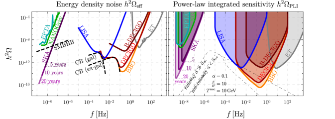
To investigate the detectability of the predicted gravitational wave signals from hidden sector phase transitions, we follow a frequentist approach by calculating the corresponding signal-to-noise ratio (SNR) . A stochastic gravitational wave background is detectable if the signal-to-noise is greater than a certain threshold value , which is either given by the experimental collaborations or extracted from existing data as described in Appendix B.
The optimal-filter cross-correlated signal-to-noise is Thrane:2013oya ; Caprini:2018mtu 444For the case of a single-detector auto-correlated analysis, the factor in Eq. 35 has to be dropped.
| (35) |
where is the duration of the observation, is the detector frequency band, and is the effective noise energy density, i.e. the noise spectrum expressed in the same units as the spectral gravitational wave energy density Thrane:2013oya . See Section B.1 for more details.
To make the comparison between the predicted signal and the noise even simpler, it has become standard practice to quote so-called power-law integrated (PLI) sensitivity curves Thrane:2013oya . They are obtained by assuming the gravitational wave spectrum follows a power law with spectral index , i.e.
| (36) |
where is the gravitational wave energy density at the arbitrarily chosen reference frequency . According to Eq. 35, such a power-law signal is detectable if
| (37) |
The PLI sensitivity curve is then obtained by determining as a function of the spectral index , and quoting the envelope of the corresponding power-law spectra as the sensitivity limit of the experiment. In other words, the PLI sensitivity curve is given by
| (38) |
The region enclosed by the PLI sensitivity curve can be interpreted as the region accessible by the experiment. Pictorially, a gravitational wave spectrum that reaches into this region has a sufficiently large signal-to-noise ratio to be detected. Strictly speaking, this interpretation is only true for spectra that follow a power-law in the frequency band of the detector. However, realistic stochastic gravitational wave backgrounds are at least approximate broken power laws. This means in particular that at the points where the predicted spectrum crosses the sensitivity limit, it is usually well-described locally by a power-law, making the comparison to the PLI sensitivity curve meaningful. Nevertheless we will use Eq. 35 directly to evaluate the detectability of specific sets of model parameters.
The noise levels and PLI sensitivity curves for a number of gravitational wave observatories are shown in Fig. 2. In particular, we consider the proposed ground-based Einstein Telescope (ET) Sathyaprakash:2012jk , the planned space-based LISA Audley:2017drz interferometer as well as the proposed successor experiments BBO Crowder:2005nr and (B-)DECIGO Seto:2001qf ; Sato:2017dkf ). Moreover, we include PTAs, in particular the currently operating EPTA Lentati:2015qwp and NANOGrav (NG) Arzoumanian:2018saf , as well as the future SKA Janssen:2014dka telescope. The data underlying these curves are included in machine-readable form as ancillary material.
II.5 Results
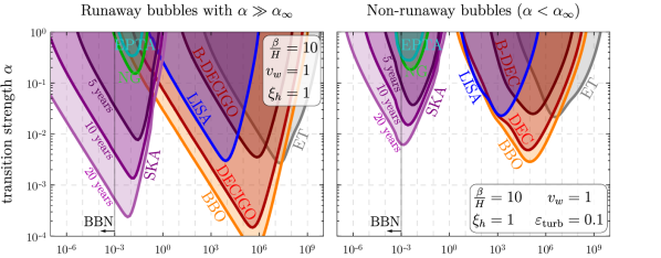
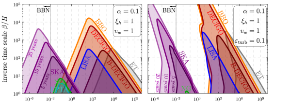
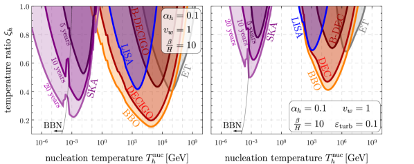
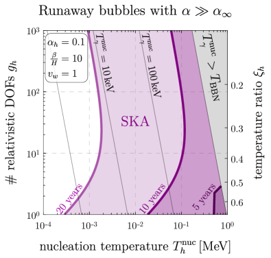
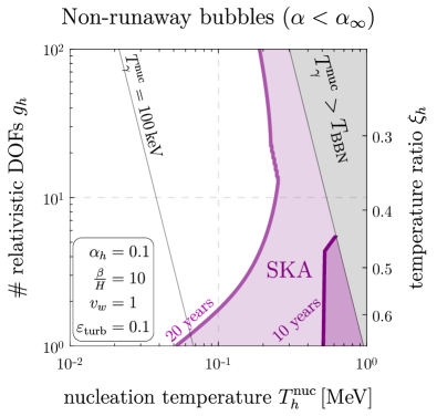
We now translate the noise curves from Fig. 2 (left) into anticipated constraints on the phase transition parameters , , and (introduced in Section II.2) and on the temperature ratio . In Fig. 3, we show the regions where as a function of and (top), and (middle), and and (bottom). The left-hand (right-hand) panel corresponds to runaway (non-runaway) bubble walls. To show the dependence for fixed values of in the bottom panel, we do not fix (which itself depends on ). Instead, we keep the latent heat fixed by fixing the parameter defined as the value of assuming .
The upper panels of Fig. 3 show that PTAs have optimal sensitivity to phase transitions occurring at hidden sector temperatures between and for non-runaway bubbles, with the lower reach increasing far below the scale for runaway bubbles. Ground-based and space-based interferometers will cover the range from to , where again the lower reach increases to the scale for non-runaway bubble walls. As expected, the discovery reach is best for large and small , corresponding to phase transitions that involve highly energetic collisions of large bubbles. The middle right-hand panel of Fig. 3 reveals that the high temperature boundary of the sensitivity curve shifts towards lower temperature scales for increasing . As a consequence, fast phase transitions () will be detectable by pulsar timing only for . A mass spectrum at that scale and below can easily come into conflict with cosmological constraints.
The characteristic kink in the low temperature boundary of the sensitivity curve for versus and non-runaway bubbles (middle right-hand panel of Fig. 3) arises due to the shape of the gravitational wave spectrum. For non-runaway bubbles the spectrum comprises of two contributions (sound wave and turbulence), compared to the single dominant piece for the runaway scenario with . Starting with small at the lower edge of the sensitivity curve, the peak frequency for both contributions lies at frequencies below the lower frequency threshold of the detector. However, due to the large amplitude (), there is nevertheless sensitivity to the high-frequency tail of the turbulence contribution. Increasing decreases the amplitude and increases the peak frequency of both contributions. Thus, the spectral tail of the turbulence contribution drops below the experimental sensitivity, but simultaneously, the peak region of the spectrum (which is dominated by sound waves) moves into the sensitivity region. The kink in the middle right-hand panel of Fig. 3 indicates where the sensitivity changes from being dominated by turbulence to being dominated by sound waves. In contrast, the case of runaway bubbles results in a spectrum dominated by the scalar field contribution, leading to sensitivity curves that are roughly symmetric.
For values of the amplitude of the gravitational wave spectrum arising from sound waves caused by non-runaway bubbles may be overestimated. In this regime the sound wave contributions are expected to last less than a Hubble time, quickly transitioning to turbulent flows in the plasma. This will result in a decrease in amplitude of the gravitational waves sourced from sound waves, but is argued to increase the contribution arising from turbulence Hindmarsh:2017gnf ; Ellis:2018mja . Such an increase is expected to mitigate the overall reduction in the amplitude of the gravitational wave spectrum. Given that this transition between the two regimes cannot yet be accurately simulated, the exact decrease in magnitude remains unknown. Hence, we neglect these dynamics in both Fig. 3 and the model dependent results in the following section.
Comparing the sensitivity to phase transitions with runaway bubbles (left column in Fig. 3) with the sensitivity to non-runaway transitions (right column), we see that in the runaway case, significantly larger regions of parameter space can be probed. The only exception arises for large values of . From Table 1 we observe that the scalar field contribution is suppressed by an extra power of compared to both the sound wave and turbulence contributions.
In the bottom row of Fig. 3, we observe that the sensitivity drops for , which is due to the scaling of the transition strength parameter for fixed (see Eqs. 22 and 23). For small , the photon temperature at the time of the phase transition is much larger, hence the suppression. We emphasize here that for a fixed value of the latent heat (or equivalently for a fixed , the strength of the transition assuming ) a strong phase transition is more easily obtained at later times when the radiation energy density of the universe is lower. This increase is then offset by the effects of the temperature ratio, with the net result being an observable gravitational wave signal for large regions of and .
In Fig. 4 we show the maximum number of degrees of freedom that can be present in a hidden sector whilst being consistent with measurements at BBN and simultaneously producing an observable gravitational wave signal in SKA. This figure is produced assuming the number of degrees of freedom saturates the BBN constraint shown in the left-hand panel of Fig. 1, i.e. we assume that the hidden sector is decoupled from the visible sector and remains so throughout the thermal history. (In the -quilibration scenario, there would be an additional parameter , making visualization difficult.) We see that in the runaway case, SKA may be sensitive to hidden sectors with an number of relativistic degrees of freedom already after 5 years of observation time. Discovery prospects are best for a phase transition at the beginning of BBN. In the non-runaway scenario, at least 10 years of observation time are required to access models with an number of relativistic degrees of freedom. For longer observation periods, the reach will include models with significantly more degrees of freedom within certain temperature ranges. The shape of the sensitivity curves in Fig. 4 can be understood by noting that, even for arbitrarily large , the constraint forces us to keep the total radiation energy density fixed. This implies that a change in is accompanied by a compensating change in . Since we have chosen a fixed and , this means that a larger number of degrees of freedom simply implies that the phase transition happens earlier (), that decreases (see Eq. 22), and that the peak frequency increases (see Table 1). Combining this behavior with the shape of the SKA sensitivity curve from Fig. 2 leads to the sensitivity regions shown in Fig. 4.
We emphasize again that we have here assumed that the stochastic SMBHB background will eventually be resolvable. If this is not the case, the sensitivity regions of SKA shrink almost to the size of the EPTA and NANOGrav regions.
III Models
We now apply the model-independent results from Section II to two specific toy models, which can serve as benchmarks for future studies. We focus on models that feature first-order hidden sector phase transitions at scales and might thus be detectable by PTAs. In addition we focus purely on the hidden sector field content and symmetries, setting potentially allowed portal couplings to the SM exactly to zero. This is motivated by the requirement that any portal coupling present must be sufficiently small555In the case of a scalar portal, forbidding thermal equilibrium through scattering all the way down to the scale requires . to forbid thermal equilibrium between the two sectors. A detailed discussion of concrete realizations yielding a temperature ratio between the two sectors as well as the allowed coupling values that preserve it until the phase transition is given in Ref. Fairbairn:2019xog . Finally, because of the strong constraint, any ultraviolet-complete model with non-trivial dynamics at the MeV scale should reduce to one of a small number of effective low energy models.
III.1 Singlet Scalars
For our first toy model, we consider a hidden sector in which a real scalar singlet acquires a tree-level potential barrier between the two possible minima of its scalar potential. In the most minimalistic setup, such a barrier is generated by the cubic term in the potential. If this coupling is non-zero, and if the mass term is positive, the tree-level potential at zero temperature has one minimum at , and a second one away from the origin. The effective potential at high temperatures, on the other hand, has only a single minimum. This can be seen from both the left-hand panel of Fig. 5 and from the analytical form of the high-temperature expansion (Eq. 51 in Appendix A).666Here and in the following, we denote by an arbitrary value of the field, while we reserve the notation (or, equivalently, ) for the value of the field at its global minimum. The leading term in this effective potential is , where is the field-dependent mass parameter, i.e. the second derivative of the tree-level potential with respect to . From its explicit form given in Eq. 54, we see that is approximately parabolic at high , with a minimum shifted away from the origin. Following the evolution of to lower temperatures, we find that this minimum evolves smoothly into the global minimum of the zero-temperature potential (see left-hand panel of Fig. 5). This means that the field never finds itself in a false vacuum, and no first-order phase transition occurs.
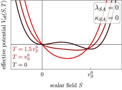
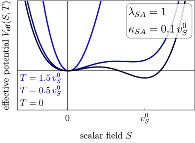
The situation is different if we introduce a second, auxiliary, real singlet scalar . The resulting scalar potential is given by
| (39) |
where we have assumed that is odd under a symmetry. We furthermore assume to avoid spontaneous breaking of the symmetry. The scalar quartic couplings , are required to be positive to ensure stability of the potential. The quartic and trilinear portal terms, and , contribute quadratically and linearly through the thermal potential . These contributions shift the minimum in the -field direction closer to the origin at high temperatures. This enables to first evolve into the false minimum at the origin as the temperature drops, and eventually tunnel into the true minimum in a first-order phase transition (as illustrated in the right panel of Fig. 5). In particular, an analysis of the tree-level potential implies that such a transition occurs if
| (40) |
where is the vacuum expectation value (vev) of at zero temperature. In the following, we will treat as an input parameter of the model and solve the extremal condition to determine .
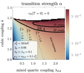
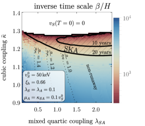
Figure 6 shows the resulting gravitational wave parameters and in the – plane at . To obtain these plots, we have simulated the phase transition using the CosmoTransitions package Wainwright:2011kj ; Kozaczuk:2014kva ; Blinov:2015sna ; Kozaczuk:2015owa , which we have extended to compute gravitational wave parameters and to improve the stability and performance during parameter scans. The actual gravitational wave spectra were then taken from the hydrodynamic simulations discussed and referenced in Section II.3.777As we are including both the sound wave and turbulence contributions to the gravitational wave spectrum, the results here rely on bubble nucleation occurring in a plasma. However, in contrast to the SM plasma, before and after the phase transition there are no completely massless degrees of freedom in the model. Nevertheless, the hierarchy of the mass spectrum in relation to the nucleation temperature ensures that there remains at least one relativistic degree of freedom and therefore a plasma in the broken phase of the hidden sector. The time frame before these relativistic degrees of freedom become non-relativistic is sufficient for the sound wave contributions to source gravitational waves as the scenarios considered here have large values and negligible supercooling. A similar picture holds for the dark photon model considered in the following section. Details on the computation of the effective potential that is used as an input for CosmoTransitions are given in Appendix A. A first-order transition occurs only in the shaded regions of parameter space. The parameters and are the most important handles controlling the dynamics of the phase transition. As already mentioned, (or a combination of and in the case of a non-zero cubic) is required to trap the high-temperature vacuum in a local minimum. This explains why increasing opens up more parameter space in which a first-order transition occurs. on the other hand controls the size of the potential barrier between the true and false vacua. The transition becomes slower and more energetic as is increased. Above a certain threshold, however, the nucleation criterion in Eq. 21 is never met (i.e. the tunneling action never drops below the threshold value required for the transition to begin). In this case, the field remains trapped in the false minimum with . The upper bound on quoted above is at tree level, however this upper bound is further reduced when radiative and temperature-dependent corrections are included. Note also that the bubbles of the phase transitions in the parameter region of interest are close to the boundary between runaway and non-runaway regime, i.e. , as indicated by the dotted lines in Fig. 6.
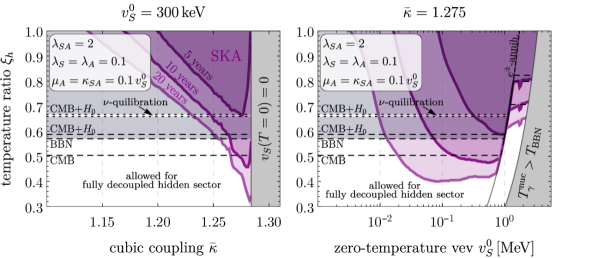
In Fig. 7 we show the expected sensitivity of SKA to the gravitational wave signal from the phase transition in the scalar singlet model. We vary and , while keeping all dimensionless couplings fixed at values, as indicated in the plots. We choose the remaining dimensionful parameters and such that is heavier than while their zero-temperature masses are both of order . This is a requirement of the -equilibration scenario such that doesn’t remain as a stable thermal relic, while the lighter field decays to SM neutrinos. A concrete incarnation of this mechanism is discussed at the end of this subsection. We vary the temperature ratio between the visible and hidden sector at the time of the phase transition (vertical axis), indicating which parameter regions are allowed by cosmological bounds on (white areas). If the hidden sector remains decoupled throughout the post-BBN evolution of the Universe, , or is required by the CMB, CMB+ and BBN constraint given in Eq. 3, Eq. 4 and Eq. 5 respectively. If the hidden sector equilibrates with neutrinos before the phase transition, then the temperature ratio during the phase transition is . The boundaries of the corresponding narrow white band are determined by varying the initial temperature ratio before (re-)coupling between and the maximum possible value from the CMB bound of Fig. 1.
In this context, let us comment on possible mechanisms to realize -quilibration. One possibility is to introduce a small Yukawa-like coupling between and the light neutrinos Berlin:2017ftj ; Berlin:2018ztp , for instance via a right-handed neutrino, , with an interaction term of the form . The assumption of a type-I seesaw then yields a suppressed coupling of the desired form , where is a light neutrino field after electroweak symmetry breaking, and and are the masses of the light and heavy neutrinos, respectively. While both and the neutrinos are relativistic, the interaction rate between the hidden and visible sectors scales proportional to , i.e. it drops more slowly than the Hubble rate (where is the Planck mass). Therefore, it will be initially smaller than , but may become larger at late times, post-BBN. Once the hidden sector particles become non-relativistic, their annihilation back to SM neutrinos can also efficiently proceed as the lightest hidden sector particle, , now has a decay mode to SM neutrinos.
III.2 Dark Photon
As a second toy model, we consider a scenario with an Abelian gauge symmetry in the hidden sector. Gravitational wave signatures arising from gauge symmetries broken at temperatures above the MeV-scale have been considered before as part of a hidden sector Hashino:2018zsi ; Addazi:2017gpt , or as a thermally coupled extension of the SM gauge symmetries Madge:2018gfl . Here, we focus instead on phase transitions at temperatures below . We introduce a complex scalar , which is a singlet under the SM gauge groups, but charged under . The relevant terms in the Lagrangian are
| (41) |
where and are the field strength tensors of and , respectively, and is the SM Higgs field. The covariant derivative acting on is
| (42) |
where is the coupling strength and is the gauge boson of . The most generic renormalizable scalar potential invariant under the model’s symmetries is given by
| (43) |
We see that the hidden and visible sectors can communicate with each other through two portals: the kinetic mixing term between gauge bosons, and the mixed quartic (“Higgs portal”) coupling in the scalar potential. For our purposes, we will assume that the dark sector is sequestered from the visible sector, i.e. we set .
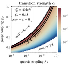
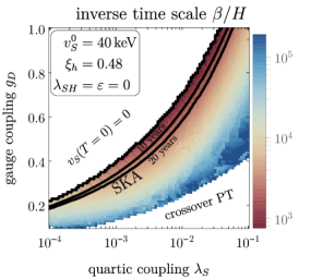
Figure 8 shows our numerical results for the gravitational wave parameters and in the – plane at . Similar to in the singlet scalar model, controls the size of the potential barrier in this case. However, the barrier-inducing cubic term in the effective potential is now a one-loop effect rather than tree level (see Appendix A for details). For increasing values of , the transition becomes slower and more energetic, until becomes too large and the scalar vev remains trapped at . In the opposite limit of small , the transition becomes weaker and faster before entering the regime of smooth crossover transitions without gravitational wave emission. With increasing , the region in which a first-order transition occurs deforms towards higher values of . This is because, for fixed , the parameter which controls the depth of the potential in the broken minimum is proportional to . As a consequence, a deeper tree-level minimum (larger ) has to be paired with a larger barrier (larger ) in order to leave the dynamics of the transition qualitatively unchanged. The tree-level masses of the scalar and the dark photon in the investigated parameter region are with being lighter than because of the parameter choice , . Note that due to the additional friction induced by the dark photon we assume non-runaway bubble walls in the phase transition of this model Bodeker:2017cim .
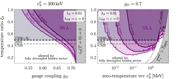
As for the singlet scalar model, we have also computed the sensitivity of SKA to the parameter space of the dark photon model as a function of the temperature ratio . The results are shown in Fig. 9. Due to the additional degrees of freedom in the dark photon model compared to the singlet scalars model, the scenario in which the hidden sector equilibrates with the neutrinos (-quilibration) is completely excluded by the CMB constraints on (see Fig. 1). The white region indicates the allowed temperature ratios for a hidden sector that remains decoupled, corresponding to , and corresponding to the CMB, CMB+ and BBN constraints given in Eq. 3, Eq. 4 and Eq. 5 respectively.
III.3 Random Parameter Scans
Thus far we have shown only specific cuts through the parameter space of our toy models. To better illustrate the full range of parameters that yields observable signals we plot in Fig. 10 the results of random parameter scans for both our toy models, overlaid with the sensitivities of different future gravitational wave observatories. For the singlet scalar model, we have chosen the parameter ranges as follows: , , . Note that the quartic couplings and play only a negligible role for the dynamics of the phase transition. For the dark photon model we scan over , . To produce the plots in Fig. 10, we have first determined the parameters (i.e. the value of assuming ) and for 4 000 random parameter points per model while keeping the value of fixed. Next, we have rescaled the resulting gravitational wave parameters such that all random points have the same nucleation temperature (indicated in the plots). This rescaling affects due to the temperature dependence of , and through the temperature dependence of the nucleation condition. Finally, we have rescaled according to Eqs. 22 and 23 to the desired temperature ratio while keeping fixed.
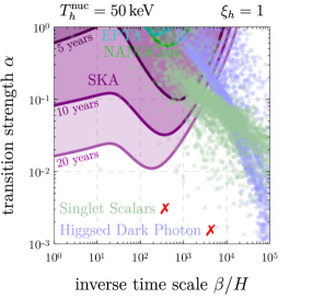
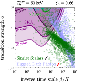
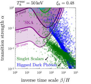
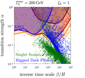
The resulting random points are displayed in Fig. 10 together with the experimental sensitivities (shaded regions), i.e. the regions where the signal-to-noise ratio in a given gravitational wave observatory exceeds the detection threshold. For the determination of these regions, the temperature ratio enters again as it alters the redshift of the signal amplitude and peak frequency, see Eq. 28. Figure 10 reveals that the singlet scalar model features transitions that tend to be weaker (smaller ) compared to the Higgsed dark photon model in most of the considered parameter space. Typically, there exists a limit to how large the barrier between the true and false vacuum can be without forcing the Universe into the true vacuum already at high temperatures. This places a lower limit on the size of . We also observe that the correlation in the – plane is more pronounced for the dark photon model than for the singlet scalar model. This is related to the fact that in the dark photon model, the dynamics of the phase transition has a significant dependence on only two of the particle physics parameters ( and ), while in the singlet scalars model, there is a dependence on five parameters. At a nucleation temperature of , SKA will be sensitive to a significant portion of the parameter space for both models, while EPTA and NANOGrav would only able to exclude a few extreme points. At this scale, however, a temperature ratio is required to ensure a consistent cosmology. For (upper-right panel in Fig. 10) the singlet scalar model is allowed in the -quilibration scenario if the less stringent CMB constraint from Eq. 4 is applied. When assuming a fully decoupled and even colder hidden sector, with (lower-left panel), both models are allowed by the CMB+ and BBN constraints. At (bottom-right panel), the latent heat released in the phase transition, measured in units of to the total energy density of the Universe, is much smaller than at . This results in values for that are more than an order of magnitude smaller for otherwise identical model parameters. Therefore, at , only the far-future space-based interferometers DECIGO and BBO would be sensitive to the Higgsed dark photon model, while LISA and B-DECIGO cover only very small portions of its parameter spaces. Meanwhile, the transitions of the singlet scalar model turn out to be mostly undetectable for .
Comparing the situation for a dark sector at the same temperature as the photons (, upper-left of Fig. 10) with the situation for a cooler dark sector ( in the upper-right panel and in the lower-left panel), we see that the associated rescaling of moves many parameter points outside the detectable window. Nevertheless, a non-negligible fraction of points remains detectable for phase transitions at low .
We conclude that, in our toy models, a stochastic gravitational wave background from a phase transition in the early Universe can be observed only if the nucleation temperature is low (typically in the range – for the large exhibited) and the dark sector is significantly colder than the visible sector (to avoid CMB and BBN constraints), or if we wait for far-future observatories like DECIGO or BBO.
IV Conclusions
In summary, we have studied gravitational wave signals from first-order cosmological phase transitions, in particular transitions occurring in a secluded hidden sector. We have paid special attention to phase transitions at low (sub-MeV) temperatures. Secluded hidden sectors at such low scales cannot be explored using traditional approaches such as collider searches or direct dark matter searches. The main constraints instead arise from cosmological measurements of the relativistic energy density, parameterized by . Taking these constraints into account, we have first restricted the number of hidden sector degrees of freedom as a function of the hidden sector temperature, see Fig. 1.
As expected, hidden sectors with non-trivial dynamics below are only allowed if they are colder than the Standard Model sector by an factor. We have then investigated the detectability of gravitational wave signals from such a light hidden sector, focusing in particular on the sensitivity of pulsar timing arrays, which are the most relevant experiments for such low-frequency signals. Noise curves and power law-integrated sensitivity curves for a range of experiments are given in Fig. 2, and the data underlying this figure is attached as ancillary material. We have found that detectable signals are only expected if the hidden sector is not too much colder than the Standard Model sector, see for example the bottom row of Fig. 3. These requirements on the hidden sector temperature allow us to bound the parameter range in which observable gravitational wave signals can occur from both directions. The results of which are shown in Fig. 4.
We have also considered phase transitions at higher temperatures, where hardly any cosmological constraints exist. However, at high temperatures, the gravitational wave energy density is typically much smaller compared to the total energy density of the Universe, making the transition strength parameter small and the signal more challenging to detect.
We have finally corroborated the above statements by constructing two specific toy models featuring phase transitions at sub-MeV temperatures: one with just an extended scalar sector, and one with a Higgsed gauge symmetry in the hidden sector. Because of the above constraints on the number of hidden sector degrees of freedom and on their temperature, we expect that many models with observable low-temperature phase transitions reduce to one of our toy models, or a model very similar to them, at low energies. Thus, our toy models offer interesting discovery opportunities for SKA in a range of gravitational wave frequencies inaccessible to any other observatory.
Acknowledgments
TO would like to thank Stefan Huber and Jose Miguel No for enlightening discussions. TO is also grateful to CERN for hospitality and support during crucial stages of this project. The authors have received funding from the German Research Foundation (DFG) under Grant Nos. EXC-1098, FOR 2239, GRK 1581 and KO4820/4-1, and from the European Research Council (ERC) under the European Union’s Horizon 2020 research and innovation programme (grant agreement No. 637506, “Directions”).
Appendix A The Effective Potential
A.1 General Formalism
A central ingredient in our analysis of the cosmological evolution of the toy models from Section III is the finite-temperature effective potential
| (44) |
evaluated at one-loop in the perturbative expansion.888Note that, in general, depends on all scalar fields in the model. In our toy models however, we only care about the dependence on : in the singlet scalar model, the auxiliary scalar never acquires a vev; in both models, couplings between the hidden sector scalars and the SM Higgs field are assumed to be tiny. Here, is the tree-level potential. The one-loop contribution splits up into a ultraviolet-divergent zero-temperature (Coleman–Weinberg) part, , and a finite-temperature part, . We also include the resummed contribution from ring diagrams, .
The renormalized Coleman–Weinberg part is given by Coleman:1973jx ; Quiros:1999jp ; Laine:2016hma
| (45) |
where runs over all particle species with -dependent mass, is the number of degrees of freedom for each species, and () for bosons (fermions).999Since we are working in Landau gauge, the sums in this section are meant to include both the Goldstone bosons and the longitudinal gauge boson modes. Despite the Goldstone boson equivalence theorem this does not imply double counting, as demonstrated in Delaunay:2007wb . For the renormalization scale , we choose the tree-level vev . Ultraviolet divergences are canceled by counter-terms, while the remaining finite parts of the counter-terms are subsumed in . The constant () for scalars and fermions (gauge bosons) is an artifact of dimensional regularization. We write the finite part of the counter-terms as
| (46) |
in the singlet scalar model from Section III.1, and as
| (47) |
for the dark photon model from Section III.2. We determine the counter-term couplings by imposing the renormalization conditions
| (48) | ||||
which fix the zero-temperature vev and mass to their tree-level values. For the singlet scalar model, we additionally want to fix the structure of the minima, which is approximately achieved by requiring
| (49) |
The finite-temperature part of the one-loop potential evaluates to Dolan:1973qd ; Quiros:1999jp ; Laine:2016hma
| (50) |
At high temperature, this expression can be expanded as Laine:2016hma
| (51) | ||||
where we have included only the leading field dependent pieces.
In addition to the one-loop contributions to , we also consider the ring diagram (“daisy”) contributions, which read Carrington:1991hz ; Quiros:1999jp ; Delaunay:2007wb
| (52) |
after resumming an infinite series of infrared-divergent diagrams. Here, denotes the temperature dependent Debye mass, which vanishes for transverse gauge boson modes Carrington:1991hz . In the above formula, has to be interpreted as the -th eigenvalue of the full (tree-level + thermal) mass matrix Patel:2011th . Here we note that the cubic terms exactly cancel between the high-temperature expansions of and . Coupling one or more gauge bosons to a scalar field is therefore a possibility to generate a loop-induced barrier, rendering the phase transition first-order. This is based on the fact that the cancellation of cubic terms occurs only for longitudinal polarizations, but not for the transverse polarizations. We utilize this barrier formed by the transverse polarization to induce a first-order phase transition in the Higgsed dark photon model of Section III.2.
A.2 Model Details
In the following, we list the scalar-field dependent particle masses, thermal Debye masses, and tree-level minimization conditions for the two toy models from Section III. These parameters need to be plugged into the equations from Section A.1 to compute the effective potential .
In the singlet scalar model, the tree-level minimization condition for the scalar potential is
| (53) |
The field-dependent scalar masses of and are
| (54) | ||||
| (55) |
and their Debye masses are
| (56) | ||||
| (57) |
In the Higgsed dark photon model, the scalar potential is at its tree-level minimum when
| (58) |
The field-dependent masses of the two scalar degrees of freedom and of the dark photon are
| (59) | ||||
| (60) | ||||
| (61) |
Note that, at the minimum of the potential (), corresponds to the massive scalar degree of freedom, while is the Goldstone mode, as can be easily seen from Eq. 58. The Debye masses are
| (62) | ||||
| (63) |
Appendix B Sensitivity Curves
In the following, we explain in detail how the experimental sensitivity curves discussed in Section II.4 (see for instance Fig. 2) have been obtained.
B.1 Signal-to-Noise Ratio
Consider a system of gravitational wave detectors with output
| (64) |
where is the strain induced by the gravitational wave signal we are looking for and is the noise in detector . (Both quantities are assumed to be already convoluted with the detector response function, see e.g. Ref. Thrane:2013oya .) One can then define a (pair-wise) cross-correlated signal observed over a long time interval by
| (65) |
where is a filter function. The filter function will be chosen such that it maximizes the signal-to-noise ratio
| (66) |
where denotes an ensemble average, realized either by integrating over different spatial regions or by integrating over many observations, each of duration . In the following, it is convenient to work with the Fourier transforms of , , , and , which are defined as usual by
| (67) | ||||
| (68) |
and similar expressions for and . Assuming that the gravitational wave background and the noise are Gaussian and stationary, and that the noise levels in the individual detectors are statistically independent, one can define the power spectral densities and via Allen:1997ad ; Thrane:2013oya ; Caprini:2018mtu
| (69) | ||||
| and | ||||
| (70) | ||||
Here, is called the overlap reduction function. It encodes the sky-averaged and polarization-averaged detector response to an incoming gravitational wave, taking into account the reduction in sensitivity due to different locations and orientations of the two detectors and . Note that, for the noise, we use a quantity defined directly in terms of the detector response, whereas for the signal, it is more convenient to work with , which has detector effects () factored out. is related to the fractional cosmological gravitational wave energy density spectrum (see Section II.3) via
| (71) |
With these definitions, and with the optimally chosen
| (72) |
(see for instance Caprini:2018mtu ), the signal-to-noise-ratio from Eq. 66 can be rewritten as
| (73) |
Here, and are the bounds of the frequency region to which the detectors are sensitive. Frequencies outside this region do not contribute to the signal-to-noise ratio. It is finally convenient to define the noise energy density spectrum of the detector network as
| (74) |
With this definition, we can bring the signal-to-noise ratio to its final form Thrane:2013oya ; Caprini:2018mtu
| (75) |
This is just Eq. 35.
Given the effective noise curve and the threshold value , we can now evaluate whether a given stochastic gravitational wave background can be detected.101010Note, however, that in obtaining Eq. 75, the filter function has been optimized for the expected gravitational wave signal, requiring a priori knowledge of this signal. Thus, when dealing with real data, the analysis would have to be repeated for each type of signal to be tested against. This is typically not feasible, therefore, the sensitivity obtained in this way should be regarded as only an estimate.
B.2 Pulsar Timing Arrays
| Experiment | Reference | |||||
|---|---|---|---|---|---|---|
| EPTA | Lentati:2015qwp ; Desvignes:2016yex | |||||
| NANOGrav | Arzoumanian:2018saf | |||||
| SKA | , , | 4 | Bull:2018lat ; Janssen:2014dka (assumptions) |
PTA limits on a stochastic gravitational wave background are usually quoted in terms of the minimal detectable amplitude of the characteristic strain
| (76) |
which we parameterize as a simple power-law, i.e.
| (77) |
Here, is the strain amplitude at an arbitrary reference frequency which we choose as . The background in a PTA is typically assumed to be generated by unresolved supermassive black hole binary (SMBHB) systems, in which case , or by cosmic strings with Lentati:2015qwp ; Arzoumanian:2018saf ; Caprini:2018mtu . The corresponding gravitational wave power spectrum is related to the strain by Thrane:2013oya ; Moore:2014lga
| (78) |
with (see also Eq. 36).
We consider here current constraints from the observation of pulsars over a time span of 18 years by EPTA Lentati:2015qwp and over 11 years from NANOGrav Arzoumanian:2018saf , as well as prospective limits from SKA Janssen:2014dka . EPTA and NANOGrav present their results as limits on the gravitational wave amplitude as a function of frequency for a spectrum with freely-varying spectral index obtained using a Bayesian approach. We use these curves as an estimate for and take the signal-to-noise threshold equal to the signal-to-noise that saturates the limits on the SMBHB background (). These limits are for NANOGrav Arzoumanian:2018saf and for EPTA Lentati:2015qwp , which leads to for EPTA with and for NANOGrav with .
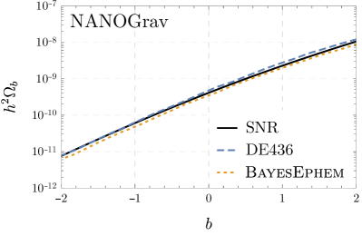
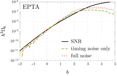
As a cross-check we have used these values in Eq. 75 to compute the limits on the gravitational wave amplitude at as a function of the spectral slope. In Fig. 11, we compare these limits to the bounds derived by the collaborations. We see that for spectral slopes , our limits agree very well with the ones provided by the collaborations. For larger , the official EPTA limits are somewhat stronger than our estimates. (NANOGrav does not show limits in this range.)
For the sensitivity of SKA, we work in the weak signal limit where the noise is the dominant contribution to the detector output (this is particularly good assumption when timing a large number of pulsars). In addition we assume that the timing-residual noise of each pulsar is white, Gaussian and uncorrelated. The noise power spectral density can then be written as Thrane:2013oya ; Moore:2014eua
| (79) |
where is the inverse of the pulsar’s cadence (which specifies how frequently the pulsar’s timing residual is measured) and is the residual root-mean-square (rms) error on each of these measurements. We assume white noise, i.e. there is no frequency dependence in . For an array of pulsars randomly distributed over the sky and with equal timing cadence and noise, the effective noise power spectral density then becomes Moore:2014eua
| (80) |
(Note that, by considering the ratio here, we deconvolute the detector response, i.e. can be directly compared to the signal power spectral density .) For our numerical calculations, we approximate as Moore:2014eua
| (81) |
which leads to
| (82) |
In analogy to Eqs. 76 and 78, can be related to a characteristic strain Moore:2014eua ; Moore:2014lga , and thus to an effective energy density spectrum (normalized to the critical density of the Universe),
| (83) |
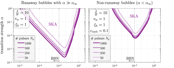
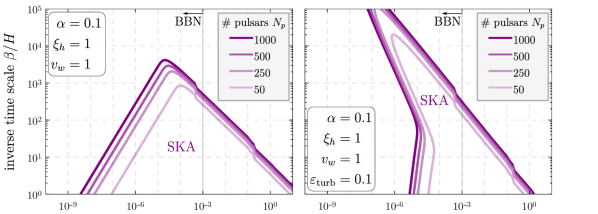
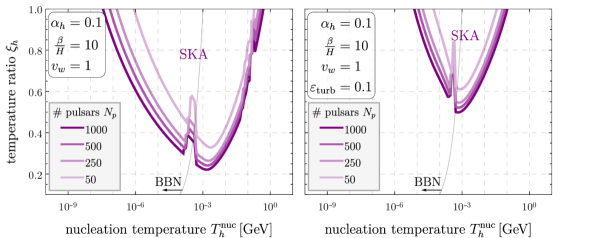
This quantity can then be used in Eq. 75 to determine the signal-to-noise ratio. The integration limits in Eq. 75 should be taken as and Moore:2014lga . Using Eqs. 83 and 75, it is straightforward to rescale the noise and sensitivity curves in Fig. 2 to the actual experimental parameters of SKA once these are known. Nevertheless, in Fig. 12 we show the changes in sensitivity to the gravitational wave parameters when varying the number of pulsars timed. Note that reducing the number of pulsars can affect the validity of the weak signal approximation. Timing around 50 pulsars over an observation run of 20 years yields already percent level deviations between the signal-to-noise defined using Eq. 83, and the full result (relaxing the assumption of a weak signal) in Eq. (19) of Ref. Siemens:2013zla .
As a cross-check we have considered the hypothetical SKA campaign taken from Ref. Janssen:2014dka , which is based on pulsars timed once per week () over a time span of . The residual noise has been assumed to be , and the detection threshold has been taken as . Plugging these numbers into Eq. 83 for the noise and Eq. 78 for the signal (with for a stochastic gravitational wave signal due to SMBHBs), and using the result in Eq. 75 for the signal-to-noise ratio, we find that the minimal detectable energy density for a SMBHB signal is at a frequency of . Converted into a characteristic strain this gives , which agrees with the estimate – from Ref. Janssen:2014dka . (Note that in the analyses presented in the main part of the paper, we consider a more optimistic SKA configuration, as given in Table 2 based upon the feasibility study of Ref. Bull:2018lat .)
B.3 Space-Based Interferometers
In this work we consider the projected sensitivities for the LISA experiment Audley:2017drz , which is planned to be launched in 2034 Caprini:2018mtu , as well as the proposed successor experiments BBO Crowder:2005nr , B-DECIGO Sathyaprakash:2012jk , and DECIGO Seto:2001qf .
While DECIGO and BBO will consist of networks of gravitational wave detectors, LISA and B-DECIGO are single-detector observatories. Hence, the cross-correlation analysis that has led to Eq. 75 is not directly applicable to LISA and B-DECIGO. Instead, we need to use the auto-correlated signal-to-noise
| (84) |
This expression differs from Eq. 75 by just a factor of two and is thus equal to the squared cross-correlated signal-to-noise for a pair of detectors divided by two, since we only use one detector.
For LISA we assume a mission duration of Audley:2017drz and an signal-to-noise detection threshold of Caprini:2015zlo . We use the noise strain power spectral density quoted in Ref. Cornish:2018dyw to be
| (85) |
where is LISA’s interferometer arm length and is called the transfer frequency where is the speed of light. The instrument noise is composed of the optical metrology noise
| (86) |
and the test mass acceleration noise
| (87) |
The confusion noise from unresolved galactic binaries after 4 years is
| (88) |
For B-DECIGO (the scaled-down predecessor of DECIGO, with a planned launch in the late 2020’s Sato:2017dkf ), the effective noise strain power spectral density is Isoyama:2018rjb
| (89) |
(Note that we include an additional factor compared to Ref. Isoyama:2018rjb to account for sky-averaging.) The frequency range for B-DECIGO is , , the detection threshold is , and the assumed observation time is 4 years.
| Experiment | Frequency range | Comment | ||
|---|---|---|---|---|
| LISA | Audley:2017drz | Caprini:2015zlo | Cornish:2018dyw | Eq. 84 for SNR |
| B-DECIGO | Isoyama:2018rjb | Isoyama:2018rjb | Isoyama:2018rjb | for sky-average and Eq. 84 for SNR |
| DECIGO | Yagi:2013du | Yagi:2013du | for sky-average | |
| BBO | Yagi:2011yu | Yagi:2011yu | for sky-average | |
| ET | Sathyaprakash:2012jk | Sathyaprakash:2012jk | Sathyaprakash:2012jk | Eq. 84 for SNR |
The noise curves for the far-future projects BBO Crowder:2005nr and DECIGO Sato:2017dkf can be parameterized as Yagi:2011yu ; Yagi:2013du
| (90) |
where , and is the spectral number density of galactic white dwarf binaries. The non-sky-averaged instrumental noise curves are
| (91) |
with for DECIGO, and
| (92) |
for BBO. The confusion noise from galactic () and extra-galactic () white dwarf binaries is given by
| (93) | ||||
| (94) |
As for LISA, we use an observation time of and a detection threshold of . The frequency range covered by DECIGO and BBO will be from to . Our parameter choices for future gravitational wave interferometers are also summarized in Table 3.
B.4 Earth-Based Interferometers
Due to seismic noise the sensitivity of current ground-based gravitational wave observatories is not sufficient to constrain stochastic backgrounds generated by cosmological phase transitions. However, the next-generation of detectors is going to provide a significant improvement in sensitivity.
We hence include sensitivity projections for the third-generation observatory ET Yagi:2011yu ; Yagi:2013du . We employ the ET-D noise projections Hild:2010id , assuming an observation period of 5 years and considering a stochastic background as detectable if it produces an signal-to-noise of 5 in a single ET detector Sathyaprakash:2012jk .
References
- (1) E. Witten, Cosmic Separation of Phases, Phys. Rev. D30 (1984) 272–285.
- (2) C. J. Hogan, Nulceation of Cosmological Phase Transitions, Phys. Lett. 133B (1983) 172–176.
- (3) C. J. Hogan, Gravitational radiation from cosmological phase transitions, Mon. Not. Roy. Astron. Soc. 218 (1986) 629–636.
- (4) M. S. Turner and F. Wilczek, Relic gravitational waves and extended inflation, Phys. Rev. Lett. 65 (1990) 3080–3083.
- (5) C. Caprini et al., Science with the space-based interferometer eLISA. II: Gravitational waves from cosmological phase transitions, JCAP 1604 (2016), no. 04 001, [arXiv:1512.06239].
- (6) C. Caprini and D. G. Figueroa, Cosmological Backgrounds of Gravitational Waves, [arXiv:1801.04268].
- (7) A. Mazumdar and G. White, Cosmic phase transitions: their applications and experimental signatures, [arXiv:1811.01948].
- (8) P. Schwaller, Gravitational Waves from a Dark Phase Transition, Phys. Rev. Lett. 115 (2015), no. 18 181101, [arXiv:1504.07263].
- (9) J. Jaeckel, V. V. Khoze, and M. Spannowsky, Hearing the smoke of dark sectors with gravitational wave detectors, [arXiv:1602.03901].
- (10) A. Addazi, Limiting First Order Phase Transitions in Dark Gauge Sectors from Gravitational Waves experiments, Mod. Phys. Lett. A32 (2017), no. 08 1750049, [arXiv:1607.08057].
- (11) I. Baldes, Gravitational waves from the asymmetric-dark-matter generating phase transition, JCAP 1705 (2017), no. 05 028, [arXiv:1702.02117].
- (12) A. Addazi and A. Marciano, Gravitational waves from dark first order phase transitions and dark photons, Chin. Phys. C42 (2018), no. 2 023107, [arXiv:1703.03248].
- (13) K. Tsumura, M. Yamada, and Y. Yamaguchi, Gravitational wave from dark sector with dark pion, JCAP 1707 (2017), no. 07 044, [arXiv:1704.00219].
- (14) M. Aoki, H. Goto, and J. Kubo, Gravitational Waves from Hidden QCD Phase Transition, Phys. Rev. D96 (2017), no. 7 075045, [arXiv:1709.07572].
- (15) M. Geller, A. Hook, R. Sundrum, and Y. Tsai, Primordial Anisotropies in the Gravitational Wave Background from Cosmological Phase Transitions, [arXiv:1803.10780].
- (16) D. Croon, V. Sanz, and G. White, Model Discrimination in Gravitational Wave spectra from Dark Phase Transitions, JHEP 08 (2018) 203, [arXiv:1806.02332].
- (17) I. Baldes and C. Garcia-Cely, Strong gravitational radiation from a simple dark matter model, [arXiv:1809.01198].
- (18) E. Aver, K. A. Olive, and E. D. Skillman, The effects of He I 10830 on helium abundance determinations, JCAP 1507 (2015), no. 07 011, [arXiv:1503.08146].
- (19) A. Peimbert, M. Peimbert, and V. Luridiana, The primordial helium abundance and the number of neutrino families, Rev. Mex. Astron. Astrofis. 52 (2016) 419, [arXiv:1608.02062].
- (20) Planck Collaboration, P. A. R. Ade et al., Planck 2015 results. XIII. Cosmological parameters, Astron. Astrophys. 594 (2016) A13, [arXiv:1502.01589].
- (21) Planck Collaboration, N. Aghanim et al., Planck 2018 results. VI. Cosmological parameters, [arXiv:1807.06209].
- (22) G. Mangano, G. Miele, S. Pastor, T. Pinto, O. Pisanti, and P. D. Serpico, Relic neutrino decoupling including flavor oscillations, Nucl. Phys. B729 (2005) 221–234, [hep-ph/0506164].
- (23) A. G. Riess, S. Casertano, W. Yuan, L. Macri, J. Anderson, J. W. MacKenty, J. B. Bowers, K. I. Clubb, A. V. Filippenko, D. O. Jones, and B. E. Tucker, New parallaxes of galactic cepheids from spatially scanning the hubble space telescope : Implications for the hubble constant, The Astrophysical Journal 855 (2018), no. 2 136.
- (24) V. F. Shvartsman, Density of relict particles with zero rest mass in the universe, Pisma Zh. Eksp. Teor. Fiz. 9 (1969) 315–317. [JETP Lett.9,184(1969)].
- (25) G. Steigman, D. N. Schramm, and J. E. Gunn, Cosmological Limits to the Number of Massive Leptons, Phys. Lett. B66 (1977) 202–204. [159(1977)].
- (26) R. J. Scherrer and M. S. Turner, Primordial Nucleosynthesis with Decaying Particles. 1. Entropy Producing Decays. 2. Inert Decays, Astrophys. J. 331 (1988) 19–32. [Astrophys. J.331,33(1988)].
- (27) Particle Data Group Collaboration, C. Patrignani et al., Review of Particle Physics, Chin. Phys. C40 (2016), no. 10 100001.
- (28) M. Hufnagel, K. Schmidt-Hoberg, and S. Wild, BBN constraints on MeV-scale dark sectors. Part I. Sterile decays, JCAP 1802 (2018) 044, [arXiv:1712.03972].
- (29) D. Baumann, Primordial Cosmology, PoS TASI2017 (2018) 009, [arXiv:1807.03098].
- (30) C. Boehm, M. J. Dolan, and C. McCabe, Increasing Neff with particles in thermal equilibrium with neutrinos, JCAP 1212 (2012) 027, [arXiv:1207.0497].
- (31) A. Berlin and N. Blinov, Thermal Dark Matter Below an MeV, Phys. Rev. Lett. 120 (2018), no. 2 021801, [arXiv:1706.07046].
- (32) A. Berlin and N. Blinov, A Thermal Neutrino Portal to Sub-MeV Dark Matter, [arXiv:1807.04282].
- (33) R. H. Cyburt, B. D. Fields, K. A. Olive, and T.-H. Yeh, Big Bang Nucleosynthesis: 2015, Rev. Mod. Phys. 88 (2016) 015004, [arXiv:1505.01076].
- (34) M. S. Turner, E. J. Weinberg, and L. M. Widrow, Bubble nucleation in first order inflation and other cosmological phase transitions, Phys. Rev. D46 (1992) 2384–2403.
- (35) M. Kamionkowski, A. Kosowsky, and M. S. Turner, Gravitational radiation from first order phase transitions, Phys. Rev. D49 (1994) 2837–2851, [astro-ph/9310044].
- (36) C. Grojean and G. Servant, Gravitational Waves from Phase Transitions at the Electroweak Scale and Beyond, Phys. Rev. D75 (2007) 043507, [hep-ph/0607107].
- (37) S. R. Coleman, The Fate of the False Vacuum. 1. Semiclassical Theory, Phys. Rev. D15 (1977) 2929–2936. [Erratum: Phys. Rev.D16,1248(1977)].
- (38) C. G. Callan, Jr. and S. R. Coleman, The Fate of the False Vacuum. 2. First Quantum Corrections, Phys. Rev. D16 (1977) 1762–1768.
- (39) A. D. Linde, Decay of the False Vacuum at Finite Temperature, Nucl. Phys. B216 (1983) 421.
- (40) J. R. Espinosa, T. Konstandin, J. M. No, and G. Servant, Energy Budget of Cosmological First-order Phase Transitions, JCAP 1006 (2010) 028, [arXiv:1004.4187].
- (41) V. Brdar, A. J. Helmboldt, and J. Kubo, Gravitational Waves from First-Order Phase Transitions: LIGO as a Window to Unexplored Seesaw Scales, [arXiv:1810.12306].
- (42) J. Ellis, M. Lewicki, and J. M. No, On the Maximal Strength of a First-Order Electroweak Phase Transition and its Gravitational Wave Signal, [arXiv:1809.08242].
- (43) T. Prokopec, J. Rezacek, and B. Świeżewska, Gravitational waves from conformal symmetry breaking, [arXiv:1809.11129].
- (44) B. von Harling and G. Servant, QCD-induced Electroweak Phase Transition, JHEP 01 (2018) 159, [arXiv:1711.11554].
- (45) S. Bruggisser, B. Von Harling, O. Matsedonskyi, and G. Servant, Electroweak Phase Transition and Baryogenesis in Composite Higgs Models, [arXiv:1804.07314].
- (46) T. Konstandin and G. Servant, Cosmological Consequences of Nearly Conformal Dynamics at the TeV scale, JCAP 1112 (2011) 009, [arXiv:1104.4791].
- (47) A. Kobakhidze, C. Lagger, A. Manning, and J. Yue, Gravitational waves from a supercooled electroweak phase transition and their detection with pulsar timing arrays, Eur. Phys. J. C77 (2017), no. 8 570, [arXiv:1703.06552].
- (48) S. Iso, P. D. Serpico, and K. Shimada, QCD-Electroweak First-Order Phase Transition in a Supercooled Universe, Phys. Rev. Lett. 119 (2017), no. 14 141301, [arXiv:1704.04955].
- (49) Y. Bai and A. J. Long, Six Flavor Quark Matter, JHEP 06 (2018) 072, [arXiv:1804.10249].
- (50) E. Megías, G. Nardini, and M. Quirós, Cosmological Phase Transitions in Warped Space: Gravitational Waves and Collider Signatures, [arXiv:1806.04877].
- (51) T. Hambye, A. Strumia, and D. Teresi, Super-cool Dark Matter, JHEP 08 (2018) 188, [arXiv:1805.01473].
- (52) L. Randall and G. Servant, Gravitational waves from warped spacetime, JHEP 05 (2007) 054, [hep-ph/0607158].
- (53) D. Bodeker and G. D. Moore, Electroweak Bubble Wall Speed Limit, JCAP 1705 (2017), no. 05 025, [arXiv:1703.08215].
- (54) S. J. Huber and T. Konstandin, Gravitational Wave Production by Collisions: More Bubbles, JCAP 0809 (2008) 022, [arXiv:0806.1828].
- (55) M. Hindmarsh, S. J. Huber, K. Rummukainen, and D. J. Weir, Numerical simulations of acoustically generated gravitational waves at a first order phase transition, Phys. Rev. D92 (2015), no. 12 123009, [arXiv:1504.03291].
- (56) M. Hindmarsh, S. J. Huber, K. Rummukainen, and D. J. Weir, Shape of the acoustic gravitational wave power spectrum from a first order phase transition, Phys. Rev. D96 (2017), no. 10 103520, [arXiv:1704.05871].
- (57) C. Caprini, R. Durrer, and G. Servant, The stochastic gravitational wave background from turbulence and magnetic fields generated by a first-order phase transition, JCAP 0912 (2009) 024, [arXiv:0909.0622].
- (58) D. J. Fixsen, The Temperature of the Cosmic Microwave Background, Astrophys. J. 707 (2009) 916–920, [arXiv:0911.1955].
- (59) J. Simon and S. Burke-Spolaor, Constraints on Black Hole/Host Galaxy Co-evolution and Binary Stalling Using Pulsar Timing Arrays, Astrophys. J. 826 (2016), no. 1 11, [arXiv:1603.06577].
- (60) NANOGRAV Collaboration, Z. Arzoumanian et al., The NANOGrav 11-year Data Set: Pulsar-timing Constraints On The Stochastic Gravitational-wave Background, [arXiv:1801.02617].
- (61) N. Cornish and T. Robson, Galactic binary science with the new LISA design, J. Phys. Conf. Ser. 840 (2017), no. 1 012024, [arXiv:1703.09858].
- (62) N. Cornish and T. Robson, The construction and use of LISA sensitivity curves, [arXiv:1803.01944].
- (63) A. J. Farmer and E. S. Phinney, The gravitational wave background from cosmological compact binaries, Mon. Not. Roy. Astron. Soc. 346 (2003) 1197, [astro-ph/0304393].
- (64) K. Yagi, N. Tanahashi, and T. Tanaka, Probing the size of extra dimension with gravitational wave astronomy, Phys. Rev. D83 (2011) 084036, [arXiv:1101.4997].
- (65) E. Thrane and J. D. Romano, Sensitivity curves for searches for gravitational-wave backgrounds, Phys. Rev. D88 (2013), no. 12 124032, [arXiv:1310.5300].
- (66) B. Sathyaprakash et al., Scientific Objectives of Einstein Telescope, Class. Quant. Grav. 29 (2012) 124013, [arXiv:1206.0331]. [Erratum: Class. Quant. Grav.30,079501(2013)].
- (67) LISA Collaboration, H. Audley et al., Laser Interferometer Space Antenna, [arXiv:1702.00786].
- (68) J. Crowder and N. J. Cornish, Beyond LISA: Exploring future gravitational wave missions, Phys. Rev. D72 (2005) 083005, [gr-qc/0506015].
- (69) N. Seto, S. Kawamura, and T. Nakamura, Possibility of direct measurement of the acceleration of the universe using 0.1-Hz band laser interferometer gravitational wave antenna in space, Phys. Rev. Lett. 87 (2001) 221103, [astro-ph/0108011].
- (70) S. Sato et al., The status of DECIGO, J. Phys. Conf. Ser. 840 (2017), no. 1 012010.
- (71) L. Lentati et al., European Pulsar Timing Array Limits On An Isotropic Stochastic Gravitational-Wave Background, Mon. Not. Roy. Astron. Soc. 453 (2015), no. 3 2576–2598, [arXiv:1504.03692].
- (72) G. Janssen et al., Gravitational wave astronomy with the SKA, PoS AASKA14 (2015) 037, [arXiv:1501.00127].
- (73) M. Fairbairn, E. Hardy, and A. Wickens, Hearing without seeing: gravitational waves from hot and cold hidden sectors, [arXiv:1901.11038].
- (74) C. L. Wainwright, CosmoTransitions: Computing Cosmological Phase Transition Temperatures and Bubble Profiles with Multiple Fields, Comput. Phys. Commun. 183 (2012) 2006–2013, [arXiv:1109.4189].
- (75) J. Kozaczuk, S. Profumo, L. S. Haskins, and C. L. Wainwright, Cosmological Phase Transitions and their Properties in the NMSSM, JHEP 01 (2015) 144, [arXiv:1407.4134].
- (76) N. Blinov, J. Kozaczuk, D. E. Morrissey, and C. Tamarit, Electroweak Baryogenesis from Exotic Electroweak Symmetry Breaking, Phys. Rev. D92 (2015), no. 3 035012, [arXiv:1504.05195].
- (77) J. Kozaczuk, Bubble Expansion and the Viability of Singlet-Driven Electroweak Baryogenesis, JHEP 10 (2015) 135, [arXiv:1506.04741].
- (78) K. Hashino, M. Kakizaki, S. Kanemura, P. Ko, and T. Matsui, Gravitational waves from first order electroweak phase transition in models with the U(1)X gauge symmetry, JHEP 06 (2018) 088, [arXiv:1802.02947].
- (79) E. Madge and P. Schwaller, Leptophilic dark matter from gauged lepton number: Phenomenology and gravitational wave signatures, JHEP 02 (2019) 048, [arXiv:1809.09110].
- (80) S. R. Coleman and E. J. Weinberg, Radiative Corrections as the Origin of Spontaneous Symmetry Breaking, Phys. Rev. D7 (1973) 1888–1910.
- (81) M. Quiros, Finite temperature field theory and phase transitions, in Proceedings, Summer School in High-energy physics and cosmology: Trieste, Italy, June 29-July 17, 1998, pp. 187–259, 1999. [hep-ph/9901312].
- (82) M. Laine and A. Vuorinen, Basics of Thermal Field Theory, Lect. Notes Phys. 925 (2016) pp.1–281, [arXiv:1701.01554].
- (83) C. Delaunay, C. Grojean, and J. D. Wells, Dynamics of Non-renormalizable Electroweak Symmetry Breaking, JHEP 04 (2008) 029, [arXiv:0711.2511].
- (84) L. Dolan and R. Jackiw, Symmetry Behavior at Finite Temperature, Phys. Rev. D9 (1974) 3320–3341.
- (85) M. E. Carrington, The Effective potential at finite temperature in the Standard Model, Phys. Rev. D45 (1992) 2933–2944.
- (86) H. H. Patel and M. J. Ramsey-Musolf, Baryon Washout, Electroweak Phase Transition, and Perturbation Theory, JHEP 07 (2011) 029, [arXiv:1101.4665].
- (87) B. Allen and J. D. Romano, Detecting a stochastic background of gravitational radiation: Signal processing strategies and sensitivities, Phys. Rev. D59 (1999) 102001, [gr-qc/9710117].
- (88) G. Desvignes et al., High-precision timing of 42 millisecond pulsars with the European Pulsar Timing Array, Mon. Not. Roy. Astron. Soc. 458 (2016), no. 3 3341–3380, [arXiv:1602.08511].
- (89) P. Bull et al., Fundamental Physics with the Square Kilometer Array, [arXiv:1810.02680].
- (90) C. J. Moore, R. H. Cole, and C. P. L. Berry, Gravitational-wave sensitivity curves, Class. Quant. Grav. 32 (2015), no. 1 015014, [arXiv:1408.0740].
- (91) C. J. Moore, S. R. Taylor, and J. R. Gair, Estimating the sensitivity of pulsar timing arrays, Class. Quant. Grav. 32 (2015), no. 5 055004, [arXiv:1406.5199].
- (92) X. Siemens, J. Ellis, F. Jenet, and J. D. Romano, The stochastic background: scaling laws and time to detection for pulsar timing arrays, Class. Quant. Grav. 30 (2013) 224015, [arXiv:1305.3196].
- (93) S. Isoyama, H. Nakano, and T. Nakamura, Multiband Gravitational-Wave Astronomy: Observing binary inspirals with a decihertz detector, B-DECIGO, [arXiv:1802.06977].
- (94) K. Yagi, Scientific Potential of DECIGO Pathfinder and Testing GR with Space-Borne Gravitational Wave Interferometers, Int. J. Mod. Phys. D22 (2013) 1341013, [arXiv:1302.2388].
- (95) S. Hild et al., Sensitivity Studies for Third-Generation Gravitational Wave Observatories, Class. Quant. Grav. 28 (2011) 094013, [arXiv:1012.0908]. data for noise projections available from http://www.et-gw.eu/index.php/etsensitivities.