Consequences of unitary evolution of coupled qubit-resonator systems
for stabilizing circuits in surface codes

H.W.L. Naus rik.naus@tno.nl    R. Versluis richard.versluis@tno.nl Quantum Technology, TNO, P.O. Box 155, 2600 AD Delft, The Netherlands and QuTech, Delft University of Technology, P.O. Box 5046, 2600 GA Delft, The Netherlands
Abstract

Surface codes based on stabilizer circuits may pave the way for large scale fault-tolerant quantum computation. The surface code, being a fully planar implementation of a larger family of error correction codes, uses only single- and two-qubit gates and the error threshold falls close to 1%percent11\% for a large range of errors. Among the most promising candidates to physically implement such circuits and codes are superconducting qubits, such as transmons, coupled by resonators to enable the two-qubit interactions. In this study, we investigate a X𝑋X and Z𝑍Z stabilizing circuit realized by two data qubits, two ancillas and four resonators. The aim is to assess the consequences of unitary evolution of the interacting system, in particular for given stable initial states, on the fidelity of the output states and the probabilities of obtaining the correct error syndrome (capture probabilities). To this end, we model the system with a Jaynes-Tavis-Cummings Hamiltonian and construct the low-excitation level evolution operators. The analysis is limited to two (out of four) stable input states. We assume an ideal system with perfect single- and two-qubit gates, perfect measurements taking zero measurement time and no decoherence or leakage. Our analysis shows that the capture probabilities after the execution of a single stabilizer round are not equal to 100%percent100100\%, but vary between 99.2%percent99.299.2\% and 99.99%percent99.9999.99\%. This is caused solely by the unitary evolution of the interacting system. Two consecutive rounds of stabilizer measurements result in capture probability values that depend heavily on the duration of the evolution, but vary between 0%percent00\% and 99%percent9999\%. Also due to the unitary evolution, the final state of the data qubits leaves the the four-dimensional subspace, which results in a state fidelity oscillating between 00 and 111. Even if an error on the qubits is captured, the correcting operation on the qubit will not bring the qubit to the original state. The errors induced by the Hamiltonian evolution of the system cannot be interpreted nor classified as commonly appearing errors. Additional or augmented quantum error correction is possibly required to compensate these effects of resonator-qubit interaction.

I Introduction

In order to perform computations with a gate-based universal quantum computer, quantum error correction is mandatory Devitt . Surface codes, operated as stabilizer codes can lead to large scale, fault-tolerant quantum computing Fowler ; Brav ; Terhal . The goal is to identify and correct several quantum errors meaning that qubits are not in the state aimed for. Such errors can be caused by environmental decoherence, imperfect knowledge of the quantum system yielding errors in coherent control, imperfect initialization and loss of qubits. Leakage to unwanted states and measurement errors may happen as well. In principle, stabilizer codes indeed can correct such uncorrelated errors. For quantum processors based on superconducting qubits, scalable circuit and control have been recently proposed to execute the error-correction cycles Versluis .

Superconducting quantum systems are promising candidates for near-term quantum computers Chen ; Brien . Such devices consist out of transmon(-like) qubits which are coupled by resonators Carlo ; Mavro . This coupling is exploited to perform two-qubit gates necessary for universal computing and error-correction codes. It is important to realize that the qubit-resonator interaction cannot be switched off in the state-of-the-art quantum circuits. It can be made effectively low by detuning the frequencies of qubit and resonators. The near-resonant situation is however necessary to obtain sufficient entanglement for gate operations. Note that the coupling of read-out resonators or cavities can be tuned to low values necessary to obtain the dispersive limit, enabling quantum non-demolition measurements. The situation for electron spin qubits in quantum dots is somewhat different since the exchange interaction between the electrons can be tuned to almost arbitrarily small values.

In this paper, we study the unitary evolution of a four-qubit system coupled by four resonators in the context of a stabilizing circuit. Our specific choice is motivated by the four-qubit X𝑋X and Z𝑍Z stabilizing circuit proposed in Fowler ; see also AC . In contrast with Fowler , we take into account the unitary evolution of the interacting system of qubits and resonators. The stable two-qubit states are the well-known Bell states. We consider as initial state of the complete system – two data qubits, two ancillas and resonators – a product state of such a Bell state, the corresponding two-ancilla state and empty resonators. The unitary evolution of this state governed by a Jaynes-Tavis-Cummings Hamiltonian is calculated with the techniques of Qudit . Consequences for subsequent measurement probabilities and state fidelities are assessed.

Our work is related to the recent gate-error analysis gate-error , where the dynamics of two transmons coupled by a resonator has been studied in relation to gates implemented by pulses. Systematic errors due to the usually neglected interaction of the total system have been identified. Note that the unitary evolution yields a β€˜detrimental effect’ on the computational subspace. We will obtain similar results in the context of a stabilizer circuit and show that the fidelity of a desired (Bell) state in the two data qubit space detoriates rapidly. These errors cannot be corrected by the stabilizer code under consideration. Recently, a study addressing fault-tolerance by including dynamics in small systems has appeared Will .

The outline of this paper is as follows. The next section presents the X𝑋X and Z𝑍Z stabilizing circuit as well as the corresponding physical implementation in terms of data qubits, ancillas and resonators. It also explicity defines the model Hamiltonian and solutions for the lowest excitation subspaces. Subsequently, the unitary evolution of two complete initial states, each containing a stable Bell state, is studied in III. Corresponding fidelities and re-insertion of the final state into the stabilizing circuit are investigated in the sections IV and V. Unitary free evolution and the related transformation to a rotating frame are addressed in VI. It is followed in section VII by a theoretical discussion assessing results and consequences in the context of error analysis, stabilizers and quantum operations. The last section VIII contains conclusions. Note that some adopted definitions and useful relations are given in appendix A.

II X𝑋X and Z𝑍Z stabilizing circuit

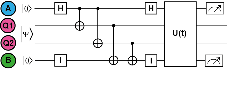
We consider the X𝑋X and Z𝑍Z stabilizer circuit as presented in appendix B of Fowler , however extended with unitary (Hamiltonian) evolution U​(t)π‘ˆπ‘‘U(t) for time duration t𝑑t, cf. Figure 1. The ideal quantum circuit does not include Uπ‘ˆU and is part of the in Fowler ; Brav ; Terhal outlined surface code. It is built with two data qubits and two ancillas, also called measure qubits. The corresponding measurement result is the error syndrome NC .
Refer to caption
Figure 1: Quantum X𝑋X and Z𝑍Z stabilizer circuit including unitary evolution; the ideal circuit does not include U​(t)π‘ˆπ‘‘U(t).

II.1 Circuit analysis

The ideal circuit is analyzed by Fowler in terms of the standard (computational) basis. For convenience, we repeat the analysis in terms of the Bell states in appendix B. In both ways it is demonstrated that the two data qubits are stabilized in a simultaneous eigenstate of X[1]​X[2]superscript𝑋delimited-[]1superscript𝑋delimited-[]2X^{[1]}X^{[2]} and Z[1]​Z[2]superscript𝑍delimited-[]1superscript𝑍delimited-[]2Z^{[1]}Z^{[2]}. These are exactly the Bell states:

X[1]​X[2]​|Ξ¦+⟩=|Ξ¦+⟩,superscript𝑋delimited-[]1superscript𝑋delimited-[]2ketsuperscriptΞ¦ketsuperscriptΞ¦\displaystyle X^{[1]}X^{[2]}|\Phi^{+}\rangle=|\Phi^{+}\rangle, X[1]​X[2]​|Ξ¨+⟩=|Ξ¨+⟩,superscript𝑋delimited-[]1superscript𝑋delimited-[]2ketsuperscriptΞ¨ketsuperscriptΞ¨\displaystyle X^{[1]}X^{[2]}|\Psi^{+}\rangle=|\Psi^{+}\rangle,
X[1]​X[2]​|Ξ¦βˆ’βŸ©=βˆ’|Ξ¦βˆ’βŸ©,superscript𝑋delimited-[]1superscript𝑋delimited-[]2ketsuperscriptΞ¦ketsuperscriptΞ¦\displaystyle X^{[1]}X^{[2]}|\Phi^{-}\rangle=-|\Phi^{-}\rangle, X[1]​X[2]​|Ξ¨βˆ’βŸ©=βˆ’|Ξ¨βˆ’βŸ©,superscript𝑋delimited-[]1superscript𝑋delimited-[]2ketsuperscriptΞ¨ketsuperscriptΞ¨\displaystyle X^{[1]}X^{[2]}|\Psi^{-}\rangle=-|\Psi^{-}\rangle,
Z[1]​Z[2]​|Ξ¦+⟩=|Ξ¦+⟩,superscript𝑍delimited-[]1superscript𝑍delimited-[]2ketsuperscriptΞ¦ketsuperscriptΞ¦\displaystyle Z^{[1]}Z^{[2]}|\Phi^{+}\rangle=|\Phi^{+}\rangle, Z[1]​Z[2]​|Ξ¨+⟩=βˆ’|Ξ¨+⟩,superscript𝑍delimited-[]1superscript𝑍delimited-[]2ketsuperscriptΞ¨ketsuperscriptΞ¨\displaystyle Z^{[1]}Z^{[2]}|\Psi^{+}\rangle=-|\Psi^{+}\rangle,
Z[1]​Z[2]​|Ξ¦βˆ’βŸ©=|Ξ¦βˆ’βŸ©,superscript𝑍delimited-[]1superscript𝑍delimited-[]2ketsuperscriptΞ¦ketsuperscriptΞ¦\displaystyle Z^{[1]}Z^{[2]}|\Phi^{-}\rangle=|\Phi^{-}\rangle, Z[1]​Z[2]​|Ξ¨βˆ’βŸ©=βˆ’|Ξ¨βˆ’βŸ©.superscript𝑍delimited-[]1superscript𝑍delimited-[]2ketsuperscriptΞ¨ketsuperscriptΞ¨\displaystyle Z^{[1]}Z^{[2]}|\Psi^{-}\rangle=-|\Psi^{-}\rangle. (1)

In other words, if we select one of these states as input to the circuit, it can readily be verified that the same output state state is obtained. The result of the ancilla measurement, the error syndrome, is reproduced as well with probability one. Thus we have shown that this indeed is a stabilizer circuit.

II.2 Error correction

Assume that we put a stable state into the circuit. As mentioned above, without errors, the ancilla measurement result is known. Suppose, however, that due to some error a different error syndrome is obtained. Concomitantly, the resulting two-qubit state has changed as well. Because the final state is nevertheless known, error correction by applying one or two single qubit operations is possible. We work out this procedure for two out of four cases, thereby explicitly constructing the necessary operations. Equations (A.127, A.128) are repeatedly used.

  • β€’

    State |Φ+⟩ketsuperscriptΦ|\Phi^{+}\rangle
    Error syndrome (+1,+1)11(+1,+1), that is no errors are detected; otherwise:

    • –

      Error syndrome (βˆ’1,+1)11(-1,+1), state |Ξ¦βˆ’βŸ©ketsuperscriptΞ¦|\Phi^{-}\rangle, correction Z[1]​|Ξ¦βˆ’βŸ©=|Ξ¦+⟩superscript𝑍delimited-[]1ketsuperscriptΞ¦ketsuperscriptΞ¦Z^{[1]}|\Phi^{-}\rangle=|\Phi^{+}\rangle.

    • –

      Error syndrome (+1,βˆ’1)11(+1,-1), state |Ξ¨+⟩ketsuperscriptΞ¨|\Psi^{+}\rangle, correction X[2]​|Ξ¨+⟩=|Ξ¦+⟩superscript𝑋delimited-[]2ketsuperscriptΞ¨ketsuperscriptΞ¦X^{[2]}|\Psi^{+}\rangle=|\Phi^{+}\rangle.

    • –

      Error syndrome (βˆ’1,βˆ’1)11(-1,-1), state |Ξ¨βˆ’βŸ©ketsuperscriptΞ¨|\Psi^{-}\rangle, correction X[2]​Z[1]​|Ξ¨βˆ’βŸ©=|Ξ¦+⟩superscript𝑋delimited-[]2superscript𝑍delimited-[]1ketsuperscriptΞ¨ketsuperscriptΞ¦X^{[2]}Z^{[1]}|\Psi^{-}\rangle=|\Phi^{+}\rangle.

  • β€’

    State |Ψ+⟩ketsuperscriptΨ|\Psi^{+}\rangle
    Error syndrome (+1,βˆ’1)11(+1,-1), that is no errors are detected; otherwise:

    • –

      Error syndrome (+1,+1)11(+1,+1), state |Ξ¦+⟩ketsuperscriptΞ¦|\Phi^{+}\rangle, correction X[1]​|Ξ¦+⟩=|Ξ¨+⟩superscript𝑋delimited-[]1ketsuperscriptΞ¦ketsuperscriptΞ¨X^{[1]}|\Phi^{+}\rangle=|\Psi^{+}\rangle.

    • –

      Error syndrome (βˆ’1,+1)11(-1,+1), state |Ξ¦βˆ’βŸ©ketsuperscriptΞ¦|\Phi^{-}\rangle, correction X[2]​Z[1]​|Ξ¦βˆ’βŸ©=|Ξ¨+⟩superscript𝑋delimited-[]2superscript𝑍delimited-[]1ketsuperscriptΞ¦ketsuperscriptΞ¨X^{[2]}Z^{[1]}|\Phi^{-}\rangle=|\Psi^{+}\rangle.

    • –

      Error syndrome (βˆ’1,βˆ’1)11(-1,-1), state |Ξ¨βˆ’βŸ©ketsuperscriptΞ¨|\Psi^{-}\rangle, correction Z[1]​|Ξ¨βˆ’βŸ©=|Ξ¨+⟩superscript𝑍delimited-[]1ketsuperscriptΞ¨ketsuperscriptΞ¨Z^{[1]}|\Psi^{-}\rangle=|\Psi^{+}\rangle.

Note that these error corrections are not unique, for example Z[2]​|Ξ¦βˆ’βŸ©=|Ξ¦+⟩superscript𝑍delimited-[]2ketsuperscriptΞ¦ketsuperscriptΞ¦Z^{[2]}|\Phi^{-}\rangle=|\Phi^{+}\rangle.

II.3 Dynamics

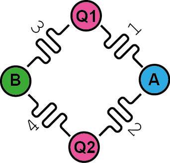
Two data qubits stabilized by one measure-X𝑋X qubit A𝐴A and one measure-Z𝑍Z qubit B𝐡B Fowler coupled by resonators are shown and labelled in Figure 2.
Refer to caption
Figure 2: Two data qubits and two ancillas coupled by four resonators.

The generalized Jaynes-Tavis-Cummings Hamiltonian for this system is given by Qudit

H𝐻\displaystyle H =\displaystyle= H0q+H0r+Hint11+Hint1​a+Hint2​a+Hint22superscriptsubscript𝐻0π‘žsuperscriptsubscript𝐻0π‘Ÿsuperscriptsubscript𝐻int11superscriptsubscript𝐻int1π‘Žsuperscriptsubscript𝐻int2π‘Žsuperscriptsubscript𝐻int22\displaystyle H_{0}^{q}+H_{0}^{r}+H_{\text{int}}^{11}+H_{\text{int}}^{1a}+H_{\text{int}}^{2a}+H_{\text{int}}^{22} (2)
+\displaystyle+ Hint31+Hint3​b+Hint4​b+Hint42,superscriptsubscript𝐻int31superscriptsubscript𝐻int3𝑏superscriptsubscript𝐻int4𝑏superscriptsubscript𝐻int42\displaystyle H_{\text{int}}^{31}+H_{\text{int}}^{3b}+H_{\text{int}}^{4b}+H_{\text{int}}^{42},

with the β€˜free’ qubit Hamiltonian

H0q=βˆ’12​ω1′​σz[1]βˆ’12​ωa​σz[a]βˆ’12​ω2′​σz[2]βˆ’12​ωb​σz[b]superscriptsubscript𝐻0π‘ž12superscriptsubscriptπœ”1β€²superscriptsubscriptπœŽπ‘§delimited-[]112subscriptπœ”π‘ŽsuperscriptsubscriptπœŽπ‘§delimited-[]π‘Ž12superscriptsubscriptπœ”2β€²superscriptsubscriptπœŽπ‘§delimited-[]212subscriptπœ”π‘superscriptsubscriptπœŽπ‘§delimited-[]𝑏H_{0}^{q}=-\tfrac{1}{2}\omega_{1}^{\prime}\sigma_{z}^{[1]}-\tfrac{1}{2}\omega_{a}\sigma_{z}^{[a]}-\tfrac{1}{2}\omega_{2}^{\prime}\sigma_{z}^{[2]}-\tfrac{1}{2}\omega_{b}\sigma_{z}^{[b]} (3)

and the Hamiltonian of the resonators

H0rsuperscriptsubscript𝐻0π‘Ÿ\displaystyle H_{0}^{r} =\displaystyle= Ο‰1​(a1†​a1+12)+Ο‰2​(a2†​a2+12)subscriptπœ”1superscriptsubscriptπ‘Ž1†subscriptπ‘Ž112subscriptπœ”2superscriptsubscriptπ‘Ž2†subscriptπ‘Ž212\displaystyle\omega_{1}(a_{1}^{\dagger}a_{1}+\tfrac{1}{2})+\omega_{2}(a_{2}^{\dagger}a_{2}+\tfrac{1}{2}) (4)
+\displaystyle+ Ο‰3​(a3†​a3+12)+Ο‰4​(a4†​a4+12).subscriptπœ”3superscriptsubscriptπ‘Ž3†subscriptπ‘Ž312subscriptπœ”4superscriptsubscriptπ‘Ž4†subscriptπ‘Ž412\displaystyle\omega_{3}(a_{3}^{\dagger}a_{3}+\tfrac{1}{2})+\omega_{4}(a_{4}^{\dagger}a_{4}+\tfrac{1}{2}).

The interaction terms in the rotating wave approximation read

Hint11superscriptsubscript𝐻int11\displaystyle H_{\text{int}}^{11} =\displaystyle= g11​(a1†​σ+[1]+a1β€‹Οƒβˆ’[1]),subscript𝑔11superscriptsubscriptπ‘Ž1†superscriptsubscript𝜎delimited-[]1subscriptπ‘Ž1superscriptsubscript𝜎delimited-[]1\displaystyle g_{11}\left(a_{1}^{\dagger}\sigma_{+}^{[1]}+a_{1}\sigma_{-}^{[1]}\right),
Hint1​asuperscriptsubscript𝐻int1π‘Ž\displaystyle H_{\text{int}}^{1a} =\displaystyle= g1​a​(a1†​σ+[a]+a1β€‹Οƒβˆ’[a]),etc.subscript𝑔1π‘Žsuperscriptsubscriptπ‘Ž1†superscriptsubscript𝜎delimited-[]π‘Žsubscriptπ‘Ž1superscriptsubscript𝜎delimited-[]π‘Žetc\displaystyle g_{1a}\left(a_{1}^{\dagger}\sigma_{+}^{[a]}+a_{1}\sigma_{-}^{[a]}\right),\quad\text{etc}. (5)

The frequencies are denoted by Ο‰k,k=1,…,4,formulae-sequencesubscriptπœ”π‘˜π‘˜1…4\omega_{k},k=1,\dots,4, for the resonators, Ο‰1β€²,Ο‰2β€²subscriptsuperscriptπœ”β€²1subscriptsuperscriptπœ”β€²2\omega^{\prime}_{1},\omega^{\prime}_{2} for the data qubits and Ο‰a,Ο‰bsubscriptπœ”π‘Žsubscriptπœ”π‘\omega_{a},\omega_{b} for the ancillas. The coupling constants are taken as g11,g1​a,g2​a,g22,g42,g4​b,g3​b,g31subscript𝑔11subscript𝑔1π‘Žsubscript𝑔2π‘Žsubscript𝑔22subscript𝑔42subscript𝑔4𝑏subscript𝑔3𝑏subscript𝑔31g_{11},g_{1a},g_{2a},g_{22},g_{42},g_{4b},g_{3b},g_{31}.

To study the dynamics, it is necessary to solve the SchrΓΆdinger equation, that is obtaining eigenenergies and eigenstates of the Hamiltonian. Herewith the evolution operator U​(t)π‘ˆπ‘‘U(t) is constructed. The technique of Qudit is applied, where excitation number operators for Jaynes-Tavis-Cummings Hamiltonians are exploited. For the system under consideration this operator 𝒩𝒩\mathcal{N} is given by

𝒩=βˆ‘k=14ak†​akβˆ’12​(Οƒz[1]+Οƒz[2]+Οƒz[a]+Οƒz[b]).𝒩superscriptsubscriptπ‘˜14superscriptsubscriptπ‘Žπ‘˜β€ subscriptπ‘Žπ‘˜12superscriptsubscriptπœŽπ‘§delimited-[]1superscriptsubscriptπœŽπ‘§delimited-[]2superscriptsubscriptπœŽπ‘§delimited-[]π‘ŽsuperscriptsubscriptπœŽπ‘§delimited-[]𝑏\mathcal{N}=\sum_{k=1}^{4}a_{k}^{\dagger}a_{k}-\tfrac{1}{2}(\sigma_{z}^{[1]}+\sigma_{z}^{[2]}+\sigma_{z}^{[a]}+\sigma_{z}^{[b]}). (6)

It commutes with the Hamiltonian: [𝒩,H]=0𝒩𝐻0[\mathcal{N},H]=0. Consequently, it is conserved and 𝒩𝒩\mathcal{N} and H𝐻H can be diagonalized simultaneously. Thus the dynamics can be analyzed separately for each excitation level.

The eigenstates of the excitation number operator are product states |r1,r2,r3,r4βŸ©βŠ—|q1,q2βŸ©βŠ—|qa,qb⟩tensor-productketsubscriptπ‘Ÿ1subscriptπ‘Ÿ2subscriptπ‘Ÿ3subscriptπ‘Ÿ4ketsubscriptπ‘ž1subscriptπ‘ž2ketsubscriptπ‘žπ‘Žsubscriptπ‘žπ‘|r_{1},r_{2},r_{3},r_{4}\rangle\otimes|q_{1},q_{2}\rangle\otimes|q_{a},q_{b}\rangle, with rk=0,1,2,…subscriptπ‘Ÿπ‘˜012…r_{k}=0,1,2,\dots for k=1,2,3,4π‘˜1234k=1,2,3,4 and qj=𝟎,𝟏subscriptπ‘žπ‘—01q_{j}=\bm{0,1} for j=1,2,a,b𝑗12π‘Žπ‘j=1,2,a,b. The lowest level 𝒩𝒩\mathcal{N} state is also the ground state of the Hamiltonian

|E0⟩=|0,0,0,0βŸ©βŠ—|𝟎,πŸŽβŸ©βŠ—|𝟎,𝟎⟩,ketsubscript𝐸0tensor-productket0000ket00ket00|E_{0}\rangle=|0,0,0,0\rangle\otimes|\bm{0},\bm{0}\rangle\otimes|\bm{0},\bm{0}\rangle, (7)

with energy eigenvalue

E0=12​(Ο‰1+Ο‰2+Ο‰3+Ο‰4βˆ’Ο‰1β€²βˆ’Ο‰2β€²βˆ’Ο‰aβˆ’Ο‰b).subscript𝐸012subscriptπœ”1subscriptπœ”2subscriptπœ”3subscriptπœ”4subscriptsuperscriptπœ”β€²1subscriptsuperscriptπœ”β€²2subscriptπœ”π‘Žsubscriptπœ”π‘E_{0}=\tfrac{1}{2}(\omega_{1}+\omega_{2}+\omega_{3}+\omega_{4}-\omega^{\prime}_{1}-\omega^{\prime}_{2}-\omega_{a}-\omega_{b}). (8)

The first excitation level is eight-fold degenerate with respect to 𝒩𝒩\mathcal{N}; we choose the basis states as given in appendix C. The matrix elements of the Hamiltonian in this subspace β„‹i​j,i,j=1,2,…​8formulae-sequencesubscriptℋ𝑖𝑗𝑖𝑗12…8\mathcal{H}_{ij},i,j=1,2,\dots 8 are also listed in appendix C. The corresponding eigenvalue problem needs to be solved:

ℋ​aΞΌ=E1​μ​aΞΌ,ΞΌ=1,2,…,8.formulae-sequenceβ„‹subscriptπ‘Žπœ‡subscript𝐸1πœ‡subscriptπ‘Žπœ‡πœ‡12…8\mathcal{H}a_{\mu}=E_{1\mu}a_{\mu},\quad\mu=1,2,\dots,8. (9)

As in Qudit , this is done by means of the Jacobi method. In this way, we obtain the eigenstates

|E1β€‹ΞΌβŸ©=βˆ‘k=18aμ​k​|ek⟩ketsubscript𝐸1πœ‡superscriptsubscriptπ‘˜18subscriptπ‘Žπœ‡π‘˜ketsubscriptπ‘’π‘˜|E_{1\mu}\rangle=\sum_{k=1}^{8}a_{\mu k}|e_{k}\rangle (10)

and the subspace evolution operator

U1​(t)=βˆ‘ΞΌ=18eβˆ’i​E1​μ​t​|E1β€‹ΞΌβŸ©β€‹βŸ¨E1​μ|.subscriptπ‘ˆ1𝑑superscriptsubscriptπœ‡18superscript𝑒𝑖subscript𝐸1πœ‡π‘‘ketsubscript𝐸1πœ‡brasubscript𝐸1πœ‡U_{1}(t)=\sum_{\mu=1}^{8}e^{-iE_{1\mu}t}|E_{1\mu}\rangle\langle E_{1\mu}|. (11)

We proceed to the second excitation level which has dimension thirty-two. See appendix C for our choice of basis states |fk⟩ketsubscriptπ‘“π‘˜|f_{k}\rangle. The matrix elements in the second excitation subspace 𝖧k​l,k,l=1,2,…,32formulae-sequencesubscriptπ–§π‘˜π‘™π‘˜π‘™12…32\mathsf{H}_{kl},k,l=1,2,\dots,32 are explicitly given in appendix C as well. The eigenvalue problem in this subspace

𝖧​bΞ·=E2​η​bΞ·,Ξ·=1,2,…,32,formulae-sequence𝖧subscriptπ‘πœ‚subscript𝐸2πœ‚subscriptπ‘πœ‚πœ‚12…32\mathsf{H}\,b_{\eta}=E_{2\eta}b_{\eta},\quad\eta=1,2,\dots,32, (12)

is again solved with the Jacobi method. It yields the eigenstates

|E2β€‹Ξ·βŸ©=βˆ‘l=132bη​l​|fl⟩ketsubscript𝐸2πœ‚superscriptsubscript𝑙132subscriptπ‘πœ‚π‘™ketsubscript𝑓𝑙|E_{2\eta}\rangle=\sum_{l=1}^{32}b_{\eta l}|f_{l}\rangle (13)

and the second excitation subspace evolution operator

U2​(t)=βˆ‘Ξ·=132eβˆ’i​E2​η​t​|E2β€‹Ξ·βŸ©β€‹βŸ¨E2​η|.subscriptπ‘ˆ2𝑑superscriptsubscriptπœ‚132superscript𝑒𝑖subscript𝐸2πœ‚π‘‘ketsubscript𝐸2πœ‚brasubscript𝐸2πœ‚U_{2}(t)=\sum_{\eta=1}^{32}e^{-iE_{2\eta}t}|E_{2\eta}\rangle\langle E_{2\eta}|. (14)

The constructed evolution operators will be used to compute specific unitary evolutions.

III Unitary evolution

In this paper, we presuppose that the X𝑋X and Z𝑍Z stabilizing circuit is ideal up to and including the last Hadamard operation, step 7. in appendix B. If one of the stable Bell states (A.126) has been put in, it is reproduced in (B.9) because the corresponding coefficient is one and the others are zero. Before completing the circuit by measuring the ancillas we now assume unitary evolution governed by the complete Hamiltonian and analyze the consequences. This is done for two initial states, containing the Bell states |Ξ¦+⟩ketsuperscriptΞ¦|\Phi^{+}\rangle and |Ξ¨+⟩ketsuperscriptΞ¨|\Psi^{+}\rangle. Assuming empty resonators, only the ground state and the second excitation subspace need to be taken into account. In principle, the analysis for the states |Ξ¦βˆ’βŸ©ketsuperscriptΞ¦|\Phi^{-}\rangle and |Ξ¨βˆ’βŸ©ketsuperscriptΞ¨|\Psi^{-}\rangle proceeds analogously. The corresponding states, however, have components in the third excitation subspace which makes computations more cumbersome. Therefore, we restrict ourselves to |Ξ¦+⟩ketsuperscriptΞ¦|\Phi^{+}\rangle and |Ξ¨+⟩ketsuperscriptΞ¨|\Psi^{+}\rangle.

III.1 Bell state |Φ+⟩ketsuperscriptΦ|\Phi^{+}\rangle

First, we assume that the two-qubit Bell state |Ξ¦+⟩ketsuperscriptΞ¦|\Phi^{+}\rangle has been put in the ideal stabilizer circuit. Then we study unitary evolution of the system after the last Hadamard operation has been performed. Thus the β€˜initial’ state follows from (B.9) with A+=1,B+=Aβˆ’=Bβˆ’=0formulae-sequencesubscript𝐴1subscript𝐡subscript𝐴subscript𝐡0A_{+}=1,B_{+}=A_{-}=B_{-}=0 and the inclusion with resonators, presumed to be empty

|Ο†0⟩=|0,0,0,0βŸ©βŠ—|Ξ¦+βŸ©βŠ—|𝟎,𝟎⟩.ketsubscriptπœ‘0tensor-productket0000ketsuperscriptΞ¦ket00|\varphi_{0}\rangle=|0,0,0,0\rangle\otimes|\Phi^{+}\rangle\otimes|\mathbf{0},\mathbf{0}\rangle. (15)

In terms of the defined basis vectors we get a superposition of the ground state and a state in the second excitation subspace

|Ο†0⟩=12​2​(|E0⟩+|f27⟩).ketsubscriptπœ‘0122ketsubscript𝐸0ketsubscript𝑓27|\varphi_{0}\rangle=\tfrac{1}{2}\sqrt{2}\left(|E_{0}\rangle+|f_{27}\rangle\right). (16)

Its unitary evolution is therefore given by

|φ​(t)⟩ketπœ‘π‘‘\displaystyle|\varphi(t)\rangle =\displaystyle= (U0​(t)+U1​(t)+U2​(t)+…)​|Ο†0⟩subscriptπ‘ˆ0𝑑subscriptπ‘ˆ1𝑑subscriptπ‘ˆ2𝑑…ketsubscriptπœ‘0\displaystyle\left(U_{0}(t)+U_{1}(t)+U_{2}(t)+\dots\right)|\varphi_{0}\rangle (17)
=\displaystyle= 12​2​(U​(t)​|E0⟩+U2​(t)​|f27⟩)122π‘ˆπ‘‘ketsubscript𝐸0subscriptπ‘ˆ2𝑑ketsubscript𝑓27\displaystyle\tfrac{1}{2}\sqrt{2}\left(U(t)|E_{0}\rangle+U_{2}(t)|f_{27}\rangle\right)
=\displaystyle= 12​2​(eβˆ’i​E0​t​|E0⟩+βˆ‘Ξ·=132eβˆ’i​E2​η​t​bη​27​|E2β€‹Ξ·βŸ©)122superscript𝑒𝑖subscript𝐸0𝑑ketsubscript𝐸0superscriptsubscriptπœ‚132superscript𝑒𝑖subscript𝐸2πœ‚π‘‘subscriptπ‘πœ‚27ketsubscript𝐸2πœ‚\displaystyle\tfrac{1}{2}\sqrt{2}\left(e^{-iE_{0}t}|E_{0}\rangle+\sum_{\eta=1}^{32}e^{-iE_{2\eta}t}b_{\eta 27}|E_{2\eta}\rangle\right)
=\displaystyle= 12​2​(eβˆ’i​E0​t​|E0⟩+βˆ‘Ξ·=132βˆ‘k=132eβˆ’i​E2​η​t​bη​27​bη​k​|fk⟩)122superscript𝑒𝑖subscript𝐸0𝑑ketsubscript𝐸0superscriptsubscriptπœ‚132superscriptsubscriptπ‘˜132superscript𝑒𝑖subscript𝐸2πœ‚π‘‘subscriptπ‘πœ‚27subscriptπ‘πœ‚π‘˜ketsubscriptπ‘“π‘˜\displaystyle\tfrac{1}{2}\sqrt{2}\left(e^{-iE_{0}t}|E_{0}\rangle+\sum_{\eta=1}^{32}\sum_{k=1}^{32}e^{-iE_{2\eta}t}b_{\eta 27}b_{\eta k}|f_{k}\rangle\right)
=\displaystyle= 12​2​eβˆ’i​E0​t​|E0⟩+βˆ‘k=132Ξ²k​(t)​|fk⟩,122superscript𝑒𝑖subscript𝐸0𝑑ketsubscript𝐸0superscriptsubscriptπ‘˜132subscriptπ›½π‘˜π‘‘ketsubscriptπ‘“π‘˜\displaystyle\tfrac{1}{2}\sqrt{2}e^{-iE_{0}t}|E_{0}\rangle+\sum_{k=1}^{32}\beta_{k}(t)|f_{k}\rangle,

where we have defined

Ξ²k​(t)=12​2β€‹βˆ‘Ξ·=132eβˆ’i​E2​η​t​bη​27​bη​k.subscriptπ›½π‘˜π‘‘122superscriptsubscriptπœ‚132superscript𝑒𝑖subscript𝐸2πœ‚π‘‘subscriptπ‘πœ‚27subscriptπ‘πœ‚π‘˜\beta_{k}(t)=\tfrac{1}{2}\sqrt{2}\sum_{\eta=1}^{32}e^{-iE_{2\eta}t}b_{\eta 27}b_{\eta k}. (18)

At this point we fix the time t𝑑t and perform the measurement on the ancillas. The measurement operator corresponding to the error syndrome (+1,+1)11(+1,+1) reads

P1,1=ℐr1βŠ—β„r2βŠ—β„r3βŠ—β„r4βŠ—β„12βŠ—| 0βŸ©β€‹βŸ¨πŸŽ|βŠ—| 0βŸ©β€‹βŸ¨πŸŽ|,subscript𝑃11tensor-producttensor-productsubscriptℐsubscriptπ‘Ÿ1subscriptℐsubscriptπ‘Ÿ2subscriptℐsubscriptπ‘Ÿ3subscriptℐsubscriptπ‘Ÿ4subscriptℐ12ket 0bra0ket 0bra0P_{1,1}=\mathcal{I}_{r_{1}}\otimes\mathcal{I}_{r_{2}}\otimes\mathcal{I}_{r_{3}}\otimes\mathcal{I}_{r_{4}}\otimes\mathcal{I}_{12}\otimes|\,\mathbf{0}\rangle\langle\mathbf{0}\,|\otimes|\,\mathbf{0}\rangle\langle\mathbf{0}\,|, (19)

with identity operators ℐrj,ℐ12=ℐ[1]βŠ—β„[2]subscriptℐsubscriptπ‘Ÿπ‘—subscriptℐ12tensor-productsuperscriptℐdelimited-[]1superscriptℐdelimited-[]2\mathcal{I}_{r_{j}},\mathcal{I}_{12}=\mathcal{I}^{[1]}\otimes\mathcal{I}^{[2]}. The probability that this result is obtained follows as

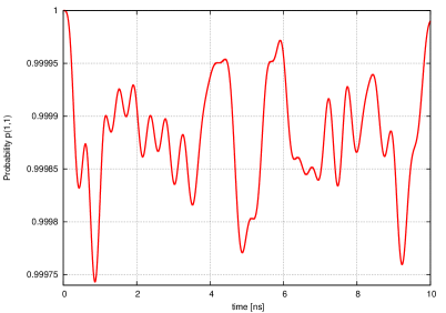
p​(1,1)=12+βˆ‘k∈S​(1,1)Ξ²kβˆ—β€‹(t)​βk​(t),𝑝1112subscriptπ‘˜π‘†11superscriptsubscriptπ›½π‘˜π‘‘subscriptπ›½π‘˜π‘‘p(1,1)=\tfrac{1}{2}+\sum_{k\in S(1,1)}\beta_{k}^{*}(t)\beta_{k}(t), (20)

where the integer set is given as

S​(1,1)={1,2,β‹―,12,15,16,19,20,23,24,27}.𝑆1112β‹―1215161920232427S(1,1)=\{1,2,\cdots,12,15,16,19,20,23,24,27\}. (21)

This result is depicted in Figure (3).
Refer to caption
Figure 3: Probability for obtaining the error syndrome (1,1) after unitary evolution of the state |0,0,0,0βŸ©β€‹|Ξ¦+βŸ©β€‹|𝟎,𝟎⟩ket0000ketsuperscriptΞ¦ket00|0,0,0,0\rangle|\Phi^{+}\rangle|\mathbf{0},\mathbf{0}\rangle as a function of time. Parameters: f1=8.14,f2=8.18,f3=8.1,f4=8.06,f1β€²=6.6,f2β€²=6.4,fa=5.9,fb=5.7formulae-sequencesubscript𝑓18.14formulae-sequencesubscript𝑓28.18formulae-sequencesubscript𝑓38.1formulae-sequencesubscript𝑓48.06formulae-sequencesuperscriptsubscript𝑓1β€²6.6formulae-sequencesuperscriptsubscript𝑓2β€²6.4formulae-sequencesubscriptπ‘“π‘Ž5.9subscript𝑓𝑏5.7f_{1}=8.14,f_{2}=8.18,f_{3}=8.1,f_{4}=8.06,f_{1}^{\prime}=6.6,f_{2}^{\prime}=6.4,f_{a}=5.9,f_{b}=5.7, g11=0.51,g22=0.52,g1​a=0.53,g2​a=0.54,g42=0.5,g4​b=0.49,g3​b=0.48,g31=0.47formulae-sequencesubscript𝑔110.51formulae-sequencesubscript𝑔220.52formulae-sequencesubscript𝑔1π‘Ž0.53formulae-sequencesubscript𝑔2π‘Ž0.54formulae-sequencesubscript𝑔420.5formulae-sequencesubscript𝑔4𝑏0.49formulae-sequencesubscript𝑔3𝑏0.48subscript𝑔310.47g_{11}=0.51,g_{22}=0.52,g_{1a}=0.53,g_{2a}=0.54,g_{42}=0.5,g_{4b}=0.49,g_{3b}=0.48,g_{31}=0.47; all values are given in GHz.

The state after projection and normalization follows as

|Ο†1,1⟩=1p​(1,1)​(12​2​eβˆ’i​E0​t​|E0⟩+βˆ‘k∈S​(1,1)Ξ²k​(t)​|fk⟩).ketsubscriptπœ‘111𝑝11122superscript𝑒𝑖subscript𝐸0𝑑ketsubscript𝐸0subscriptπ‘˜π‘†11subscriptπ›½π‘˜π‘‘ketsubscriptπ‘“π‘˜|\varphi_{1,1}\rangle=\frac{1}{\sqrt{p(1,1)}}\left(\tfrac{1}{2}\sqrt{2}e^{-iE_{0}t}|E_{0}\rangle+\sum_{k\in S(1,1)}\beta_{k}(t)|f_{k}\rangle\right). (22)

It can be written as a tensor product by factoring out the ancilla states

|Ο†1,1⟩=|Ο†~1,1βŸ©βŠ—| 0βŸ©βŠ—| 0⟩.ketsubscriptπœ‘11tensor-productketsubscript~πœ‘11ket 0ket 0|\varphi_{1,1}\rangle=|\tilde{\varphi}_{1,1}\rangle\otimes|\,\mathbf{0}\rangle\otimes|\,\mathbf{0}\rangle. (23)

The data qubits–resonators state, however, is still entangled.

We continue with measurements which indicate an error in the state. If the error syndrome equals (βˆ’1,1)11(-1,1), the corresponding measurement operator is given by

Pβˆ’1,1=ℐr1βŠ—β„r2βŠ—β„r3βŠ—β„r4βŠ—β„12βŠ—| 1βŸ©β€‹βŸ¨πŸ|βŠ—| 0βŸ©β€‹βŸ¨πŸŽ|.subscript𝑃11tensor-producttensor-productsubscriptℐsubscriptπ‘Ÿ1subscriptℐsubscriptπ‘Ÿ2subscriptℐsubscriptπ‘Ÿ3subscriptℐsubscriptπ‘Ÿ4subscriptℐ12ket1bra1ket 0bra0P_{-1,1}=\mathcal{I}_{r_{1}}\otimes\mathcal{I}_{r_{2}}\otimes\mathcal{I}_{r_{3}}\otimes\mathcal{I}_{r_{4}}\otimes\mathcal{I}_{12}\otimes|\,\mathbf{1}\rangle\langle\mathbf{1}\,|\otimes|\,\mathbf{0}\rangle\langle\mathbf{0}\,|. (24)

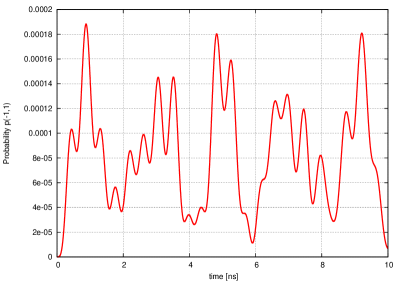
We obtain for the probability to find this result

p​(βˆ’1,1)=βˆ‘k∈S​(βˆ’1,1)Ξ²kβˆ—β€‹(t)​βk​(t),𝑝11subscriptπ‘˜π‘†11superscriptsubscriptπ›½π‘˜π‘‘subscriptπ›½π‘˜π‘‘p(-1,1)=\sum_{k\in S(-1,1)}\beta_{k}^{*}(t)\beta_{k}(t), (25)

with concomitant normalized state

|Ο†βˆ’1,1⟩=1p​(βˆ’1,1)β€‹βˆ‘k∈S​(βˆ’1,1)Ξ²k​(t)​|fk⟩ketsubscriptπœ‘111𝑝11subscriptπ‘˜π‘†11subscriptπ›½π‘˜π‘‘ketsubscriptπ‘“π‘˜|\varphi_{-1,1}\rangle=\frac{1}{\sqrt{p(-1,1)}}\sum_{k\in S(-1,1)}\beta_{k}(t)|f_{k}\rangle (26)

and the set

S​(βˆ’1,1)={13,17,21,25,28,30}.𝑆11131721252830S(-1,1)=\{13,17,21,25,28,30\}. (27)

The result for the probability is shown in Figure (4). The ancilla states can again be factored out

|Ο†βˆ’1,1⟩=|Ο†~βˆ’1,1βŸ©βŠ—| 1βŸ©βŠ—| 0⟩ketsubscriptπœ‘11tensor-productketsubscript~πœ‘11ket1ket 0|\varphi_{-1,1}\rangle=|\tilde{\varphi}_{-1,1}\rangle\otimes|\,\mathbf{1}\rangle\otimes|\,\mathbf{0}\rangle (28)

but data qubits and resonators remain entangled.
Refer to caption
Figure 4: Probability for obtaining the error syndrome (-1,1) after unitary evolution of the state |0,0,0,0βŸ©β€‹|Ξ¦+βŸ©β€‹|𝟎,𝟎⟩ket0000ketsuperscriptΞ¦ket00|0,0,0,0\rangle|\Phi^{+}\rangle|\mathbf{0},\mathbf{0}\rangle as a function of time. Parameters as in the previous figure.

The analogous results for obtaining the error syndrome (1,βˆ’1)11(1,-1) are

P1,βˆ’1=ℐr1βŠ—β„r2βŠ—β„r3βŠ—β„r4βŠ—β„12βŠ—| 0βŸ©β€‹βŸ¨πŸŽ|βŠ—| 1βŸ©β€‹βŸ¨πŸ|,subscript𝑃11tensor-producttensor-productsubscriptℐsubscriptπ‘Ÿ1subscriptℐsubscriptπ‘Ÿ2subscriptℐsubscriptπ‘Ÿ3subscriptℐsubscriptπ‘Ÿ4subscriptℐ12ket 0bra0ket1bra1P_{1,-1}=\mathcal{I}_{r_{1}}\otimes\mathcal{I}_{r_{2}}\otimes\mathcal{I}_{r_{3}}\otimes\mathcal{I}_{r_{4}}\otimes\mathcal{I}_{12}\otimes|\,\mathbf{0}\rangle\langle\mathbf{0}\,|\otimes|\,\mathbf{1}\rangle\langle\mathbf{1}\,|, (29)

with probability

p​(1,βˆ’1)=βˆ‘k∈S​(1,βˆ’1)Ξ²kβˆ—β€‹(t)​βk​(t),𝑝11subscriptπ‘˜π‘†11superscriptsubscriptπ›½π‘˜π‘‘subscriptπ›½π‘˜π‘‘p(1,-1)=\sum_{k\in S(1,-1)}\beta_{k}^{*}(t)\beta_{k}(t), (30)

state

|Ο†1,βˆ’1⟩=1p​(1,βˆ’1)β€‹βˆ‘k∈S​(1,βˆ’1)Ξ²k​(t)​|fk⟩,ketsubscriptπœ‘111𝑝11subscriptπ‘˜π‘†11subscriptπ›½π‘˜π‘‘ketsubscriptπ‘“π‘˜|\varphi_{1,-1}\rangle=\frac{1}{\sqrt{p(1,-1)}}\sum_{k\in S(1,-1)}\beta_{k}(t)|f_{k}\rangle, (31)

and integer set

S​(1,βˆ’1)={14,18,22,26,29,31}.𝑆11141822262931S(1,-1)=\{14,18,22,26,29,31\}. (32)

After amputating the ancillas, the state reads

|Ο†1,βˆ’1⟩=|Ο†~1,βˆ’1βŸ©βŠ—| 0βŸ©βŠ—| 1⟩.ketsubscriptπœ‘11tensor-productketsubscript~πœ‘11ket 0ket1|\varphi_{1,-1}\rangle=|\tilde{\varphi}_{1,-1}\rangle\otimes|\,\mathbf{0}\rangle\otimes|\,\mathbf{1}\rangle. (33)

Since p​(1,βˆ’1)<10βˆ’4𝑝11superscript104p(1,-1)<10^{-4}, it is not shown.

The error syndrome (βˆ’1,βˆ’1)11(-1,-1) corresponds to the operator

Pβˆ’1,βˆ’1=ℐr1βŠ—β„r2βŠ—β„r3βŠ—β„r4βŠ—β„12βŠ—| 1βŸ©β€‹βŸ¨πŸ|βŠ—| 1βŸ©β€‹βŸ¨πŸ|,subscript𝑃11tensor-producttensor-productsubscriptℐsubscriptπ‘Ÿ1subscriptℐsubscriptπ‘Ÿ2subscriptℐsubscriptπ‘Ÿ3subscriptℐsubscriptπ‘Ÿ4subscriptℐ12ket1bra1ket1bra1P_{-1,-1}=\mathcal{I}_{r_{1}}\otimes\mathcal{I}_{r_{2}}\otimes\mathcal{I}_{r_{3}}\otimes\mathcal{I}_{r_{4}}\otimes\mathcal{I}_{12}\otimes|\,\mathbf{1}\rangle\langle\mathbf{1}\,|\otimes|\,\mathbf{1}\rangle\langle\mathbf{1}\,|, (34)

which projects to one basis state

|Ο†βˆ’1,βˆ’1⟩=Ξ²32​(t)|Ξ²32​(t)|​|f32⟩,ketsubscriptπœ‘11subscript𝛽32𝑑subscript𝛽32𝑑ketsubscript𝑓32|\varphi_{-1,-1}\rangle=\frac{\beta_{32}(t)}{|\beta_{32}(t)|}|f_{32}\rangle, (35)

with probability

p​(βˆ’1,βˆ’1)=Ξ²32βˆ—β€‹(t)​β32​(t).𝑝11superscriptsubscript𝛽32𝑑subscript𝛽32𝑑p(-1,-1)=\beta_{32}^{*}(t)\beta_{32}(t). (36)

This probability is less than 10βˆ’7superscript10710^{-7}. The final state is a product state in all degrees of freedom

|Ο†βˆ’1,βˆ’1⟩=|0βŸ©βŠ—|0βŸ©βŠ—|0βŸ©βŠ—|0βŸ©βŠ—| 0βŸ©βŠ—| 0βŸ©βŠ—| 1βŸ©βŠ—| 1⟩,ketsubscriptπœ‘11tensor-productket0ket0ket0ket0ket 0ket 0ket1ket1|\varphi_{-1,-1}\rangle=|0\rangle\otimes|0\rangle\otimes|0\rangle\otimes|0\rangle\otimes|\,\mathbf{0}\rangle\otimes|\,\mathbf{0}\rangle\otimes|\,\mathbf{1}\rangle\otimes|\,\mathbf{1}\rangle, (37)

where we have omitted a phase factor.

III.2 Bell state |Ψ+⟩ketsuperscriptΨ|\Psi^{+}\rangle

We do a similar analysis for the Bell state |Ψ+⟩ketsuperscriptΨ|\Psi^{+}\rangle:

|ψ0⟩ketsubscriptπœ“0\displaystyle|\psi_{0}\rangle =\displaystyle= |0,0,0,0βŸ©βŠ—|Ξ¨+βŸ©βŠ—|𝟎,𝟏⟩tensor-productket0000ketsuperscriptΞ¨ket01\displaystyle|0,0,0,0\rangle\otimes|\Psi^{+}\rangle\otimes|\mathbf{0},\mathbf{1}\rangle (38)
=\displaystyle= 12​2​(|f29⟩+|f31⟩).122ketsubscript𝑓29ketsubscript𝑓31\displaystyle\tfrac{1}{2}\sqrt{2}\left(|f_{29}\rangle+|f_{31}\rangle\right).

Unitary evolution is governed by U2​(t)subscriptπ‘ˆ2𝑑U_{2}(t) and it yields

|Οˆβ€‹(t)⟩ketπœ“π‘‘\displaystyle|\psi(t)\rangle =\displaystyle= 12​2​U2​(t)​(|f29⟩+|f31⟩)122subscriptπ‘ˆ2𝑑ketsubscript𝑓29ketsubscript𝑓31\displaystyle\tfrac{1}{2}\sqrt{2}\,U_{2}(t)\left(|f_{29}\rangle+|f_{31}\rangle\right) (39)
=\displaystyle= 12​2β€‹βˆ‘Ξ·=132eβˆ’i​E2​η​t​(bη​29+bη​31)​|E2β€‹Ξ·βŸ©122superscriptsubscriptπœ‚132superscript𝑒𝑖subscript𝐸2πœ‚π‘‘subscriptπ‘πœ‚29subscriptπ‘πœ‚31ketsubscript𝐸2πœ‚\displaystyle\tfrac{1}{2}\sqrt{2}\sum_{\eta=1}^{32}e^{-iE_{2\eta}t}(b_{\eta 29}+b_{\eta 31})|E_{2\eta}\rangle
=\displaystyle= 12​2β€‹βˆ‘Ξ·=132βˆ‘k=132eβˆ’i​E2​η​t​(bη​29+bη​31)​bη​k​|fk⟩122superscriptsubscriptπœ‚132superscriptsubscriptπ‘˜132superscript𝑒𝑖subscript𝐸2πœ‚π‘‘subscriptπ‘πœ‚29subscriptπ‘πœ‚31subscriptπ‘πœ‚π‘˜ketsubscriptπ‘“π‘˜\displaystyle\tfrac{1}{2}\sqrt{2}\sum_{\eta=1}^{32}\sum_{k=1}^{32}e^{-iE_{2\eta}t}(b_{\eta 29}+b_{\eta 31})b_{\eta k}|f_{k}\rangle
=\displaystyle= βˆ‘k=132Ξ³k​(t)​|fk⟩,superscriptsubscriptπ‘˜132subscriptπ›Ύπ‘˜π‘‘ketsubscriptπ‘“π‘˜\displaystyle\sum_{k=1}^{32}\gamma_{k}(t)|f_{k}\rangle,

where we have abbreviated

Ξ³k​(t)=12​2β€‹βˆ‘Ξ·=132eβˆ’i​E2​η​t​(bη​29+bη​31)​bη​k.subscriptπ›Ύπ‘˜π‘‘122superscriptsubscriptπœ‚132superscript𝑒𝑖subscript𝐸2πœ‚π‘‘subscriptπ‘πœ‚29subscriptπ‘πœ‚31subscriptπ‘πœ‚π‘˜\gamma_{k}(t)=\tfrac{1}{2}\sqrt{2}\sum_{\eta=1}^{32}e^{-iE_{2\eta}t}(b_{\eta 29}+b_{\eta 31})b_{\eta k}. (40)

At this instant of time t𝑑t the measurement on the ancillas is done. The measurements operators are defined above. The error syndrome corresponding to no error detection reads (1,βˆ’1)11(1,-1). We obtain for the probability for obtaining these values

p​(1,βˆ’1)=βˆ‘k∈S​(1,βˆ’1)Ξ³kβˆ—β€‹(t)​γk​(t),𝑝11subscriptπ‘˜π‘†11superscriptsubscriptπ›Ύπ‘˜π‘‘subscriptπ›Ύπ‘˜π‘‘p(1,-1)=\sum_{k\in S(1,-1)}\gamma_{k}^{*}(t)\gamma_{k}(t), (41)

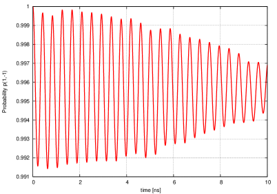
as shown in Figure (5).

Refer to caption
Figure 5: Probability for obtaining the error syndrome (1,-1) after unitary evolution of the state |0,0,0,0βŸ©β€‹|Ξ¨+βŸ©β€‹|𝟎,𝟏⟩ket0000ketsuperscriptΞ¨ket01|0,0,0,0\rangle|\Psi^{+}\rangle|\mathbf{0},\mathbf{1}\rangle as a function of time. Parameters as in Figure (3).

In order not to overload the notation we do not introduce a different symbol for probabilities in different examples. The corresponding normalized state is

|ψ1,βˆ’1⟩=1p​(1,βˆ’1)β€‹βˆ‘k∈S​(1,βˆ’1)Ξ³k​(t)​|fk⟩.ketsubscriptπœ“111𝑝11subscriptπ‘˜π‘†11subscriptπ›Ύπ‘˜π‘‘ketsubscriptπ‘“π‘˜|\psi_{1,-1}\rangle=\frac{1}{\sqrt{p(1,-1)}}\sum_{k\in S(1,-1)}\gamma_{k}(t)|f_{k}\rangle. (42)

The ancilla states can of course be separated

|ψ1,βˆ’1⟩=|ψ~1,βˆ’1βŸ©βŠ—| 0βŸ©βŠ—| 1⟩ketsubscriptπœ“11tensor-productketsubscript~πœ“11ket 0ket1|\psi_{1,-1}\rangle=|\tilde{\psi}_{1,-1}\rangle\otimes|\,\mathbf{0}\rangle\otimes|\,\mathbf{1}\rangle (43)

but once more the data qubits and resonators remain entangled.

The expressions for obtaining error syndromes indicating an error can be derived analogously and we merely present these without further comments:

p​(1,1)=βˆ‘k∈S​(1,1)Ξ³kβˆ—β€‹(t)​γk​(t),𝑝11subscriptπ‘˜π‘†11superscriptsubscriptπ›Ύπ‘˜π‘‘subscriptπ›Ύπ‘˜π‘‘p(1,1)=\sum_{k\in S(1,1)}\gamma_{k}^{*}(t)\gamma_{k}(t), (44)
|ψ1,1⟩ketsubscriptπœ“11\displaystyle|\psi_{1,1}\rangle =\displaystyle= 1p​(1,1)β€‹βˆ‘k∈S​(1,1)Ξ³k​(t)​|fk⟩1𝑝11subscriptπ‘˜π‘†11subscriptπ›Ύπ‘˜π‘‘ketsubscriptπ‘“π‘˜\displaystyle\frac{1}{\sqrt{p(1,1)}}\sum_{k\in S(1,1)}\gamma_{k}(t)|f_{k}\rangle (45)
=\displaystyle= |ψ~1,1βŸ©βŠ—| 0βŸ©βŠ—| 0⟩.tensor-productketsubscript~πœ“11ket 0ket 0\displaystyle|\tilde{\psi}_{1,1}\rangle\otimes|\,\mathbf{0}\rangle\otimes|\,\mathbf{0}\rangle.

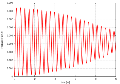
Figure (6) depicts the probability p​(1,1)𝑝11p(1,1).

Refer to caption
Figure 6: Probability for obtaining the error syndrome (1,1) after unitary evolution of the state |0,0,0,0βŸ©β€‹|Ξ¨+βŸ©β€‹|𝟎,𝟏⟩ket0000ketsuperscriptΞ¨ket01|0,0,0,0\rangle|\Psi^{+}\rangle|\mathbf{0},\mathbf{1}\rangle as a function of time. Parameters as in Figure (3).

For the error syndrome (βˆ’1,1)11(-1,1) we get

p​(βˆ’1,1)=βˆ‘k∈S​(βˆ’1,1)Ξ³kβˆ—β€‹(t)​γk​(t),𝑝11subscriptπ‘˜π‘†11superscriptsubscriptπ›Ύπ‘˜π‘‘subscriptπ›Ύπ‘˜π‘‘p(-1,1)=\sum_{k\in S(-1,1)}\gamma_{k}^{*}(t)\gamma_{k}(t), (46)
|Οˆβˆ’1,1⟩ketsubscriptπœ“11\displaystyle|\psi_{-1,1}\rangle =\displaystyle= 1p​(βˆ’1,1)β€‹βˆ‘k∈S​(βˆ’1,1)Ξ³k​(t)​|fk⟩1𝑝11subscriptπ‘˜π‘†11subscriptπ›Ύπ‘˜π‘‘ketsubscriptπ‘“π‘˜\displaystyle\frac{1}{\sqrt{p(-1,1)}}\sum_{k\in S(-1,1)}\gamma_{k}(t)|f_{k}\rangle (47)
=\displaystyle= |ψ~βˆ’1,1βŸ©βŠ—| 1βŸ©βŠ—| 0⟩.tensor-productketsubscript~πœ“11ket1ket 0\displaystyle|\tilde{\psi}_{-1,1}\rangle\otimes|\,\mathbf{1}\rangle\otimes|\,\mathbf{0}\rangle.

Because p​(βˆ’1,1)<10βˆ’5𝑝11superscript105p(-1,1)<10^{-5} it is not shown.

Finally, we obtain for the syndrome (βˆ’1,βˆ’1)11(-1,-1)

p​(βˆ’1,βˆ’1)=Ξ³32βˆ—β€‹(t)​γ32​(t),𝑝11superscriptsubscript𝛾32𝑑subscript𝛾32𝑑p(-1,-1)=\gamma_{32}^{*}(t)\gamma_{32}(t), (48)

which is less than 10βˆ’3superscript10310^{-3}. The final state

|Οˆβˆ’1,βˆ’1⟩=1p​(βˆ’1,βˆ’1)​γ32​(t)​|f32⟩ketsubscriptπœ“111𝑝11subscript𝛾32𝑑ketsubscript𝑓32|\psi_{-1,-1}\rangle=\frac{1}{\sqrt{p(-1,-1)}}\gamma_{32}(t)|f_{32}\rangle (49)

coincides -up to a phase factor- with (37).

IV Fidelities and error correction

In the last section, we have analyzed the four-qubit stabilizer system. Unitary evolution of the complete coupled system initially containing a separable stable Bell state has been calculated. There are two cases to be distinguished on the basis of the found error syndrome. In the first one, the syndrome indicates no error is and hence no error correction is applied. Secondly, the syndrome indicates a specific error which subsequently may be corrected by applying the correction operators on the data qubits, cf. section (II.2). In both cases, one then is interested in a measure how well the stabilizer performs. Note that in all cases the desired stable two-qubit state, or β€˜target state’, is known. Thus a natural choice would be the fidelity of the realized state. We have seen that in most cases, however, the two data qubits and the resonators are entangled and the concomitant two-qubit state is not defined. As a consequence, one needs to exploits the density matrix formalism Cohen1 ; NC and the technique of partial tracing. The latter reduces the density matrix of a composite system to the density matrix of a subsystem by performing the partial trace over the other degrees of freedom. The reduced density matrix of the data qubits is therefore obtained by tracing out the resonator degrees of freedom. Note, however, in case of entanglement the resulting subsystem density matrix will not correspond to a pure state. In our examples, the resonators-qubits state is of course pure and, with the exception of the product state after obtaing the error syndrome (βˆ’1,βˆ’1)11(-1,-1), entangled. Consequently, we cannot identify a pure two-qubit state since the density matrix corresponds to a mixed state. Nevertheless, we can use the concept of the fidelity between a pure (target) state |ψ⟩ketπœ“|\psi\rangle and the mixed state described by a density operator ρ𝜌\rho. It is defined as

F​(|ψ⟩,ρ)=⟨ψ|ρ|ψ⟩,𝐹ketπœ“πœŒquantum-operator-productπœ“πœŒπœ“F(|\psi\rangle,\rho)=\sqrt{\langle\psi|\rho|\psi\rangle}, (50)

cf. NC ; Carlo .

IV.1 Density matrix: Bell state |Φ+⟩ketsuperscriptΦ|\Phi^{+}\rangle

Once more we start the analysis for the case of the error syndrome (1,1)11(1,1). The state after having factored out the ancillas (23) is rewritten as

|Ο•~1,1⟩=1p​(1,1)β€‹βˆ‘k∈S~Ξ²k​(t)​|f~k⟩,ketsubscript~italic-Ο•111𝑝11subscriptπ‘˜~𝑆subscriptπ›½π‘˜π‘‘ketsubscript~π‘“π‘˜|\tilde{\phi}_{1,1}\rangle=\frac{1}{\sqrt{p(1,1)}}\sum_{k\in\tilde{S}}\beta_{k}(t)|\tilde{f}_{k}\rangle, (51)

thereby (implicitly) defining |f~k⟩ketsubscript~π‘“π‘˜|\tilde{f}_{k}\rangle, Ξ²0​(t)=12​2​eβˆ’i​E0​tsubscript𝛽0𝑑122superscript𝑒𝑖subscript𝐸0𝑑\beta_{0}(t)=\tfrac{1}{2}\sqrt{2}e^{-iE_{0}t} and S~={0}βˆͺS​(1,1)~𝑆0𝑆11\tilde{S}=\{0\}\cup S(1,1). The concomitant density matrix is therefore

ρ=1p​(1,1)β€‹βˆ‘k∈S~βˆ‘l∈S~Ξ²k​(t)​βlβˆ—β€‹(t)​|f~kβŸ©β€‹βŸ¨f~l|.𝜌1𝑝11subscriptπ‘˜~𝑆subscript𝑙~𝑆subscriptπ›½π‘˜π‘‘subscriptsuperscript𝛽𝑙𝑑ketsubscript~π‘“π‘˜brasubscript~𝑓𝑙\rho=\frac{1}{p(1,1)}\sum_{k\in\tilde{S}}\sum_{l\in\tilde{S}}\beta_{k}(t)\beta^{*}_{l}(t)|\tilde{f}_{k}\rangle\langle\tilde{f}_{l}|. (52)

At this point we take the partial trace with respect to the resonator degrees of freedom. The result for the reduced data qubit denstity operator is given by

ρqsubscriptπœŒπ‘ž\displaystyle\rho_{q} =\displaystyle= 1p​(1,1){βˆ‘k=010Ξ²kβˆ—(t)Ξ²k(t)|𝟎,𝟎⟩⟨𝟎,𝟎|+Ξ²27βˆ—(t)Ξ²27(t)|𝟏,𝟏⟩⟨𝟏,𝟏|\displaystyle\frac{1}{p(1,1)}\biggl{\{}\sum_{k=0}^{10}\beta^{*}_{k}(t)\beta_{k}(t)|\mathbf{0,0}\rangle\langle\mathbf{0,0}|+\beta^{*}_{27}(t)\beta_{27}(t)|\mathbf{1,1}\rangle\langle\mathbf{1,1}|
+\displaystyle+ βˆ‘k=11,15,19,23Ξ²kβˆ—β€‹(t)​βk​(t)​|𝟏,πŸŽβŸ©β€‹βŸ¨πŸ,𝟎|+βˆ‘k=12,16,20,24Ξ²kβˆ—β€‹(t)​βk​(t)|𝟎,πŸβŸ©β€‹βŸ¨πŸŽ,𝟏|subscriptπ‘˜11151923subscriptsuperscriptπ›½π‘˜π‘‘subscriptπ›½π‘˜π‘‘ket10quantum-operator-product10subscriptπ‘˜12162024subscriptsuperscriptπ›½π‘˜π‘‘subscriptπ›½π‘˜π‘‘01bra01\displaystyle\sum_{k=11,15,19,23}\beta^{*}_{k}(t)\beta_{k}(t)|\mathbf{1,0}\rangle\langle\mathbf{1,0}|+\sum_{k=12,16,20,24}\beta^{*}_{k}(t)\beta_{k}(t)|\mathbf{0,1}\rangle\langle\mathbf{0,1}|
+\displaystyle+ Ξ²0​(t)​β27βˆ—β€‹(t)​|𝟎,πŸŽβŸ©β€‹βŸ¨πŸ,𝟏|+Ξ²27​(t)​β0βˆ—β€‹(t)|𝟏,πŸβŸ©β€‹βŸ¨πŸŽ,𝟎|subscript𝛽0𝑑subscriptsuperscript𝛽27𝑑ket00quantum-operator-product11subscript𝛽27𝑑subscriptsuperscript𝛽0𝑑11bra00\displaystyle\beta_{0}(t)\beta^{*}_{27}(t)|\mathbf{0,0}\rangle\langle\mathbf{1,1}|+\beta_{27}(t)\beta^{*}_{0}(t)|\mathbf{1,1}\rangle\langle\mathbf{0,0}|
+\displaystyle+ (Ξ²11​(t)​β12βˆ—β€‹(t)+Ξ²15​(t)​β16βˆ—β€‹(t)+Ξ²19​(t)​β20βˆ—β€‹(t)+Ξ²23​(t)​β24βˆ—β€‹(t))​|𝟏,πŸŽβŸ©β€‹βŸ¨πŸŽ,𝟏|subscript𝛽11𝑑subscriptsuperscript𝛽12𝑑subscript𝛽15𝑑subscriptsuperscript𝛽16𝑑subscript𝛽19𝑑subscriptsuperscript𝛽20𝑑subscript𝛽23𝑑subscriptsuperscript𝛽24𝑑ket10bra01\displaystyle\left(\beta_{11}(t)\beta^{*}_{12}(t)+\beta_{15}(t)\beta^{*}_{16}(t)+\beta_{19}(t)\beta^{*}_{20}(t)+\beta_{23}(t)\beta^{*}_{24}(t)\right)|\mathbf{1,0}\rangle\langle\mathbf{0,1}|
+\displaystyle+ (Ξ²12(t)Ξ²11βˆ—(t)+Ξ²16(t)Ξ²15βˆ—(t)+Ξ²20(t)Ξ²19βˆ—(t)+Ξ²24(t)Ξ²23βˆ—(t))|𝟎,𝟏⟩⟨𝟏,𝟎|}.\displaystyle\left(\beta_{12}(t)\beta^{*}_{11}(t)+\beta_{16}(t)\beta^{*}_{15}(t)+\beta_{20}(t)\beta^{*}_{19}(t)+\beta_{24}(t)\beta^{*}_{23}(t)\right)|\mathbf{0,1}\rangle\langle\mathbf{1,0}|\biggr{\}}.

We eventually obtain the fidelity

F​(|Ξ¦+⟩,ρq)=⟨Φ+|ρq|Ξ¦+⟩𝐹ketsuperscriptΞ¦subscriptπœŒπ‘žquantum-operator-productsuperscriptΞ¦subscriptπœŒπ‘žsuperscriptΞ¦\displaystyle F(|\Phi^{+}\rangle,\rho_{q})=\sqrt{\langle\Phi^{+}|\rho_{q}|\Phi^{+}\rangle} =\displaystyle= {12​p​(1,1)​[βˆ‘k=010Ξ²kβˆ—β€‹(t)​βk​(t)+Ξ²27βˆ—β€‹(t)​β27​(t)+Ξ²0βˆ—β€‹(t)​β27​(t)+Ξ²27βˆ—β€‹(t)​β0​(t)]}1/2,superscript12𝑝11delimited-[]superscriptsubscriptπ‘˜010subscriptsuperscriptπ›½π‘˜π‘‘subscriptπ›½π‘˜π‘‘subscriptsuperscript𝛽27𝑑subscript𝛽27𝑑subscriptsuperscript𝛽0𝑑subscript𝛽27𝑑subscriptsuperscript𝛽27𝑑subscript𝛽0𝑑12\displaystyle\left\{\frac{1}{2p(1,1)}\biggl{[}\sum_{k=0}^{10}\beta^{*}_{k}(t)\beta_{k}(t)+\beta^{*}_{27}(t)\beta_{27}(t)+\beta^{*}_{0}(t)\beta_{27}(t)+\beta^{*}_{27}(t)\beta_{0}(t)\biggr{]}\right\}^{1/2},

which is shown in Figure (7).

Refer to caption
Figure 7: Fidelity as a function of time after unitary evolution of the state |0,0,0,0βŸ©β€‹|Ξ¦+βŸ©β€‹|𝟎,𝟎⟩ket0000ketsuperscriptΞ¦ket00|0,0,0,0\rangle|\Phi^{+}\rangle|\mathbf{0},\mathbf{0}\rangle and subsequently obtaining error syndrome (1,1)11(1,1). Parameters as in Figure (3).

After having detected an error, one may apply a correction operator to the state. We analyze the consequences by computing the fidelity of the obtained target state and the reduced density operator. Since the partial trace is taken with respect to the resonators degrees of freedom and the error correction only operates on the data qubits, we can first compute the reduced density matrix and eventually apply the error correction operator on the target state. We demonstrate the method for the various error syndromes indicating an error.

For the syndrome (βˆ’1,1)11(-1,1) the state after factoring out the ancillas reads

|Ο•~βˆ’1,1⟩=1p​(βˆ’1,1)β€‹βˆ‘k∈S​(βˆ’1,1)Ξ²k​(t)​|f~k⟩,ketsubscript~italic-Ο•111𝑝11subscriptπ‘˜π‘†11subscriptπ›½π‘˜π‘‘ketsubscript~π‘“π‘˜|\tilde{\phi}_{-1,1}\rangle=\frac{1}{\sqrt{p(-1,1)}}\sum_{k\in S(-1,1)}\beta_{k}(t)|\tilde{f}_{k}\rangle, (54)

with corresponding density matrix

ρ=1p​(βˆ’1,1)β€‹βˆ‘k∈S​(βˆ’1,1)βˆ‘l∈S​(βˆ’1,1)Ξ²k​(t)​βlβˆ—β€‹(t)​|f~kβŸ©β€‹βŸ¨f~l|.𝜌1𝑝11subscriptπ‘˜π‘†11subscript𝑙𝑆11subscriptπ›½π‘˜π‘‘subscriptsuperscript𝛽𝑙𝑑ketsubscript~π‘“π‘˜brasubscript~𝑓𝑙\rho=\frac{1}{p(-1,1)}\sum_{k\in S(-1,1)}\sum_{l\in S(-1,1)}\beta_{k}(t)\beta^{*}_{l}(t)|\tilde{f}_{k}\rangle\langle\tilde{f}_{l}|. (55)

The reduced qubit density matrix follows as

ρqsubscriptπœŒπ‘ž\displaystyle\rho_{q} =\displaystyle= 1p​(βˆ’1,1){βˆ‘k=13,17,21,25Ξ²kβˆ—(t)Ξ²k(t)|𝟎,𝟎⟩⟨𝟎,𝟎|\displaystyle\frac{1}{p(-1,1)}\biggl{\{}\sum_{k=13,17,21,25}\beta^{*}_{k}(t)\beta_{k}(t)|\mathbf{0,0}\rangle\langle\mathbf{0,0}|
+\displaystyle+ Ξ²28​(t)​β28βˆ—β€‹(t)​|𝟏,πŸŽβŸ©β€‹βŸ¨πŸ,𝟎|+Ξ²30​(t)​β30βˆ—β€‹(t)|𝟎,πŸβŸ©β€‹βŸ¨πŸŽ,𝟏|subscript𝛽28𝑑subscriptsuperscript𝛽28𝑑ket10quantum-operator-product10subscript𝛽30𝑑subscriptsuperscript𝛽30𝑑01bra01\displaystyle\beta_{28}(t)\beta^{*}_{28}(t)|\mathbf{1,0}\rangle\langle\mathbf{1,0}|+\beta_{30}(t)\beta^{*}_{30}(t)|\mathbf{0,1}\rangle\langle\mathbf{0,1}|
+\displaystyle+ Ξ²28(t)Ξ²30βˆ—(t)|𝟏,𝟎⟩⟨𝟎,𝟏|+Ξ²30(t)Ξ²28βˆ—(t)|𝟎,𝟏⟩⟨𝟏,𝟎|}.\displaystyle\beta_{28}(t)\beta^{*}_{30}(t)|\mathbf{1,0}\rangle\langle\mathbf{0,1}|+\beta_{30}(t)\beta^{*}_{28}(t)|\mathbf{0,1}\rangle\langle\mathbf{1,0}|\biggr{\}}.

Herewith we get as fidelity

F​(|Ξ¦+⟩,Z[1]​ρq​Z[1])=⟨Φ+|Z[1]​ρq​Z[1]|Ξ¦+⟩=βŸ¨Ξ¦βˆ’|ρq|Ξ¦βˆ’βŸ©πΉketsuperscriptΞ¦superscript𝑍delimited-[]1subscriptπœŒπ‘žsuperscript𝑍delimited-[]1quantum-operator-productsuperscriptΞ¦superscript𝑍delimited-[]1subscriptπœŒπ‘žsuperscript𝑍delimited-[]1superscriptΞ¦quantum-operator-productsuperscriptΞ¦subscriptπœŒπ‘žsuperscriptΞ¦\displaystyle F(|\Phi^{+}\rangle,Z^{[1]}\rho_{q}Z^{[1]})=\sqrt{\langle\Phi^{+}|Z^{[1]}\rho_{q}Z^{[1]}|\Phi^{+}\rangle}=\sqrt{\langle\Phi^{-}|\rho_{q}|\Phi^{-}\rangle} (57)
=\displaystyle= {12​p​(βˆ’1,1)​[Ξ²13βˆ—β€‹(t)​β13​(t)+Ξ²17βˆ—β€‹(t)​β17​(t)+Ξ²21βˆ—β€‹(t)​β21​(t)+Ξ²25βˆ—β€‹(t)​β25​(t)]}1/2,superscript12𝑝11delimited-[]subscriptsuperscript𝛽13𝑑subscript𝛽13𝑑subscriptsuperscript𝛽17𝑑subscript𝛽17𝑑subscriptsuperscript𝛽21𝑑subscript𝛽21𝑑subscriptsuperscript𝛽25𝑑subscript𝛽25𝑑12\displaystyle\left\{\frac{1}{2p(-1,1)}\biggl{[}\beta^{*}_{13}(t)\beta_{13}(t)+\beta^{*}_{17}(t)\beta_{17}(t)+\beta^{*}_{21}(t)\beta_{21}(t)+\beta^{*}_{25}(t)\beta_{25}(t)\biggr{]}\right\}^{1/2},

which is close to zero.

Analogously, for the error syndrome (1,βˆ’1)11(1,-1) the state after factoring out the ancillas is given by

|Ο•~1,βˆ’1⟩=1p​(1,βˆ’1)β€‹βˆ‘k∈S​(1,βˆ’1)Ξ²k​(t)​|f~k⟩,ketsubscript~italic-Ο•111𝑝11subscriptπ‘˜π‘†11subscriptπ›½π‘˜π‘‘ketsubscript~π‘“π‘˜|\tilde{\phi}_{1,-1}\rangle=\frac{1}{\sqrt{p(1,-1)}}\sum_{k\in S(1,-1)}\beta_{k}(t)|\tilde{f}_{k}\rangle, (58)

with concomitant density matrix

ρ=1p​(1,βˆ’1)β€‹βˆ‘k∈S​(1,βˆ’1)βˆ‘l∈S​(1,βˆ’1)Ξ²k​(t)​βlβˆ—β€‹(t)​|f~kβŸ©β€‹βŸ¨f~l|.𝜌1𝑝11subscriptπ‘˜π‘†11subscript𝑙𝑆11subscriptπ›½π‘˜π‘‘subscriptsuperscript𝛽𝑙𝑑ketsubscript~π‘“π‘˜brasubscript~𝑓𝑙\rho=\frac{1}{p(1,-1)}\sum_{k\in S(1,-1)}\sum_{l\in S(1,-1)}\beta_{k}(t)\beta^{*}_{l}(t)|\tilde{f}_{k}\rangle\langle\tilde{f}_{l}|. (59)

Calculating the partial trace yields

ρqsubscriptπœŒπ‘ž\displaystyle\rho_{q} =\displaystyle= 1p​(1,βˆ’1){βˆ‘k=14,18,22,26Ξ²kβˆ—(t)Ξ²k(t)|𝟎,𝟎⟩⟨𝟎,𝟎|+Ξ²29(t)Ξ²29βˆ—(t)|𝟏,𝟎⟩⟨𝟏,𝟎|+Ξ²31(t)Ξ²31βˆ—(t)|𝟎,𝟏⟩⟨𝟎,𝟏|\displaystyle\frac{1}{p(1,-1)}\biggl{\{}\sum_{k=14,18,22,26}\beta^{*}_{k}(t)\beta_{k}(t)|\mathbf{0,0}\rangle\langle\mathbf{0,0}|+\beta_{29}(t)\beta^{*}_{29}(t)|\mathbf{1,0}\rangle\langle\mathbf{1,0}|+\beta_{31}(t)\beta^{*}_{31}(t)|\mathbf{0,1}\rangle\langle\mathbf{0,1}| (60)
+\displaystyle+ Ξ²29(t)Ξ²31βˆ—(t)|𝟏,𝟎⟩⟨𝟎,𝟏|+Ξ²31(t)Ξ²29βˆ—(t)|𝟎,𝟏⟩⟨𝟏,𝟎|}.\displaystyle\beta_{29}(t)\beta^{*}_{31}(t)|\mathbf{1,0}\rangle\langle\mathbf{0,1}|+\beta_{31}(t)\beta^{*}_{29}(t)|\mathbf{0,1}\rangle\langle\mathbf{1,0}|\biggr{\}}.

Subsequently, we obtain the fidelity

F​(|Ξ¦+⟩,X[2]​ρq​X[2])=⟨Φ+|X[2]​ρq​X[2]|Ξ¦+⟩=⟨Ψ+|ρq|Ξ¨+⟩𝐹ketsuperscriptΞ¦superscript𝑋delimited-[]2subscriptπœŒπ‘žsuperscript𝑋delimited-[]2quantum-operator-productsuperscriptΞ¦superscript𝑋delimited-[]2subscriptπœŒπ‘žsuperscript𝑋delimited-[]2superscriptΞ¦quantum-operator-productsuperscriptΞ¨subscriptπœŒπ‘žsuperscriptΞ¨\displaystyle F(|\Phi^{+}\rangle,X^{[2]}\rho_{q}X^{[2]})=\sqrt{\langle\Phi^{+}|X^{[2]}\rho_{q}X^{[2]}|\Phi^{+}\rangle}=\sqrt{\langle\Psi^{+}|\rho_{q}|\Psi^{+}\rangle} (61)
=\displaystyle= {12​p​(1,βˆ’1)​[Ξ²29βˆ—β€‹(t)​β29​(t)+Ξ²31βˆ—β€‹(t)​β31​(t)+Ξ²31βˆ—β€‹(t)​β29​(t)+Ξ²29βˆ—β€‹(t)​β31​(t)]}1/2,superscript12𝑝11delimited-[]subscriptsuperscript𝛽29𝑑subscript𝛽29𝑑subscriptsuperscript𝛽31𝑑subscript𝛽31𝑑subscriptsuperscript𝛽31𝑑subscript𝛽29𝑑subscriptsuperscript𝛽29𝑑subscript𝛽31𝑑12\displaystyle\left\{\frac{1}{2p(1,-1)}\biggl{[}\beta^{*}_{29}(t)\beta_{29}(t)+\beta^{*}_{31}(t)\beta_{31}(t)+\beta^{*}_{31}(t)\beta_{29}(t)+\beta^{*}_{29}(t)\beta_{31}(t)\biggr{]}\right\}^{1/2},

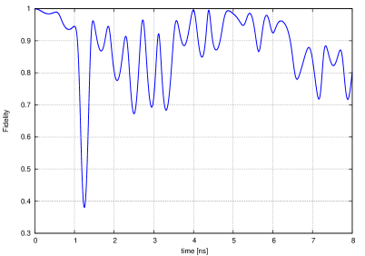
as shown in Figure (8).

Refer to caption
Figure 8: Fidelity as a function of time after unitary evolution of the state |0,0,0,0βŸ©β€‹|Ξ¦+βŸ©β€‹|𝟎,𝟎⟩ket0000ketsuperscriptΞ¦ket00|0,0,0,0\rangle|\Phi^{+}\rangle|\mathbf{0},\mathbf{0}\rangle, subsequently obtaining error syndrome (1,βˆ’1)11(1,-1) and error correction. Parameters as in Figure (3).

In case of error syndrome (βˆ’1,βˆ’1)11(-1,-1), it is easily seen that the reduced density matrix corresponds to a the pure state

ρq=|𝟎,πŸŽβŸ©β€‹βŸ¨πŸŽ,𝟎|.subscriptπœŒπ‘žket00bra00\rho_{q}=|\mathbf{0,0}\rangle\langle\mathbf{0,0}|. (62)

Then we get

F​(|Ξ¦+⟩,X[2]​Z[1]​ρq​Z[1]​X[2])𝐹ketsuperscriptΞ¦superscript𝑋delimited-[]2superscript𝑍delimited-[]1subscriptπœŒπ‘žsuperscript𝑍delimited-[]1superscript𝑋delimited-[]2\displaystyle F(|\Phi^{+}\rangle,X^{[2]}Z^{[1]}\rho_{q}Z^{[1]}X^{[2]}) (63)
=\displaystyle= ⟨Φ+|Z[1]​X[2]​ρq​Z[1]​X[2]|Ξ¦+⟩quantum-operator-productsuperscriptΞ¦superscript𝑍delimited-[]1superscript𝑋delimited-[]2subscriptπœŒπ‘žsuperscript𝑍delimited-[]1superscript𝑋delimited-[]2superscriptΞ¦\displaystyle\sqrt{\langle\Phi^{+}|Z^{[1]}X^{[2]}\rho_{q}Z^{[1]}X^{[2]}|\Phi^{+}\rangle}
=\displaystyle= βŸ¨Ξ¨βˆ’|ρq|Ξ¨βˆ’βŸ©=0,quantum-operator-productsuperscriptΞ¨subscriptπœŒπ‘žsuperscriptΞ¨0\displaystyle\sqrt{\langle\Psi^{-}|\rho_{q}|\Psi^{-}\rangle}=0,

that is a vanishing fidelity.

IV.2 Density matrix: Bell state |Ψ+⟩ketsuperscriptΨ|\Psi^{+}\rangle

The computations for the Bell state |Ξ¨+⟩ketsuperscriptΞ¨|\Psi^{+}\rangle of course proceed completely analogously and we merely present the results for the obtained fidelities. For the error syndrome (1,βˆ’1)11(1,-1), we get

F​(|Ξ¨+⟩,ρq)=⟨Ψ+|ρq|Ξ¨+⟩={12​p​(1,βˆ’1)​[Ξ³29βˆ—β€‹(t)​γ29​(t)+Ξ³31βˆ—β€‹(t)​γ31​(t)+Ξ³31βˆ—β€‹(t)​γ29​(t)+Ξ³29βˆ—β€‹(t)​γ31​(t)]}1/2.𝐹ketsuperscriptΞ¨subscriptπœŒπ‘žquantum-operator-productsuperscriptΞ¨subscriptπœŒπ‘žsuperscriptΞ¨superscript12𝑝11delimited-[]subscriptsuperscript𝛾29𝑑subscript𝛾29𝑑subscriptsuperscript𝛾31𝑑subscript𝛾31𝑑subscriptsuperscript𝛾31𝑑subscript𝛾29𝑑subscriptsuperscript𝛾29𝑑subscript𝛾31𝑑12F(|\Psi^{+}\rangle,\rho_{q})=\sqrt{\langle\Psi^{+}|\rho_{q}|\Psi^{+}\rangle}=\left\{\frac{1}{2p(1,-1)}\biggl{[}\gamma^{*}_{29}(t)\gamma_{29}(t)+\gamma^{*}_{31}(t)\gamma_{31}(t)+\gamma^{*}_{31}(t)\gamma_{29}(t)+\gamma^{*}_{29}(t)\gamma_{31}(t)\biggr{]}\right\}^{1/2}. (64)

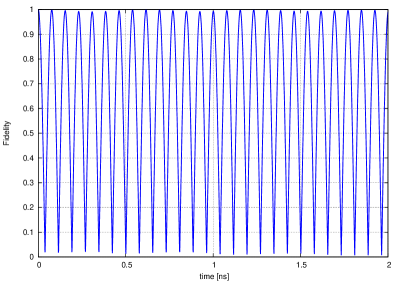
This fidelity is shown in Figure (9).

In case of obtaining the error syndrome (1,1)11(1,1), the resulting error corrected fidelity follows as

F​(|Ξ¨+⟩,X[1]​ρq​X[1])=⟨Ψ+|X[1]​ρq​X[1]|Ξ¨+⟩=⟨Φ+|ρq|Ξ¦+⟩={12​p​(1,1)​[βˆ‘k=110Ξ³kβˆ—β€‹(t)​γk​(t)+Ξ³27βˆ—β€‹(t)​γ27​(t)]}1/2,𝐹ketsuperscriptΞ¨superscript𝑋delimited-[]1subscriptπœŒπ‘žsuperscript𝑋delimited-[]1quantum-operator-productsuperscriptΞ¨superscript𝑋delimited-[]1subscriptπœŒπ‘žsuperscript𝑋delimited-[]1superscriptΞ¨quantum-operator-productsuperscriptΞ¦subscriptπœŒπ‘žsuperscriptΞ¦superscript12𝑝11delimited-[]superscriptsubscriptπ‘˜110subscriptsuperscriptπ›Ύπ‘˜π‘‘subscriptπ›Ύπ‘˜π‘‘subscriptsuperscript𝛾27𝑑subscript𝛾27𝑑12F(|\Psi^{+}\rangle,X^{[1]}\rho_{q}X^{[1]})=\sqrt{\langle\Psi^{+}|X^{[1]}\rho_{q}X^{[1]}|\Psi^{+}\rangle}=\sqrt{\langle\Phi^{+}|\rho_{q}|\Phi^{+}\rangle}=\left\{\frac{1}{2p(1,1)}\biggl{[}\sum_{k=1}^{10}\gamma^{*}_{k}(t)\gamma_{k}(t)+\gamma^{*}_{27}(t)\gamma_{27}(t)\biggr{]}\right\}^{1/2}, (65)

which is less than 0.0035 and therefore not shown here.

After error detection by means of the syndrome (βˆ’1,1)11(-1,1), we obtain as fidelity

F​(|Ξ¨+⟩,X[2]​Z[1]​ρq​Z[1]​X[2])=⟨Ψ+|X[2]​Z[1]​ρq​Z[1]​X[2]|Ξ¨+⟩=βŸ¨Ξ¦βˆ’|ρq|Ξ¦βˆ’βŸ©πΉketsuperscriptΞ¨superscript𝑋delimited-[]2superscript𝑍delimited-[]1subscriptπœŒπ‘žsuperscript𝑍delimited-[]1superscript𝑋delimited-[]2quantum-operator-productsuperscriptΞ¨superscript𝑋delimited-[]2superscript𝑍delimited-[]1subscriptπœŒπ‘žsuperscript𝑍delimited-[]1superscript𝑋delimited-[]2superscriptΞ¨quantum-operator-productsuperscriptΞ¦subscriptπœŒπ‘žsuperscriptΞ¦\displaystyle F(|\Psi^{+}\rangle,X^{[2]}Z^{[1]}\rho_{q}Z^{[1]}X^{[2]})=\sqrt{\langle\Psi^{+}|X^{[2]}Z^{[1]}\rho_{q}Z^{[1]}X^{[2]}|\Psi^{+}\rangle}=\sqrt{\langle\Phi^{-}|\rho_{q}|\Phi^{-}\rangle} (66)
=\displaystyle= {12​p​(βˆ’1,1)​[Ξ³13βˆ—β€‹(t)​γ13​(t)+Ξ³17βˆ—β€‹(t)​γ17​(t)+Ξ³21βˆ—β€‹(t)​γ21​(t)+Ξ³25βˆ—β€‹(t)​γ25​(t)]}1/2.superscript12𝑝11delimited-[]subscriptsuperscript𝛾13𝑑subscript𝛾13𝑑subscriptsuperscript𝛾17𝑑subscript𝛾17𝑑subscriptsuperscript𝛾21𝑑subscript𝛾21𝑑subscriptsuperscript𝛾25𝑑subscript𝛾25𝑑12\displaystyle\left\{\frac{1}{2p(-1,1)}\biggl{[}\gamma^{*}_{13}(t)\gamma_{13}(t)+\gamma^{*}_{17}(t)\gamma_{17}(t)+\gamma^{*}_{21}(t)\gamma_{21}(t)+\gamma^{*}_{25}(t)\gamma_{25}(t)\biggr{]}\right\}^{1/2}.

It turns out be aprroximately constant, very close to the value 12​2122\tfrac{1}{2}\sqrt{2}.

The case with error syndrome (βˆ’1,βˆ’1)11(-1,-1) once more yields a vanishing fidelity.
Refer to caption
Figure 9: Fidelity as a function of time after unitary evolution of the state |0,0,0,0βŸ©β€‹|Ξ¨+βŸ©β€‹|𝟎,𝟏⟩ket0000ketsuperscriptΞ¨ket01|0,0,0,0\rangle|\Psi^{+}\rangle|\mathbf{0},\mathbf{1}\rangle and subsequently obtaining error syndrome (1,βˆ’1)11(1,-1). Parameters as in Figure (3).

V Re-insertion into the circuit

The stabilizer circuit has the property that re-inserting the stable state into the circuit, reproduces it. The interesting question arises how this is possibly influenced by the unitary evolution governed by the Hamiltonian before the re-insertion. We analyze this problem once more for the two stable Bell states situations for which we have already calculated the evolution. Note that we assume a certain duration of the evolution before entering the circuit again. We emphasize that this duration is arbitrary but then fixed.

V.1 Bell state |Φ+⟩ketsuperscriptΦ|\Phi^{+}\rangle

In this case, we have to consider as initial state

|Ο†in⟩=1p​(1,1)β€‹βˆ‘k∈S~Ξ²k​(t)​|fk⟩.ketsubscriptπœ‘in1𝑝11subscriptπ‘˜~𝑆subscriptπ›½π‘˜π‘‘ketsubscriptπ‘“π‘˜|\varphi_{\text{in}}\rangle=\frac{1}{\sqrt{p(1,1)}}\sum_{k\in\tilde{S}}\beta_{k}(t)|f_{k}\rangle. (67)

In Fowler and appendix B, the circuit analysis has been presented. After expressing two-qubit computational basis states in terms of the Bell states it can immediately be applied. The states of the resonators are not affected; for these we use the short-hand notation |Rk⟩ketsubscriptπ‘…π‘˜|R_{k}\rangle. We obtain as output state from the stabilizing circuit

|Ο†out⟩ketsubscriptπœ‘out\displaystyle|\varphi_{\text{out}}\rangle =\displaystyle= 12​p​(1,1)[{βˆ‘k∈SΒ―Ξ²k(t)|Rk⟩}βŠ—|Ξ¨+βŸ©βŠ—|𝟎,𝟏⟩\displaystyle\frac{1}{\sqrt{2p(1,1)}}\biggl{[}\biggl{\{}\sum_{k\in\bar{S}}\beta_{k}(t)|R_{k}\rangle\biggr{\}}\otimes|\Psi^{+}\rangle\otimes|\mathbf{0,1}\rangle (68)
+\displaystyle+ {βˆ‘k=010Ξ²k​(t)​|Rk⟩+Ξ²27​(t)​|R27⟩}βŠ—|Ξ¦+βŸ©βŠ—|𝟎,𝟎⟩tensor-productsuperscriptsubscriptπ‘˜010subscriptπ›½π‘˜π‘‘ketsubscriptπ‘…π‘˜subscript𝛽27𝑑ketsubscript𝑅27ketsuperscriptΞ¦ket00\displaystyle\biggl{\{}\sum_{k=0}^{10}\beta_{k}(t)|R_{k}\rangle+\beta_{27}(t)|R_{27}\rangle\biggr{\}}\otimes|\Phi^{+}\rangle\otimes|\mathbf{0,0}\rangle
+\displaystyle+ {βˆ‘k=010Ξ²k​(t)​|RkβŸ©βˆ’Ξ²27​(t)​|R27⟩}βŠ—|Ξ¦βˆ’βŸ©βŠ—|𝟏,𝟎⟩tensor-productsuperscriptsubscriptπ‘˜010subscriptπ›½π‘˜π‘‘ketsubscriptπ‘…π‘˜subscript𝛽27𝑑ketsubscript𝑅27ketsuperscriptΞ¦ket10\displaystyle\biggl{\{}\sum_{k=0}^{10}\beta_{k}(t)|R_{k}\rangle-\beta_{27}(t)|R_{27}\rangle\biggr{\}}\otimes|\Phi^{-}\rangle\otimes|\mathbf{1,0}\rangle
+\displaystyle+ {βˆ‘k∈SΒ―(βˆ’1)kΞ²k(t)|Rk⟩}βŠ—|Ξ¨βˆ’βŸ©βŠ—|𝟏,𝟏⟩],\displaystyle\biggl{\{}\sum_{k\in\bar{S}}(-1)^{k}\beta_{k}(t)|R_{k}\rangle\biggr{\}}\otimes|\Psi^{-}\rangle\otimes|\mathbf{1,1}\rangle\biggr{]},

with the set SΒ―={11,12,15,16,19,20,23,24}¯𝑆1112151619202324\bar{S}=\{11,12,15,16,19,20,23,24\}. Next we assume the ancillas to be measured and compute the probabilities for the various error syndromes. Recall that for the stable state, these are given by p​(1,1)=1;p​(1,βˆ’1)=p​(βˆ’1,1)=p​(βˆ’1,βˆ’1)=0formulae-sequence𝑝111𝑝11𝑝11𝑝110p(1,1)=1;p(1,-1)=p(-1,1)=p(-1,-1)=0. Instead of these, we get probabilities p~~𝑝\tilde{p}:

p~​(1,1)~𝑝11\displaystyle\tilde{p}(1,1) =\displaystyle= 12​p​(1,1)[βˆ‘k=010Ξ²kβˆ—(t)Ξ²k(t)+Ξ²27βˆ—(t)Ξ²27(t)\displaystyle\frac{1}{2p(1,1)}\biggl{[}\sum_{k=0}^{10}\beta^{*}_{k}(t)\beta_{k}(t)+\beta^{*}_{27}(t)\beta_{27}(t)
+\displaystyle+ Ξ²0βˆ—(t)Ξ²27(t)+Ξ²27βˆ—(t)Ξ²0(t)],\displaystyle\beta^{*}_{0}(t)\beta_{27}(t)+\beta^{*}_{27}(t)\beta_{0}(t)\biggr{]},
p~​(1,βˆ’1)~𝑝11\displaystyle\tilde{p}(1,-1) =\displaystyle= 12​p​(1,1)[βˆ‘k∈SΒ―Ξ²kβˆ—(t)Ξ²k(t)+Ξ²11βˆ—(t)Ξ²12(t)\displaystyle\frac{1}{2p(1,1)}\biggl{[}\sum_{k\in\bar{S}}\beta^{*}_{k}(t)\beta_{k}(t)+\beta^{*}_{11}(t)\beta_{12}(t)
+\displaystyle+ Ξ²12βˆ—β€‹(t)​β11​(t)+Ξ²15βˆ—β€‹(t)​β16​(t)+Ξ²16βˆ—β€‹(t)​β15​(t)subscriptsuperscript𝛽12𝑑subscript𝛽11𝑑subscriptsuperscript𝛽15𝑑subscript𝛽16𝑑subscriptsuperscript𝛽16𝑑subscript𝛽15𝑑\displaystyle\beta^{*}_{12}(t)\beta_{11}(t)+\beta^{*}_{15}(t)\beta_{16}(t)+\beta^{*}_{16}(t)\beta_{15}(t)
+\displaystyle+ Ξ²19βˆ—β€‹(t)​β20​(t)+Ξ²20βˆ—β€‹(t)​β19​(t)subscriptsuperscript𝛽19𝑑subscript𝛽20𝑑subscriptsuperscript𝛽20𝑑subscript𝛽19𝑑\displaystyle\beta^{*}_{19}(t)\beta_{20}(t)+\beta^{*}_{20}(t)\beta_{19}(t)
+\displaystyle+ Ξ²23βˆ—(t)Ξ²24(t)+Ξ²24βˆ—(t)Ξ²23(t)],\displaystyle\beta^{*}_{23}(t)\beta_{24}(t)+\beta^{*}_{24}(t)\beta_{23}(t)\biggr{]},
p~​(βˆ’1,1)~𝑝11\displaystyle\tilde{p}(-1,1) =\displaystyle= 12​p​(1,1)[βˆ‘k=010Ξ²kβˆ—(t)Ξ²k(t)\displaystyle\frac{1}{2p(1,1)}\biggl{[}\sum_{k=0}^{10}\beta^{*}_{k}(t)\beta_{k}(t)
+\displaystyle+ Ξ²27βˆ—(t)Ξ²27(t)βˆ’Ξ²0βˆ—(t)Ξ²27(t)βˆ’Ξ²27βˆ—(t)Ξ²0(t)],\displaystyle\beta^{*}_{27}(t)\beta_{27}(t)-\beta^{*}_{0}(t)\beta_{27}(t)-\beta^{*}_{27}(t)\beta_{0}(t)\biggr{]},
p~​(βˆ’1,βˆ’1)~𝑝11\displaystyle\tilde{p}(-1,-1) =\displaystyle= 12​p​(1,1)[βˆ‘k∈SΒ―Ξ²kβˆ—(t)Ξ²k(t)βˆ’Ξ²11βˆ—(t)Ξ²12(t)\displaystyle\frac{1}{2p(1,1)}\biggl{[}\sum_{k\in\bar{S}}\beta^{*}_{k}(t)\beta_{k}(t)-\beta^{*}_{11}(t)\beta_{12}(t) (69)
βˆ’\displaystyle- Ξ²12βˆ—β€‹(t)​β11​(t)βˆ’Ξ²15βˆ—β€‹(t)​β16​(t)βˆ’Ξ²16βˆ—β€‹(t)​β15​(t)subscriptsuperscript𝛽12𝑑subscript𝛽11𝑑subscriptsuperscript𝛽15𝑑subscript𝛽16𝑑subscriptsuperscript𝛽16𝑑subscript𝛽15𝑑\displaystyle\beta^{*}_{12}(t)\beta_{11}(t)-\beta^{*}_{15}(t)\beta_{16}(t)-\beta^{*}_{16}(t)\beta_{15}(t)
βˆ’\displaystyle- Ξ²19βˆ—β€‹(t)​β20​(t)βˆ’Ξ²20βˆ—β€‹(t)​β19​(t)subscriptsuperscript𝛽19𝑑subscript𝛽20𝑑subscriptsuperscript𝛽20𝑑subscript𝛽19𝑑\displaystyle\beta^{*}_{19}(t)\beta_{20}(t)-\beta^{*}_{20}(t)\beta_{19}(t)
βˆ’\displaystyle- Ξ²23βˆ—(t)Ξ²24(t)βˆ’Ξ²24βˆ—(t)Ξ²23(t)].\displaystyle\beta^{*}_{23}(t)\beta_{24}(t)-\beta^{*}_{24}(t)\beta_{23}(t)\biggr{]}.

It can be readily verified that they add up to one. Comparison with (IV.1) yields the rather intriguing result

p~​(1,1)=F2​(|Ξ¦+⟩,ρq),~𝑝11superscript𝐹2ketsuperscriptΞ¦subscriptπœŒπ‘ž\tilde{p}(1,1)=F^{2}(|\Phi^{+}\rangle,\rho_{q}), (70)

connecting the fidelity in terms of a reduced density matrix to a measurable probability. The probabilities p~​(1,βˆ’1),p~​(βˆ’1,βˆ’1)~𝑝11~𝑝11\tilde{p}(1,-1),\tilde{p}(-1,-1) are of order 10βˆ’9superscript10910^{-9}; consequently p​(βˆ’1,1)≃1βˆ’p​(1,1)similar-to-or-equals𝑝111𝑝11p(-1,1)\simeq 1-p(1,1).

V.2 Bell state |Ψ+⟩ketsuperscriptΨ|\Psi^{+}\rangle

Once more, we repeat the calculation for the Bell state |Ψ+⟩ketsuperscriptΨ|\Psi^{+}\rangle. The state after unitary evolution reads in this case

|ψ1,βˆ’1⟩=1p​(1,βˆ’1)β€‹βˆ‘k∈S​(1,βˆ’1)Ξ³k​(t)​|fk⟩.ketsubscriptπœ“111𝑝11subscriptπ‘˜π‘†11subscriptπ›Ύπ‘˜π‘‘ketsubscriptπ‘“π‘˜|\psi_{1,-1}\rangle=\frac{1}{\sqrt{p(1,-1)}}\sum_{k\in S(1,-1)}\gamma_{k}(t)|f_{k}\rangle. (71)

The input state for the stabilizer follows from re-initializing the ancillas in the ground state

|ψin⟩=1p​(1,βˆ’1)β€‹βˆ‘k∈S​(1,βˆ’1)Ξ³k​(t)​|f~kβŸ©βŠ—|𝟎,𝟎⟩.ketsubscriptπœ“in1𝑝11subscriptπ‘˜π‘†11tensor-productsubscriptπ›Ύπ‘˜π‘‘ketsubscript~π‘“π‘˜ket00|\psi_{\text{in}}\rangle=\frac{1}{\sqrt{p(1,-1)}}\sum_{k\in S(1,-1)}\gamma_{k}(t)|\tilde{f}_{k}\rangle\otimes|\mathbf{0,0}\rangle. (72)

The next steps of the stabilizing circuit produce

|ψout⟩ketsubscriptπœ“out\displaystyle|\psi_{\text{out}}\rangle =\displaystyle= 12​p​(1,βˆ’1)[{βˆ‘k=14,18,22,26Ξ³k(t)|Rk⟩}\displaystyle\frac{1}{\sqrt{2p(1,-1)}}\biggl{[}\biggl{\{}\sum_{k=14,18,22,26}\gamma_{k}(t)|R_{k}\rangle\biggr{\}}
βŠ—tensor-product\displaystyle\otimes |Ξ¦+βŸ©βŠ—|𝟎,𝟎⟩tensor-productketsuperscriptΞ¦ket00\displaystyle|\Phi^{+}\rangle\otimes|\mathbf{0,0}\rangle
+\displaystyle+ {Ξ³29​(t)​|R29⟩+Ξ³31​(t)​|R31⟩}βŠ—|Ξ¨+βŸ©βŠ—|𝟎,𝟏⟩tensor-productsubscript𝛾29𝑑ketsubscript𝑅29subscript𝛾31𝑑ketsubscript𝑅31ketsuperscriptΞ¨ket01\displaystyle\biggl{\{}\gamma_{29}(t)|R_{29}\rangle+\gamma_{31}(t)|R_{31}\rangle\biggr{\}}\otimes|\Psi^{+}\rangle\otimes|\mathbf{0,1}\rangle
+\displaystyle+ {βˆ‘k=14,18,22,26Ξ³k​(t)​|Rk⟩}βŠ—|Ξ¦βˆ’βŸ©βŠ—|𝟏,𝟎⟩tensor-productsubscriptπ‘˜14182226subscriptπ›Ύπ‘˜π‘‘ketsubscriptπ‘…π‘˜ketsuperscriptΞ¦ket10\displaystyle\biggl{\{}\sum_{k=14,18,22,26}\gamma_{k}(t)|R_{k}\rangle\biggr{\}}\otimes|\Phi^{-}\rangle\otimes|\mathbf{1,0}\rangle
+\displaystyle+ {Ξ³31(t)|R31βŸ©βˆ’Ξ³29(t)|R29⟩}βŠ—|Ξ¨βˆ’βŸ©βŠ—|𝟏,𝟏⟩].\displaystyle\biggl{\{}\gamma_{31}(t)|R_{31}\rangle-\gamma_{29}(t)|R_{29}\rangle\biggr{\}}\otimes|\Psi^{-}\rangle\otimes|\mathbf{1,1}\rangle\biggr{]}.

The corresponding probabilities follow as

p~​(1,βˆ’1)~𝑝11\displaystyle\tilde{p}(1,-1) =\displaystyle= 12​p​(1,βˆ’1)[Ξ³29βˆ—(t)Ξ³29(t)+Ξ³31βˆ—(t)Ξ³31(t)\displaystyle\frac{1}{2p(1,-1)}\bigl{[}\gamma^{*}_{29}(t)\gamma_{29}(t)+\gamma^{*}_{31}(t)\gamma_{31}(t)
+\displaystyle+ Ξ³29βˆ—(t)Ξ³31(t)+Ξ³31βˆ—(t)Ξ³29(t)],\displaystyle\gamma^{*}_{29}(t)\gamma_{31}(t)+\gamma^{*}_{31}(t)\gamma_{29}(t)\bigr{]},
p~​(1,1)~𝑝11\displaystyle\tilde{p}(1,1) =\displaystyle= 12​p​(1,βˆ’1)β€‹βˆ‘k=14,18,22,26Ξ³kβˆ—β€‹(t)​γk​(t),12𝑝11subscriptπ‘˜14182226superscriptsubscriptπ›Ύπ‘˜π‘‘subscriptπ›Ύπ‘˜π‘‘\displaystyle\frac{1}{2p(1,-1)}\sum_{k=14,18,22,26}\gamma_{k}^{*}(t)\gamma_{k}(t),
p~​(βˆ’1,1)~𝑝11\displaystyle\tilde{p}(-1,1) =\displaystyle= p~​(1,1),~𝑝11\displaystyle\tilde{p}(1,1), (74)
p~​(βˆ’1,βˆ’1)~𝑝11\displaystyle\tilde{p}(-1,-1) =\displaystyle= 12​p​(1,βˆ’1)[Ξ³29βˆ—(t)Ξ³29(t)+Ξ³31βˆ—(t)Ξ³31(t)\displaystyle\frac{1}{2p(1,-1)}\bigl{[}\gamma^{*}_{29}(t)\gamma_{29}(t)+\gamma^{*}_{31}(t)\gamma_{31}(t)
βˆ’\displaystyle- Ξ³29βˆ—(t)Ξ³31(t)βˆ’Ξ³31βˆ—(t)Ξ³29(t)].\displaystyle\gamma^{*}_{29}(t)\gamma_{31}(t)-\gamma^{*}_{31}(t)\gamma_{29}(t)\bigr{]}.

As is easily checked, the sum of these probabilities equals one. Once more, we get a relation like (70)

p~​(1,βˆ’1)=F2​(|Ξ¨+⟩,ρq).~𝑝11superscript𝐹2ketsuperscriptΞ¨subscriptπœŒπ‘ž\tilde{p}(1,-1)=F^{2}(|\Psi^{+}\rangle,\rho_{q}). (75)

Both probabilities p​(1,βˆ’1)𝑝11p(1,-1) and p~​(1,1)~𝑝11\tilde{p}(1,1) are of order 10βˆ’9superscript10910^{-9}. Therefore, we get p~​(βˆ’1,βˆ’1)≃1βˆ’p~​(1,βˆ’1)similar-to-or-equals~𝑝111~𝑝11\tilde{p}(-1,-1)\simeq 1-\tilde{p}(1,-1).

V.3 Fidelity and re-insertion

The equality of the considered re-insertion probabilities and the squares of the fidelities (70, 75) is not coincidental. We will prove and generalize this result. For the two examples of stable Bell states, we write the complete state after unitary evolution as

|φ​(t)⟩=βˆ‘k=032ΞΌk​(t)​|fk⟩,ketπœ‘π‘‘superscriptsubscriptπ‘˜032subscriptπœ‡π‘˜π‘‘ketsubscriptπ‘“π‘˜|\varphi(t)\rangle=\sum\limits_{k=0}^{32}\mu_{k}(t)|f_{k}\rangle, (76)

where for Bell state |Ξ¦+⟩,ΞΌk​(t)=Ξ²k​(t)​(kβ‰₯0)ketsuperscriptΞ¦subscriptπœ‡π‘˜π‘‘subscriptπ›½π‘˜π‘‘π‘˜0|\Phi^{+}\rangle,\mu_{k}(t)=\beta_{k}(t)\,(k\geq 0) and for Bell state |Ξ¨+⟩,ΞΌ0​(t)=0,ΞΌk​(t)=Ξ³k​(t)​(kβ‰₯1)formulae-sequenceketsuperscriptΞ¨subscriptπœ‡0𝑑0subscriptπœ‡π‘˜π‘‘subscriptπ›Ύπ‘˜π‘‘π‘˜1|\Psi^{+}\rangle,\mu_{0}(t)=0,\mu_{k}(t)=\gamma_{k}(t)\,(k\geq 1). The ancilla measurement operators for obtaining ma,b=Β±1subscriptπ‘šπ‘Žπ‘plus-or-minus1m_{a,b}=\pm 1, are written as

Pma,mb=ℐr1βŠ—β„r2βŠ—β„r3βŠ—β„r4βŠ—β„12βŠ—|π§πšβŸ©β€‹βŸ¨π§πš|βŠ—|π§π›βŸ©β€‹βŸ¨π§π›|,subscript𝑃subscriptπ‘šπ‘Žsubscriptπ‘šπ‘tensor-producttensor-productsubscriptℐsubscriptπ‘Ÿ1subscriptℐsubscriptπ‘Ÿ2subscriptℐsubscriptπ‘Ÿ3subscriptℐsubscriptπ‘Ÿ4subscriptℐ12ketsubscript𝐧𝐚brasubscript𝐧𝐚ketsubscript𝐧𝐛brasubscript𝐧𝐛P_{m_{a},m_{b}}=\mathcal{I}_{r_{1}}\otimes\mathcal{I}_{r_{2}}\otimes\mathcal{I}_{r_{3}}\otimes\mathcal{I}_{r_{4}}\otimes\mathcal{I}_{12}\otimes|\mathbf{n_{a}}\rangle\langle\mathbf{n_{a}}|\otimes|\mathbf{n_{b}}\rangle\langle\mathbf{n_{b}}|, (77)

with 𝐧𝐚,π§π›βˆˆ{𝟎,𝟏}subscript𝐧𝐚subscript𝐧𝐛01\mathbf{n_{a},n_{b}}\in\left\{\mathbf{0,1}\right\}. Recall that the measurement results (error syndromes) 1,βˆ’1111,-1 correspond respectively to the ancilla states | 0⟩,| 1⟩ket 0ket1|\,\mathbf{0}\rangle,|\,\mathbf{1}\rangle. Operating on the state and subsequent normalization yields

Pma,mb​|φ​(t)βŸ©β†’|Ο†~​(t)⟩=β†’subscript𝑃subscriptπ‘šπ‘Žsubscriptπ‘šπ‘ketπœ‘π‘‘ket~πœ‘π‘‘absent\displaystyle P_{m_{a},m_{b}}|\varphi(t)\rangle\rightarrow|\tilde{\varphi}(t)\rangle= (78)
1p​(ma,mb)β€‹βˆ‘k∈S​(ma,mb)ΞΌk​(t)​|qkβŸ©β€‹|RkβŸ©βŠ—|𝐧𝐚,π§π›βŸ©,1𝑝subscriptπ‘šπ‘Žsubscriptπ‘šπ‘subscriptπ‘˜π‘†subscriptπ‘šπ‘Žsubscriptπ‘šπ‘tensor-productsubscriptπœ‡π‘˜π‘‘ketsubscriptπ‘žπ‘˜ketsubscriptπ‘…π‘˜ketsubscript𝐧𝐚subscript𝐧𝐛\displaystyle\frac{1}{\sqrt{p(m_{a},m_{b})}}\sum\limits_{k\in S(m_{a},m_{b})}\mu_{k}(t)|q_{k}\rangle|R_{k}\rangle\otimes|\mathbf{n_{a},n_{b}}\rangle,

with measurement probability p​(ma,mb)𝑝subscriptπ‘šπ‘Žsubscriptπ‘šπ‘p(m_{a},m_{b}) and data two-qubit state |qk⟩ketsubscriptπ‘žπ‘˜|q_{k}\rangle. The set S​(ma,mb)𝑆subscriptπ‘šπ‘Žsubscriptπ‘šπ‘S(m_{a},m_{b}) labels states corresponding with the obtained error syndrome. After this measurement, the ancillas can be amputated resulting in

|φ¯​(t)⟩=1p​(ma,mb)β€‹βˆ‘k∈S​(ma,mb)ΞΌk​(t)​|qkβŸ©β€‹|Rk⟩.ketΒ―πœ‘π‘‘1𝑝subscriptπ‘šπ‘Žsubscriptπ‘šπ‘subscriptπ‘˜π‘†subscriptπ‘šπ‘Žsubscriptπ‘šπ‘subscriptπœ‡π‘˜π‘‘ketsubscriptπ‘žπ‘˜ketsubscriptπ‘…π‘˜|\bar{\varphi}(t)\rangle=\frac{1}{\sqrt{p(m_{a},m_{b})}}\sum\limits_{k\in S(m_{a},m_{b})}\mu_{k}(t)|q_{k}\rangle|R_{k}\rangle. (79)

This state is the starting point for the computation of respective fidelities or to analyze the re-insertion into the stabilizer circuit.

The latter starts with adding the re-initialized ancillas and use as circuit input

|Οˆβ€‹(t)⟩=1p​(ma,mb)β€‹βˆ‘k∈S​(ma,mb)ΞΌk​(t)​|qkβŸ©β€‹|RkβŸ©β€‹| 0βŸ©β€‹| 0⟩.ketπœ“π‘‘1𝑝subscriptπ‘šπ‘Žsubscriptπ‘šπ‘subscriptπ‘˜π‘†subscriptπ‘šπ‘Žsubscriptπ‘šπ‘subscriptπœ‡π‘˜π‘‘ketsubscriptπ‘žπ‘˜ketsubscriptπ‘…π‘˜ket 0ket 0|\psi(t)\rangle=\frac{1}{\sqrt{p(m_{a},m_{b})}}\sum\limits_{k\in S(m_{a},m_{b})}\mu_{k}(t)|q_{k}\rangle|R_{k}\rangle|\,\mathbf{0}\rangle|\,\mathbf{0}\rangle. (80)

The data qubit states are expanded as

|qk⟩=Ξ±k​|Ξ¦+⟩+Ξ²k​|Ξ¨+⟩+Ξ³k​|Ξ¦βˆ’βŸ©+ΞΆk​|Ξ¨βˆ’βŸ©ketsubscriptπ‘žπ‘˜subscriptπ›Όπ‘˜ketsuperscriptΞ¦subscriptπ›½π‘˜ketsuperscriptΞ¨subscriptπ›Ύπ‘˜ketsuperscriptΞ¦subscriptπœπ‘˜ketsuperscriptΞ¨|q_{k}\rangle=\alpha_{k}|\Phi^{+}\rangle+\beta_{k}|\Psi^{+}\rangle+\gamma_{k}|\Phi^{-}\rangle+\zeta_{k}|\Psi^{-}\rangle (81)

with normalization |Ξ±k|2+|Ξ²k|2+|Ξ³k|2+|ΞΆk|2=1superscriptsubscriptπ›Όπ‘˜2superscriptsubscriptπ›½π‘˜2superscriptsubscriptπ›Ύπ‘˜2superscriptsubscriptπœπ‘˜21|\alpha_{k}|^{2}+|\beta_{k}|^{2}+|\gamma_{k}|^{2}+|\zeta_{k}|^{2}=1, cf. (A.129). The allegedly ideal circuit is linear and we assume it does not affect the photon modes in the resonators. According to Fowler and appendix B, its output state is then given by

|Ψ⟩ketΞ¨\displaystyle|\Psi\rangle =\displaystyle= 1p​(ma,mb)β€‹βˆ‘k∈S​(ma,mb)ΞΌk​(t)​|Rk⟩1𝑝subscriptπ‘šπ‘Žsubscriptπ‘šπ‘subscriptπ‘˜π‘†subscriptπ‘šπ‘Žsubscriptπ‘šπ‘subscriptπœ‡π‘˜π‘‘ketsubscriptπ‘…π‘˜\displaystyle\frac{1}{\sqrt{p(m_{a},m_{b})}}\sum\limits_{k\in S(m_{a},m_{b})}\mu_{k}(t)|R_{k}\rangle
βŠ—tensor-product\displaystyle\otimes (Ξ±k​|Ξ¦+βŸ©β€‹| 0βŸ©β€‹| 0⟩+Ξ²k​|Ξ¨+βŸ©β€‹| 0βŸ©β€‹| 1⟩+Ξ³k​|Ξ¦βˆ’βŸ©β€‹| 1βŸ©β€‹| 0⟩+ΞΆk​|Ξ¨βˆ’βŸ©β€‹| 1βŸ©β€‹| 1⟩),subscriptπ›Όπ‘˜ketsuperscriptΞ¦ket 0ket 0subscriptπ›½π‘˜ketsuperscriptΞ¨ket 0ket1subscriptπ›Ύπ‘˜ketsuperscriptΞ¦ket1ket 0subscriptπœπ‘˜ketsuperscriptΞ¨ket1ket1\displaystyle\left(\alpha_{k}|\Phi^{+}\rangle|\,\mathbf{0}\rangle|\,\mathbf{0}\rangle+\beta_{k}|\Psi^{+}\rangle|\,\mathbf{0}\rangle|\,\mathbf{1}\rangle+\gamma_{k}|\Phi^{-}\rangle|\,\mathbf{1}\rangle|\,\mathbf{0}\rangle+\zeta_{k}|\Psi^{-}\rangle|\,\mathbf{1}\rangle|\,\mathbf{1}\rangle\right),

yielding the following ancilla measurement probabilities which, although not explicitly indicated, depend on ma,mbsubscriptπ‘šπ‘Žsubscriptπ‘šπ‘m_{a},m_{b}

p~​(1,1)~𝑝11\displaystyle\tilde{p}(1,1) =\displaystyle= 1p​(ma,mb)β€‹βˆ‘k∈S​(ma,mb)βˆ‘l∈S​(ma,mb)Ξ±k​αlβˆ—β€‹ΞΌk​(t)​μlβˆ—β€‹(t)β€‹βŸ¨Rl|Rk⟩,1𝑝subscriptπ‘šπ‘Žsubscriptπ‘šπ‘subscriptπ‘˜π‘†subscriptπ‘šπ‘Žsubscriptπ‘šπ‘subscript𝑙𝑆subscriptπ‘šπ‘Žsubscriptπ‘šπ‘subscriptπ›Όπ‘˜superscriptsubscript𝛼𝑙subscriptπœ‡π‘˜π‘‘superscriptsubscriptπœ‡π‘™π‘‘inner-productsubscript𝑅𝑙subscriptπ‘…π‘˜\displaystyle\frac{1}{p(m_{a},m_{b})}\sum\limits_{k\in S(m_{a},m_{b})}\sum\limits_{l\in S(m_{a},m_{b})}\alpha_{k}\alpha_{l}^{*}\mu_{k}(t)\mu_{l}^{*}(t)\langle R_{l}|R_{k}\rangle,
p~​(1,βˆ’1)~𝑝11\displaystyle\tilde{p}(1,-1) =\displaystyle= 1p​(ma,mb)β€‹βˆ‘k∈S​(ma,mb)βˆ‘l∈S​(ma,mb)Ξ²k​βlβˆ—β€‹ΞΌk​(t)​μlβˆ—β€‹(t)β€‹βŸ¨Rl|Rk⟩,1𝑝subscriptπ‘šπ‘Žsubscriptπ‘šπ‘subscriptπ‘˜π‘†subscriptπ‘šπ‘Žsubscriptπ‘šπ‘subscript𝑙𝑆subscriptπ‘šπ‘Žsubscriptπ‘šπ‘subscriptπ›½π‘˜superscriptsubscript𝛽𝑙subscriptπœ‡π‘˜π‘‘superscriptsubscriptπœ‡π‘™π‘‘inner-productsubscript𝑅𝑙subscriptπ‘…π‘˜\displaystyle\frac{1}{p(m_{a},m_{b})}\sum\limits_{k\in S(m_{a},m_{b})}\sum\limits_{l\in S(m_{a},m_{b})}\beta_{k}\beta_{l}^{*}\mu_{k}(t)\mu_{l}^{*}(t)\langle R_{l}|R_{k}\rangle,
p~​(βˆ’1,1)~𝑝11\displaystyle\tilde{p}(-1,1) =\displaystyle= 1p​(ma,mb)β€‹βˆ‘k∈S​(ma,mb)βˆ‘l∈S​(ma,mb)Ξ³k​γlβˆ—β€‹ΞΌk​(t)​μlβˆ—β€‹(t)β€‹βŸ¨Rl|Rk⟩,1𝑝subscriptπ‘šπ‘Žsubscriptπ‘šπ‘subscriptπ‘˜π‘†subscriptπ‘šπ‘Žsubscriptπ‘šπ‘subscript𝑙𝑆subscriptπ‘šπ‘Žsubscriptπ‘šπ‘subscriptπ›Ύπ‘˜superscriptsubscript𝛾𝑙subscriptπœ‡π‘˜π‘‘superscriptsubscriptπœ‡π‘™π‘‘inner-productsubscript𝑅𝑙subscriptπ‘…π‘˜\displaystyle\frac{1}{p(m_{a},m_{b})}\sum\limits_{k\in S(m_{a},m_{b})}\sum\limits_{l\in S(m_{a},m_{b})}\gamma_{k}\gamma_{l}^{*}\mu_{k}(t)\mu_{l}^{*}(t)\langle R_{l}|R_{k}\rangle,
p~​(βˆ’1,βˆ’1)~𝑝11\displaystyle\tilde{p}(-1,-1) =\displaystyle= 1p​(ma,mb)β€‹βˆ‘k∈S​(ma,mb)βˆ‘l∈S​(ma,mb)ΞΆk​΢lβˆ—β€‹ΞΌk​(t)​μlβˆ—β€‹(t)β€‹βŸ¨Rl|Rk⟩.1𝑝subscriptπ‘šπ‘Žsubscriptπ‘šπ‘subscriptπ‘˜π‘†subscriptπ‘šπ‘Žsubscriptπ‘šπ‘subscript𝑙𝑆subscriptπ‘šπ‘Žsubscriptπ‘šπ‘subscriptπœπ‘˜superscriptsubscriptπœπ‘™subscriptπœ‡π‘˜π‘‘superscriptsubscriptπœ‡π‘™π‘‘inner-productsubscript𝑅𝑙subscriptπ‘…π‘˜\displaystyle\frac{1}{p(m_{a},m_{b})}\sum\limits_{k\in S(m_{a},m_{b})}\sum\limits_{l\in S(m_{a},m_{b})}\zeta_{k}\zeta_{l}^{*}\mu_{k}(t)\mu_{l}^{*}(t)\langle R_{l}|R_{k}\rangle. (83)

Note that ⟨Rl|Rk⟩inner-productsubscript𝑅𝑙subscriptπ‘…π‘˜\langle R_{l}|R_{k}\rangle may also be equal to one for kβ‰ lπ‘˜π‘™k\neq l which lead to the earlier obtained interference terms.

The state after amputating the ancillas |φ¯​(t)⟩ketΒ―πœ‘π‘‘|\bar{\varphi}(t)\rangle, cf. (79), corresponds to the density matrix

ρ¯=1p​(ma,mb)β€‹βˆ‘k∈S​(ma,mb)βˆ‘l∈S​(ma,mb)ΞΌk​(t)​μlβˆ—β€‹(t)​|qkβŸ©β€‹|RkβŸ©β€‹βŸ¨ql|β€‹βŸ¨Rl|.¯𝜌1𝑝subscriptπ‘šπ‘Žsubscriptπ‘šπ‘subscriptπ‘˜π‘†subscriptπ‘šπ‘Žsubscriptπ‘šπ‘subscript𝑙𝑆subscriptπ‘šπ‘Žsubscriptπ‘šπ‘subscriptπœ‡π‘˜π‘‘superscriptsubscriptπœ‡π‘™π‘‘ketsubscriptπ‘žπ‘˜ketsubscriptπ‘…π‘˜brasubscriptπ‘žπ‘™brasubscript𝑅𝑙\bar{\rho}=\frac{1}{p(m_{a},m_{b})}\sum\limits_{k\in S(m_{a},m_{b})}\sum\limits_{l\in S(m_{a},m_{b})}\mu_{k}(t)\mu_{l}^{*}(t)|q_{k}\rangle|R_{k}\rangle\langle q_{l}|\langle R_{l}|. (84)

We explicitly introduce a complete set of resonator states as |rn⟩ketsubscriptπ‘Ÿπ‘›|r_{n}\rangle and take the partial trace with respect to these degrees of freedom. In this way we obtain the two-qubit density matrix

ρqsubscriptπœŒπ‘ž\displaystyle\rho_{q} =\displaystyle= 1p​(ma,mb)β€‹βˆ‘k∈S​(ma,mb)βˆ‘l∈S​(ma,mb)βˆ‘nΞΌk​(t)​μlβˆ—β€‹(t)β€‹βŸ¨rn|RkβŸ©β€‹βŸ¨Rl|rnβŸ©β€‹|qkβŸ©β€‹βŸ¨ql|,1𝑝subscriptπ‘šπ‘Žsubscriptπ‘šπ‘subscriptπ‘˜π‘†subscriptπ‘šπ‘Žsubscriptπ‘šπ‘subscript𝑙𝑆subscriptπ‘šπ‘Žsubscriptπ‘šπ‘subscript𝑛subscriptπœ‡π‘˜π‘‘superscriptsubscriptπœ‡π‘™π‘‘inner-productsubscriptπ‘Ÿπ‘›subscriptπ‘…π‘˜inner-productsubscript𝑅𝑙subscriptπ‘Ÿπ‘›ketsubscriptπ‘žπ‘˜brasubscriptπ‘žπ‘™\displaystyle\frac{1}{p(m_{a},m_{b})}\sum\limits_{k\in S(m_{a},m_{b})}\sum\limits_{l\in S(m_{a},m_{b})}\sum\limits_{n}\mu_{k}(t)\mu_{l}^{*}(t)\langle r_{n}|R_{k}\rangle\langle R_{l}|r_{n}\rangle|q_{k}\rangle\langle q_{l}|, (85)
=\displaystyle= 1p​(ma,mb)β€‹βˆ‘k∈S​(ma,mb)βˆ‘l∈S​(ma,mb)ΞΌk​(t)​μlβˆ—β€‹(t)β€‹βŸ¨Rl|RkβŸ©β€‹|qkβŸ©β€‹βŸ¨ql|.1𝑝subscriptπ‘šπ‘Žsubscriptπ‘šπ‘subscriptπ‘˜π‘†subscriptπ‘šπ‘Žsubscriptπ‘šπ‘subscript𝑙𝑆subscriptπ‘šπ‘Žsubscriptπ‘šπ‘subscriptπœ‡π‘˜π‘‘superscriptsubscriptπœ‡π‘™π‘‘inner-productsubscript𝑅𝑙subscriptπ‘…π‘˜ketsubscriptπ‘žπ‘˜brasubscriptπ‘žπ‘™\displaystyle\frac{1}{p(m_{a},m_{b})}\sum\limits_{k\in S(m_{a},m_{b})}\sum\limits_{l\in S(m_{a},m_{b})}\mu_{k}(t)\mu_{l}^{*}(t)\langle R_{l}|R_{k}\rangle|q_{k}\rangle\langle q_{l}|.

Using the expansion (81) yields the fidelities

F2​(|Ξ¦+⟩,ρq)superscript𝐹2ketsuperscriptΞ¦subscriptπœŒπ‘ž\displaystyle F^{2}(|\Phi^{+}\rangle,\rho_{q}) =\displaystyle= ⟨Φ+|ρq|Ξ¦+⟩=p~​(1,1),quantum-operator-productsuperscriptΞ¦subscriptπœŒπ‘žsuperscriptΞ¦~𝑝11\displaystyle\langle\Phi^{+}|\rho_{q}|\Phi^{+}\rangle=\tilde{p}(1,1),
F2​(|Ξ¨+⟩,ρq)superscript𝐹2ketsuperscriptΞ¨subscriptπœŒπ‘ž\displaystyle F^{2}(|\Psi^{+}\rangle,\rho_{q}) =\displaystyle= ⟨Ψ+|ρq|Ξ¨+⟩=p~​(1,βˆ’1),quantum-operator-productsuperscriptΞ¨subscriptπœŒπ‘žsuperscriptΞ¨~𝑝11\displaystyle\langle\Psi^{+}|\rho_{q}|\Psi^{+}\rangle=\tilde{p}(1,-1),
F2​(|Ξ¦βˆ’βŸ©,ρq)superscript𝐹2ketsuperscriptΞ¦subscriptπœŒπ‘ž\displaystyle F^{2}(|\Phi^{-}\rangle,\rho_{q}) =\displaystyle= βŸ¨Ξ¦βˆ’|ρq|Ξ¦βˆ’βŸ©=p~​(βˆ’1,1),quantum-operator-productsuperscriptΞ¦subscriptπœŒπ‘žsuperscriptΞ¦~𝑝11\displaystyle\langle\Phi^{-}|\rho_{q}|\Phi^{-}\rangle=\tilde{p}(-1,1),
F2​(|Ξ¨βˆ’βŸ©,ρq)superscript𝐹2ketsuperscriptΞ¨subscriptπœŒπ‘ž\displaystyle F^{2}(|\Psi^{-}\rangle,\rho_{q}) =\displaystyle= βŸ¨Ξ¨βˆ’|ρq|Ξ¨βˆ’βŸ©=p~​(βˆ’1,βˆ’1).quantum-operator-productsuperscriptΞ¨subscriptπœŒπ‘žsuperscriptΞ¨~𝑝11\displaystyle\langle\Psi^{-}|\rho_{q}|\Psi^{-}\rangle=\tilde{p}(-1,-1). (86)

Hence we have established, for a given error syndrome ma,mbsubscriptπ‘šπ‘Žsubscriptπ‘šπ‘m_{a},m_{b}, identities between squared fidelities and measurement probabilities after re-insertion of the respective states into the ideal stabilizer circuit.

VI Free evolution & Rotating frame

It may be instructive to repeat some of the computations for the noninteracting system. Of course, the free system also unitarily evolves in time. In order to partially separate consequences of free evolution a transformation to a rotating frame is useful. Formally a rotating frame transformation is equivalent to adopting the interaction representation, see e.g. Merz .

VI.1 Evolution without interaction

The Hamiltonian H0subscript𝐻0H_{0} is obtained by setting all couplings equal to zero and corresponds to free data qubits, free ancillas and uncoupled resonators. We start with the initial state defined in eq.(15), rewritten as

|Ο†0⟩=12​2​|0,0,0,0βŸ©βŠ—(|𝟎,𝟎⟩+|𝟏,𝟏⟩)βŠ—|𝟎,𝟎⟩.ketsubscriptπœ‘0tensor-product122ket0000ket00ket11ket00|\varphi_{0}\rangle=\tfrac{1}{2}\sqrt{2}|0,0,0,0\rangle\otimes(|\mathbf{0},\mathbf{0}\rangle+|\mathbf{1},\mathbf{1}\rangle)\otimes|\mathbf{0},\mathbf{0}\rangle. (87)

It is a superposition of the ground state and of an excited state of the β€˜free’ Hamiltonian. We denote the latter by |E~⟩ket~𝐸|\tilde{E}\rangle with corresponding energy E~=E0+Ο‰1β€²+Ο‰2β€²~𝐸subscript𝐸0superscriptsubscriptπœ”1β€²superscriptsubscriptπœ”2β€²\tilde{E}=E_{0}+\omega_{1}^{\prime}+\omega_{2}^{\prime}. Unitary evolution governed by H0subscript𝐻0H_{0} yields

|φ​(t)⟩=12​2​eβˆ’i​E0​t​(|E0⟩+eβˆ’i​ω+​t​|E~⟩),ketπœ‘π‘‘122superscript𝑒𝑖subscript𝐸0𝑑ketsubscript𝐸0superscript𝑒𝑖subscriptπœ”π‘‘ket~𝐸|\varphi(t)\rangle=\tfrac{1}{2}\sqrt{2}e^{-iE_{0}t}\left(|E_{0}\rangle+e^{-i\omega_{+}t}|\tilde{E}\rangle\right), (88)

where Ο‰+=Ο‰1β€²+Ο‰2β€²subscriptπœ”superscriptsubscriptπœ”1β€²superscriptsubscriptπœ”2β€²\omega_{+}=\omega_{1}^{\prime}+\omega_{2}^{\prime}. It follows that measuring the ancillas gives with probability one the error syndrome (1,1)11(1,1). So far, so good; note the difference with the interacting case. Since there is no entanglement in this noninteracting problem, the reduced density operator still corresponds to a pure state

|Ο†q​(t)⟩=12​2​(|𝟎,𝟎⟩+eβˆ’i​ω+​t​|𝟏,𝟏⟩).ketsubscriptπœ‘π‘žπ‘‘122ket00superscript𝑒𝑖subscriptπœ”π‘‘ket11|\varphi_{q}(t)\rangle=\tfrac{1}{2}\sqrt{2}\left(|\mathbf{0,0}\rangle+e^{-i\omega_{+}t}|\mathbf{1,1}\rangle\right). (89)

Nevertheless, the obtained fidelity is oscillatory in the elapsed evolution time

F=|⟨Φ+|Ο†q​(t)⟩|=12​2​1+cos⁑ω+​t.𝐹inner-productsuperscriptΞ¦subscriptπœ‘π‘žπ‘‘1221subscriptπœ”π‘‘F=|\langle\Phi^{+}|\varphi_{q}(t)\rangle|=\tfrac{1}{2}\sqrt{2}\sqrt{1+\cos{\omega_{+}t}}. (90)

Our earlier results indeed coincide in the limit of vanishing couplings.

As above, we can re-insert the state after evolution (88) into the stabilizer. Changing the basis gives the following input state for fixed elapsed evolution time t𝑑t:

|Ο†in⟩ketsubscriptπœ‘in\displaystyle|\varphi_{\text{in}}\rangle =\displaystyle= 12eβˆ’i​E0​t|0,0,0,0βŸ©βŠ—{(1+eβˆ’i​w+​t)|Ξ¦+⟩\displaystyle\tfrac{1}{2}e^{-iE_{0}t}|0,0,0,0\rangle\otimes\left\{\left(1+e^{-iw_{+}t}\right)|\Phi^{+}\rangle\right. (91)
+\displaystyle+ (1βˆ’eβˆ’i​w+​t)|Ξ¦βˆ’βŸ©}βŠ—|𝟎,𝟎⟩.\displaystyle\left.\left(1-e^{-iw_{+}t}\right)|\Phi^{-}\rangle\right\}\otimes|\mathbf{0,0}\rangle.

The stabilizer then yields as output state

|Ο†out⟩ketsubscriptπœ‘out\displaystyle|\varphi_{\text{out}}\rangle =\displaystyle= 12eβˆ’i​E0​t[(1+eβˆ’i​w+​t)|0,0,0,0βŸ©βŠ—|Ξ¦+βŸ©βŠ—|𝟎,𝟎⟩\displaystyle\tfrac{1}{2}e^{-iE_{0}t}\bigl{[}\left(1+e^{-iw_{+}t}\right)|0,0,0,0\rangle\otimes|\Phi^{+}\rangle\otimes|\mathbf{0,0}\rangle (92)
+\displaystyle+ (1βˆ’eβˆ’i​w+​t)|0,0,0,0βŸ©βŠ—|Ξ¦βˆ’βŸ©βŠ—|𝟏,𝟎⟩].\displaystyle\left(1-e^{-iw_{+}t}\right)|0,0,0,0\rangle\otimes|\Phi^{-}\rangle\otimes|\mathbf{1,0}\rangle\bigr{]}.

The ancilla measurement probabilities follow as

p~​(1,1)~𝑝11\displaystyle\tilde{p}(1,1) =\displaystyle= 12​(1+cos⁑ω+​t),121subscriptπœ”π‘‘\displaystyle\tfrac{1}{2}\left(1+\cos{\omega_{+}t}\right),
p~​(βˆ’1,1)~𝑝11\displaystyle\tilde{p}(-1,1) =\displaystyle= 12​(1βˆ’cos⁑ω+​t),121subscriptπœ”π‘‘\displaystyle\tfrac{1}{2}\left(1-\cos{\omega_{+}t}\right),
p~​(1,βˆ’1)~𝑝11\displaystyle\tilde{p}(1,-1) =\displaystyle= p~​(βˆ’1,βˆ’1)=0.~𝑝110\displaystyle\tilde{p}(-1,-1)=0. (93)

The sum of the probabilities is obviously one and the fidelity found in (90) satisfies

F2=p~​(1,1).superscript𝐹2~𝑝11F^{2}=\tilde{p}(1,1). (94)

Similar results are obtained if we start with the initial state involving the Bell state |Ψ+⟩ketsuperscriptΨ|\Psi^{+}\rangle, that is eq.(38). Unitary evolution according to H0subscript𝐻0H_{0} leads to

|Οˆβ€‹(t)⟩ketπœ“π‘‘\displaystyle|\psi(t)\rangle =\displaystyle= 12​2​eβˆ’i​(E0+Ο‰1β€²+Ο‰b)​t​|0,0,0,0⟩122superscript𝑒𝑖subscript𝐸0superscriptsubscriptπœ”1β€²subscriptπœ”π‘π‘‘ket0000\displaystyle\tfrac{1}{2}\sqrt{2}e^{-i(E_{0}+\omega_{1}^{\prime}+\omega_{b})t}|0,0,0,0\rangle (95)
βŠ—tensor-product\displaystyle\otimes {|𝟏,𝟎⟩+eiβ€‹Ο‰βˆ’β€‹t​|𝟎,𝟏⟩}βŠ—|𝟎,𝟏⟩,tensor-productket10superscript𝑒𝑖subscriptπœ”π‘‘ket01ket01\displaystyle\left\{|\mathbf{1,0}\rangle+e^{i\omega_{-}t}|\mathbf{0,1}\rangle\right\}\otimes|\mathbf{0,1}\rangle,

with Ο‰βˆ’=Ο‰1β€²βˆ’Ο‰2β€²subscriptπœ”superscriptsubscriptπœ”1β€²superscriptsubscriptπœ”2β€²\omega_{-}=\omega_{1}^{\prime}-\omega_{2}^{\prime}. It can readily be checked that measuring the Z𝑍Z operators of the ancillas yields (1,βˆ’1)11(1,-1) with probability one. Recall the different results for the interacting system. The fidelity, however, again shows oscillations in the elapsed time t𝑑t

F=|⟨Ψ+|Ο†q​(t)⟩|=12​2​1+cosβ‘Ο‰βˆ’β€‹t.𝐹inner-productsuperscriptΞ¨subscriptπœ‘π‘žπ‘‘1221subscriptπœ”π‘‘F=|\langle\Psi^{+}|\varphi_{q}(t)\rangle|=\tfrac{1}{2}\sqrt{2}\sqrt{1+\cos{\omega_{-}t}}. (96)

After re-initialization, the corresponding input state for the stabilizer is written as

|ψin⟩ketsubscriptπœ“in\displaystyle|\psi_{\text{in}}\rangle =\displaystyle= 12​eβˆ’i​(E0+Ο‰1β€²+Ο‰b)​t​|0,0,0,0⟩12superscript𝑒𝑖subscript𝐸0superscriptsubscriptπœ”1β€²subscriptπœ”π‘π‘‘ket0000\displaystyle\tfrac{1}{2}e^{-i(E_{0}+\omega_{1}^{\prime}+\omega_{b})t}|0,0,0,0\rangle
βŠ—tensor-product\displaystyle\otimes {(1+ei​wβˆ’β€‹t)​|Ξ¨+⟩+(ei​wβˆ’β€‹tβˆ’1)​|Ξ¨βˆ’βŸ©}βŠ—|𝟎,𝟎⟩.tensor-product1superscript𝑒𝑖subscript𝑀𝑑ketsuperscriptΞ¨superscript𝑒𝑖subscript𝑀𝑑1ketsuperscriptΞ¨ket00\displaystyle\left\{\left(1+e^{iw_{-}t}\right)|\Psi^{+}\rangle+\left(e^{iw_{-}t}-1\right)|\Psi^{-}\rangle\right\}\otimes|\mathbf{0,0}\rangle.

The circuit then yields as output the state

|ψout⟩ketsubscriptπœ“out\displaystyle|\psi_{\text{out}}\rangle =\displaystyle= 12​eβˆ’i​(E0+Ο‰1β€²+Ο‰b)​t​|0,0,0,0⟩12superscript𝑒𝑖subscript𝐸0superscriptsubscriptπœ”1β€²subscriptπœ”π‘π‘‘ket0000\displaystyle\tfrac{1}{2}e^{-i(E_{0}+\omega_{1}^{\prime}+\omega_{b})t}|0,0,0,0\rangle (98)
βŠ—tensor-product\displaystyle\otimes [(1+ei​wβˆ’β€‹t)|Ξ¨+βŸ©βŠ—|𝟎,𝟏⟩\displaystyle\bigl{[}\left(1+e^{iw_{-}t}\right)|\Psi^{+}\rangle\otimes|\mathbf{0,1}\rangle
+\displaystyle+ (ei​w+​tβˆ’1)βŠ—|Ξ¨βˆ’βŸ©βŠ—|𝟏,𝟏⟩].\displaystyle\left(e^{iw_{+}t}-1\right)\otimes|\Psi^{-}\rangle\otimes|\mathbf{1,1}\rangle\bigr{]}.

It leads to the following probabilities for the error syndromes

p~​(1,βˆ’1)~𝑝11\displaystyle\tilde{p}(1,-1) =\displaystyle= 12​(1+cosβ‘Ο‰βˆ’β€‹t),121subscriptπœ”π‘‘\displaystyle\tfrac{1}{2}\left(1+\cos{\omega_{-}t}\right),
p~​(βˆ’1,βˆ’1)~𝑝11\displaystyle\tilde{p}(-1,-1) =\displaystyle= 12​(1βˆ’cosβ‘Ο‰βˆ’β€‹t),121subscriptπœ”π‘‘\displaystyle\tfrac{1}{2}\left(1-\cos{\omega_{-}t}\right),
p~​(1,1)~𝑝11\displaystyle\tilde{p}(1,1) =\displaystyle= p~​(βˆ’1,1)=0.~𝑝110\displaystyle\tilde{p}(-1,1)=0. (99)

The probabilities add up to one and again the relation between the fidelity (96) and probability p~~𝑝\tilde{p}

F2=p~​(1,βˆ’1),superscript𝐹2~𝑝11F^{2}=\tilde{p}(1,-1), (100)

is confirmed.

VI.2 Rotating frame

VI.2.1 Data qubits

The rotating frame of the two data qubits is most important. The evolution due to the Hamiltonian

H0[12]=H0[1]+H0[2]=βˆ’12​ω1′​σz[1]βˆ’12​ω2′​σz[2],superscriptsubscript𝐻0delimited-[]12superscriptsubscript𝐻0delimited-[]1superscriptsubscript𝐻0delimited-[]212superscriptsubscriptπœ”1β€²superscriptsubscriptπœŽπ‘§delimited-[]112superscriptsubscriptπœ”2β€²superscriptsubscriptπœŽπ‘§delimited-[]2H_{0}^{[12]}=H_{0}^{[1]}+H_{0}^{[2]}=-\tfrac{1}{2}\omega_{1}^{\prime}\sigma_{z}^{[1]}-\tfrac{1}{2}\omega_{2}^{\prime}\sigma_{z}^{[2]}, (101)

is effectively taken into account. We explicitly perform the transformation

R​(t)=exp⁑[i​H0[12]​t]=exp⁑[i​H0[1]​t]​exp⁑[i​H0[2]​t],𝑅𝑑𝑖superscriptsubscript𝐻0delimited-[]12𝑑𝑖superscriptsubscript𝐻0delimited-[]1𝑑𝑖superscriptsubscript𝐻0delimited-[]2𝑑R(t)=\exp{[iH_{0}^{[12]}t]}=\exp{[iH_{0}^{[1]}t]}\exp{[iH_{0}^{[2]}t]}, (102)

where the identity holds because [H0[1],H0[2]]=0superscriptsubscript𝐻0delimited-[]1superscriptsubscript𝐻0delimited-[]20[H_{0}^{[1]},H_{0}^{[2]}]=0. The analysis of section III is shortly repeated for the rotating frame. To this end, we note that the introduced basis states are eigenstates of the operator R​(t)𝑅𝑑R(t)

R​(t)​|fk⟩=exp⁑[i​H0[12]​t]​|fk⟩=ei​(Ο΅k[1]+Ο΅k[2])​t​|fk⟩,𝑅𝑑ketsubscriptπ‘“π‘˜π‘–superscriptsubscript𝐻0delimited-[]12𝑑ketsubscriptπ‘“π‘˜superscript𝑒𝑖superscriptsubscriptitalic-Ο΅π‘˜delimited-[]1superscriptsubscriptitalic-Ο΅π‘˜delimited-[]2𝑑ketsubscriptπ‘“π‘˜R(t)|f_{k}\rangle=\exp{[iH_{0}^{[12]}t]}|f_{k}\rangle=e^{i(\epsilon_{k}^{[1]}+\epsilon_{k}^{[2]})t}|f_{k}\rangle, (103)

where Ο΅k[1]=Β±12​ω1β€²,Ο΅k[2]=Β±12​ω2β€²formulae-sequencesuperscriptsubscriptitalic-Ο΅π‘˜delimited-[]1plus-or-minus12superscriptsubscriptπœ”1β€²superscriptsubscriptitalic-Ο΅π‘˜delimited-[]2plus-or-minus12superscriptsubscriptπœ”2β€²\epsilon_{k}^{[1]}=\pm\tfrac{1}{2}\omega_{1}^{\prime},\epsilon_{k}^{[2]}=\pm\tfrac{1}{2}\omega_{2}^{\prime}, depending on the index kπ‘˜k. In the following we will explicitly need

Ο΅0[1]+Ο΅0[2]=βˆ’12​ω+,Ο΅27[1]+Ο΅27[2]=12​ω+,formulae-sequencesuperscriptsubscriptitalic-Ο΅0delimited-[]1superscriptsubscriptitalic-Ο΅0delimited-[]212subscriptπœ”superscriptsubscriptitalic-Ο΅27delimited-[]1superscriptsubscriptitalic-Ο΅27delimited-[]212subscriptπœ”\displaystyle\epsilon_{0}^{[1]}+\epsilon_{0}^{[2]}=-\tfrac{1}{2}\omega_{+},\quad\epsilon_{27}^{[1]}+\epsilon_{27}^{[2]}=\tfrac{1}{2}\omega_{+},
Ο΅29[1]+Ο΅29[2]=12β€‹Ο‰βˆ’,Ο΅31[1]+Ο΅31[2]=βˆ’12β€‹Ο‰βˆ’.formulae-sequencesuperscriptsubscriptitalic-Ο΅29delimited-[]1superscriptsubscriptitalic-Ο΅29delimited-[]212subscriptπœ”superscriptsubscriptitalic-Ο΅31delimited-[]1superscriptsubscriptitalic-Ο΅31delimited-[]212subscriptπœ”\displaystyle\epsilon_{29}^{[1]}+\epsilon_{29}^{[2]}=\tfrac{1}{2}\omega_{-},\quad\epsilon_{31}^{[1]}+\epsilon_{31}^{[2]}=-\tfrac{1}{2}\omega_{-}. (104)

It is also convenient to define the modified functions

Ξ²~k​(t)=ei​(Ο΅k[1]+Ο΅k[2])​t​βk​(t),Ξ³~k​(t)=ei​(Ο΅k[1]+Ο΅k[2])​t​γk​(t).formulae-sequencesubscript~π›½π‘˜π‘‘superscript𝑒𝑖superscriptsubscriptitalic-Ο΅π‘˜delimited-[]1superscriptsubscriptitalic-Ο΅π‘˜delimited-[]2𝑑subscriptπ›½π‘˜π‘‘subscript~π›Ύπ‘˜π‘‘superscript𝑒𝑖superscriptsubscriptitalic-Ο΅π‘˜delimited-[]1superscriptsubscriptitalic-Ο΅π‘˜delimited-[]2𝑑subscriptπ›Ύπ‘˜π‘‘\tilde{\beta}_{k}(t)=e^{i(\epsilon_{k}^{[1]}+\epsilon_{k}^{[2]})t}\beta_{k}(t),\quad\tilde{\gamma}_{k}(t)=e^{i(\epsilon_{k}^{[1]}+\epsilon_{k}^{[2]})t}\gamma_{k}(t). (105)

Now we proceed to the evolution of two previously analyzed Bell states.

Bell state |Φ+⟩ketsuperscriptΦ|\Phi^{+}\rangle

The evolved state (17) in the rotated frame is given by

|Ο•R​(t)⟩=R​(t)​|ϕ​(t)⟩=βˆ‘k=032Ξ²~k​(t)​|fk⟩.ketsubscriptitalic-ϕ𝑅𝑑𝑅𝑑ketitalic-ϕ𝑑superscriptsubscriptπ‘˜032subscript~π›½π‘˜π‘‘ketsubscriptπ‘“π‘˜|\phi_{R}(t)\rangle=R(t)|\phi(t)\rangle=\sum_{k=0}^{32}\tilde{\beta}_{k}(t)|f_{k}\rangle. (106)

Since Ξ²~​(t)​β~βˆ—β€‹(t)=β​(t)β€‹Ξ²βˆ—β€‹(t)~𝛽𝑑superscript~𝛽𝑑𝛽𝑑superscript𝛽𝑑\tilde{\beta}(t)\tilde{\beta}^{*}(t)=\beta(t)\beta^{*}(t), the measurement probabilities of obtaining the various error syndromes do not change. The density matrix (52) corresponding to the syndrome (1,1)11(1,1), however, does change:

ρR=1p​(1,1)β€‹βˆ‘k∈S~βˆ‘l∈S~Ξ²~k​(t)​β~lβˆ—β€‹(t)​|f~kβŸ©β€‹βŸ¨f~l|.superscriptπœŒπ‘…1𝑝11subscriptπ‘˜~𝑆subscript𝑙~𝑆subscript~π›½π‘˜π‘‘subscriptsuperscript~𝛽𝑙𝑑ketsubscript~π‘“π‘˜brasubscript~𝑓𝑙\rho^{R}=\frac{1}{p(1,1)}\sum_{k\in\tilde{S}}\sum_{l\in\tilde{S}}\tilde{\beta}_{k}(t)\tilde{\beta}^{*}_{l}(t)|\tilde{f}_{k}\rangle\langle\tilde{f}_{l}|. (107)

As a consequence, the fidelity (IV.1) is also modified
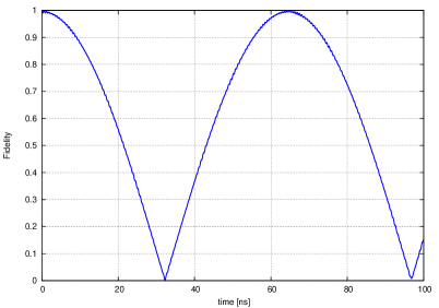
Refer to caption
Figure 10: Fidelity in the rotating frame as a function of time after unitary evolution of the state |0,0,0,0βŸ©β€‹|Ξ¦+βŸ©β€‹|𝟎,𝟎⟩ket0000ketsuperscriptΞ¦ket00|0,0,0,0\rangle|\Phi^{+}\rangle|\mathbf{0},\mathbf{0}\rangle and subsequently obtaining error syndrome (1,1)11(1,1). Parameters as in Figure (3). Compare to Figure (7).
FR​(|Ξ¦+⟩,ρqR)=⟨Φ+|ρqR|Ξ¦+⟩subscript𝐹𝑅ketsuperscriptΞ¦subscriptsuperscriptπœŒπ‘…π‘žquantum-operator-productsuperscriptΞ¦subscriptsuperscriptπœŒπ‘…π‘žsuperscriptΞ¦\displaystyle F_{R}(|\Phi^{+}\rangle,\rho^{R}_{q})=\sqrt{\langle\Phi^{+}|\rho^{R}_{q}|\Phi^{+}\rangle}
=\displaystyle= {12​p​(1,1)​[βˆ‘k=010Ξ²kβˆ—β€‹(t)​βk​(t)+Ξ²27βˆ—β€‹(t)​β27​(t)+Ξ²~0βˆ—β€‹(t)​β~27​(t)+Ξ²~27βˆ—β€‹(t)​β~0​(t)]}1/2superscript12𝑝11delimited-[]superscriptsubscriptπ‘˜010subscriptsuperscriptπ›½π‘˜π‘‘subscriptπ›½π‘˜π‘‘subscriptsuperscript𝛽27𝑑subscript𝛽27𝑑subscriptsuperscript~𝛽0𝑑subscript~𝛽27𝑑subscriptsuperscript~𝛽27𝑑subscript~𝛽0𝑑12\displaystyle\left\{\frac{1}{2p(1,1)}\biggl{[}\sum_{k=0}^{10}\beta^{*}_{k}(t)\beta_{k}(t)+\beta^{*}_{27}(t)\beta_{27}(t)+\tilde{\beta}^{*}_{0}(t)\tilde{\beta}_{27}(t)+\tilde{\beta}^{*}_{27}(t)\tilde{\beta}_{0}(t)\biggr{]}\right\}^{1/2}
=\displaystyle= {12​p​(1,1)​[βˆ‘k=010Ξ²kβˆ—β€‹(t)​βk​(t)+Ξ²27βˆ—β€‹(t)​β27​(t)+ei​ω+​t​β0βˆ—β€‹(t)​β27​(t)+eβˆ’i​ω+​t​β27βˆ—β€‹(t)​β0​(t)]}1/2,superscript12𝑝11delimited-[]superscriptsubscriptπ‘˜010subscriptsuperscriptπ›½π‘˜π‘‘subscriptπ›½π‘˜π‘‘subscriptsuperscript𝛽27𝑑subscript𝛽27𝑑superscript𝑒𝑖subscriptπœ”π‘‘subscriptsuperscript𝛽0𝑑subscript𝛽27𝑑superscript𝑒𝑖subscriptπœ”π‘‘subscriptsuperscript𝛽27𝑑subscript𝛽0𝑑12\displaystyle\left\{\frac{1}{2p(1,1)}\biggl{[}\sum_{k=0}^{10}\beta^{*}_{k}(t)\beta_{k}(t)+\beta^{*}_{27}(t)\beta_{27}(t)+e^{i\omega_{+}t}\beta^{*}_{0}(t)\beta_{27}(t)+e^{-i\omega_{+}t}\beta^{*}_{27}(t)\beta_{0}(t)\biggr{]}\right\}^{1/2},

as shown in Figure (10). It is readily verified that the relation between probalility for finding result (1,1)11(1,1) after re-insertion into the stabilizer and fidelity (70) is also valid in the rotating frame:

p~R​(1,1)=F2​(|Ξ¦+⟩,ρqR).subscript~𝑝𝑅11superscript𝐹2ketsuperscriptΞ¦subscriptsuperscriptπœŒπ‘…π‘ž\tilde{p}_{R}(1,1)=F^{2}(|\Phi^{+}\rangle,\rho^{R}_{q}). (109)

Analogous computations for the error syndrome (1,βˆ’1)11(1,-1) yield a modification of the fidelity (61) as well

FR​(|Ξ¦+⟩,X[2]​ρqR​X[2])=⟨Φ+|X[2]​ρqR​X[2]|Ξ¦+⟩=⟨Ψ+|ρq|Ξ¨+⟩subscript𝐹𝑅ketsuperscriptΞ¦superscript𝑋delimited-[]2subscriptsuperscriptπœŒπ‘…π‘žsuperscript𝑋delimited-[]2quantum-operator-productsuperscriptΞ¦superscript𝑋delimited-[]2subscriptsuperscriptπœŒπ‘…π‘žsuperscript𝑋delimited-[]2superscriptΞ¦quantum-operator-productsuperscriptΞ¨subscriptπœŒπ‘žsuperscriptΞ¨\displaystyle F_{R}(|\Phi^{+}\rangle,X^{[2]}\rho^{R}_{q}X^{[2]})=\sqrt{\langle\Phi^{+}|X^{[2]}\rho^{R}_{q}X^{[2]}|\Phi^{+}\rangle}=\sqrt{\langle\Psi^{+}|\rho_{q}|\Psi^{+}\rangle}
=\displaystyle= {12​p​(1,βˆ’1)​[Ξ²29βˆ—β€‹(t)​β29​(t)+Ξ²31βˆ—β€‹(t)​β31​(t)+Ξ²~31βˆ—β€‹(t)​β~29​(t)+Ξ²~29βˆ—β€‹(t)​β~31​(t)]}1/2superscript12𝑝11delimited-[]subscriptsuperscript𝛽29𝑑subscript𝛽29𝑑subscriptsuperscript𝛽31𝑑subscript𝛽31𝑑subscriptsuperscript~𝛽31𝑑subscript~𝛽29𝑑subscriptsuperscript~𝛽29𝑑subscript~𝛽31𝑑12\displaystyle\left\{\frac{1}{2p(1,-1)}\biggl{[}\beta^{*}_{29}(t)\beta_{29}(t)+\beta^{*}_{31}(t)\beta_{31}(t)+\tilde{\beta}^{*}_{31}(t)\tilde{\beta}_{29}(t)+\tilde{\beta}^{*}_{29}(t)\tilde{\beta}_{31}(t)\biggr{]}\right\}^{1/2}
=\displaystyle= {12​p​(1,βˆ’1)​[Ξ²29βˆ—β€‹(t)​β29​(t)+Ξ²31βˆ—β€‹(t)​β31​(t)+eiβ€‹Ο‰βˆ’β€‹t​β31βˆ—β€‹(t)​β29​(t)+eβˆ’iβ€‹Ο‰βˆ’β€‹t​β29βˆ—β€‹(t)​β31​(t)]}1/2.superscript12𝑝11delimited-[]subscriptsuperscript𝛽29𝑑subscript𝛽29𝑑subscriptsuperscript𝛽31𝑑subscript𝛽31𝑑superscript𝑒𝑖subscriptπœ”π‘‘subscriptsuperscript𝛽31𝑑subscript𝛽29𝑑superscript𝑒𝑖subscriptπœ”π‘‘subscriptsuperscript𝛽29𝑑subscript𝛽31𝑑12\displaystyle\left\{\frac{1}{2p(1,-1)}\biggl{[}\beta^{*}_{29}(t)\beta_{29}(t)+\beta^{*}_{31}(t)\beta_{31}(t)+e^{i\omega_{-}t}\beta^{*}_{31}(t)\beta_{29}(t)+e^{-i\omega_{-}t}\beta^{*}_{29}(t)\beta_{31}(t)\biggr{]}\right\}^{1/2}.

This result is depicted in Figure (11). The final fidelities after having obtained the error syndromes (βˆ’1,1)11(-1,1) and (βˆ’1,βˆ’1)11(-1,-1) do not change in the rotating frame. The reason is that these expressions do not contain interference between Ξ²k​(t)subscriptπ›½π‘˜π‘‘\beta_{k}(t) functions with different indices kπ‘˜k.

Bell state |Ψ+⟩ketsuperscriptΨ|\Psi^{+}\rangle\\

The unitarily evolved state corresponding to the two qubit Bell state |Ψ+⟩ketsuperscriptΨ|\Psi^{+}\rangle reads in the rotating frame

|ψR​(t)⟩=R​(t)​|Οˆβ€‹(t)⟩=βˆ‘k=132Ξ³~k​(t)​|fk⟩.ketsubscriptπœ“π‘…π‘‘π‘…π‘‘ketπœ“π‘‘superscriptsubscriptπ‘˜132subscript~π›Ύπ‘˜π‘‘ketsubscriptπ‘“π‘˜|\psi_{R}(t)\rangle=R(t)|\psi(t)\rangle=\sum_{k=1}^{32}\tilde{\gamma}_{k}(t)|f_{k}\rangle. (111)

The measurement probabilities once more do not change because Ξ³~​(t)​γ~βˆ—β€‹(t)=γ​(t)β€‹Ξ³βˆ—β€‹(t)~𝛾𝑑superscript~𝛾𝑑𝛾𝑑superscript𝛾𝑑\tilde{\gamma}(t)\tilde{\gamma}^{*}(t)=\gamma(t)\gamma^{*}(t). The density matrix resulting from the error syndrome (1,βˆ’1)11(1,-1) has two interference terms and, as a consequence, it gets modified. Concomitantly, we obtain a modification of the fidelity (64):

FR​(|Ξ¨+⟩,ρqR)=⟨Ψ+|ρqR|Ξ¨+⟩subscript𝐹𝑅ketsuperscriptΞ¨subscriptsuperscriptπœŒπ‘…π‘žquantum-operator-productsuperscriptΞ¨subscriptsuperscriptπœŒπ‘…π‘žsuperscriptΞ¨\displaystyle F_{R}(|\Psi^{+}\rangle,\rho^{R}_{q})=\sqrt{\langle\Psi^{+}|\rho^{R}_{q}|\Psi^{+}\rangle}
=\displaystyle= 12​p​(1,βˆ’1)​[Ξ³29βˆ—β€‹(t)​γ29​(t)+Ξ³31βˆ—β€‹(t)​γ31​(t)+Ξ³~31βˆ—β€‹(t)​γ~29​(t)+Ξ³~29βˆ—β€‹(t)​γ~31​(t)]12𝑝11delimited-[]subscriptsuperscript𝛾29𝑑subscript𝛾29𝑑subscriptsuperscript𝛾31𝑑subscript𝛾31𝑑subscriptsuperscript~𝛾31𝑑subscript~𝛾29𝑑subscriptsuperscript~𝛾29𝑑subscript~𝛾31𝑑\displaystyle\sqrt{\frac{1}{2p(1,-1)}\biggl{[}\gamma^{*}_{29}(t)\gamma_{29}(t)+\gamma^{*}_{31}(t)\gamma_{31}(t)+\tilde{\gamma}^{*}_{31}(t)\tilde{\gamma}_{29}(t)+\tilde{\gamma}^{*}_{29}(t)\tilde{\gamma}_{31}(t)\biggr{]}}
=\displaystyle= 12​p​(1,βˆ’1)​[Ξ³29βˆ—β€‹(t)​γ29​(t)+Ξ³31βˆ—β€‹(t)​γ31​(t)+eiβ€‹Ο‰βˆ’β€‹t​γ31βˆ—β€‹(t)​γ29​(t)+eβˆ’iβ€‹Ο‰βˆ’β€‹t​γ29βˆ—β€‹(t)​γ31​(t)].12𝑝11delimited-[]subscriptsuperscript𝛾29𝑑subscript𝛾29𝑑subscriptsuperscript𝛾31𝑑subscript𝛾31𝑑superscript𝑒𝑖subscriptπœ”π‘‘subscriptsuperscript𝛾31𝑑subscript𝛾29𝑑superscript𝑒𝑖subscriptπœ”π‘‘subscriptsuperscript𝛾29𝑑subscript𝛾31𝑑\displaystyle\sqrt{\frac{1}{2p(1,-1)}\biggl{[}\gamma^{*}_{29}(t)\gamma_{29}(t)+\gamma^{*}_{31}(t)\gamma_{31}(t)+e^{i\omega_{-}t}\gamma^{*}_{31}(t)\gamma_{29}(t)+e^{-i\omega_{-}t}\gamma^{*}_{29}(t)\gamma_{31}(t)\biggr{]}}.

This result is shown in Figure (12). The relation between probability after re-insertion and fidelity is once again valid

p~R​(1,βˆ’1)=F2​(|Ξ¨+⟩,ρqR).subscript~𝑝𝑅11superscript𝐹2ketsuperscriptΞ¨subscriptsuperscriptπœŒπ‘…π‘ž\tilde{p}_{R}(1,-1)=F^{2}(|\Psi^{+}\rangle,\rho^{R}_{q}). (113)

The other fidelities do not contain interference terms and are therefore not changed in the rotating frame.
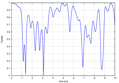
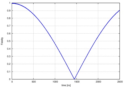
Refer to caption
Figure 11: Fidelity in the rotating frame as a function of time after unitary evolution of the state |0,0,0,0βŸ©β€‹|Ξ¦+βŸ©β€‹|𝟎,𝟎⟩ket0000ketsuperscriptΞ¦ket00|0,0,0,0\rangle|\Phi^{+}\rangle|\mathbf{0},\mathbf{0}\rangle, subsequently obtaining error syndrome (1,βˆ’1)11(1,-1) and error correction. Parameters as in Figure (3). Compare to Figure (8).
Refer to caption
Figure 12: Fidelity in the rotating frame as a function of time after unitary evolution of the state |0,0,0,0βŸ©β€‹|Ξ¨+βŸ©β€‹|𝟎,𝟎⟩ket0000ketsuperscriptΞ¨ket00|0,0,0,0\rangle|\Psi^{+}\rangle|\mathbf{0},\mathbf{0}\rangle and subsequently obtaining error syndrome result (1,βˆ’1)11(1,-1). Parameters as in Figure (3). Compare to Figure (9).

VI.2.2 Including ancillas

It is straightforward to extend the rotating frame with the ancillas. Their β€˜free’ Hamiltonians commute and they also commute with H0[12]superscriptsubscript𝐻0delimited-[]12H_{0}^{[12]}. If we denote the extended operator as β„›β„›\mathcal{R}, we obtain

ℛ​(t)​|fk⟩=ei​(Ο΅k[1]+Ο΅k[2]+Ο΅k[a]+Ο΅k[b])​t​|fk⟩,ℛ𝑑ketsubscriptπ‘“π‘˜superscript𝑒𝑖superscriptsubscriptitalic-Ο΅π‘˜delimited-[]1superscriptsubscriptitalic-Ο΅π‘˜delimited-[]2superscriptsubscriptitalic-Ο΅π‘˜delimited-[]π‘Žsuperscriptsubscriptitalic-Ο΅π‘˜delimited-[]𝑏𝑑ketsubscriptπ‘“π‘˜\mathcal{R}(t)|f_{k}\rangle=e^{i(\epsilon_{k}^{[1]}+\epsilon_{k}^{[2]}+\epsilon_{k}^{[a]}+\epsilon_{k}^{[b]})t}|f_{k}\rangle, (114)

with Ο΅k[a]=Β±12​ωa,Ο΅k[b]=Β±12​ωbformulae-sequencesuperscriptsubscriptitalic-Ο΅π‘˜delimited-[]π‘Žplus-or-minus12subscriptπœ”π‘Žsuperscriptsubscriptitalic-Ο΅π‘˜delimited-[]𝑏plus-or-minus12subscriptπœ”π‘\epsilon_{k}^{[a]}=\pm\tfrac{1}{2}\omega_{a},\epsilon_{k}^{[b]}=\pm\tfrac{1}{2}\omega_{b}, once more depending on the index kπ‘˜k. The relevant energies are given by

Ο΅0[1]+Ο΅0[2]=βˆ’12​ω+βˆ’12​ωaβˆ’12​ωb,superscriptsubscriptitalic-Ο΅0delimited-[]1superscriptsubscriptitalic-Ο΅0delimited-[]212subscriptπœ”12subscriptπœ”π‘Ž12subscriptπœ”π‘\displaystyle\epsilon_{0}^{[1]}+\epsilon_{0}^{[2]}=-\tfrac{1}{2}\omega_{+}-\tfrac{1}{2}\omega_{a}-\tfrac{1}{2}\omega_{b},
Ο΅27[1]+Ο΅27[2]=12β€‹Ο‰βˆ’βˆ’12​ωaβˆ’12​ωb,superscriptsubscriptitalic-Ο΅27delimited-[]1superscriptsubscriptitalic-Ο΅27delimited-[]212subscriptπœ”12subscriptπœ”π‘Ž12subscriptπœ”π‘\displaystyle\epsilon_{27}^{[1]}+\epsilon_{27}^{[2]}=\tfrac{1}{2}\omega_{-}-\tfrac{1}{2}\omega_{a}-\tfrac{1}{2}\omega_{b},
Ο΅29[1]+Ο΅29[2]=12β€‹Ο‰βˆ’βˆ’12​ωa+12​ωb,superscriptsubscriptitalic-Ο΅29delimited-[]1superscriptsubscriptitalic-Ο΅29delimited-[]212subscriptπœ”12subscriptπœ”π‘Ž12subscriptπœ”π‘\displaystyle\epsilon_{29}^{[1]}+\epsilon_{29}^{[2]}=\tfrac{1}{2}\omega_{-}-\tfrac{1}{2}\omega_{a}+\tfrac{1}{2}\omega_{b},
Ο΅31[1]+Ο΅31[2]=βˆ’12β€‹Ο‰βˆ’βˆ’12​ωa+12​ωb.superscriptsubscriptitalic-Ο΅31delimited-[]1superscriptsubscriptitalic-Ο΅31delimited-[]212subscriptπœ”12subscriptπœ”π‘Ž12subscriptπœ”π‘\displaystyle\epsilon_{31}^{[1]}+\epsilon_{31}^{[2]}=-\tfrac{1}{2}\omega_{-}-\tfrac{1}{2}\omega_{a}+\tfrac{1}{2}\omega_{b}. (115)

The functions Ξ²k​(t)subscriptπ›½π‘˜π‘‘\beta_{k}(t) and Ξ³k​(t)subscriptπ›Ύπ‘˜π‘‘\gamma_{k}(t) are now modified as

Ξ²^k​(t)subscript^π›½π‘˜π‘‘\displaystyle\hat{\beta}_{k}(t) =\displaystyle= ei​(Ο΅k[1]+Ο΅k[2]+Ο΅k[a]+Ο΅k[b])​t​βk​(t),superscript𝑒𝑖superscriptsubscriptitalic-Ο΅π‘˜delimited-[]1superscriptsubscriptitalic-Ο΅π‘˜delimited-[]2superscriptsubscriptitalic-Ο΅π‘˜delimited-[]π‘Žsuperscriptsubscriptitalic-Ο΅π‘˜delimited-[]𝑏𝑑subscriptπ›½π‘˜π‘‘\displaystyle e^{i(\epsilon_{k}^{[1]}+\epsilon_{k}^{[2]}+\epsilon_{k}^{[a]}+\epsilon_{k}^{[b]})t}\beta_{k}(t),
Ξ³^k​(t)subscript^π›Ύπ‘˜π‘‘\displaystyle\hat{\gamma}_{k}(t) =\displaystyle= ei​(Ο΅k[1]+Ο΅k[2]+Ο΅k[a]+Ο΅k[b])​t​γk​(t).superscript𝑒𝑖superscriptsubscriptitalic-Ο΅π‘˜delimited-[]1superscriptsubscriptitalic-Ο΅π‘˜delimited-[]2superscriptsubscriptitalic-Ο΅π‘˜delimited-[]π‘Žsuperscriptsubscriptitalic-Ο΅π‘˜delimited-[]𝑏𝑑subscriptπ›Ύπ‘˜π‘‘\displaystyle e^{i(\epsilon_{k}^{[1]}+\epsilon_{k}^{[2]}+\epsilon_{k}^{[a]}+\epsilon_{k}^{[b]})t}\gamma_{k}(t). (116)

The calculation now proceeds as above but now with the functions Ξ²^k​(t)subscript^π›½π‘˜π‘‘\hat{\beta}_{k}(t) and Ξ³^k​(t)subscript^π›Ύπ‘˜π‘‘\hat{\gamma}_{k}(t). The new phase factors due to the ancillas, however, cancel in the terms which could have altered the previous results for the fidelities. As a consequence, the obtained fidelities do not change in this extended rotated frame.

VII Theoretical discussion

VII.1 Error analysis

The stabilizing circuit with two ancilla qubits and two data qubits is a building block in surface codes for error correction Fowler ; Brav ; Terhal . Of course, this has motivated our choice for these investigations. The circuit, including the ancilla measurement and possibly error correction can deal with errors on the data qubits which occur before performing the circuit. The unitary evolution we have analyzed is supposed to take place between the circuit unitary operations and ancilla measurements. Even if one would be able to interpret the consequences as β€˜errors’, it is shown that they cannot be corrected in the usual way, that is applying the usual transformation on the data qubits based on the error syndromes.

With respect to the interpretation as β€˜errors’, there is no obvious identification of the error type. In Devitt coherent gate errors, environmental decoherence, initialization and measurement errors as well as loss and leakage are discussed. One may consider the electromagnetic resonators and even the ancillas as β€˜environment’; the ancillas are measured, the remaining resonators are traced out. It will be further analyzed below using the concept of quantum operations NC ; Caves . At this point, we can already state that it does not yield a satisfactory correction mechanism. Our findings are more similar to those in gate-error , where a gate-error analysis for transmon qubits is presented. The unitary evolution of the total system is also calculated in that study. As in our case, it is inherently unitary but yields detrimental effects on gates in the computational subspace. The β€˜errors’ are also systematic but appear incoherent in that subspace. In both analyses, they originate from entanglement with other states due to Hamiltonian evolution; in gate-error noncomputational transmon states and the resonator – in our work, ancillas and resonators.

Although no quantum code for the stabilizing circuit is developed as such, there is a certain resemblance because of the use of certain subspaces in a larger Hilbert space. Quantum error correction by means of coding, e.g. Shor’s nine-bit code, is for instance explained in Caves . Within a complete Hilbert space a code subspace is defined. The considered error operators map the code subspace to orthogonal subspaces. Errors can then be detected, distinguished and eventually corrected by determining in which subspace the system is. It can be done without disturbance and destroying the coherence; superposition and entanglement are essential in the process. Returning to the stabilizing circuit, we recall that a product state of a general two-data qubit state and the ancillas in the ground state is put in. The initial subspace is therefore four-dimensional, whereas the complete qubit Hilbert space is sixteen-dimensional. After the defined operations, the final state also belongs to a four-dimensional subspace, having the specific structure given in appendix B. The ancilla measurements subsequently project to one of the one-dimensional subspaces of the data qubit Hilbert space. However, if the final state evolves unitarily according to the system Hamiltonian then the four-dimensional subspace is abandoned. It explains why this particular error identification and correction does not work. Assume that the initial state is one of the Bell states. Without evolution the corresponding probabilities for the measurement outcomes are zero or one. This is no longer true after unitary evolution. Two more aspects are important. First, even if the ancilla measurement indicates no error, the final data qubit state is not the expected one. Secondly, if the syndrome indicates an error, the usual error correction transformations, cf. section II.2, do not work. Note that these findings do not depend merely on the inclusion of the resonators as degrees of freedom. Indeed, in a model with only spin-exchange interaction between adjacent qubits, similar results have been obtained spinstab . Of course, in the model with resonators one has to extend the ideal qubit state with resonators; here we have taken a product state with empty resonators. There remains a noticeable difference in the results compared to the spin model. Since a final data qubit state has to be identified the resonators have to be traced out after the evolution; it does not matter whether this is done before or after the measurement, see VII.3. In any case, the final data qubit β€˜state’ is not a pure state -as in the exchange model- but can only be described by means of a density operator. In both models, however, the essential phenomenon is that the evolution operator leads the state out of the stable subspace.

VII.2 Stabilizers in the Heisenberg picture

The concept of the X,Z𝑋𝑍X,Z stabilizing circuit has also been demonstrated by calculating with stabilizers instead of states Fowler . To this end, the Heisenberg representation is used. In particular, it is necessary to perform CNOT operations on products of the X𝑋X, Z𝑍Z and ℐℐ\mathcal{I} operators. Here we do not reproduce the derivation of appendix B of Fowler , but only note that the resulting two stabilizers are X[a]​X[1]​X[2]​ℐ[b]superscript𝑋delimited-[]π‘Žsuperscript𝑋delimited-[]1superscript𝑋delimited-[]2superscriptℐdelimited-[]𝑏X^{[a]}X^{[1]}X^{[2]}\mathcal{I}^{[b]} and ℐ[a]​Z[1]​Z[2]​Z[b]superscriptℐdelimited-[]π‘Žsuperscript𝑍delimited-[]1superscript𝑍delimited-[]2superscript𝑍delimited-[]𝑏\mathcal{I}^{[a]}Z^{[1]}Z^{[2]}Z^{[b]}. These operators commute and ancilla measurements indeed yield the two-qubit stabilizers Z[1]​Z[2]superscript𝑍delimited-[]1superscript𝑍delimited-[]2Z^{[1]}Z^{[2]} and X[1]​X[2]superscript𝑋delimited-[]1superscript𝑋delimited-[]2X^{[1]}X^{[2]}. However, in case of unitary evolution before the measurement we need to evolve the four-qubit stabilizers since we are in the Heisenberg representation. Without doing the explicit calculation, it is easily seen that the two stabilizers are not invariant under time-evolution. Recalling that in the Heisenberg equation for an operator A𝐴A the commutator [A,H]𝐴𝐻[A,H] drives non-trivial evolution, the commutators of the two four-qubit stabilizers with the full Hamiltonian are to be calculated. Here we only note that these commutators are nonzero causing the stabilizers to change. Equivalently, this can be seen using the explicitly constructed evolution operator U​(t)π‘ˆπ‘‘U(t) to find the evolution A​(t)=U​(t)​A​U†​(t)π΄π‘‘π‘ˆπ‘‘π΄superscriptπ‘ˆβ€ π‘‘A(t)=U(t)AU^{\dagger}(t). Once again, without doing the computation completely, it is clear that the stabilizers evolve non-trivially. As a consequence, the stabilizing mechanism will fail after finite time t𝑑t. Resonator operators will appear in the evolution of the stabilizers. After the evolution time t𝑑t they need to be traced out gain. The latter does of course not apply to the interacting spin system spinstab . Nevertheless, the stabilizers also evolve in time, reflecting the degradation of the stabilizer formalism taking into account full Hamiltonian evolution.

In larger systems on which a surface code can be implemented similar observations hold. Consider, for example, Surface 17 Versluis , which contains the studied two data qubits, two ancillas sytem as subsystems. Surface 17 consists out of nine data qubits and eight ancillas. In this system, eight stabilizers can be identified Fowler . These constrain the 29superscript292^{9}-dimensional data qubit space to a large extent. However, a two-dimensional subspace is not constrained. It can be exploited as computational space spanned by two logical qubits |πŸŽπ‹βŸ©,|πŸπ‹βŸ©ketsubscript0𝐋ketsubscript1𝐋|{\bf 0_{L}}\rangle,|{\bf 1_{L}}\rangle. Concomitantly, logical operators ZL,XLsubscript𝑍𝐿subscript𝑋𝐿Z_{L},X_{L} can be defined. Our concerns based on unitary evolution describing the complete dynamics apply here as well. Stabilizers and logical operators evolve in time and the associated subspaces are not invariant. Recently, a numerical study testing quantum fault tolerance on small systems has appeared Will .

VII.3 Quantum operations

The framework of quantum operations has been developed to deal with quantum noise by means of error correction NC ; Caves . The eventual error correction is typically done for the code subspace which, of course, is defined for a specific code. For example the three qubit bit flip code uses the two-dimensional code subspace spanned by the states |000⟩ket000|000\rangle and |111⟩ket111|111\rangle. The formalism aims at taking into account the interaction of the system of interest and the environment. It includes selective dynamics, where the environment is not observed, as well as nonselective dynamics, where a measurement on the environment is made. Various approaches for formulating quantum operations are presented in NC .

Here we use quantum operations to describe the processes in our system. Note that we do not consider a quantum code and, consequently, there is no code subspace. Noise is not considered and, concomitantly, there is no actual environment. We may, however, consider or rather describe the electromagnetic resonators as environment since we eventually focus on the qubits by taking the partial trace with respect to these degrees of freedom. Because the resonators are not measured, this dynamics is nonselective. In addition, the ancillas can be considered as environment as well. The reason is that they are measured also implying that their dynamics is selective. We will see below that the order of tracing out resonators and measuring the ancillas is not relevant.

Quantum operations are defined as operators transforming density matrices. For the full system we merely use the symbol ρ𝜌\rho, for data qubits ρqsubscriptπœŒπ‘ž\rho_{q}, for ancillas ρasubscriptπœŒπ‘Ž\rho_{a} and for resonators ρrsubscriptπœŒπ‘Ÿ\rho_{r}. The ideal circuit has the transformation property

|bmβŸ©β€‹| 0,πŸŽβŸ©β€‹βŸ¨bm|β€‹βŸ¨πŸŽ,𝟎|⟢|bmβŸ©β€‹|amβŸ©β€‹βŸ¨am|β€‹βŸ¨bm|,⟢ketsubscriptπ‘π‘šket 00brasubscriptπ‘π‘šbra00ketsubscriptπ‘π‘šketsubscriptπ‘Žπ‘šbrasubscriptπ‘Žπ‘šbrasubscriptπ‘π‘š|b_{m}\rangle|\,\mathbf{0,0}\rangle\langle b_{m}|\langle\mathbf{0,0}\,|\;\longrightarrow\;|b_{m}\rangle|a_{m}\rangle\langle a_{m}|\langle b_{m}|, (117)

where |bm⟩,m∈{1,2,3,4}ketsubscriptπ‘π‘šπ‘š1234|b_{m}\rangle,m\in\{1,2,3,4\} denotes one of the Bell states with corresponding ancilla state |am⟩ketsubscriptπ‘Žπ‘š|a_{m}\rangle. Next we extend this matrix with empty resonators thereby defining the initial density matrix before unitary evolution

ρ​(0)𝜌0\displaystyle\rho(0) =\displaystyle= |0,0,0,0βŸ©β€‹|bmβŸ©β€‹|amβŸ©β€‹βŸ¨am|β€‹βŸ¨bm|β€‹βŸ¨0,0,0,0|ket0000ketsubscriptπ‘π‘šketsubscriptπ‘Žπ‘šbrasubscriptπ‘Žπ‘šbrasubscriptπ‘π‘šbra0000\displaystyle|0,0,0,0\rangle|b_{m}\rangle|a_{m}\rangle\langle a_{m}|\langle b_{m}|\langle 0,0,0,0| (118)
=\displaystyle= ρr​(0)βŠ—Οq​(0)βŠ—Οa​(0).tensor-producttensor-productsubscriptπœŒπ‘Ÿ0subscriptπœŒπ‘ž0subscriptπœŒπ‘Ž0\displaystyle\rho_{r}(0)\otimes\rho_{q}(0)\otimes\rho_{a}(0).

Unitary evolution yields the density matrix

ρ​(t)=U​(t)​(ρr​(0)βŠ—Οq​(0)βŠ—Οa​(0))​U†​(t).πœŒπ‘‘π‘ˆπ‘‘tensor-producttensor-productsubscriptπœŒπ‘Ÿ0subscriptπœŒπ‘ž0subscriptπœŒπ‘Ž0superscriptπ‘ˆβ€ π‘‘\rho(t)=U(t)\left(\rho_{r}(0)\otimes\rho_{q}(0)\otimes\rho_{a}(0)\right)U^{\dagger}(t). (119)

Note that we explicitly have constructed the evolution operator up to (and including) the second excitation level. Measuring the ancillas is decribed by the operators Pksubscriptπ‘ƒπ‘˜P_{k} where k=(1,1)​…​(βˆ’1,βˆ’1)π‘˜11…11k=(1,1)\dots(-1,-1) labels the measurement result, i.e., the error syndrome. The subsequent β€˜amputation’ of the projected ancilla state can formally be done via a partial trace. Finally we trace out the resonators to obtain the quantum operation

ρq​(0)subscriptπœŒπ‘ž0\displaystyle\rho_{q}(0) β†’β†’\displaystyle\rightarrow ρq​(t)=ℰ​(ρq)subscriptπœŒπ‘žπ‘‘β„°subscriptπœŒπ‘ž\displaystyle\rho_{q}(t)=\mathcal{E}(\rho_{q})
=\displaystyle= trr​[tra​[Pk​U​(t)​(ρr​(0)βŠ—Οq​(0)βŠ—Οa​(0))​U†​Pk]].subscripttrπ‘Ÿdelimited-[]subscripttrπ‘Ždelimited-[]subscriptπ‘ƒπ‘˜π‘ˆπ‘‘tensor-producttensor-productsubscriptπœŒπ‘Ÿ0subscriptπœŒπ‘ž0subscriptπœŒπ‘Ž0superscriptπ‘ˆβ€ subscriptπ‘ƒπ‘˜\displaystyle\text{tr}_{r}\left[\text{tr}_{a}\left[P_{k}U(t)\left(\rho_{r}(0)\otimes\rho_{q}(0)\otimes\rho_{a}(0)\right)U^{\dagger}P_{k}\right]\right].

Alternatively, we take the partial trace with respect to the resonators before the measurement

ρ~q​(0)subscript~πœŒπ‘ž0\displaystyle\tilde{\rho}_{q}(0) β†’β†’\displaystyle\rightarrow ρ~q​(t)=β„°~​(ρq)subscript~πœŒπ‘žπ‘‘~β„°subscriptπœŒπ‘ž\displaystyle\tilde{\rho}_{q}(t)=\tilde{\mathcal{E}}(\rho_{q})
=\displaystyle= tra​[Pk​trr​[U​(t)​(ρr​(0)βŠ—Οq​(0)βŠ—Οa​(0))​U†]​Pk].subscripttrπ‘Ždelimited-[]subscriptπ‘ƒπ‘˜subscripttrπ‘Ÿdelimited-[]π‘ˆπ‘‘tensor-producttensor-productsubscriptπœŒπ‘Ÿ0subscriptπœŒπ‘ž0subscriptπœŒπ‘Ž0superscriptπ‘ˆβ€ subscriptπ‘ƒπ‘˜\displaystyle\text{tr}_{a}\left[P_{k}\,\text{tr}_{r}\left[U(t)\left(\rho_{r}(0)\otimes\rho_{q}(0)\otimes\rho_{a}(0)\right)U^{\dagger}\right]P_{k}\right].

Inserting the initial density matrix yields

ℰ​(ρq)=β„°~​(ρq)=βˆ‘rAk​r​ρq​Ak​r†,β„°subscriptπœŒπ‘ž~β„°subscriptπœŒπ‘žsubscriptπ‘Ÿsubscriptπ΄π‘˜π‘ŸsubscriptπœŒπ‘žsubscriptsuperscriptπ΄β€ π‘˜π‘Ÿ\mathcal{E}(\rho_{q})=\tilde{\mathcal{E}}(\rho_{q})=\sum_{r}A_{kr}\rho_{q}A^{\dagger}_{kr}, (122)

with the data qubit operators

Ak​r=⟨r​ak|U​(t)|r0​am⟩.subscriptπ΄π‘˜π‘Ÿquantum-operator-productπ‘Ÿsubscriptπ‘Žπ‘˜π‘ˆπ‘‘subscriptπ‘Ÿ0subscriptπ‘Žπ‘šA_{kr}=\langle ra_{k}|U(t)|r_{0}a_{m}\rangle. (123)

The resonator states are here denoted by |r⟩ketπ‘Ÿ|r\rangle and |r0⟩=|0,0,0,0⟩ketsubscriptπ‘Ÿ0ket0000|r_{0}\rangle=|0,0,0,0\rangle. The result generalizes the simplest operator-sum representation NC , because of the additional trace over the resonators. Its normalized form is given by

ℰ​(ρq)=βˆ‘rAk​r​ρq​Ak​r†tr​[βˆ‘rAk​r​ρq​Ak​r†],β„°subscriptπœŒπ‘žsubscriptπ‘Ÿsubscriptπ΄π‘˜π‘ŸsubscriptπœŒπ‘žsubscriptsuperscriptπ΄β€ π‘˜π‘Ÿtrdelimited-[]subscriptπ‘Ÿsubscriptπ΄π‘˜π‘ŸsubscriptπœŒπ‘žsubscriptsuperscriptπ΄β€ π‘˜π‘Ÿ\mathcal{E}(\rho_{q})=\frac{\sum_{r}A_{kr}\rho_{q}A^{\dagger}_{kr}}{\text{tr}\left[\sum_{r}A_{kr}\rho_{q}A^{\dagger}_{kr}\right]}, (124)

where the normalization equals the probability that the measurement outcome labelled kπ‘˜k is obtained for the defined initial Bell state. The operators A𝐴A, often denoted by E𝐸E, are called operational elements in NC ; in our case they depend on the evolution time. The theory of quantum error correction exploits these operators to derive conditions for error correction on a subspace defined by a certain quantum code NC . Note that in our case error correction would mean reversing the unitary evolution for the data qubits. Since this appears to be unfeasible in practice, we do not pursue this.

We conclude this section by noting that we have already derived explicit expressions for the quantum operations (124). For the initial Bell state |Ξ¦+⟩ketsuperscriptΞ¦|\Phi^{+}\rangle they are given in (IV.1), (IV.1), (60) and (62). The trivial, i.e., time-independent pure computational basis state, result (62) can be easily β€˜corrected’ because

CN​(𝑯[1]βŠ—β„[2])​| 0,𝟎⟩=|Ξ¦+⟩,subscript𝐢𝑁tensor-productsuperscript𝑯delimited-[]1superscriptℐdelimited-[]2ket 00ketsuperscriptΞ¦C_{N}\,\left(\bm{H}^{[1]}\otimes\mathcal{I}^{[2]}\right)|\,\mathbf{0,0}\rangle=|\Phi^{+}\rangle, (125)

where 𝑯𝑯\bm{H} is the Hadamard transformation and CNsubscript𝐢𝑁C_{N} denotes the CNOT operation.

VII.4 Synopsis

At this point, it may be useful to summarize the results of our study. First, we have computed unitary evolutions of the extended output states of the stabilized circuit. The extension is to include the empty resonators. For free evolution, i.e., zero couplings, the error syndrome indicating no error is obtained with certainty. This does not longer hold for the interacting case, where these probabilities become somewhat smaller than one. Concomitantly, the probabilities for a different syndrome which indicates an error are nonzero. The measurement operator for the error syndrome indicating no error does in general not project the evolved state on the desired target two-qubit resonator state. The exception is the case where the initial state is an eigenstate of the Hamiltonian which governs the time evolution. There are two related consequences. Calculating the fidelity of the two-qubit subsystem with the target Bell states, which is done by taking the partial trace of the resonator degrees of freedom, yields oscillating fidelities with high frequencies. Secondly, re-inserting the evolved two-qubit resonator stated completed with (possibly) re-initialized ancillas in the ground state, does not lead to the desired target state. The concomitant measurement probabilities resonate once again with high frequencies.

Similar results follow for error-corrected two-qubit states constructed after the first error detection. Neither high fidelities nor subsequent desired measurement probabilities close to one are obtained. It happens for free as well as complete, that is including the interactions, evolution. In other words, Hamiltonian governed unitary evolution causes problems for the stabilizing circuit as the target states are no energy eigenstates. For free evolution, however, target states are linear superpositions of eigenstates and, as a consequence, the probability of getting the syndrome indicating no error remains one. In the interacting case, even the latter breaks down although the mentioned probability is close to one whereas the error detection probabilities are rather small. Another difference for nonzero coupling is the fact that the two-qubit subsystem can only be described with a density matrix which does not correspond to a pure state. This is a consequence of the entanglement of data qubits and the resonators, even after the measurement of the ancillas. For the noninteracting system, the two-qubit resonator system is described by a product state and taking the partial trace yields a density matrix which describes a pure state. In fact, the results for H0subscript𝐻0H_{0} can be obtained without invoking the density matrix formalism.

The calculations have also been done in the rotating frame of the data qubits. Measurement probabilities for the various error syndromes are not altered. The fidelities, however, do change. The observed time variations are slower, which indicates the expected cancellation of the highest frequency components. Nevertheless, with one exception, the resulting fidelities decrease rather fast. Extending the rotating frame with respect to the ancillas does not change the results.

VIII Conclusion

Our semi-analytical analysis of the X𝑋X and Z𝑍Z stabilizing circuit has revealed deteriorating consequences of unitary evolution of the complete, i.e., qubits and resonators, interacting system. Probabilities for error syndromes indicating no error, therefore ideally equal one, decrease to the range 0.992βˆ’0.9990.9920.9990.992-0.999. Fidelities of the augmented density matrices and the stable target state, also ideally one, oscillate between 00 and 111. After having obtained an error syndrome indicating an error, the usual error correction does not apply. The latter is a forteriori explained because unitary evolution does lead out of subspaces on which the usual error correction does work. The explanation in terms of the stabilizers of the circuits is that they are no longer conserved, i.e., evolve non-trivially governed by the complete Hamiltonian.

Several caveats should be kept in mind with respect to this research. We have only addressed part of the effects of unitary evolution, that is only in a time interval between the last unitary operation in the stabilizing circuit and the ancilla measurement. The latter is supposed to be perfect. It is also assumed that the circuit performs perfectly. The rotating wave approximation has been made in the interaction terms. Environmental decoherence is neglected. Only the four-qubit system has been considered, etc.

Nevertheless, we think that the results can be relevant for the further development of quantum error correction and fault-tolerant computation. Recall that these concepts rely on the applicability of some mathematical error model, like one-qubit Pauli channels NC . The latter cannot describe the deleterious effects on the computational subspace we have identified. The preliminary, somewhat discomforting, overall conclusion is that the existing stabilizer codes are not sufficient to handle the consequences of unitary evolution of coupled (transmon-like) qubit–resonator quantum systems.

Acknowledgments

The authors thank B.M. Terhal and B. Criger for stimulating discussions. This research is supported by the Early Research Programme of the Netherlands Organisation for Applied Scientific Research (TNO). Additional support from the Top Sector High Tech Systems and Materials is highly appreciated.

Appendix A Definitions and notation

Throughout this paper we adopt units with ℏ=1Planck-constant-over-2-pi1\hbar=1.

For the two data qubit system we use the following definition of the Bell states

|Φ±⟩=12​2​(|𝟎,𝟎⟩±|𝟏,𝟏⟩),ketsuperscriptΞ¦plus-or-minus122plus-or-minusket00ket11\displaystyle|\Phi^{\pm}\rangle=\tfrac{1}{2}\sqrt{2}\left(|\mathbf{0,0}\rangle\pm|\mathbf{1,1}\rangle\right),
|Ψ±⟩=12​2​(|𝟎,𝟏⟩±|𝟏,𝟎⟩).ketsuperscriptΞ¨plus-or-minus122plus-or-minusket01ket10\displaystyle|\Psi^{\pm}\rangle=\tfrac{1}{2}\sqrt{2}\left(|\mathbf{0,1}\rangle\pm|\mathbf{1,0}\rangle\right). (A.126)

The operators Οƒz[1],Οƒz[2],Οƒx[1]superscriptsubscriptπœŽπ‘§delimited-[]1superscriptsubscriptπœŽπ‘§delimited-[]2superscriptsubscript𝜎π‘₯delimited-[]1\sigma_{z}^{[1]},\sigma_{z}^{[2]},\sigma_{x}^{[1]} and Οƒx[2]superscriptsubscript𝜎π‘₯delimited-[]2\sigma_{x}^{[2]} are also respectively denoted by Z[1],Z[2],X[1],Z[2]superscript𝑍delimited-[]1superscript𝑍delimited-[]2superscript𝑋delimited-[]1superscript𝑍delimited-[]2Z^{[1]},Z^{[2]},X^{[1]},Z^{[2]}. The superindex refers to the qubit; for the ancillas the indices a,bπ‘Žπ‘a,b will be analogously used. Below we need the action of the X𝑋X-operators on the basis states

X[1]​|Ξ¦+⟩=|Ξ¨+⟩,superscript𝑋delimited-[]1ketsuperscriptΞ¦ketsuperscriptΞ¨\displaystyle X^{[1]}|\Phi^{+}\rangle=|\Psi^{+}\rangle, X[2]​|Ξ¦+⟩=|Ξ¨+⟩,superscript𝑋delimited-[]2ketsuperscriptΞ¦ketsuperscriptΞ¨\displaystyle X^{[2]}|\Phi^{+}\rangle=|\Psi^{+}\rangle,
X[1]​|Ξ¦βˆ’βŸ©=βˆ’|Ξ¨βˆ’βŸ©,superscript𝑋delimited-[]1ketsuperscriptΞ¦ketsuperscriptΞ¨\displaystyle X^{[1]}|\Phi^{-}\rangle=-|\Psi^{-}\rangle, X[2]​|Ξ¦βˆ’βŸ©=|Ξ¨βˆ’βŸ©,superscript𝑋delimited-[]2ketsuperscriptΞ¦ketsuperscriptΞ¨\displaystyle X^{[2]}|\Phi^{-}\rangle=|\Psi^{-}\rangle,
X[1]​|Ξ¨+⟩=|Ξ¦+⟩,superscript𝑋delimited-[]1ketsuperscriptΞ¨ketsuperscriptΞ¦\displaystyle X^{[1]}|\Psi^{+}\rangle=|\Phi^{+}\rangle, X[2]​|Ξ¨+⟩=|Ξ¦+⟩,superscript𝑋delimited-[]2ketsuperscriptΞ¨ketsuperscriptΞ¦\displaystyle X^{[2]}|\Psi^{+}\rangle=|\Phi^{+}\rangle,
X[1]​|Ξ¨βˆ’βŸ©=βˆ’|Ξ¦βˆ’βŸ©,superscript𝑋delimited-[]1ketsuperscriptΞ¨ketsuperscriptΞ¦\displaystyle X^{[1]}|\Psi^{-}\rangle=-|\Phi^{-}\rangle, X[2]​|Ξ¨βˆ’βŸ©=|Ξ¦βˆ’βŸ©.superscript𝑋delimited-[]2ketsuperscriptΞ¨ketsuperscriptΞ¦\displaystyle X^{[2]}|\Psi^{-}\rangle=|\Phi^{-}\rangle. (A.127)

Because we will consider a X𝑋X and Z𝑍Z stabilizer circuit, we apply the Z𝑍Z-operators to the Bell states as well and get

Z[1]​|Ξ¦+⟩=|Ξ¦βˆ’βŸ©,superscript𝑍delimited-[]1ketsuperscriptΞ¦ketsuperscriptΞ¦\displaystyle Z^{[1]}|\Phi^{+}\rangle=|\Phi^{-}\rangle, Z[2]​|Ξ¦+⟩=|Ξ¦βˆ’βŸ©,superscript𝑍delimited-[]2ketsuperscriptΞ¦ketsuperscriptΞ¦\displaystyle Z^{[2]}|\Phi^{+}\rangle=|\Phi^{-}\rangle,
Z[1]​|Ξ¦βˆ’βŸ©=|Ξ¦+⟩,superscript𝑍delimited-[]1ketsuperscriptΞ¦ketsuperscriptΞ¦\displaystyle Z^{[1]}|\Phi^{-}\rangle=|\Phi^{+}\rangle, Z[2]​|Ξ¦βˆ’βŸ©=|Ξ¦+⟩,superscript𝑍delimited-[]2ketsuperscriptΞ¦ketsuperscriptΞ¦\displaystyle Z^{[2]}|\Phi^{-}\rangle=|\Phi^{+}\rangle,
Z[1]​|Ξ¨+⟩=|Ξ¨βˆ’βŸ©,superscript𝑍delimited-[]1ketsuperscriptΞ¨ketsuperscriptΞ¨\displaystyle Z^{[1]}|\Psi^{+}\rangle=|\Psi^{-}\rangle, Z[2]​|Ξ¨+⟩=βˆ’|Ξ¨βˆ’βŸ©,superscript𝑍delimited-[]2ketsuperscriptΞ¨ketsuperscriptΞ¨\displaystyle Z^{[2]}|\Psi^{+}\rangle=-|\Psi^{-}\rangle,
Z[1]​|Ξ¨βˆ’βŸ©=|Ξ¨+⟩,superscript𝑍delimited-[]1ketsuperscriptΞ¨ketsuperscriptΞ¨\displaystyle Z^{[1]}|\Psi^{-}\rangle=|\Psi^{+}\rangle, Z[2]​|Ξ¨βˆ’βŸ©=βˆ’|Ξ¨+⟩.superscript𝑍delimited-[]2ketsuperscriptΞ¨ketsuperscriptΞ¨\displaystyle Z^{[2]}|\Psi^{-}\rangle=-|\Psi^{+}\rangle. (A.128)

A general two-qubit state, usually written as superposition of computational states, can also be written as a linear combination of the Bell states, i.e.,

|Ξ¨12⟩=A+​|Ξ¦+⟩+Aβˆ’β€‹|Ξ¦βˆ’βŸ©+B+​|Ξ¨+⟩+Bβˆ’β€‹|Ξ¨βˆ’βŸ©,ketsubscriptΞ¨12subscript𝐴ketsuperscriptΞ¦subscript𝐴ketsuperscriptΞ¦subscript𝐡ketsuperscriptΞ¨subscript𝐡ketsuperscriptΞ¨|\Psi_{12}\rangle=A_{+}|\Phi^{+}\rangle+A_{-}|\Phi^{-}\rangle+B_{+}|\Psi^{+}\rangle+B_{-}|\Psi^{-}\rangle, (A.129)

with |A+|2+|Aβˆ’|2+|B+|2+|Bβˆ’|2=1superscriptsubscript𝐴2superscriptsubscript𝐴2superscriptsubscript𝐡2superscriptsubscript𝐡21|A_{+}|^{2}+|A_{-}|^{2}+|B_{+}|^{2}+|B_{-}|^{2}=1.

Appendix B Circuit analyis in terms of Bell states

In this appendix we also use the one-qubit states

|±⟩=12​2​(|𝟎⟩±|𝟏⟩).ketplus-or-minus122plus-or-minusket0ket1|\bm{\pm}\rangle=\tfrac{1}{2}\sqrt{2}\left(|\mathbf{0}\rangle\pm|\mathbf{1}\rangle\right). (B.1)

Recall that they are obtained via the Hadamard transformation on the computational states

𝑯​| 0⟩=|+⟩,𝑯​| 1⟩=|βˆ’βŸ©.formulae-sequence𝑯ket 0ket𝑯ket1ket\bm{H}|\,\mathbf{0}\rangle=|\bm{+}\rangle,\qquad\bm{H}|\,\mathbf{1}\rangle=|\bm{-}\rangle. (B.2)

We re-analyze the X𝑋X and Z𝑍Z stabilizing circuit in terms of Bell states, cf. Fowler . Explicitly the following steps are done:

  1. 1.

    Initialize both ancillas in their ground state. The data qubits are in a general state given in (A.129). Consequently the initial four-qubit state reads

    |ψ1⟩=| 0βŸ©β€‹(A+​|Ξ¦+⟩+Aβˆ’β€‹|Ξ¦βˆ’βŸ©+B+​|Ξ¨+⟩+Bβˆ’β€‹|Ξ¨βˆ’βŸ©)​| 0⟩.ketsubscriptπœ“1ket 0subscript𝐴ketsuperscriptΞ¦subscript𝐴ketsuperscriptΞ¦subscript𝐡ketsuperscriptΞ¨subscript𝐡ketsuperscriptΞ¨ket 0\displaystyle|\psi_{1}\rangle=|\,\mathbf{0}\rangle\left(A_{+}|\Phi^{+}\rangle+A_{-}|\Phi^{-}\rangle+B_{+}|\Psi^{+}\rangle+B_{-}|\Psi^{-}\rangle\right)|\,\mathbf{0}\rangle. (B.3)
  2. 2.

    Perform a Hadamard operation on ancilla A

    |ψ2⟩=|+βŸ©β€‹(A+​|Ξ¦+⟩+Aβˆ’β€‹|Ξ¦βˆ’βŸ©+B+​|Ξ¨+⟩+Bβˆ’β€‹|Ξ¨βˆ’βŸ©)​| 0⟩.ketsubscriptπœ“2ketsubscript𝐴ketsuperscriptΞ¦subscript𝐴ketsuperscriptΞ¦subscript𝐡ketsuperscriptΞ¨subscript𝐡ketsuperscriptΞ¨ket 0|\psi_{2}\rangle=|\bm{+}\rangle\left(A_{+}|\Phi^{+}\rangle+A_{-}|\Phi^{-}\rangle+B_{+}|\Psi^{+}\rangle+B_{-}|\Psi^{-}\rangle\right)|\,\mathbf{0}\rangle. (B.4)
  3. 3.

    With ancilla A as control and qubit 1 as target, a CNOT is applied:

    |ψ3⟩ketsubscriptπœ“3\displaystyle|\psi_{3}\rangle =\displaystyle= 122[| 0⟩(A+|Ξ¦+⟩+Aβˆ’|Ξ¦βˆ’βŸ©+B+|Ξ¨+⟩+Bβˆ’|Ξ¨βˆ’βŸ©)\displaystyle\tfrac{1}{2}\sqrt{2}[|\,\mathbf{0}\rangle\left(A_{+}|\Phi^{+}\rangle+A_{-}|\Phi^{-}\rangle+B_{+}|\Psi^{+}\rangle+B_{-}|\Psi^{-}\rangle\right) (B.5)
    +\displaystyle+ | 1⟩(A+|Ξ¨+βŸ©βˆ’Aβˆ’|Ξ¨βˆ’βŸ©+B+|Ξ¦+βŸ©βˆ’Bβˆ’|Ξ¦βˆ’βŸ©)]| 0⟩.\displaystyle|\,\mathbf{1}\rangle\left(A_{+}|\Psi^{+}\rangle-A_{-}|\Psi^{-}\rangle+B_{+}|\Phi^{+}\rangle-B_{-}|\Phi^{-}\rangle\right)]|\,\mathbf{0}\rangle.
  4. 4.

    A second CNOT is applied, again with ancilla A as control. Qubit 2, however, is the target:

    |ψ4⟩ketsubscriptπœ“4\displaystyle|\psi_{4}\rangle =\displaystyle= 122[| 0⟩(A+|Ξ¦+⟩+Aβˆ’|Ξ¦βˆ’βŸ©+B+|Ξ¨+⟩+Bβˆ’|Ξ¨βˆ’βŸ©)\displaystyle\tfrac{1}{2}\sqrt{2}[|\,\mathbf{0}\rangle\left(A_{+}|\Phi^{+}\rangle+A_{-}|\Phi^{-}\rangle+B_{+}|\Psi^{+}\rangle+B_{-}|\Psi^{-}\rangle\right)
    +\displaystyle+ | 1⟩(A+|Ξ¦+βŸ©βˆ’Aβˆ’|Ξ¦βˆ’βŸ©+B+|Ξ¨+βŸ©βˆ’Bβˆ’|Ξ¨βˆ’βŸ©)]| 0⟩\displaystyle|\,\mathbf{1}\rangle\left(A_{+}|\Phi^{+}\rangle-A_{-}|\Phi^{-}\rangle+B_{+}|\Psi^{+}\rangle-B_{-}|\Psi^{-}\rangle\right)]|\,\mathbf{0}\rangle
    =\displaystyle= |+⟩(A+|Ξ¦+⟩+B+|Ξ¨+⟩)| 0⟩+|βˆ’βŸ©(Aβˆ’|Ξ¦βˆ’βŸ©+Bβˆ’|Ξ¨βˆ’βŸ©)]| 0⟩.\displaystyle|\bm{+}\rangle\left(A_{+}|\Phi^{+}\rangle+B_{+}|\Psi^{+}\rangle\right)|\,\mathbf{0}\rangle+|\bm{-}\rangle\left(A_{-}|\Phi^{-}\rangle+B_{-}|\Psi^{-}\rangle\right)]|\,\mathbf{0}\rangle.
  5. 5.

    A CNOT is applied with data qubit 1 as control and ancilla B as target. We omit the intermediate result |ψ5⟩ketsubscriptπœ“5|\psi_{5}\rangle because it is more convenient to combine this operation with the next step.

  6. 6.

    A CNOT is applied with data qubit 2 as control and ancilla B as target. The two CNOTs yield for the relevant states

    |Ξ¦Β±βŸ©β€‹| 0βŸ©β†’|Ξ¦Β±βŸ©β€‹| 0⟩,|Ξ¨Β±βŸ©β€‹| 0βŸ©β†’|Ξ¨Β±βŸ©β€‹| 1⟩.formulae-sequenceβ†’ketsuperscriptΞ¦plus-or-minusket 0ketsuperscriptΞ¦plus-or-minusket 0β†’ketsuperscriptΞ¨plus-or-minusket 0ketsuperscriptΞ¨plus-or-minusket1|\Phi^{\pm}\rangle|\,\mathbf{0}\rangle\rightarrow|\Phi^{\pm}\rangle|\,\mathbf{0}\rangle,\quad|\Psi^{\pm}\rangle|\,\mathbf{0}\rangle\rightarrow|\Psi^{\pm}\rangle|\,\mathbf{1}\rangle. (B.7)

    Therefore, the resulting four-qubit state reads

    |ψ6⟩=A+​|+βŸ©β€‹|Ξ¦+βŸ©β€‹| 0⟩+B+​|+βŸ©β€‹|Ξ¨+βŸ©β€‹| 1⟩+Aβˆ’β€‹|βˆ’βŸ©β€‹|Ξ¦βˆ’βŸ©β€‹| 0⟩+Bβˆ’β€‹|βˆ’βŸ©β€‹|Ξ¨βˆ’βŸ©β€‹| 1⟩.ketsubscriptπœ“6subscript𝐴ketketsuperscriptΞ¦ket 0subscript𝐡ketketsuperscriptΞ¨ket1subscript𝐴ketketsuperscriptΞ¦ket 0subscript𝐡ketketsuperscriptΞ¨ket1|\psi_{6}\rangle=A_{+}|\bm{+}\rangle|\Phi^{+}\rangle|\,\mathbf{0}\rangle+B_{+}|\bm{+}\rangle|\Psi^{+}\rangle|\,\mathbf{1}\rangle+A_{-}|\bm{-}\rangle|\Phi^{-}\rangle|\,\mathbf{0}\rangle+B_{-}|\bm{-}\rangle|\Psi^{-}\rangle|\,\mathbf{1}\rangle. (B.8)
  7. 7.

    A Hadamard is performed on ancilla A; we obtain

    |ψ7⟩=A+​| 0βŸ©β€‹|Ξ¦+βŸ©β€‹| 0⟩+B+​| 0βŸ©β€‹|Ξ¨+βŸ©β€‹| 1⟩+Aβˆ’β€‹| 1βŸ©β€‹|Ξ¦βˆ’βŸ©β€‹| 0⟩+Bβˆ’β€‹| 1βŸ©β€‹|Ξ¨βˆ’βŸ©β€‹| 1⟩.ketsubscriptπœ“7subscript𝐴ket 0ketsuperscriptΞ¦ket 0subscript𝐡ket 0ketsuperscriptΞ¨ket1subscript𝐴ket1ketsuperscriptΞ¦ket 0subscript𝐡ket1ketsuperscriptΞ¨ket1|\psi_{7}\rangle=A_{+}|\,\mathbf{0}\rangle|\Phi^{+}\rangle|\,\mathbf{0}\rangle+B_{+}|\,\mathbf{0}\rangle|\Psi^{+}\rangle|\,\mathbf{1}\rangle+A_{-}|\,\mathbf{1}\rangle|\Phi^{-}\rangle|\,\mathbf{0}\rangle+B_{-}|\,\mathbf{1}\rangle|\Psi^{-}\rangle|\,\mathbf{1}\rangle. (B.9)
  8. 8.

    Both ancillas are eventually measured in their standard basis. The concomitant measurement operators are given by

    P11=| 0βŸ©β€‹βŸ¨πŸŽ|βŠ—β„12βŠ—| 0βŸ©β€‹βŸ¨πŸŽ|,subscript𝑃11tensor-productket 0bra0subscriptℐ12ket 0bra0\displaystyle P_{11}=|\,\mathbf{0}\rangle\langle\mathbf{0}\,|\otimes\mathcal{I}_{12}\otimes|\,\mathbf{0}\rangle\langle\mathbf{0}\,|, Pβˆ’11=| 1βŸ©β€‹βŸ¨πŸ|βŠ—β„12βŠ—| 0βŸ©β€‹βŸ¨πŸŽ|,subscript𝑃11tensor-productket1bra1subscriptℐ12ket 0bra0\displaystyle P_{-11}=|\,\mathbf{1}\rangle\langle\mathbf{1}\,|\otimes\mathcal{I}_{12}\otimes|\,\mathbf{0}\rangle\langle\mathbf{0}\,|,
    P1βˆ’1=| 0βŸ©β€‹βŸ¨πŸŽ|βŠ—β„12βŠ—| 1βŸ©β€‹βŸ¨πŸ|,subscript𝑃11tensor-productket 0bra0subscriptℐ12ket1bra1\displaystyle P_{1-1}=|\,\mathbf{0}\rangle\langle\mathbf{0}\,|\otimes\mathcal{I}_{12}\otimes|\,\mathbf{1}\rangle\langle\mathbf{1}\,|, Pβˆ’1βˆ’1=| 1βŸ©β€‹βŸ¨πŸ|βŠ—β„12βŠ—| 1βŸ©β€‹βŸ¨πŸ|,subscript𝑃11tensor-productket1bra1subscriptℐ12ket1bra1\displaystyle P_{-1-1}=|\,\mathbf{1}\rangle\langle\mathbf{1}\,|\otimes\mathcal{I}_{12}\otimes|\,\mathbf{1}\rangle\langle\mathbf{1}\,|, (B.10)

    with probabilities for the outcomes Β±1,Β±1plus-or-minus1plus-or-minus1\pm 1,\pm 1

    p​(1,1)=|A+|2,𝑝11superscriptsubscript𝐴2\displaystyle p(1,1)=|A_{+}|^{2}, p​(1,βˆ’1)=|B+|2,𝑝11superscriptsubscript𝐡2\displaystyle p(1,-1)=|B_{+}|^{2},
    p​(βˆ’1,1)=|Aβˆ’|2,𝑝11superscriptsubscript𝐴2\displaystyle p(-1,1)=|A_{-}|^{2}, p​(βˆ’1,βˆ’1)=|Bβˆ’|2.𝑝11superscriptsubscript𝐡2\displaystyle p(-1,-1)=|B_{-}|^{2}. (B.11)

    The corresponding final two-qubit states are the Bell states

    syndrome​(1,1):|Ξ¦+⟩,:syndrome11ketsuperscriptΞ¦\displaystyle\text{syndrome}\,(1,1):|\Phi^{+}\rangle, syndrome​(1,βˆ’1):|Ξ¨+⟩,:syndrome11ketsuperscriptΞ¨\displaystyle\text{syndrome}\,(1,-1):|\Psi^{+}\rangle,
    syndrome​(βˆ’1,1):|Ξ¦βˆ’βŸ©,:syndrome11ketsuperscriptΞ¦\displaystyle\text{syndrome}\,(-1,1):|\Phi^{-}\rangle, syndrome​(βˆ’1,βˆ’1):|Ξ¨βˆ’βŸ©.:syndrome11ketsuperscriptΞ¨\displaystyle\text{syndrome}\,(-1,-1):|\Psi^{-}\rangle. (B.12)

Appendix C Basis states and matrix elements

C.1 First excitation level

In this subspace, we choose the basis states

|e1⟩=|1,0,0,0βŸ©βŠ—|𝟎,πŸŽβŸ©βŠ—|𝟎,𝟎⟩,ketsubscript𝑒1tensor-productket1000ket00ket00\displaystyle|e_{1}\rangle=|1,0,0,0\rangle\otimes|\bm{0},\bm{0}\rangle\otimes|\bm{0},\bm{0}\rangle, |e2⟩=|0,1,0,0βŸ©βŠ—|𝟎,πŸŽβŸ©βŠ—|𝟎,𝟎⟩,ketsubscript𝑒2tensor-productket0100ket00ket00\displaystyle\quad|e_{2}\rangle=|0,1,0,0\rangle\otimes|\bm{0},\bm{0}\rangle\otimes|\bm{0},\bm{0}\rangle,
|e3⟩=|0,0,1,0βŸ©βŠ—|𝟎,πŸŽβŸ©βŠ—|𝟎,𝟎⟩,ketsubscript𝑒3tensor-productket0010ket00ket00\displaystyle|e_{3}\rangle=|0,0,1,0\rangle\otimes|\bm{0},\bm{0}\rangle\otimes|\bm{0},\bm{0}\rangle, |e4⟩=|0,0,0,1βŸ©βŠ—|𝟎,πŸŽβŸ©βŠ—|𝟎,𝟎⟩,ketsubscript𝑒4tensor-productket0001ket00ket00\displaystyle\quad|e_{4}\rangle=|0,0,0,1\rangle\otimes|\bm{0},\bm{0}\rangle\otimes|\bm{0},\bm{0}\rangle,
|e5⟩=|0,0,0,0βŸ©βŠ—|𝟏,πŸŽβŸ©βŠ—|𝟎,𝟎⟩,ketsubscript𝑒5tensor-productket0000ket10ket00\displaystyle|e_{5}\rangle=|0,0,0,0\rangle\otimes|\bm{1},\bm{0}\rangle\otimes|\bm{0},\bm{0}\rangle, |e6⟩=|0,0,0,0βŸ©βŠ—|𝟎,πŸβŸ©βŠ—|𝟎,𝟎⟩,ketsubscript𝑒6tensor-productket0000ket01ket00\displaystyle\quad|e_{6}\rangle=|0,0,0,0\rangle\otimes|\bm{0},\bm{1}\rangle\otimes|\bm{0},\bm{0}\rangle,
|e7⟩=|0,0,0,0βŸ©βŠ—|𝟎,πŸŽβŸ©βŠ—|𝟏,𝟎⟩,ketsubscript𝑒7tensor-productket0000ket00ket10\displaystyle|e_{7}\rangle=|0,0,0,0\rangle\otimes|\bm{0},\bm{0}\rangle\otimes|\bm{1},\bm{0}\rangle, |e8⟩=|0,0,0,0βŸ©βŠ—|𝟎,πŸŽβŸ©βŠ—|𝟎,𝟏⟩.ketsubscript𝑒8tensor-productket0000ket00ket01\displaystyle\quad|e_{8}\rangle=|0,0,0,0\rangle\otimes|\bm{0},\bm{0}\rangle\otimes|\bm{0},\bm{1}\rangle. (C.1)

The matrix elements of the Hamiltonian in this subspace can be readily calculated from

β„‹i​j=⟨ei|H|ej⟩,i,j=1,2,…​8.formulae-sequencesubscriptℋ𝑖𝑗quantum-operator-productsubscript𝑒𝑖𝐻subscript𝑒𝑗𝑖𝑗12…8\mathcal{H}_{ij}=\langle e_{i}|H|e_{j}\rangle,\qquad i,j=1,2,\dots 8. (C.2)

For i≀j𝑖𝑗i\leq j the nonzero elements are

β„‹11subscriptβ„‹11\displaystyle\mathcal{H}_{11} =\displaystyle= E0+Ο‰1,β„‹15=g11,β„‹17=g1​a,formulae-sequencesubscript𝐸0subscriptπœ”1subscriptβ„‹15subscript𝑔11subscriptβ„‹17subscript𝑔1π‘Ž\displaystyle E_{0}+\omega_{1},\quad\mathcal{H}_{15}=g_{11},\quad\mathcal{H}_{17}=g_{1a},
β„‹22subscriptβ„‹22\displaystyle\mathcal{H}_{22} =\displaystyle= E0+Ο‰2,β„‹26=g22,β„‹27=g2​a,formulae-sequencesubscript𝐸0subscriptπœ”2subscriptβ„‹26subscript𝑔22subscriptβ„‹27subscript𝑔2π‘Ž\displaystyle E_{0}+\omega_{2},\quad\mathcal{H}_{26}=g_{22},\quad\mathcal{H}_{27}=g_{2a},
β„‹33subscriptβ„‹33\displaystyle\mathcal{H}_{33} =\displaystyle= E0+Ο‰3,β„‹35=g31,β„‹38=g3​b,formulae-sequencesubscript𝐸0subscriptπœ”3subscriptβ„‹35subscript𝑔31subscriptβ„‹38subscript𝑔3𝑏\displaystyle E_{0}+\omega_{3},\quad\mathcal{H}_{35}=g_{31},\quad\mathcal{H}_{38}=g_{3b},
β„‹44subscriptβ„‹44\displaystyle\mathcal{H}_{44} =\displaystyle= E0+Ο‰4,β„‹46=g42,β„‹48=g4​b,formulae-sequencesubscript𝐸0subscriptπœ”4subscriptβ„‹46subscript𝑔42subscriptβ„‹48subscript𝑔4𝑏\displaystyle E_{0}+\omega_{4},\quad\mathcal{H}_{46}=g_{42},\quad\mathcal{H}_{48}=g_{4b}, (C.3)
β„‹55subscriptβ„‹55\displaystyle\mathcal{H}_{55} =\displaystyle= E0+Ο‰1β€²,β„‹66=E0+Ο‰2β€²,β„‹77=E0+Ο‰a,β„‹88=E0+Ο‰b,formulae-sequencesubscript𝐸0subscriptsuperscriptπœ”β€²1subscriptβ„‹66subscript𝐸0subscriptsuperscriptπœ”β€²2formulae-sequencesubscriptβ„‹77subscript𝐸0subscriptπœ”π‘Žsubscriptβ„‹88subscript𝐸0subscriptπœ”π‘\displaystyle E_{0}+\omega^{\prime}_{1},\quad\mathcal{H}_{66}=E_{0}+\omega^{\prime}_{2},\quad\mathcal{H}_{77}=E_{0}+\omega_{a},\quad\mathcal{H}_{88}=E_{0}+\omega_{b},

whereas the other ones follow by symmetry β„‹i​j=β„‹j​isubscriptℋ𝑖𝑗subscriptℋ𝑗𝑖\mathcal{H}_{ij}=\mathcal{H}_{ji}.

C.2 Second excitation level

We proceed to the second excitation level which has dimension thirty-two. Its basis is chosen as

|f1⟩=|2,0,0,0βŸ©βŠ—|𝟎,πŸŽβŸ©βŠ—|𝟎,𝟎⟩,ketsubscript𝑓1tensor-productket2000ket00ket00\displaystyle|f_{1}\rangle=|2,0,0,0\rangle\otimes|\bm{0},\bm{0}\rangle\otimes|\bm{0},\bm{0}\rangle, |f2⟩=|1,1,0,0βŸ©βŠ—|𝟎,πŸŽβŸ©βŠ—|𝟎,𝟎⟩,ketsubscript𝑓2tensor-productket1100ket00ket00\displaystyle\quad|f_{2}\rangle=|1,1,0,0\rangle\otimes|\bm{0},\bm{0}\rangle\otimes|\bm{0},\bm{0}\rangle,
|f3⟩=|1,0,1,0βŸ©βŠ—|𝟎,πŸŽβŸ©βŠ—|𝟎,𝟎⟩,ketsubscript𝑓3tensor-productket1010ket00ket00\displaystyle|f_{3}\rangle=|1,0,1,0\rangle\otimes|\bm{0},\bm{0}\rangle\otimes|\bm{0},\bm{0}\rangle, |f4⟩=|1,0,0,1βŸ©βŠ—|𝟎,πŸŽβŸ©βŠ—|𝟎,𝟎⟩,ketsubscript𝑓4tensor-productket1001ket00ket00\displaystyle\quad|f_{4}\rangle=|1,0,0,1\rangle\otimes|\bm{0},\bm{0}\rangle\otimes|\bm{0},\bm{0}\rangle,
|f5⟩=|0,2,0,0βŸ©βŠ—|𝟎,πŸŽβŸ©βŠ—|𝟎,𝟎⟩,ketsubscript𝑓5tensor-productket0200ket00ket00\displaystyle|f_{5}\rangle=|0,2,0,0\rangle\otimes|\bm{0},\bm{0}\rangle\otimes|\bm{0},\bm{0}\rangle, |f6⟩=|0,1,1,0βŸ©βŠ—|𝟎,πŸŽβŸ©βŠ—|𝟎,𝟎⟩,ketsubscript𝑓6tensor-productket0110ket00ket00\displaystyle\quad|f_{6}\rangle=|0,1,1,0\rangle\otimes|\bm{0},\bm{0}\rangle\otimes|\bm{0},\bm{0}\rangle,
|f7⟩=|0,1,0,1βŸ©βŠ—|𝟎,πŸŽβŸ©βŠ—|𝟎,𝟎⟩,ketsubscript𝑓7tensor-productket0101ket00ket00\displaystyle|f_{7}\rangle=|0,1,0,1\rangle\otimes|\bm{0},\bm{0}\rangle\otimes|\bm{0},\bm{0}\rangle, |f8⟩=|0,0,2,0βŸ©βŠ—|𝟎,πŸŽβŸ©βŠ—|𝟎,𝟎⟩ketsubscript𝑓8tensor-productket0020ket00ket00\displaystyle\quad|f_{8}\rangle=|0,0,2,0\rangle\otimes|\bm{0},\bm{0}\rangle\otimes|\bm{0},\bm{0}\rangle
|f9⟩=|0,0,1,1βŸ©βŠ—|𝟎,πŸŽβŸ©βŠ—|𝟎,𝟎⟩,ketsubscript𝑓9tensor-productket0011ket00ket00\displaystyle|f_{9}\rangle=|0,0,1,1\rangle\otimes|\bm{0},\bm{0}\rangle\otimes|\bm{0},\bm{0}\rangle, |f10⟩=|0,0,0,2βŸ©βŠ—|𝟎,πŸŽβŸ©βŠ—|𝟎,𝟎⟩ketsubscript𝑓10tensor-productket0002ket00ket00\displaystyle\quad|f_{10}\rangle=|0,0,0,2\rangle\otimes|\bm{0},\bm{0}\rangle\otimes|\bm{0},\bm{0}\rangle
|f11⟩=|1,0,0,0βŸ©βŠ—|𝟏,πŸŽβŸ©βŠ—|𝟎,𝟎⟩,ketsubscript𝑓11tensor-productket1000ket10ket00\displaystyle|f_{11}\rangle=|1,0,0,0\rangle\otimes|\bm{1},\bm{0}\rangle\otimes|\bm{0},\bm{0}\rangle, |f12⟩=|1,0,0,0βŸ©βŠ—|𝟎,πŸβŸ©βŠ—|𝟎,𝟎⟩ketsubscript𝑓12tensor-productket1000ket01ket00\displaystyle\quad|f_{12}\rangle=|1,0,0,0\rangle\otimes|\bm{0},\bm{1}\rangle\otimes|\bm{0},\bm{0}\rangle
|f13⟩=|1,0,0,0βŸ©βŠ—|𝟎,πŸŽβŸ©βŠ—|𝟏,𝟎⟩,ketsubscript𝑓13tensor-productket1000ket00ket10\displaystyle|f_{13}\rangle=|1,0,0,0\rangle\otimes|\bm{0},\bm{0}\rangle\otimes|\bm{1},\bm{0}\rangle, |f14⟩=|1,0,0,0βŸ©βŠ—|𝟎,πŸŽβŸ©βŠ—|𝟎,𝟏⟩ketsubscript𝑓14tensor-productket1000ket00ket01\displaystyle\quad|f_{14}\rangle=|1,0,0,0\rangle\otimes|\bm{0},\bm{0}\rangle\otimes|\bm{0},\bm{1}\rangle
|f15⟩=|0,1,0,0βŸ©βŠ—|𝟏,πŸŽβŸ©βŠ—|𝟎,𝟎⟩,ketsubscript𝑓15tensor-productket0100ket10ket00\displaystyle|f_{15}\rangle=|0,1,0,0\rangle\otimes|\bm{1},\bm{0}\rangle\otimes|\bm{0},\bm{0}\rangle, |f16⟩=|0,1,0,0βŸ©βŠ—|𝟎,πŸβŸ©βŠ—|𝟎,𝟎⟩ketsubscript𝑓16tensor-productket0100ket01ket00\displaystyle\quad|f_{16}\rangle=|0,1,0,0\rangle\otimes|\bm{0},\bm{1}\rangle\otimes|\bm{0},\bm{0}\rangle (C.4)
|f17⟩=|0,1,0,0βŸ©βŠ—|𝟎,πŸŽβŸ©βŠ—|𝟏,𝟎⟩,ketsubscript𝑓17tensor-productket0100ket00ket10\displaystyle|f_{17}\rangle=|0,1,0,0\rangle\otimes|\bm{0},\bm{0}\rangle\otimes|\bm{1},\bm{0}\rangle, |f18⟩=|0,1,0,0βŸ©βŠ—|𝟎,πŸŽβŸ©βŠ—|𝟎,𝟏⟩ketsubscript𝑓18tensor-productket0100ket00ket01\displaystyle\quad|f_{18}\rangle=|0,1,0,0\rangle\otimes|\bm{0},\bm{0}\rangle\otimes|\bm{0},\bm{1}\rangle
|f19⟩=|0,0,1,0βŸ©βŠ—|𝟏,πŸŽβŸ©βŠ—|𝟎,𝟎⟩,ketsubscript𝑓19tensor-productket0010ket10ket00\displaystyle|f_{19}\rangle=|0,0,1,0\rangle\otimes|\bm{1},\bm{0}\rangle\otimes|\bm{0},\bm{0}\rangle, |f20⟩=|0,0,1,0βŸ©βŠ—|𝟎,πŸβŸ©βŠ—|𝟎,𝟎⟩ketsubscript𝑓20tensor-productket0010ket01ket00\displaystyle\quad|f_{20}\rangle=|0,0,1,0\rangle\otimes|\bm{0},\bm{1}\rangle\otimes|\bm{0},\bm{0}\rangle
|f21⟩=|0,0,1,0βŸ©βŠ—|𝟎,πŸŽβŸ©βŠ—|𝟏,𝟎⟩,ketsubscript𝑓21tensor-productket0010ket00ket10\displaystyle|f_{21}\rangle=|0,0,1,0\rangle\otimes|\bm{0},\bm{0}\rangle\otimes|\bm{1},\bm{0}\rangle, |f22⟩=|0,0,1,0βŸ©βŠ—|𝟎,πŸŽβŸ©βŠ—|𝟎,𝟏⟩ketsubscript𝑓22tensor-productket0010ket00ket01\displaystyle\quad|f_{22}\rangle=|0,0,1,0\rangle\otimes|\bm{0},\bm{0}\rangle\otimes|\bm{0},\bm{1}\rangle
|f23⟩=|0,0,0,1βŸ©βŠ—|𝟏,πŸŽβŸ©βŠ—|𝟎,𝟎⟩,ketsubscript𝑓23tensor-productket0001ket10ket00\displaystyle|f_{23}\rangle=|0,0,0,1\rangle\otimes|\bm{1},\bm{0}\rangle\otimes|\bm{0},\bm{0}\rangle, |f24⟩=|0,0,0,1βŸ©βŠ—|𝟎,πŸβŸ©βŠ—|𝟎,𝟎⟩ketsubscript𝑓24tensor-productket0001ket01ket00\displaystyle\quad|f_{24}\rangle=|0,0,0,1\rangle\otimes|\bm{0},\bm{1}\rangle\otimes|\bm{0},\bm{0}\rangle
|f25⟩=|0,0,0,1βŸ©βŠ—|𝟎,πŸŽβŸ©βŠ—|𝟏,𝟎⟩,ketsubscript𝑓25tensor-productket0001ket00ket10\displaystyle|f_{25}\rangle=|0,0,0,1\rangle\otimes|\bm{0},\bm{0}\rangle\otimes|\bm{1},\bm{0}\rangle, |f26⟩=|0,0,0,1βŸ©βŠ—|𝟎,πŸŽβŸ©βŠ—|𝟎,𝟏⟩ketsubscript𝑓26tensor-productket0001ket00ket01\displaystyle\quad|f_{26}\rangle=|0,0,0,1\rangle\otimes|\bm{0},\bm{0}\rangle\otimes|\bm{0},\bm{1}\rangle
|f27⟩=|0,0,0,0βŸ©βŠ—|𝟏,πŸβŸ©βŠ—|𝟎,𝟎⟩,ketsubscript𝑓27tensor-productket0000ket11ket00\displaystyle|f_{27}\rangle=|0,0,0,0\rangle\otimes|\bm{1},\bm{1}\rangle\otimes|\bm{0},\bm{0}\rangle, |f28⟩=|0,0,0,0βŸ©βŠ—|𝟏,πŸŽβŸ©βŠ—|𝟏,𝟎⟩ketsubscript𝑓28tensor-productket0000ket10ket10\displaystyle\quad|f_{28}\rangle=|0,0,0,0\rangle\otimes|\bm{1},\bm{0}\rangle\otimes|\bm{1},\bm{0}\rangle
|f29⟩=|0,0,0,0βŸ©βŠ—|𝟏,πŸŽβŸ©βŠ—|𝟎,𝟏⟩,ketsubscript𝑓29tensor-productket0000ket10ket01\displaystyle|f_{29}\rangle=|0,0,0,0\rangle\otimes|\bm{1},\bm{0}\rangle\otimes|\bm{0},\bm{1}\rangle, |f30⟩=|0,0,0,0βŸ©βŠ—|𝟎,πŸβŸ©βŠ—|𝟏,𝟎⟩ketsubscript𝑓30tensor-productket0000ket01ket10\displaystyle\quad|f_{30}\rangle=|0,0,0,0\rangle\otimes|\bm{0},\bm{1}\rangle\otimes|\bm{1},\bm{0}\rangle
|f31⟩=|0,0,0,0βŸ©βŠ—|𝟎,πŸβŸ©βŠ—|𝟎,𝟏⟩,ketsubscript𝑓31tensor-productket0000ket01ket01\displaystyle|f_{31}\rangle=|0,0,0,0\rangle\otimes|\bm{0},\bm{1}\rangle\otimes|\bm{0},\bm{1}\rangle, |f32⟩=|0,0,0,0βŸ©βŠ—|𝟎,πŸŽβŸ©βŠ—|𝟏,𝟏⟩.ketsubscript𝑓32tensor-productket0000ket00ket11\displaystyle\quad|f_{32}\rangle=|0,0,0,0\rangle\otimes|\bm{0},\bm{0}\rangle\otimes|\bm{1},\bm{1}\rangle.

The matrix elements in the second excitation subspace follow analogously as

𝖧k​l=⟨fk|H|fl⟩,k,l=1,2,…,32.formulae-sequencesubscriptπ–§π‘˜π‘™quantum-operator-productsubscriptπ‘“π‘˜π»subscriptπ‘“π‘™π‘˜π‘™12…32\mathsf{H}_{kl}=\langle f_{k}|H|f_{l}\rangle,\qquad k,l=1,2,\dots,32. (C.5)

For the diagonal ones we get

𝖧11subscript𝖧11\displaystyle\mathsf{H}_{11} =\displaystyle= E0+2​ω1,𝖧22=E0+Ο‰1+Ο‰2,𝖧33=E0+Ο‰1+Ο‰3,𝖧44=E0+Ο‰1+Ο‰4,formulae-sequencesubscript𝐸02subscriptπœ”1subscript𝖧22subscript𝐸0subscriptπœ”1subscriptπœ”2formulae-sequencesubscript𝖧33subscript𝐸0subscriptπœ”1subscriptπœ”3subscript𝖧44subscript𝐸0subscriptπœ”1subscriptπœ”4\displaystyle E_{0}+2\omega_{1},\quad\mathsf{H}_{22}=E_{0}+\omega_{1}+\omega_{2},\quad\mathsf{H}_{33}=E_{0}+\omega_{1}+\omega_{3},\quad\mathsf{H}_{44}=E_{0}+\omega_{1}+\omega_{4},
𝖧55subscript𝖧55\displaystyle\mathsf{H}_{55} =\displaystyle= E0+2​ω2,𝖧66=E0+Ο‰2+Ο‰3,𝖧77=E0+Ο‰2+Ο‰4,𝖧88=E0+2​ω3,formulae-sequencesubscript𝐸02subscriptπœ”2subscript𝖧66subscript𝐸0subscriptπœ”2subscriptπœ”3formulae-sequencesubscript𝖧77subscript𝐸0subscriptπœ”2subscriptπœ”4subscript𝖧88subscript𝐸02subscriptπœ”3\displaystyle E_{0}+2\omega_{2},\quad\mathsf{H}_{66}=E_{0}+\omega_{2}+\omega_{3},\quad\mathsf{H}_{77}=E_{0}+\omega_{2}+\omega_{4},\quad\mathsf{H}_{88}=E_{0}+2\omega_{3},
𝖧99subscript𝖧99\displaystyle\mathsf{H}_{99} =\displaystyle= E0+Ο‰3+Ο‰4,𝖧10βˆ’10=E0+2​ω4,𝖧11βˆ’11=E0+Ο‰1+Ο‰1β€²,formulae-sequencesubscript𝐸0subscriptπœ”3subscriptπœ”4subscript𝖧1010subscript𝐸02subscriptπœ”4subscript𝖧1111subscript𝐸0subscriptπœ”1subscriptsuperscriptπœ”β€²1\displaystyle E_{0}+\omega_{3}+\omega_{4},\quad\mathsf{H}_{10-10}=E_{0}+2\omega_{4},\quad\mathsf{H}_{11-11}=E_{0}+\omega_{1}+\omega^{\prime}_{1},
𝖧12βˆ’12subscript𝖧1212\displaystyle\mathsf{H}_{12-12} =\displaystyle= E0+Ο‰1+Ο‰2β€²,𝖧13βˆ’13=E0+Ο‰1+Ο‰a,𝖧14βˆ’14=E0+Ο‰1+Ο‰b,formulae-sequencesubscript𝐸0subscriptπœ”1subscriptsuperscriptπœ”β€²2subscript𝖧1313subscript𝐸0subscriptπœ”1subscriptπœ”π‘Žsubscript𝖧1414subscript𝐸0subscriptπœ”1subscriptπœ”π‘\displaystyle E_{0}+\omega_{1}+\omega^{\prime}_{2},\quad\mathsf{H}_{13-13}=E_{0}+\omega_{1}+\omega_{a},\quad\mathsf{H}_{14-14}=E_{0}+\omega_{1}+\omega_{b},
𝖧15βˆ’15subscript𝖧1515\displaystyle\mathsf{H}_{15-15} =\displaystyle= E0+Ο‰2+Ο‰1β€²,𝖧16βˆ’16=E0+Ο‰2+Ο‰2β€²,𝖧17βˆ’17=E0+Ο‰2+Ο‰a,formulae-sequencesubscript𝐸0subscriptπœ”2subscriptsuperscriptπœ”β€²1subscript𝖧1616subscript𝐸0subscriptπœ”2subscriptsuperscriptπœ”β€²2subscript𝖧1717subscript𝐸0subscriptπœ”2subscriptπœ”π‘Ž\displaystyle E_{0}+\omega_{2}+\omega^{\prime}_{1},\quad\mathsf{H}_{16-16}=E_{0}+\omega_{2}+\omega^{\prime}_{2},\quad\mathsf{H}_{17-17}=E_{0}+\omega_{2}+\omega_{a},
𝖧18βˆ’18subscript𝖧1818\displaystyle\mathsf{H}_{18-18} =\displaystyle= E0+Ο‰2+Ο‰b,𝖧19βˆ’19=E0+Ο‰3+Ο‰1β€²,𝖧20βˆ’20=E0+Ο‰3+Ο‰2β€²,formulae-sequencesubscript𝐸0subscriptπœ”2subscriptπœ”π‘subscript𝖧1919subscript𝐸0subscriptπœ”3subscriptsuperscriptπœ”β€²1subscript𝖧2020subscript𝐸0subscriptπœ”3subscriptsuperscriptπœ”β€²2\displaystyle E_{0}+\omega_{2}+\omega_{b},\quad\mathsf{H}_{19-19}=E_{0}+\omega_{3}+\omega^{\prime}_{1},\quad\mathsf{H}_{20-20}=E_{0}+\omega_{3}+\omega^{\prime}_{2},
𝖧21βˆ’21subscript𝖧2121\displaystyle\mathsf{H}_{21-21} =\displaystyle= E0+Ο‰3+Ο‰a,𝖧22βˆ’22=E0+Ο‰3+Ο‰b,𝖧23βˆ’23=E0+Ο‰4+Ο‰1β€²,formulae-sequencesubscript𝐸0subscriptπœ”3subscriptπœ”π‘Žsubscript𝖧2222subscript𝐸0subscriptπœ”3subscriptπœ”π‘subscript𝖧2323subscript𝐸0subscriptπœ”4subscriptsuperscriptπœ”β€²1\displaystyle E_{0}+\omega_{3}+\omega_{a},\quad\mathsf{H}_{22-22}=E_{0}+\omega_{3}+\omega_{b},\quad\mathsf{H}_{23-23}=E_{0}+\omega_{4}+\omega^{\prime}_{1},
𝖧24βˆ’24subscript𝖧2424\displaystyle\mathsf{H}_{24-24} =\displaystyle= E0+Ο‰4+Ο‰2β€²,𝖧25βˆ’25=E0+Ο‰4+Ο‰a,𝖧26βˆ’26=E0+Ο‰4+Ο‰b,formulae-sequencesubscript𝐸0subscriptπœ”4subscriptsuperscriptπœ”β€²2subscript𝖧2525subscript𝐸0subscriptπœ”4subscriptπœ”π‘Žsubscript𝖧2626subscript𝐸0subscriptπœ”4subscriptπœ”π‘\displaystyle E_{0}+\omega_{4}+\omega^{\prime}_{2},\quad\mathsf{H}_{25-25}=E_{0}+\omega_{4}+\omega_{a},\quad\mathsf{H}_{26-26}=E_{0}+\omega_{4}+\omega_{b},
𝖧27βˆ’27subscript𝖧2727\displaystyle\mathsf{H}_{27-27} =\displaystyle= E0+Ο‰1β€²+Ο‰2β€²,𝖧28βˆ’28=E0+Ο‰1β€²+Ο‰a,𝖧29βˆ’29=E0+Ο‰1β€²+Ο‰b,formulae-sequencesubscript𝐸0subscriptsuperscriptπœ”β€²1subscriptsuperscriptπœ”β€²2subscript𝖧2828subscript𝐸0subscriptsuperscriptπœ”β€²1subscriptπœ”π‘Žsubscript𝖧2929subscript𝐸0subscriptsuperscriptπœ”β€²1subscriptπœ”π‘\displaystyle E_{0}+\omega^{\prime}_{1}+\omega^{\prime}_{2},\quad\mathsf{H}_{28-28}=E_{0}+\omega^{\prime}_{1}+\omega_{a},\quad\mathsf{H}_{29-29}=E_{0}+\omega^{\prime}_{1}+\omega_{b},
𝖧30βˆ’30subscript𝖧3030\displaystyle\mathsf{H}_{30-30} =\displaystyle= E0+Ο‰2β€²+Ο‰a,𝖧31βˆ’31=E0+Ο‰2β€²+Ο‰b,𝖧32βˆ’32=E0+Ο‰a+Ο‰b.formulae-sequencesubscript𝐸0subscriptsuperscriptπœ”β€²2subscriptπœ”π‘Žsubscript𝖧3131subscript𝐸0subscriptsuperscriptπœ”β€²2subscriptπœ”π‘subscript𝖧3232subscript𝐸0subscriptπœ”π‘Žsubscriptπœ”π‘\displaystyle E_{0}+\omega^{\prime}_{2}+\omega_{a},\quad\mathsf{H}_{31-31}=E_{0}+\omega^{\prime}_{2}+\omega_{b},\quad\mathsf{H}_{32-32}=E_{0}+\omega_{a}+\omega_{b}. (C.6)

The nonzero matrix elements 𝖧k​lsubscriptπ–§π‘˜π‘™\mathsf{H}_{kl} with k<lπ‘˜π‘™k<l are given by

𝖧1βˆ’11subscript𝖧111\displaystyle\mathsf{H}_{1-11} =\displaystyle= 2​g11,𝖧1βˆ’13=2​g1​a,2subscript𝑔11subscript𝖧1132subscript𝑔1π‘Ž\displaystyle\sqrt{2}g_{11},\quad\mathsf{H}_{1-13}=\sqrt{2}g_{1a},
𝖧2βˆ’12subscript𝖧212\displaystyle\mathsf{H}_{2-12} =\displaystyle= g22,𝖧2βˆ’13=g2​a,𝖧2βˆ’15=g11,𝖧2βˆ’17=g1​a,formulae-sequencesubscript𝑔22subscript𝖧213subscript𝑔2π‘Žformulae-sequencesubscript𝖧215subscript𝑔11subscript𝖧217subscript𝑔1π‘Ž\displaystyle g_{22},\quad\mathsf{H}_{2-13}=g_{2a},\quad\mathsf{H}_{2-15}=g_{11},\quad\mathsf{H}_{2-17}=g_{1a},
𝖧3βˆ’11subscript𝖧311\displaystyle\mathsf{H}_{3-11} =\displaystyle= g31,𝖧3βˆ’14=g3​b,𝖧3βˆ’19=g11,𝖧3βˆ’21=g1​a,formulae-sequencesubscript𝑔31subscript𝖧314subscript𝑔3𝑏formulae-sequencesubscript𝖧319subscript𝑔11subscript𝖧321subscript𝑔1π‘Ž\displaystyle g_{31},\quad\mathsf{H}_{3-14}=g_{3b},\quad\mathsf{H}_{3-19}=g_{11},\quad\mathsf{H}_{3-21}=g_{1a},
𝖧4βˆ’12subscript𝖧412\displaystyle\mathsf{H}_{4-12} =\displaystyle= g42,𝖧4βˆ’14=g4​b,𝖧4βˆ’23=g11,𝖧4βˆ’25=g1​a,formulae-sequencesubscript𝑔42subscript𝖧414subscript𝑔4𝑏formulae-sequencesubscript𝖧423subscript𝑔11subscript𝖧425subscript𝑔1π‘Ž\displaystyle g_{42},\quad\mathsf{H}_{4-14}=g_{4b},\quad\mathsf{H}_{4-23}=g_{11},\quad\mathsf{H}_{4-25}=g_{1a},
𝖧5βˆ’16subscript𝖧516\displaystyle\mathsf{H}_{5-16} =\displaystyle= 2​g22,𝖧5βˆ’17=2​g2​a,2subscript𝑔22subscript𝖧5172subscript𝑔2π‘Ž\displaystyle\sqrt{2}g_{22},\quad\mathsf{H}_{5-17}=\sqrt{2}g_{2a},
𝖧6βˆ’15subscript𝖧615\displaystyle\mathsf{H}_{6-15} =\displaystyle= g31,𝖧6βˆ’18=g3​b,𝖧6βˆ’20=g22,𝖧6βˆ’21=g2​a,formulae-sequencesubscript𝑔31subscript𝖧618subscript𝑔3𝑏formulae-sequencesubscript𝖧620subscript𝑔22subscript𝖧621subscript𝑔2π‘Ž\displaystyle g_{31},\quad\mathsf{H}_{6-18}=g_{3b},\quad\mathsf{H}_{6-20}=g_{22},\quad\mathsf{H}_{6-21}=g_{2a},
𝖧7βˆ’16subscript𝖧716\displaystyle\mathsf{H}_{7-16} =\displaystyle= g42,𝖧7βˆ’18=g4​b,𝖧7βˆ’24=g22,𝖧7βˆ’25=g2​a,formulae-sequencesubscript𝑔42subscript𝖧718subscript𝑔4𝑏formulae-sequencesubscript𝖧724subscript𝑔22subscript𝖧725subscript𝑔2π‘Ž\displaystyle g_{42},\quad\mathsf{H}_{7-18}=g_{4b},\quad\mathsf{H}_{7-24}=g_{22},\quad\mathsf{H}_{7-25}=g_{2a},
𝖧8βˆ’19subscript𝖧819\displaystyle\mathsf{H}_{8-19} =\displaystyle= 2​g31,𝖧8βˆ’22=2​g3​b,2subscript𝑔31subscript𝖧8222subscript𝑔3𝑏\displaystyle\sqrt{2}g_{31},\quad\mathsf{H}_{8-22}=\sqrt{2}g_{3b},
𝖧9βˆ’20subscript𝖧920\displaystyle\mathsf{H}_{9-20} =\displaystyle= g42,𝖧9βˆ’22=g4​b,𝖧9βˆ’23=g31,𝖧9βˆ’26=g3​b,formulae-sequencesubscript𝑔42subscript𝖧922subscript𝑔4𝑏formulae-sequencesubscript𝖧923subscript𝑔31subscript𝖧926subscript𝑔3𝑏\displaystyle g_{42},\quad\mathsf{H}_{9-22}=g_{4b},\quad\mathsf{H}_{9-23}=g_{31},\quad\mathsf{H}_{9-26}=g_{3b},
𝖧10βˆ’24subscript𝖧1024\displaystyle\mathsf{H}_{10-24} =\displaystyle= 2​g42,𝖧10βˆ’26=2​g4​b,𝖧11βˆ’28=g1​a,formulae-sequence2subscript𝑔42subscript𝖧10262subscript𝑔4𝑏subscript𝖧1128subscript𝑔1π‘Ž\displaystyle\sqrt{2}g_{42},\quad\mathsf{H}_{10-26}=\sqrt{2}g_{4b},\quad\mathsf{H}_{11-28}=g_{1a},
𝖧12βˆ’27subscript𝖧1227\displaystyle\mathsf{H}_{12-27} =\displaystyle= g11,𝖧12βˆ’30=g1​a,𝖧13βˆ’28=g11,formulae-sequencesubscript𝑔11subscript𝖧1230subscript𝑔1π‘Žsubscript𝖧1328subscript𝑔11\displaystyle g_{11},\quad\mathsf{H}_{12-30}=g_{1a},\quad\mathsf{H}_{13-28}=g_{11},
𝖧14βˆ’29subscript𝖧1429\displaystyle\mathsf{H}_{14-29} =\displaystyle= g11,𝖧14βˆ’32=g1​a,𝖧15βˆ’27=g22,𝖧15βˆ’28=g2​a,formulae-sequencesubscript𝑔11subscript𝖧1432subscript𝑔1π‘Žformulae-sequencesubscript𝖧1527subscript𝑔22subscript𝖧1528subscript𝑔2π‘Ž\displaystyle g_{11},\quad\mathsf{H}_{14-32}=g_{1a},\quad\mathsf{H}_{15-27}=g_{22},\quad\mathsf{H}_{15-28}=g_{2a},
𝖧16βˆ’30subscript𝖧1630\displaystyle\mathsf{H}_{16-30} =\displaystyle= g2​a,𝖧17βˆ’30=g22,𝖧18βˆ’31=g22,𝖧18βˆ’32=g2​a,formulae-sequencesubscript𝑔2π‘Žsubscript𝖧1730subscript𝑔22formulae-sequencesubscript𝖧1831subscript𝑔22subscript𝖧1832subscript𝑔2π‘Ž\displaystyle g_{2a},\quad\mathsf{H}_{17-30}=g_{22},\quad\mathsf{H}_{18-31}=g_{22},\quad\mathsf{H}_{18-32}=g_{2a},
𝖧19βˆ’29subscript𝖧1929\displaystyle\mathsf{H}_{19-29} =\displaystyle= g3​b,𝖧20βˆ’27=g31,𝖧20βˆ’31=g3​b,formulae-sequencesubscript𝑔3𝑏subscript𝖧2027subscript𝑔31subscript𝖧2031subscript𝑔3𝑏\displaystyle g_{3b},\quad\mathsf{H}_{20-27}=g_{31},\quad\mathsf{H}_{20-31}=g_{3b},
𝖧21βˆ’28subscript𝖧2128\displaystyle\mathsf{H}_{21-28} =\displaystyle= g31,𝖧21βˆ’32=g3​b,𝖧22βˆ’29=g31,formulae-sequencesubscript𝑔31subscript𝖧2132subscript𝑔3𝑏subscript𝖧2229subscript𝑔31\displaystyle g_{31},\quad\mathsf{H}_{21-32}=g_{3b},\quad\mathsf{H}_{22-29}=g_{31},
𝖧23βˆ’27subscript𝖧2327\displaystyle\mathsf{H}_{23-27} =\displaystyle= g42,𝖧23βˆ’29=g4​b,𝖧24βˆ’31=g4​b,formulae-sequencesubscript𝑔42subscript𝖧2329subscript𝑔4𝑏subscript𝖧2431subscript𝑔4𝑏\displaystyle g_{42},\quad\mathsf{H}_{23-29}=g_{4b},\quad\mathsf{H}_{24-31}=g_{4b},
𝖧25βˆ’30subscript𝖧2530\displaystyle\mathsf{H}_{25-30} =\displaystyle= g42,𝖧25βˆ’32=g4​b,𝖧26βˆ’31=g42formulae-sequencesubscript𝑔42subscript𝖧2532subscript𝑔4𝑏subscript𝖧2631subscript𝑔42\displaystyle g_{42},\quad\mathsf{H}_{25-32}=g_{4b},\quad\mathsf{H}_{26-31}=g_{42} (C.7)

and those with k>lπ‘˜π‘™k>l follow by symmetry 𝖧k​l=𝖧l​ksubscriptπ–§π‘˜π‘™subscriptπ–§π‘™π‘˜\mathsf{H}_{kl}=\mathsf{H}_{lk}.

References

  • (1) S.J. Devitt, W.J. Munro, and K. Nemoto, Quantum error correction for beginners, Rep. Prog. Phys. 76, 076001 (2013).
  • (2) A.G. Fowler, M. Mariantoni, J.M. Martinis, and A.N. Cleland, Surface codes: Towards practical large-scale quantum computation, Phys. Rev. A 86, 032324 (2012).
  • (3) S.B. Bravyi and A.Y. Kitaev, Quantum codes on a lattice with boundary, arXiv:[quant-ph]/9811052 (1998).
  • (4) B.M. Terhal, Quantum error correction for quantum memories, Rev. Mod. Phys. 87, 307 (2015).
  • (5) R. Versluis, S. Poletto, N. Khammassi, B. Tarasinski, N. Haider, D.J. Michalak, A. Bruno, K. Bertels, and L. DiCarlo, Scalable quantum circuit and control for superconducting surface code, Phys. Rev. App. 8, 034021 (2017).
  • (6) Y. Chen, C. Neill, P. Roushan, N. Leung, M. Fang, R. Barends, J. Kelly, B. Campbell, Z. Chen, B. Chiaro, A. Dunsworth, E. Jeffrey, A. Megrant, J.Y. Mutus, P.J.J. O’Malley, C.M. Quintana, D. Sank, A. Vainsencher, J. Wenner, T.C. White, M.R. Geller, A.N. Cleland, and J.M. Martinis, Qubit architecture with high coherence and fast tunable coupling, Phys. Rev. Lett. 113, 220502 (2014).
  • (7) T.E. O’Brien, B. Tarasinski, and L. DiCarlo, Density-matrix simulation of small surface codes under current and projected experimental noise, njp Quantum Information 3, 39 (2017).
  • (8) L. DiCarlo, J.M. Chow, J.M. Gambetta, L.S. Bishop, B.R. Johnson, D.I. Schuster, J. Majer, A. Blais, L. Frunzio, S.M. Girvin, and R.J. Schoelkopf, Demonstration of two-qubit algorithms with a superconducting quantum processor, Nature 460, 240 (2009).
  • (9) Th. K. Mavrogordatos, G. Tancredi, M. Elliott, M.J. Peterer, A. Patterson, J. Rahamim, P.J. Leek, E. Ginossar, and M.H. Szymanska, Simultaneous bistability of a qubit and resonator in circuit quantum electrodynamics, Phys. Rev. Lett. 118, 040402 (2017).
  • (10) P. Aliferis and A.W. Cross, Subsystem fault tolerance with the Bacon-Shor code, Phys. Rev. Lett. 98, 220502 (2007).
  • (11) H.W.L. Naus and R. Versluis, Semi-analytical RWA formalism to solve SchrΓΆdinger equations for multi-qudit systems with resonator couplings, arXiv:1707.02862 [quant-ph] (2017).
  • (12) D. Willsch, M. Nocon, F. Jin, H. De Raedt, and K. Michielsen, Gate-error analysis in simulations of quantum computers with transmon qubits, Phys. Rev. A 96, 062302 (2017).
  • (13) D. Willsch, M. Willsch, F. Jin, H. De Raedt and K. Michielsen, Testing quantum fault tolerance on small systems, Phys. Rev. A 98, 052348 (2018).
  • (14) M.A. Nielsen and I.L. Chuang, Quantum Computation and Quantum Information, Cambridge University Press, Cambridge, UK (2000).
  • (15) C. Cohen-Tannoudji, B. Diu, F. LaloΓ«, Quantum Mechanics, Volume 1, Wiley-VCH (2005).
  • (16) E. Merzbacher, Quantum Mechanics, Second Edition, John Wiley & Sons, Inc., New York, (1970).
  • (17) C.M. Caves, Quantum error correction and reversible operations, Journal of Superconductivity, 12, 707, (1999).
  • (18) H.W.L. Naus, Four electron spin qubits with exchange interaction, arXiv:1905.11181 [quant-ph] (2019).