SDSS-IV MaNGA: Stellar initial mass function variation inferred from Bayesian analysis of the integral field spectroscopy of early type galaxies

Abstract

We analyze the stellar initial mass functions (IMF) of a large sample of early type galaxies (ETGs) provided by MaNGA. The large number of IFU spectra of individual galaxies provide high signal-to-noise composite spectra that are essential for constraining IMF and to investigate possible radial gradients of the IMF within individual galaxies. The large sample of ETGs also make it possible to study how the IMF shape depends on various properties of galaxies. We adopt a novel approach to study IMF variations in ETGs, use Bayesian inferences based on full spectrum fitting. The Bayesian method provides a statistically rigorous way to explore potential degeneracy in spectrum fitting, and to distinguish different IMF models with Bayesian evidence. We find that the IMF slope depends systematically on galaxy velocity dispersion, in that galaxies of higher velocity dispersion prefer a more bottom-heavy IMF, but the dependence is almost entirely due to the change of metallicity, $Z$, with velocity dispersion. The IMF shape also depends on stellar age, $A$, but the dependence is completely degenerate with that on metallicity through a combination $AZ^{-1.42}$. Using independent age and metallicity estimates we find that the IMF variation is produced by metallicity instead of age. The IMF near the centers of massive ETGs appears more bottom-heavy than that in the outer parts, while a weak opposite trend is seen for low-mass ETGs. Uncertainties produced by star formation history, dust extinction, $\alpha$-element abundance enhancement and noise in the spectra are tested.

1 Introduction

Stars are the building blocks of galaxies. An accurate description of the distribution and properties of the stellar components of galaxies plays a key role in understanding galaxy structure, formation and evolution. Because of this, the stellar initial mass function (IMF), which describes the mass distribution of stars at birth, has been the subject of numerous investigations. More than half a century ago, Salpeter (1955) proposed a model of IMF, which is a single power law, $\propto m^{-2.35}$, over the entire mass range. However, subsequent studies of resolved stellar populations in our own Galaxy reveal a flattening of the IMF at the low-mass end, $m<0.5\,{\rm M}_{\odot}$, and the IMF is found to be better described by the forms given by Kroupa (2001) and Chabrier (2003). These forms have been widely used in modeling stellar populations of the Milky Way galaxy as well as of external galaxies.

One of the most important questions in the field of galaxy evolution, which remains a hot issue of debate up to now, is whether the form of the IMF is universal or varies from galaxy to galaxy. With the advent of detailed spectroscopic and photometric observations of galaxies, as well as more accurate stellar population models, it is now possible to address the question of IMF variation with observational data. There are now increasing amounts of evidence showing that the IMF of early-type galaxies (ETGs) deviates significantly from the forms suitable for the Milky Way. Investigations based on detailed dynamical modeling of galaxies (Thomas et al., 2011; Dutton et al., 2012; Cappellari et al., 2012, 2013; Lyubenova et al., 2016; Li et al., 2017), and gravitational lensing effects of ETGs (Treu et al., 2010; Posacki et al., 2015; Newman et al., 2017), have indicated that the masses of ETGs appear to be larger than that implied by their luminosities together with a Milky Way type IMF. The observational data thus seem to prefer an IMF that contains an excessive amount of objects with high mass-to-light ratios. However, the lensing and dynamical results only provide constraints on the overall mass-to-light ratios of individual galaxies, which can be increased either by an excess of low-mass stars or by stellar remnants from giant stars (Cappellari et al., 2013). Moreover, some nearby, strongly lensed, massive galaxies, which have exceptionally accurate mass determinations, are found to be consistent with a Kroupa-like IMF (Smith & Lucey, 2013; Smith et al., 2015; Collier et al., 2018), suggesting that the conclusion of a bottom-heavy IMF for ETGs from such studies is still uncertain.

Since stars of different masses have different spectra, both in continuum shapes and in absorption features, one can, in principle, obtain information about the IMF of galaxies by studying their spectra. Many of the earlier investigations along this line are based on IMF-sensitive absorption lines or features in galaxy spectra. For example, Cenarro et al. (2003) suggested a significant anti-correlation between Ca II triplet index and central velocity dispersion using a sample of 35 early-type galaxies, which indicates an excess of low-mass stars in massive galaxies. Such an enhancement of dwarf-sensitive absorption features in massive ETGs was confirmed by van Dokkum & Conroy (2010, 2011) using a sample of eight massive ETGs in the Virgo and Coma clusters. To model these features, Conroy & van Dokkum (2012a) developed new stellar population models and techniques to fit the local spectral shapes near the absorption features, and applied them to a set of 34 ETGs from the SAURON survey (van Dokkum & Conroy, 2012; Conroy & van Dokkum, 2012b). These techniques have since been widely adopted to analyze IMF variations (e.g. Villaume et al., 2017a; van Dokkum et al., 2017; Vaughan et al., 2018a). In addition to modeling the exact shapes of absorption features, measurements of line strengths are also used to quantify the absorption features, and to study the variations of IMF (Spiniello et al., 2012, 2014, 2015; Ferreras et al., 2013; La Barbera et al., 2013; La Barbera et al., 2015; Martín-Navarro et al., 2015a). All these investigations demonstrated that the IMFs of massive ETGs are significantly different from that of the Milky Way, and that there are systematic variations of the IMF with galaxy properties, such as velocity dispersion and metallicity.

Efforts have also been made to study possible spatial variations of the IMF shape within individual galaxies. However, it is time-consuming and expensive to obtain spatially resolved spectra that reach the quality needed for IMF analysis, only a handful of investigations have been carried out so far and no consensus has yet been reached. Some investigations show that the IMF within massive ETGs changes systematically from strongly bottom-heavy in the center to a more mildly bottom-heavy in the outer part (e.g. Martín-Navarro et al., 2015a; La Barbera et al., 2017; van Dokkum et al., 2017; Vaughan et al., 2018b; Sarzi et al., 2018; Parikh et al., 2018). However, other investigations question the results, suggesting that the radial variation in the stellar population is generated by abundance gradients of individual elements, rather than by a change in the IMF (e.g. Zieleniewski et al., 2015, 2017; McConnell et al., 2016; Alton et al., 2017; Vaughan et al., 2018a).

In addition to studies focusing on the low-mass end of the IMF in ETGs, there are also attempts to study the IMF in the high mass end. For example, Zhang et al. (2007) used emission features of Wolf-Rayet stars to study the population of massive stars, and found that the IMF is correlated with the gas phase metallicity of galaxies. Meurer et al. (2009) measured the flux ratio ${\rm F_{H\alpha}/F_{FUV}}$ in a sample of HI-selected galaxies and reported the finding of a systematic variation of the IMF with galaxy surface brightness. Gunawardhana et al. (2011) observed strong dependence of the the IMF on star formation in a sample of low-to-moderate star-forming galaxies. If these star-forming galaxies have properties similar to the progenitors of ETGs, the IMF variations observed might be related to those observed in ETGs today.

Theoretical ideas have also been proposed to understand the origin of the observed IMF variations, although no census has been reached. Chabrier et al. (2014) studied the Jeans mass in a turbulent medium and found that the IMFs in very dense and turbulent environments tend to be bottom-heavy. Jeřábková et al. (2018) calculated the galaxy-wide IMF (gwIMF) from the IGIMF-theory (IMF based on resolved star clusters) and found that the the shape of gwIMF depends on both metallicity and star formation rate. There are also attempts to reproduce simultaneously the observed IMF variation, mass-metalicity relation and abundance patterns, either by assuming a time-dependent form of the IMF (Weidner et al., 2013; Ferreras et al., 2015) or using a chemical evolution model (De Masi et al., 2018). The influences of such variations on the interpretation of the observed galaxy populations have also been investigated using analytical calculations (e.g. Clauwens et al., 2016) and cosmological simulations (e.g. Gutcke & Springel, 2019; Barber et al., 2018, 2019a, 2019b).

In this paper we intend to carry out a systematic analysis of the IMF of ETGs using a large sample constructed from the Mapping Nearby Galaxies at Apache Point Observatory (MaNGA; Bundy et al. 2015). The large number of IFU spectra of individual galaxies provided by MaNGA not only allow us to obtain high signal-to-noise composite spectra for individual galaxies, which is essential for constraining IMF, but also allow us to study spatial variations (e.g. radial gradient) of the IMF within individual galaxies. The large sample of ETGs also make it possible to study how the IMF shape depends on various properties of galaxies. Indeed, MaNGA data has already been used to study IMF variations through dynamical constraints (Li et al., 2017) and absorption line indexes (Parikh et al., 2018). In contrast to those earlier investigations, our analysis is based on our newly developed stellar population synthesis (SPS) code, Bayesian Inference for Galaxy Spectra (BIGS), which fits the full composite spectrum of a galaxy and to constrain its IMF shape along with other properties of its stellar population, such as age and metallicity. The Bayesian approach also provides a statistically rigorous way to explore potential degeneracy in model parameters inferred from the spectrum fitting, and to distinguish different IMF models through Bayesian evidence.

The paper is organized as follows. In §2 we present our data reduction process, including sample selection and spectral stacking procedure. §3 provides a brief introduction to the SPS model and Bayesian approach used to fit galaxy spectra. Our results are presented in §4, followed by some discussions about potential uncertainties in them. Comparisons with earlier results are made in §5, and our main conclusions are summarized in §6.

2 DATA

2.1 The MaNGA survey

MaNGA is one of the three core programs in the fourth-generation Sloan Digital Sky Survey (SDSS-IV, Blanton et al. 2017). As a new IFU spectroscopic survey, MaNGA aims to observe the internal kinematic structure and composition of gas and stars in an unprecedented sample of about 10,000 nearby galaxies. Targets are chosen from the NASA Sloan Atlas catalogue (NSA, Blanton et al. 2005) to cover the stellar mass range $5\times 10^{8}M_{\odot}h^{-2}\leq M_{*}\leq 3\times 10^{11}M_{\odot}h^{-2}$, with median redshift $z\sim 0.03$ and a roughly flat number density distribution (Wake et al., 2017). The sample consists of three subsamples: the Primary sample, Secondary sample and Colour-Enhanced sample. The Primary and Secondary samples are selected to be flat in the distribution of the $K$-corrected $i$-band magnitude, and have a spatial coverage of at least $1.5R_{e}$ and $2.5R_{e}$ ($R_{e}$ being the effective radius of a galaxy) within the IFUs, respectively. The Colour-Enhanced sample selects galaxies in regions that are not well sampled by the Primary sample in the NUV-$i$ color versus $M_{i}$ plane.

With the help of the two dual-channel BOSS spectrographs (Smee et al., 2013) on the Sloan 2.5 m telescope (Gunn et al., 2006), MaNGA provides simultaneous wavelength coverage over $3600-10300$ Å, with a spectral resolution $R\sim 2000$ (Drory et al., 2015), reaching a typical $r$-band signal-to-noise ratio (SNR) of $4-8$ (Å^-1 per $2^{\prime\prime}$ fiber) at 23 AB mag arcsec^-2 in the outskirts of MaNGA galaxies. We refer the reader to Law et al. (2015) for the observing strategy, to Yan et al. (2016b) for the details of the spectrophotometry calibration, and to Yan et al. (2016a) for the initial performance of MaNGA.

2.2 Sample selection

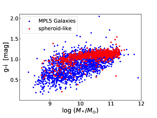
In our analysis we use the MaNGA MPL5 data, which includes a total of 2778 galaxies from the first two years of MaNGA survey operations, and is released in the SDSS fourteenth data release (SDSS DR14 Abolfathi et al., 2018). We adopt the morphology classification from Wang et al. (2018), in which the morphological type of each galaxy is classified into three broad classes: disk-like, spheroid-like and irregular, by visually inspecting its $r$-band image in the SDSS. Our analysis focuses on the spheroid-like class. After excluding galaxies with apparent problems in data reduction and/or spectral fitting, we obtain a sample of 894 galaxies. The spheroid-like object defined here is a stricter classification of ETG than in the widely-used Galaxy-Zoo classification (Willett et al., 2013). Some ETGs in Galaxy-Zoo classification have spiral-like features in their image, and thus are dropped from our sample (Wang et al., 2018). We have also compared our sample with the ETGs from a value-added catalogue of MaNGA galaxies presented in Fischer et al. (2019). Although the two samples have differences in identifying S0 galaxies, they are very similar in their mass and color distributions. Such differences are not expected to affect our main results. Fig. 1 shows the distributions of the MPL5 galaxies and of our sample galaxies in the $g-i$ colour versus $M_{*}$ plane, where both $M_{*}$ and $g-i$ are obtained from NSA. The total stellar masses of galaxies provided by NSA are derived from the fit to the SDSS five-band photometry with K-corrections (Blanton & Roweis, 2007), using the Bruzual & Charlot (2003) model and the Chabrier (2003) IMF.

Figure 1: Stellar mass-colour distribution of MPL5 galaxies. Galaxies visually identified as ‘spheroid-like’, which are used in our analysis, are shown in red dots, while the other two classes, disk-like and irregular, are shown by the blue dots. The $g-i$ color and the total stellar mass $M_{*}$ are adopted from NSA catalog.

2.3 Data reduction

The IFU spectra used in the paper are extracted using the MaNGA official data reduction pipeline (DRP, Law et al. 2016). DRP produces sky-subtracted, spectrophotometrically calibrated spectra, and combines individually dithered observations into three dimensional data cubes. Relative flux calibration for the MaNGA data is better than $5\%$ (Yan et al., 2016b). Additional information adopted in our analysis comes from the MaNGA Data Analysis Pipeline (DAP, Westfall et al., in preparation). This pipeline uses publicly available code, pPXF (Cappellari & Emsellem, 2004; Cappellari, 2017), to fit the stellar continuum and nebular emission lines of each spectrum, returning the kinematics of both components. We use their results for the stellar components, including the stellar velocity and velocity dispersion maps, as well as the elliptical polar radius of each spaxel from the galaxy center, normalized by the elliptical Petrosian effective radius from the NSA.

2.4 Stacking of spectra

In general, the flux variation caused by different IMFs is only at a few percent level (e.g. Conroy & van Dokkum, 2012a) due to the large mass-to-light ratio of dwarf stars (e.g. Maraston, 1998). Thus, to analyze the IMF variations generally requires spectral signal to noise ratio (SNR) of at least 100 Å^-1 (e.g. Ferreras et al., 2013), which is often achieved only by stacking spectra from a sample of galaxies, prohibiting such analyses for individual galaxies. The original DRP spectra, with typical $r$-band SNR of $4-8$ Å^-1 in the outer parts of galaxies, are obviously not sufficient for detailed analyses of IMF variations within individual galaxies. However, with the help of thousands of spectra in each IFU plate, one can obtain galaxy spectra with sufficiently high SNR by combining the spaxels of individual galaxies.

In this paper, we study two kinds of stacked spectra for different purposes. First, to study the global properties of individual galaxies and the variations of these properties from galaxy to galaxy, we co-add all the spaxels inside one effective radius ($R_{e}$, from NSA) of a galaxy into a single spectrum. Since the SNR is expected to increase by a factor of $N^{1/2}$, with $N$ being the number of spaxels, the stacked spectra of individual MaNGA galaxies can reach the SNR needed to study IMF effects. Unfortunately, spaxels from a single galaxy are still insufficient to reach the required SNR for a detailed investigation of the radial gradient of its IMF. To study potential radial variations in the IMF, therefore, requires a different kind of stacking. Here we first divide our sample into four subsets according to galaxy stellar mass, with $\log(M_{*}/M_{\odot})\in[8.0,10.0]$, $[10.0,10.5]$, $[10.5,11.0]$, and $[11.0,12.0]$, respectively. In each mass bin, the spaxels within $1R_{e}$ for individual galaxies are separated into 10 radial bins according to their normalized radii of elliptical annuli, using a bin size of $0.1R_{e}$. These radial bins from different galaxies are then combined accordingly to produce a final set of $4\times 10$ spectra to be used for the analyses of the radial dependence.

The binning procedure is as follows. Before performing the stacking, we take advantage of the high quality masks produced by the DRP and DAP to get rid of all the quantities that are problematic, such as low or no fibre coverage, and foreground star contamination. These masked individual pixels in the spectra from DRP, and the corresponding outputs of stellar velocity, $v$, and velocity dispersion, $\sigma_{*}$, from DAP are excluded. To do the stacking, we first convert the wavelengths of each spectrum to the rest-frame, using the redshift $z$ of each galaxy as given by NSA and the stellar velocity $v$ from the DAP. A cut at ${\rm SNR}=10$ is used to ensure the accuracy in the measurements of kinematics. The flux, inverse-variance and spectral resolution vectors from DRP are then interpolated to a common wavelength grid, uniformly sampled in the logarithmic space. For spaxels from the same galaxy, we calculate the direct mean of the flux at each wavelength point, which corresponds to a light-weighted average flux. For the stacking of radial bins of different galaxies, we first normalize the spectra in the wavelength window $4500-5500$ Å, which takes into account the flux variations among galaxies, and then calculate the inverse-variance weighted average of the flux at each wavelength point to maximize the SNR. The error vectors are then generated from the error propagation formula. For the velocity dispersion, we use the quadratic mean of the velocity dispersions measured from individual spectra as an initial estimate for the stack.

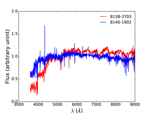
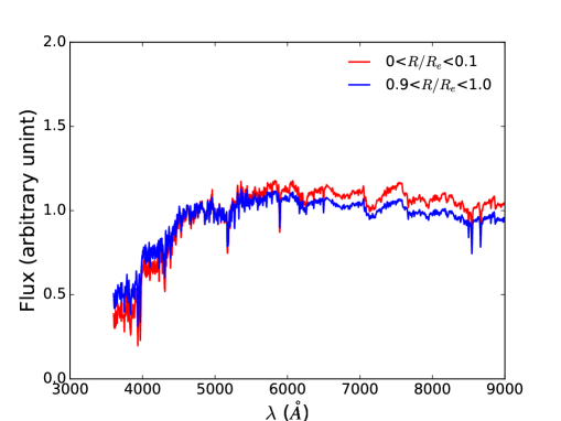
Examples of the spectra finally used in the paper are shown in Fig 2. As one can see, the SNR of the stacked spectra of individual galaxies within $1R_{e}$ varies from galaxy to galaxy. The typical SNR of the stacked spectra are around 200 pixel^-1, with wavelength dependence that peaks at around 6000 Å and drops towards both the red and blue ends. High mass galaxies typically have old red spectra, while lower mass galaxies have bluer spectra, with emission lines. For the radially stacked spectra of a sample of galaxies, the central regions are typically redder than the outer parts. The SNR is significantly enhanced in the stacked spectra, and is at least 500 pixel^-1 even for the outer bins. It should be noted, however, that some sky line residuals, especially in the near-IR wavelength range, can be seen in the spectra of individual galaxies, which may potentially bias our IMF inferences. However, these residual contaminants are greatly reduced in the stacked spectra, apparently because they are averaged out when the spectra of galaxies at different redshifts are corrected to the rest frame. To make full use of this crucial benefit, we obtain the average properties of a sample of galaxies from the stack spectra, rather than from the mean of the quantities derived from individual spectra.

Figure 2: Top panel: stacked spectra within $1R_{e}$ for two ETGs with NSA central velocity dispersion $\sigma_{*}$ equal to 230 km s^-1(red) and 74  km s^-1(blue), respectively. Bottom panel: radially binned spectra for the most massive sample (NSA $M_{*}>10^{11}{\rm M}_{\odot}$) in the central (red) and outer (blue) radial bins.

3 Analysis

Figure 3: Examples of IMF models used in our analysis, as labeled.

To infer properties of the IMF from galaxy spectra, one needs to compare stellar population models with the observed spectra, either by using some IMF-sensitive features or by fitting an entire spectrum. These two approaches are complementary. In general, the full spectrum contains more information, but it may be difficult to disentangle different factors that can affect the spectrum of a galaxy. In contrast, absorption features selected may be sensitive only to specific stellar populations, which may miss important information contained in the spectrum. In this paper, we adopt the approach based on full spectrum fitting, using an approach based on Bayesian statistics to infer the IMF and its co-variances with other properties.

3.1 The spectral synthesis model

The stellar population synthesis approach has long been adopted as the standard tool to interpret galaxy spectra (see Conroy, 2013, for details). In this approach, the time evolution of stars of different masses from the zero-age main sequence to their deaths is used to compute isochrones, which are the age-dependent distribution of stars in the Hertzsprung-Russell (HR) diagram. With the use of empirical and/or empirically-calibrated theoretical stellar libraries to assign a spectrum to each point in the HR diagram, the integrated light from a coeval set of stars (referred to as a simple stellar population, SSP) can be obtained by summing up the spectra along an isochrone, weighted by the number of stars at a given stellar mass, as specified by the IMF of stars. Finally, for a composite stellar population (CSP), such as a galaxy, the spectrum can be obtained through the convolution of the time-dependent SSPs with the star formation history (SFH) of the galaxy, together with a prescription for dust attenuation. In what follows we describe briefly the SSP models we use.

3.1.1 Models of  SSP

There are several popular SSP models, e.g. BC03 (Bruzual & Charlot, 2003), M05 (Maraston, 2005), CvD12 (Conroy & van Dokkum, 2012a) and E-MILES (Vazdekis et al., 2016), that are based on different stellar templates and isochrones. Each of these models has its own merits and shortcomings. Since we are interested in the inference of the IMF, whose effects are the strongest in the near infrared (NIR) (Ferreras et al., 2013), we need to select SSP models that can provide consistent predictions all the way to the NIR. This kind of SSP models are currently rare and calibration may be a problem in many of them. In this paper, we select a set of state-of-the-art E-MILES models as our SSP templates.

The E-MILES models are the latest version of the MILES models originally presented in Vazdekis et al. (2010). They are constructed using the MILES (Sánchez-Blázquez et al., 2006), CaT (Cenarro et al., 2001) and Indo-U.S. (Valdes et al., 2004) empirical stellar libraries, extended to the infrared with the use of the IRTF stellar library (Cushing et al., 2005; Rayner et al., 2009). Self-consistent E-MILES SSP spectra are computed to cover the wavelength range from 1680.2 Å to $5{\rm\mu m}$, with a moderately high spectral resolution. In particular, these SSPs can reach a high resolution of 2.51 Å (FWHM) over the range from 3540 Å to 8950 Å, which is of special interest in our analysis. Since the wavelength range of the original MaNGA data is $3600-10300$ Å, most of the spectra will fall within this range after corrected to the restframe. We thus limit our analysis of the stacked spectra only to this wavelength range.

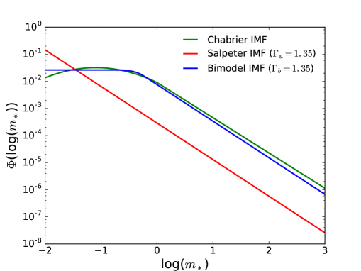
The E-MILES SSPs are computed for several IMFs, including the widely used Salpeter (Salpeter, 1955), Kroupa (Kroupa, 2001) and Chabrier (Chabrier, 2003) IMFs, and two parameterized forms, unimodel and bimodel (Vazdekis et al., 1996), both including a lower and an upper mass-cutoff set at $0.1M_{\odot}$ and $100M_{\odot}$, respectively. The unimodel IMF is a simple power law over the entire mass range, characterized by the power law slope, $\Gamma_{u}$:

$$\Phi(m)\propto m^{-(\Gamma_{u}+1)}~{}~{}~{}~{}(\text{unimodel})\,.$$ (1)

Thus, the Salpeter IMF is a special case of this kind with $\Gamma_{u}=1.35$. In contrast, the bimodel IMF is the same as the unimodel IMF at $M_{*}>0.6M_{\odot}$, characterized by a similar power law slope $\Gamma_{b}$, but turns to a flat distribution at the lower mass end:

$$\Phi(m)\propto\left\{\begin{array}[]{lr}(m/0.6)^{-(\Gamma_{b}+1)}&\text{(for $m>0.6$)}\\ p(m)&\text{(for $0.2\leq m\leq 0.6$)}\\ 1&\text{(for $m<0.2$)}\end{array}~{}~{}~{}(\text{bimodel})\,.\right.$$ (2)

where $p(m)$ is a third degree spline between the low- and high-mass ends of the IMF. The relatively low fraction of low-mass stars in this IMF is in agreement with that inferred from the Milky Way. In fact, a bimodel IMF with $\Gamma_{b}=1.3$ is a good approximation to the Kroupa IMF. Some examples of these IMFs are shown in Fig 3. In what follows, we will compare the Milky-way like and bottom-heavy IMFs in our model selection analysis, while using unimodel and bimodel to investigate the shape of the IMF.

3.1.2 Star formation history and dust extinction

The star formation history (SFH) of a galaxy can in principle be very complex, and it is difficult to come up with a universal model that can describe the SFHs of every individual galaxies. Furthermore, the SFH may also vary across a galaxy, which makes it even more difficult to model the spectra in an IFU survey such as MaNGA. Currently there are two ways to model the SFH. The first one, a non-parametric approach, is to divide the SFH into a number of time bins and to consider all stars that form in each bin as an SSP. The SFH is then specified by the average star formation rates in individual time bins. This approach avoids the need for a specific model for the SFH, and has been adopted in a number of spectral fitting codes, such as STARLIGHT (Cid Fernandes et al., 2005) and pPXF (Cappellari & Emsellem, 2004). However, the problem with this approach is that the total number of SSPs with non-zero weights limits the time resolution, and the interpretation of the results are not straightforward. The second way is to assume a functional form for SFH, which is specified by a small number of parameters. The advantage here is that the SFH has an infinite time resolution, and the number of free parameters is usually small so that the model can be well constrained. The disadvantage is, of course, that the functional form adopted may not describe the real SFHs properly, which may lead to biased inferences.

Since our main focus here is on early-type galaxies, which often have relatively simple SFH, we choose the latter approach. The SFH model considered here is represented by the Gamma function:

$$\Psi(t)=\frac{1}{\tau\gamma(\alpha,t_{0}/\tau)}\left({t_{0}-t\over\tau}\right)^{\alpha-1}e^{-(t_{0}-t)/\tau}\,,$$ (3)

where $t_{0}-t$ is the look-back time, $\gamma(\alpha,t_{0}/\tau)\equiv\int_{0}^{t_{0}/\tau}x^{\alpha-1}e^{-x}\,dx$ is used to normalize the SFH over the age of the universe $t_{0}$, which is assumed to be 14 Gyr. This is a two-parameter model, with the parameter $\tau$ characterizing the time scale for the onset of star formation, and the parameter $\alpha$ adopted to make the SFH flexible. This SFH ensures that the star formation rate goes to zero at early time, peaks at intermediate time, and then decays exponentially at late time, as is seen for ETGs in numerical simulations and semi-analytic models (Lu et al., 2015).

The dust attenuation is known to have degeneracy with the age and metallicities of stars in spectral fitting. Therefore, dust extinction has to be properly taken into account in order to derive the properties of galaxies from their observed spectra. In general, one assumes an attenuation curve and treats the dust extinction as an additional model parameter. The widely used Calzetti Law (Calzetti et al., 2000) describes the dust content and opacity of star-forming galaxies, while the two component dust model by Charlot & Fall (2000) accounts for the differences between nebular and stellar continuum extinction. The dust properties of the ETGs concerned here are believed to be simple, and so a single optical depth parameter describing the attenuation of the entire stellar population in a galaxy may be sufficient.

We note that some low-mass ETGs may contain complex stellar populations and complex dust components, and our simple models for the SFH and dust extinction may not work properly. For those galaxies, a more complex model or, alternatively, a high order polynomials to deal with the continuum mismatch as done in pPXF, may be needed to get better fits to their spectra. However, these additional components often reduce the fitting efficiency and have no straightforward interpretations. Throughout this paper, we will stick to the simple model, but will examine the reliability of our results against our model assumptions.

3.1.3 Stellar kinematics

The intrinsic motion of stars in a galaxy induces Doppler shifts in their spectra, and so can change the synthesized spectrum. Detailed modeling of the stellar kinematics often uses a Gaussian-Hermite decomposition of the line of sight velocity distribution. In practice, however, it is usually sufficient to use the second moment of the velocity distribution, i.e. the velocity dispersion $\sigma$, to model the effect. Furthermore, as each of our stacked spectrum is the sum of a relatively large number of pixels, a Gaussian broadening is expected from the central limit theorem. An estimate of the velocity dispersion in the stack can thus be obtained by the accumulative effect of a set of Gaussian functions characterized by the velocity dispersion of individual spectra. As described in §2.4, the velocity dispersion, $\sigma$, of a stacked spectrum is estimated from the quadratic mean of the velocity dispersion of individual spectra in the stack, and this estimate is denoted by $\sigma_{dap}$. The profile of $\sigma_{dap}$ exhibits a well-known negative gradient for early-type galaxies (e.g. Emsellem et al., 2004). We note that this estimate of the central (the $r<0.1R_{e}$ bin) velocity dispersion is systematically higher than that obtained from NSA due to the difference in the aperture size, but the difference is typically smaller than 10%. In our modeling, we use $\sigma_{dap}$ to characterize the motion of stars. When discussing the global properties, however, we use the NSA dispersion, quoted as $\sigma_{*}$, for the convenience in comparing with the other results.

However, the velocity dispersion estimated this way does not account for the exact broadening of the stacked spectra. As the DAP measurements of stellar velocities are used to correct the spectra to the rest frame, the measurement errors can cause shifts in wavelength, leading to an additional broadening in the stacked spectra. This effect is particularly significant in the outer regions of galaxies where the SNR is relative low (Cappellari, 2017; Parikh et al., 2018). In order to obtain a more accurate estimate of the broadening for each stacked spectrum, we perform spectral fitting with the software pPXF in the range $3400-7400$ Å (equivalent to MaNGA DAP) using a set of E-MILES SSPs. pPXF can be used to perform full spectra analysis, but here we use it only to estimate the broadening of a spectrum. The use of template SSPs with different IMFs only affects the $\sigma$ measurement at $\lesssim 1\,{\rm km/s}$ level (e.g. Ferreras et al. 2013), and so we fix the IMF to be Salpeter in this part of our analysis. The effective velocity dispersion, obtained this way from a stacked spectrum and referred to as $\sigma_{ppxf}$, is then used in our fitting of the stacked spectrum over the whole wavelength range to derive other quantities. Because of the artificial broadening described above, $\sigma_{ppxf}$ are systematically larger than $\sigma_{dap}$ except in the central region.

3.2 The Bayesian approach

Figure 4: Left: An example of fitting a stacked spectrum. The blue line is the input spectrum, while the red line is the best-fit model spectrum obtained from the posterior distribution of model parameters. The green line shows the residual, with grey shaded regions denoting the noise level of the data. The vertical shaded region indicates the part of the spectrum that is masked out in the fitting due to affects from residual telluric absorption and flux calibration difficulties. Right: The corresponding best-fit star formation history (normalized to $1{\rm M_{\odot}}$) of the galaxy inferred from the posterior distribution.

Figure 5: Posterior probability distribution of the model parameters listed Table 1 for the spectrum shown in Fig. 4. The diagonal panels show the marginal distributions of $\Gamma_{u}$, $\log(Z/Z_{odot})$, $\tau$, and $\alpha,\tau_{v}$, respectively. The off-diagonal panels show the joint distributions of parameter pairs.

The spectral fitting code used here is called the Bayesian Inference of Galaxy Spectra (BIGS), which can perform full Bayesian analysis to infer physical properties of galaxies from their spectra. The idea of Bayesian approach is to provide a statistically rigorous way to estimate the parameters, $\theta$, that specify a model (or hypothesis), $H$, given the constraining data $D$. Bayes’ theorem states that the probability distribution of $\theta$ given $D$ can be written as

$$P(\theta|D,H)=\frac{P(D|H,\theta)P(\theta|H)}{E}\,.$$ (4)

Here $P(\theta|D,H)$ is the posterior probability distribution of the model parameters. $P(D|H,\theta)$ is the likelihood function, which describes the probability distribution of the data for the model $H$ with parameters $\theta$. $P(\theta|H)\equiv\pi(\theta)$ represents our prior knowledge about the model parameters. The normalization,

$$E\equiv P(D|H)=\int P(D|H,\theta)P(\theta|H)d\theta\,,$$ (5)

is the Bayesian evidence which describes how well the hypothesis $H$ can accommodate the data, which is of special importance in Bayesian model selection. In the Bayesian context, the evidence ratio measures the posterior probability ratio between two competing model families. Suppose we have two models, $H_{1}$ and $H_{2}$, then

$$\frac{Pr(H_{1}|D)}{Pr(H_{1}|D)}=\frac{Pr(D|H_{1})Pr(H_{1})}{Pr(D|H_{2})Pr(H_{2})}=\frac{E_{1}}{E_{2}}\frac{Pr(H_{1})}{Pr(H_{2})}\,,$$ (6)

where $Pr(H_{1})/Pr(H_{2})$ is the prior probability ratio for the two models. If there is no a priori reason for preferring one model over the other, we can set $Pr(H_{1})/Pr(H_{2})=1$, so that the ratio of the posterior probabilities of the two models given the data $D$ is equal to their evidence ratio.

For the problem concerned here, BIGS works as follows. To begin with, a data spectrum, and a set of model spectra convolved with a Gaussian to account for instrumental resolution and velocity dispersion of stars, are provided to BIGS. BIGS then uses the Bayesian sampler, MULTINEST (Feroz et al., 2009; Feroz et al., 2013), to produce a set of proposal parameter vectors for the spectral synthesis model, including parameters describing SFH, IMF, metallicity and dust attenuation. A model spectrum is generated from these parameters, and is used to calculate the likelihood by comparing the model prediction with the data (see eq.7 below for an example). This likelihood is then returned to the MULTINEST sampler, which makes a decision to accept or reject the proposal on the basis of the posterior probability and generates a new proposal for the model. This MULTINEST-model loop continues until convergence is achieved. The converged states, which sample the full probability distribution of the model parameters (the posterior distribution), are stored and to be used to derive statistical inferences of the model.

3.3 The fitting procedure

To make quantitative statements about the IMF of a galaxy, we fit E-MILES templates to the stacked spectra, using the procedure described below. Our extensive test shows that almost all SSP templates have difficulties to fit the observed continua in the wavelength range 6800-8100 Å. This mismatch between model and data results in a flux difference at several percent level and can potentially bias our inferences about IMF. It is commonly found in several studies and can relate to issues in flux calibration difficulties in the templates (e.g. Conroy & van Dokkum 2012a), residual telluric absorption (e.g. Vaughan et al. 2018a), or even the flux calibration of the data itself. The introduction of a high order polynomial, as in MaNGA DAP, or splitting the wavelength range to be fitted into several segments (e.g. Vaughan et al. 2018a) can relieve the problem, but significant residuals still present. We choose to mask out the entire problematic region, between 6800 and 8100 Å, and only to use the rest of the spectrum in our fitting. Note that spectral regions that contain most of the IMF-sensitive features, such as TiO1 at 5970 Å, TiO2 at 6240 Å, NaI doublet at 8190 Å, and the calcium triplet CaT at 8400-8600 Å, are used in our fitting, although constraints on the IMF may also come from other spectral properties.

As described in §3.1.3, to take into account effects of stellar kinematics, we first fit a stacked spectrum using pPXF to extract an effective velocity dispersion, $\sigma_{\rm ppxf}$, which contains all factors that contribute to spectral broadening, such as errors in the measurements of stellar velocities, intrinsic dispersion, and instrumental resolution. Template spectra from the E-MILES library are convolved with a Gaussian kernel according to this effective velocity dispersion. We have made tests by using the NSA dispersion instead of $\sigma_{\rm ppxf}$, and found that the measured stellar population parameters remain stable, presumably because our measurements are not sensitive to the details of spectral broadening. Note that, in this step of spectrum fitting, spectra with apparent emission lines are identified, and are masked out in subsequent analyses. However, since emission lines are not common and generally quite weak for galaxies in our sample, excluding these lines does not make a significant difference.

After the pre-processing described above, both the model and data spectra are first normalized in the wavelength window $4500-5500$ Å, so as to match the stacking procedure described in §2.4, and then sent to BIGS. We have made tests by using normalization in different spectral regions, and found that our results are not affected. BIGS runs the fitting loop as described in §3.2, with a flat prior and a $\chi^{2}$-like likelihood function, $L(\theta)\equiv P(D|H,\theta)$, which can be written as

$$\ln{L(\theta)}\propto-\sum_{i,j=1}^{N}\left(f_{\theta,i}-f_{D,i}\right)\left({\cal M}^{-1}\right)_{ij}\left(f_{\theta,j}-f_{D,j}\right)\,$$ (7)

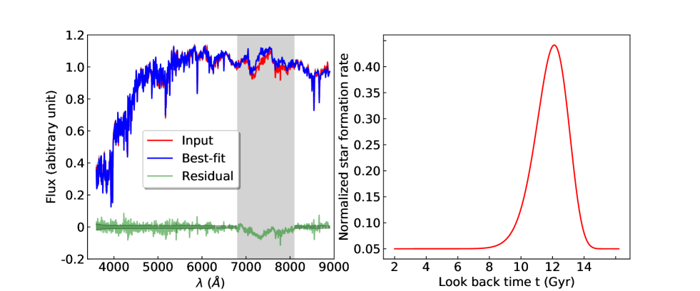
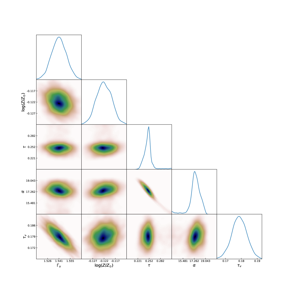
where $N$ is the total number of wavelength bins, $f_{\theta}$ and $f_{D}$ are the flux predicted from the parameter set $\theta$ and that of the data spectrum, respectively, and ${\cal M}_{ij}\equiv\langle\delta f_{D,i}\delta f_{D,j}\rangle$ is the covariance matrix of the data. Convergence is assumed to be achieved when changes in the Bayesian evidence $\Delta\ln{E}<0.5$ in a new loop. After convergence, the sample of the posterior of the model parameters and the overall evidence of the model are stored for subsequent analyses. We list all the fitting parameters in Table 1, together with their prior distributions (assumed to be flat). An example of the fitting is shown in Fig. 4 together with the inferred SFH. The posterior distributions of the model parameters are shown in Fig. 5.

Table 1: Priors of model parameters used to fit galaxy spectra

Parameter	description	Prior range
$\Gamma_{u}$; $\Gamma_{b}$	IMF slopes	$[0.3,3.5]$
$\log(Z/Z_{\odot})$	metallicity	$[-2.3,0.2]$
$\tau$	SFH parameter in Eq. (3)	$[0.0,10.0]$
$\alpha$	SFH parameter in Eq. (3)	$[0.0,20.0]$
$\tau_{v}$	dust optical depth at 5500 Å	$[0.0,2.0]$

4 Inferences of the variations of the initial mass function

4.1 IMF model selection

Figure 6: The evidence ratio between Chabrier and Salpeter IMF as a function of galaxy velocity dispersion. Each red dot stands for the result of a MaNGA ETG. Blue stars are the median values in five $\sigma_{*}$ bins and are linked by a blue line. Error bars are obtained from the jackknife resampling method.

Figure 7: The evidence ratio between bimodel and unimodel as a function of galaxy velocity dispersion. Each red dot stands for the result of a MaNGA ETG. Blue stars are the medians in the five $\sigma_{*}$ bins and linked by a blue line. Error bars are obtained from the jackknife resampling method.

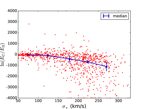
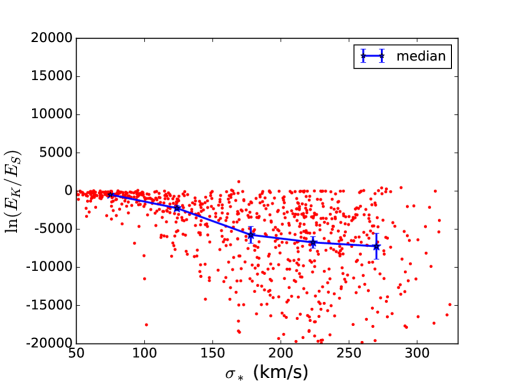
The Bayesian approach described above can provide an overall evidence for any given model family of the IMF. As described in §3.2, the Bayesian evidence ratio is a measure of the posterior probability ratio between two competing model families and, therefore, can be used to distinguish different models. Thus, before investigating the variations of the IMF with galaxy properties, it is useful to use Bayesian evidence to examine whether the observational data prefers one form of the IMF among all the forms described above. To this end, we first fit the stacked spectra (each being a stack of pixels within the effective radius of a galaxy) of individual galaxies with the two selected set of E-MILES SSPs assuming the two widely-used IMFs, the Chabrier IMF and the Salpeter IMF, while keeping all other parts of the model intact. We then use the evidence ratio between the two fits to gauge the preference of the data between the two models. Fig. 6 shows $\ln(E_{\rm C}/E_{\rm S})$ versus the NSA velocity dispersion, $\sigma_{*}$, obtained from spatially unresolved analysis, where $E_{\rm C}$ and $E_{\rm S}$ stand for the Bayesian evidences of the Chabrier and Salpeter IMF models, respectively. The median values in five $\sigma_{*}$ bins are plotted as blue stars to demonstrate the average trends. To estimate the statistical error, we randomly divide our sample into 20 sub-samples, and calculate the median in 20 different jackknife copies by eliminating one of the 20 sub-samples. The statistical error is then derived from the 20 jackknife medians, which are shown in Fig. 6 as error bars. There is a clear trend in the evidence ratio with the velocity dispersion: the evidence ratio decreases with increasing $\sigma_{*}$. Overall, there is a preference to the Salpeter IMF by galaxies with $\sigma_{*}>150\,{\rm km/s}$, while such a preference is absent for galaxies with lower $\sigma_{*}$. Note that very few galaxies of high $\sigma_{*}$ prefer Chabrier IMF over Salpeter IMF, although many of them appear indifferent to both.

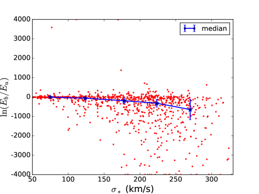
Next we compare the two model families, unimodel and bimodel. Fig. 7 shows $\ln(E_{\rm b}/E_{\rm u})$ versus $\sigma_{*}$, where $E_{\rm b}$ and $E_{\rm u}$ stand for the Bayesian evidences of the bimodel and unimodel IMFs, respectively. Interestingly, although results are generally concentrated around zero, there is a weak trend showing a decreasing evidence ratio with increasing $\sigma_{*}$, i.e. a preference to the unimodel IMF. This result indicates that the IMF of early type galaxies is more likely to be a power law all the way to the low mass end, instead of becoming flat as does the Galactic IMF, such as the Chabrier IMF (Chabrier, 2003) and the Kroupa IMF (Kroupa, 2001). This result is, however, in conflict with some of the results that take into account dynamical constraints (e.g. La Barbera et al., 2013; Lyubenova et al., 2016), which indicates that the IMF parameterization adopted here may not be a good model for these galaxies (see discussions in §5.1).

Unfortunately, it is not straightforward to have a quantitative decision about the IMF type. A naive classification, such as identifying all galaxies with $\ln(E_{C}/E_{S})>0$ as the ones that prefer the Chabrier IMF, may not be unreliable, because the scatter presented in Fig. 6 is large and it is unclear whether it is produced by intrinsic variations or by noise. In what follows, we will present results mainly based on unimodel, although we sometimes also show bimodel results for comparison.

4.2 Dependence on galaxy velocity dispersion

Figure 8: The best-fit slope of the unimodel (left) and bimodel (right) IMF for MaNGA ETGs plotted against central velocity dispersion. In each panel, small red dots stand for the results of individual MaNGA ETGs. The Pearson correlation coefficient, $r$, is shown on the top of each plot to quantify the correlation between the IMF slope and the velocity dispersion. Big thick dots are the results derived from the stacked spectra in five $\sigma_{*}$ bins, while the red line is a fit to these points. The errorbars are obtained from 20 jackknife samples. The grey dash line denotes the slope of the Salpeter IMF. Blue and green lines are predictions by assuming the IMF variation is is driven by metallicity and age (see §4.5), respectively. Results from Ferreras et al. (2013) and La Barbera et al. (2013) are shown as yellow and black lines, respectively.

Figure 9: Unimodel IMF slope as a function of metallicity in different $\sigma_{*}$ bins. The red, green, blue dots stand for galaxies in three $\sigma_{*}$ bins, as indicated. The Pearson correlation coefficient, $r$, between the IMF slope and metallicity is shown on the top of the panel. The big symbols connected thick lines are the median values in each $\sigma_{*}$ bin. Error-bars are obtained from the jackknife method. The black dash line shows the result from Martín-Navarro et al. (2015b).

Figure 10: Unimodel IMF slope as a function of $\sigma_{*}$ in different metallicity bins. The red, green, and blue dots stand for galaxies in three metallicity bins, as indicated. The Pearson correlation coefficient, $r$, between $\Gamma_{u}$ and $\sigma_{*}$ is shown on the top of the panel. The big symbols connected by thick lines are median values in each $Z$ bin. Error-bars are obtained from the jackknife method.

Figure 11: Top panels: optical images of six example galaxies, with MaNGA plate-ifu shown on top of each image. Bottom panels: joined posterior distribution estimated from the fitting results with standard setting. The first and second rows show the covariance between the IMF slope, $\Gamma_{u}$, with the stellar metallicity, $Z$, and mean stellar age, $A$, respectively. The last row shows the covariance between $A$ and metallicity $Z$. Red dash lines in each row show the degeneracy line inferred from the median value of the whole sample. The slopes of these lines are $\Delta\Gamma_{u}/\Delta\log(Z)=-0.34$, $\Delta\Gamma_{u}/\Delta\log(A)=0.22$, and $\Delta\log(A)/\Delta\log{Z}=-1.42$, respectively.

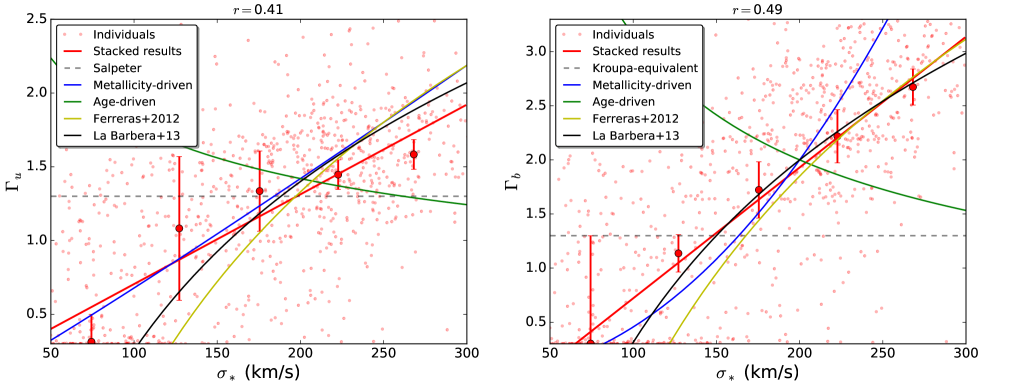
We fit the MaNGA spectra (stacked within $1R_{e}$) of individual galaxies with both unimodel and bimodel described above. The Gamma model for the SFH (referred to as $\Gamma$-SFH) and a one-component dust model are assumed, together with a metallicity parameter. The fits to the spectra are in general quite good, with residual at around the $3\%$ level over a large range of wavelength. The results for unimodel and bimodel are shown in Figs. 8. The best-fit slopes of the IMF are generated from the posterior distribution through marginalizing over the rest of model parameters. The velocity dispersion used in the plots is the NSA velocity dispersion, $\sigma_{*}$, adopted for the convenience to compare with previous studies. The small red dots are the results for individual galaxies, while the bigger blue squares are the mean results in five $\sigma_{*}$ bins, obtained by fitting the total composite spectrum in each of the $\sigma_{*}$ bins. We again make use of the jackknife resampling method to estimate the statistical error. To this end, we randomly divide our sample into 20 sub-samples, and generate 20 different jackknife copies of the stacked spectra by eliminating one of the 20 sub-samples in each stack. The same fitting algorithm is then applied to each of the 20 jackknife copies to obtain the corresponding IMF slope. The variance of the IMF slope values estimated from the jackknife copies are shown in the in Figs. 8 as the error bars. The Pearson correlation coefficient $r$ between the pair of plotted quantities is shown on the top of each panels to quantify the strength of the correlation.

As one can see, the IMF slopes in both unimodel and bimodel increase with the velocity dispersion of the ETGs. This indicates clearly that the IMF is non-universal, but changes systematically in that the contribution of low-mass stars is higher in more massive galaxies. In the unimodel, the IMF slope can even be steeper than the Salpeter IMF for ETGs with the highest $\sigma_{*}$, suggesting that the IMF of these galaxies is significantly bottom-heavy. If the IMF is forced to have a turnover at $m<0.6$, as in bimodel, the majority of the galaxies at $\sigma_{*}>200\,{\rm km/s}$ require $\Gamma_{b}>1.35$, again indicating the preference to a bottom-heavy IMF. Note that $\Gamma_{b}$ has stronger dependence on $\sigma_{*}$ than $\Gamma_{u}$, because the suppression of stars at $m<0.6$ in bimodel has to be compensated by a steeper slope so as to produce sufficient amounts of low-mass stars to match the spectra of high $\sigma_{*}$ galaxies. As shown in the plot, our results are in good agreement with those of Ferreras et al. (2013) and La Barbera et al. (2013), which is expected as we are using similar stellar population models although different fitting approaches.

4.3 Dependence on metallicity

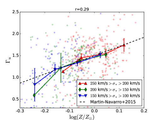
The small points in Fig. 9 show the IMF slope, $\Gamma_{u}$, against galaxy metallicity for individual galaxies. Here the metallicities are obtained directly from our fitting to individual spectra and marginalizing over the posterior distributions. We focus on galaxies with metallicities in the range $-0.3<\log(Z/Z_{\odot})<0.2$ in which the majority of our sample galaxies are contained. As one can see, there is a strong correlation between the IMF shape with metallicity. This correlation may not be surprising, as galaxy metalicities are known to be correlated with the depth of its gravitational well, as represented by its velocity dispersion (e.g. Gallazzi et al., 2005). Our result is in good agreement with that of Martín-Navarro et al. (2015b), who found that the correlation of the IMF shape with metallicity is the strongest among those with a number of other galaxy properties, including galaxy velocity dispersion. However, as can be seen from the correlation coefficients, the IMF slope-metallicity relation is not as tight as the IMF slope-$\sigma_{*}$ relation. This is likely due to age-metallicity degeneracy, which has not been taken into account here but will be discussed in more detail in §4.5.

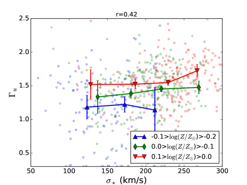
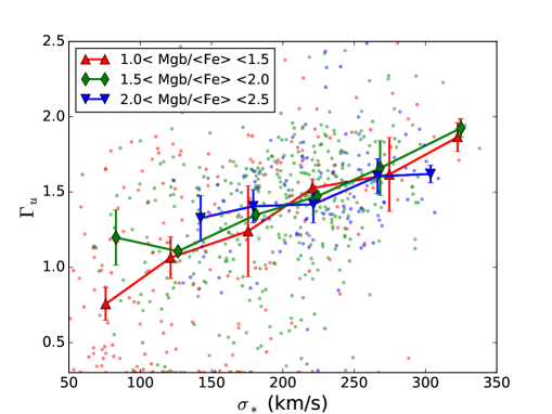
The large sample used here allows us to analyze the correlations of the IMF shape with velocity dispersion and metallicity independently, so that we can investigate whether the systematic change of the IMF slope is driven by velocity dispersion or by metallicity. The solid lines in Fig. 9 show the average $\Gamma_{u}$ - metallicity relations in three $\sigma_{*}$ bins. As one can see, the dependence on metallicty is very similar for galaxies of different velocity dispersions, indicating that it is the matallicity that produces the $\sigma_{*}$ dependence of the IMF slope. As comparison, we show in Fig. 10 the IMF slope as a function of galaxy velocity dispersion for individual galaxies separated into different metallicity bins. The dependence of the IMF slope on $\sigma_{*}$ is significantly weakened for galaxies of similar metallicities, suggesting again that the dependence on $\sigma_{*}$ is metallicity driven.

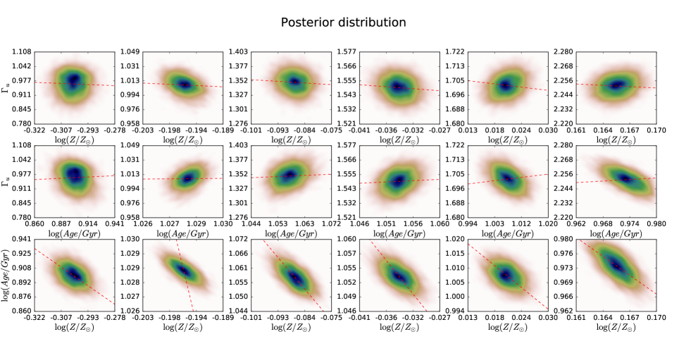
Since both the IMF slope and metallicity are model parameters in our spectrum fitting, it is important to check if the dependence of $\Gamma_{u}$ on $Z$ is produced by the degeneracy of these two parameters in the model. Our Bayesian approach allows us to examine such degeneracy for individual galaxies. In Fig. 11 we show the posterior distributions obtained from the MULTINEST sampling for six representative galaxies with different stellar masses, metallicities, and spectral signal-to-noise ratios. As one can see from the first row in the lower part of the figure, the statistical inference errors in both $\Gamma_{u}$ and $Z$ are much smaller than the ranges over which the correlation between $\Gamma_{u}$ and $Z$ is observed, indicating that the model parameters for individual galaxies are stringently constrained by their spectra. In particular, the median degeneracy relation obtained from the total sample, which has a slope $\Delta\Gamma_{u}/\Delta\log(Z)=-0.34$, as represented by the red dashed lines, is quite weak, indicating that the dependence of the IMF slope on $Z$ is not produced by the degeneracy of the two parameters in our spectrum fitting.

4.4 Dependence on stellar age and dust extinction

Figure 12: Unimodel IMF slope as a function of light weighted age. The red, green, and blue dots stand for galaxies in three metallicity bins, as indicated. The Pearson correlation coefficient $r$ between $\Gamma_{u}$ and age is shown on the top of the plot. The big symbols connected by thick lines are median values in each metallicity bin. Error bars are based 20 jackknife samples.

Figure 13: Unimodel (left) and bimodel (right) IMF slope as a function of $D\equiv AZ^{-1.42}$, where the age, $A$, is in units of Gyr and metallicity, $Z$, in units of solar metallicity. In each panel, the red, green, and blue dots are for galaxies in three age bins, as indicated.The Pearson correlation coefficient, $r$, between the quantities plotted, is shown on the top of each plot. The big symbols connected by thick lines are median values in each age bin. Error bars are based on 20 jackknife samples. The black straight lines show the fits to all the data points, and are $\Gamma_{u}\propto D^{-1.37}$ and $\Gamma_{b}\propto D^{-2.73}$, respectively.

From the constrained star formation history of a galaxy, we can also estimate a light-weighted average of stellar ages, $A$, to represent the characteristic age of the galaxy. The light-weighted ages are estimated as follows. With each given pair of $\tau$ and $\alpha$ values, Eq. (3) gives the normalized star formation rate as a function of time. Thus, the total mass of stars that form in a time interval at $t_{i}$ can be written as $\Delta M_{i}={\rm SFR}(t_{i})\Delta t_{i}$. Since the fluxes of SSPs provided by stellar population models in BIGS are normalized to $1M_{\odot}$ (Vazdekis et al., 2016), we assign $\Delta M_{i}$ to the SSP of the corresponding age and calculate a final spectrum as the sum of the fluxes from these SFR-weighted SSPs. In contrast, in traditional algorithms based on discrete SSPs, SSP fluxes from stellar population models are normalized at a specific wavelength $\lambda_{0}$. Light fractions are then assigned to such normalized SSP and the final spectrum is then calculated from the sum of the fluxes from these light-weighted SSPs (Cid Fernandes et al., 2005). To calculate a similar light-weighted age, we calculate the light fraction of the SSP that forms in the $i$th time interval, $x_{i}$, from the stellar mass of this SSP, $\Delta M_{i}$, using $x_{i}=\Delta M_{i}f_{i}(\lambda_{0})$, where $f_{i}(\lambda_{0})$ is the flux of the model SSP at the wavelength $\lambda_{0}$. The light-weighted ages are then obtained as

$$\langle A\rangle={\sum{x_{i}A_{i}}\over\sum{x_{i}}},$$ (8)

where $A_{i}$ is the age for the SSP that forms in the $i$th time interval.

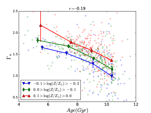
The small points in Fig. 12 show the IMF slope, $\Gamma_{u}$, as a function of galaxy age, $A$, for individual galaxies, while the big symbols connected by solid lines are the median relations for galaxies in different metallicity bins. The IMF shape appears to decrease with stellar age in all metallicity bins, indicating that the IMF slope may also depend stellar age, although the global correlation is quite weak, as indicated by the correlation coefficient. This result is similar to the anti-correlation between IMF slope and stellar age found in Martín-Navarro et al. (2015b) from CALIFA galaxies. The posterior distribution between the IMF slope and stellar age for the six representative galaxies are shown in the second row of the lower part of Fig. 11. The dashed red lines, which have a slope $\Delta\Gamma_{u}/\Delta\log(A)=0.22$, show the madian degeneracy line between $\Gamma_{u}$ and $A$ obtained from the total sample. The small, positive slope indicates that the dependence of $\Gamma_{u}$ on $A$ shown in Fig. 12 is not produced by the degeneracy. However, since the stellar age and metallicity are degenerate in spectrum fitting, it is important to check if the age-dependence of the IMF slope is independent of the metallicity-dependence. To this end, we show in the last row of Fig. 11 the posterior joint distribution of $A$ and $Z$ for the representative galaxies. For reference, we plot a dash line in each panel to show the degeneracy line, $AZ^{\beta}={\rm constant}$, where $\beta=1.42$, as is obtained by the median $A$-$Z$ degeneracy relation of individual galaxies. Note that the $\beta$ value obtained here is close to its canonical value, $1.5$, as obtained by Worthey (1994). There are variations in the degeneracy of $A$ and $Z$ from galaxy to galaxy, but the trend that $A$ varies inversely with $Z$ is the same for almost all galaxies. Because of this age-metallicity degeneracy, it is difficult to separate the age and metallicity effects on IMF, unless the age and metallicity can be determined independently. We will come back to this in §4.5.

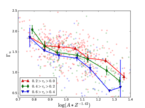
In our spectral fitting, dust extinction is modeled by a given extinction curve, and specified by an optical depth parameter. The dust optical depths obtained for individual galaxies from our fitting range from 0.0 to 0.6, indicating that dust extinction is quite small, as is expected for the ETGs concerned here. Since the dust absorption is stronger at shorter wavelengths, dust extinction makes a galaxy look redder, or older in its continuum shape. Degeneracy between the dust optical depth and the stellar age (or metallicity) is thus expected in the spectral fitting. We examine the influence of dust in the $\Gamma_{u}$-$D$ relation by separating galaxies into three specific optical depth bins, as shown in Fig 14. The figure shows that galaxies with higher dust optical depth have slightly lower $\Gamma_{u}$. This is expected from the degeneracy between the optical depth and age: an overestimate of dust extinction lead to an underestimate of stellar age (smaller $D$). The $\Gamma_{u}$-$D$ correlation would then shift to the left. A possible way to take into account this degeneracy is to use a combination of $A$, $Z$ and $\tau_{v}$ that is perpendicular to the degeneracy plane in the $(A,Z,\tau_{v})$ space. However, current data is too poor to establish such a degeneracy plane. Since the dust extinction is relatively small in our galaxies, and its influence on the $\Gamma_{u}$-$D$ relation is only modest, as shown in Fig 14, we will not discuss the dust effect any further.

4.5 The origin of IMF variation

Figure 14: Unimodel IMF slope as a function of $D\equiv AZ^{-1.42}$, where the age, $A$, is in units of Gyr and metallicity, $Z$, in units of solar metallicity. The red, green, blue dots stand for galaxies in three bins of the dust optical depth parameter, as indicated. The big symbols connected by thick lines are median values in each $\tau_{v}$ bin. Error bars are based 20 jackknife samples.

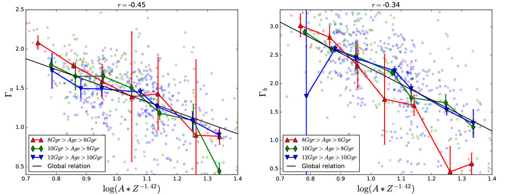
In order to see the effect of the age-metallicity degeneracy described above, we plot $\Gamma_{u}$ and $\Gamma_{b}$ versus $D\equiv AZ^{-\beta}$ in Fig. 13. Note that the line of a constant $D$ is perpendicular to the degeneracy line in the $\log(A)$ - $\log(Z)$ space, so that the effects of the age-metallicity degeneracy are expected to be reduced or eliminated along $D$, if the age-metallicity degeneracy were accurately described by the mean relation we use.As one can see from Fig.  13, the scatter in $\Gamma_{u}$ is indeed reduced relative to that in the $\Gamma_{u}$ - $A$ and $\Gamma_{u}$ - $Z$ relations. This is also true for the results of $\Gamma_{b}$ shown in the right panel. In addition, the correlation between $\Gamma$ and $D$ is comparable to or even slightly stronger than the $\Gamma$-$\sigma$ correlation, as seen from the correlation coefficients. Moreover, galaxies of different ages (and metallicties, not shown) now obey similar relations, indicating that the dependencies of the IMF slope on age and metallicity are not independent, but through the combination $D$ that is determined by the age-metallicity degeneracy.

In order to pin down the intrinsic driver of the IMF variation, it is necessary to determine the age and metallicity in a way such that the degeneracy between the two is eliminated or reduced. Unfortunately, our method alone is not able to achieve this goal. The age-metallicity degeneracy is a well-known problem in full spectrum analysis. The effects of such a degeneracy is seen in the IMF analysis of Ferreras et al. (2013) based on the E-MILES SSP model. The anti-correlation between the IMF slope and stellar age found for CALIFA galaxies by Martín-Navarro et al. (2015b) may suffer from the same issue. One way to tackle the problem is use ages and metallicities obtained from methods that can break the age-metallicity degeneracy.

By using a set of stellar population models that accounts for element abundance ratio effects, Thomas et al. (2005) analyzed a sample of 124 early-type galaxies and obtained scaling relations between age, metallicity and velocity dispersion. Here we use these scaling relations as ancillary results in our analysis, under the assumption that they are valid for our sample. Note that the models used in Thomas et al. (2005), originally presented in Thomas et al. (2003), have systematic differences from the the E-MILES models. For example, the ages in Thomas et al. (2005) are estimated with SSP-based algorithms in the absence of IMF variations, and the treatment of the abundance pattern is also different. To ensure the validity of the assumption, we have used similar age measurements and tested that including IMF variations does not cause any systematical changes in the age determinations. We discuss effects of abundance variations in §4.7.2. However, One should keep in mind that this assumption is not extensively tested, and so the results based on it should be treated with cautions. Under this assumption, if the IMF variation with $D$ is totally driven by the change of metalllicity, we can set $D\propto Z^{-1.42}$, where $Z$ is the ‘intrinsic’ metallicity of the galaxy, which is not affected by the age-metallicity degeneracy. Then the average correlations between the IMF slope and $D$ (i.e. $\Gamma_{u}\propto D^{-1.37}$ and $\Gamma_{b}\propto D^{-2.73}$, as shown in Fig.  13) would give $\Gamma_{u}\propto Z^{1.95}$ and $\Gamma_{b}\propto Z^{3.88}$, respectively. Using the scaling relations in equation (1) of Thomas et al. (2005), $[Z/H]\propto\sigma_{*}^{0.55}$, we get $\Gamma_{u}\propto\sigma^{1.07}$ and $\Gamma_{b}\propto\sigma_{*}^{2.13}$, which are shown in Fig. 8 (blue lines) for comparisons. One can see that these scaling relations are consistent with the observational data. Similar scaling relations can also be made by assuming that the IMF variation is totally driven by the change of age. Using $\log(A)\propto\sigma_{*}^{0.238}$ as given in Thomas et al. (2005), we obtain $\Gamma_{u}\propto\sigma_{*}^{-0.33}$ and $\Gamma_{b}\propto\sigma_{*}^{-0.66}$ (shown by green lines in Fig. 8). This age-driven model is clearly in conflict with the observational data. These scaling results suggest that the observed IMF variation is likely driven by metallicity, instead of age.

4.6 Radial dependence

Figure 15: The best-fit slope of the unimodel IMF, $\Gamma_{u}$, of MaNGA ETGs as a function of radius. Points with different colors are results from the stacked spectra of different stellar mass bins, as indicated in the plot. Error bars are estimated from the jackknife method. A linear fit to these points are plotted as a reference.

Figure 16: The best-fit slope of the bimodel IMF, $\Gamma_{b}$, of MaNGA ETGs as a function of radius. Points with different colors are results from the stacked spectra of different stellar mass bins, as indicated in the plot. Error bars are estimated from the jackknife method. A linear fit to these points are plotted as a reference.

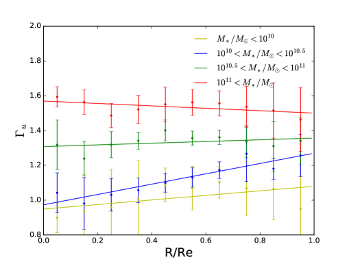
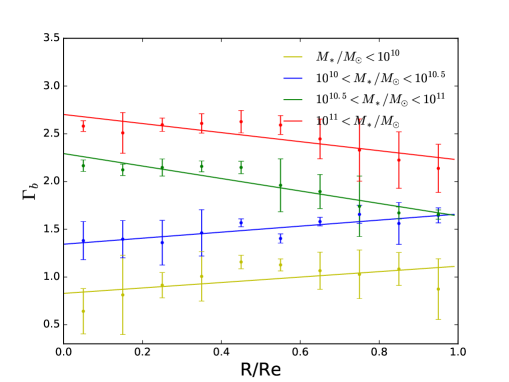
MaNGA IFU data allows us to study possible radial variations of the IMF slope across individual galaxies. Here we carry out such a study by analyzing the radially binned spectra described in §2.4. Results obtained from unimodel and bimodel are shown in Figures 16 and 16, respectively. To estimate the statistical error, we again use the jackknife method to construct 20 jackknife copies. The variance of the IMF slope values estimated from these jackknife copies are shown in the two figures as the error bars.

Figures 16 and 16 show a number of interesting, albeit weak trends. First, at a given $R/R_{e}$ the values of both $\Gamma_{u}$ and $\Gamma_{b}$ increase with stellar mass. This is expected from the results presented in §4.2, as the stellar mass of a galaxy is strongly correlated with its velocity dispersion. Second, for massive ETGs with $M_{*}>10^{10.5}M_{\odot}$, the IMF slope, $\Gamma_{b}$, tends to decrease with increasing radius, suggesting that stars in the inner parts of massive galaxies prefer a bottom heavier IMF than in the outer parts. The trend in $\Gamma_{u}$ is rather weak, but the error bars are larger. Third, for ETGs with $M_{*}<10^{10.5}M_{\odot}$, there seems to be a positive trend of the IMF slope with radius, in that the IMF is steeper in the outer part. For reference, linear fits to the radial gradients are shown as the solid lines in the plots. We have made tests by using stacks according to the velocity dispersion of galaxies, and the results are found to be similar. Negative gradients are found for high velocity dispersion galaxies while the gradients become weaker and even positive for galaxies of low velocity dispersion. The the error bars in the velocity dispersion stacks are smaller than in the stellar mass stacks, especially for high velocity dispersion stacks. This is expected, as stellar population properties in general show tighter correlations with galaxy velocity dispersion than with galaxy mass. However, we only present results for stellar mass stacks, for the convenience of comparison with other results (e.g. Parikh et al., 2018).

The stellar population gradients of ETGs have been discussed in a number of investigations based either on broad-band photometry (e.g. Wu et al., 2005), long-slit spectroscopy (e.g. Sánchez-Blázquez et al., 2007; Spolaor et al., 2009), or IFU data (e.g. Li et al., 2018; Lian et al., 2018). The negative gradient of the IMF slope seen for massive galaxies is consistent with the negative metallicity gradients seen in these analyses. For low-mass ETGs, a relation between stellar mass and metallicity gradient, in that metallicity gradient is shallower for lower masses, is also observed in some earlier studies (e.g. Spolaor et al., 2009; Li et al., 2018; Lian et al., 2018). However, since positive metallicity gradients are observed only in the very low-mass end, the positive IMF gradient observed for low-mass ETGs is difficult to understand. One possibility is that low-mass galaxies have a negative gradient in dust optical depth. The positive gradient in IMF slope can then be generated by the degeneracy of the IMF slope with dust optical depth, in the sense that a lower optical depth leads to to a steeper IMF slope, as shown in Fig. 14. Clearly, a detailed analysis is required to reach an unambiguous conclusion.

4.7 Test of uncertainties

4.7.1 Signal to noise ratio

Figure 17: The variation of IMF slope generated by random noise in different $\sigma_{*}$ bins. Here the IMF slopes are inferred from a set of artificial galaxy spectra in which random noise is added. Blue squares are the mean slopes in the six $\sigma_{*}$ bins, while the error bars show the variations generated by the noise.

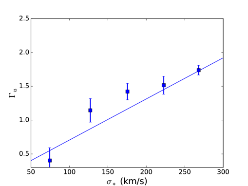
As shown in Figs  8, the scatter in the IMF slope is quite large, particularly for galaxies with low velocity dispersion. It is, therefore, important to test whether such scatter is produced by intrinsic variations or by noise. To do this, we make use of the stacked spectra in different $\sigma_{*}$ bins to examine how the inferred IMF slopes are affected by noise. The stacked spectrum is regarded as noise-free intrinsic spectra for individual galaxies in the corresponding $\sigma_{*}$ bin. Random noises are then added to the spectra according to the noise vectors of individual galaxies to construct an artificial sample. These spectra are then fitted to infer the IMF shapes from the artificial sample. Here the only source of uncertainty in the inferred IMF slope for galaxies in a given $\sigma_{*}$ bin is the difference in the noise vectors and their realizations for individual galaxies in the $\sigma_{*}$ bin. The results for galaxies in different $\sigma_{*}$ bins are shown in Fig. 17. We only plot the inferred IMF slope for unimodel IMF, as bimodel gives very similar results. As one can see, although the global trend in the IMF variation is well recovered from the artificial sample, random noise contributes significantly to the scatter (represented by the bars), especially for low-$\sigma_{*}$ galaxies. This large scatter suggests that the results of the IMF slopes for individual galaxies should be used with caution.

4.7.2 SSP model and abundance ratio

Figure 18: The evidence ratio between Kroupa and Salpeter IMFs plotted against galaxy velocity dispersion, as derived from the C18 model. Each red dot stands for the result of a MaNGA ETG. Blue stars are the median values in five $\sigma_{*}$ bins and connected by a blue line. Error bars are obtained from the jackknife method.

Figure 19: The variation of $\Gamma_{u}$ for galaxies in different $\rm Mgb/\langle Fe\rangle$ bins. The red, green, blue dots stand for galaxies in different $\rm Mgb/\langle Fe\rangle$ bins, as indicated. Big symbols connected by thick lines are results from the stacked spectra in the corresponding $\rm Mgb/\langle Fe\rangle$ bins. Error bars are estimated from the jackknife method.

Figure 20: The relative contribution of the population with Salpeter IMF, $f_{\rm Sal}$, inferred from the E-Miles models with three different [Mg/Fe], as indicated. Error bars are estimated from the jackknife method.

When model uncertainties are ignored, Stellar population parameters recovered from full-spectrum fitting are in general stable if the spectrum has sufficiently high SNR (Ge et al., 2018). However, the SSP model adopted in the fitting can affect the fitting results significantly. The SSP models can differ in a variety of ways, such as stellar templates and isochrones, and even in the method to populate stars in parameter space. In addition, public versions of different SSP models generally have different parameterizations of the IMF for different purposes. All these can potentially affect the inferences of model parameters from the observed spectra. Efforts have been made to ensure the consistency of the IMF inferred from different stellar population models. For example, Spiniello et al. (2015) compare two sets of widely-used SSP models to demonstrate the non-universality of the IMF in the low-mass end, and conclude that the non-universality of the IMF is robust against the choice of SSP model. For the MaNGA data, Parikh et al. (2018) use two different SSP models, VCJ (Villaume et al., 2017a) and M11-MARCS (Maraston & Strömbäck, 2011; Gustafsson et al., 2008), to fit IMF-sensitive line indexes in the near infrared spectral region, and obtain qualitatively consistent results. All these indicate that different SSP models agree with each other in general, while discrepancy may exists between models in detail.

Since these results are all based on absorption lines, it remains unclear whether or not our results based on full spectrum fitting can be affected significantly by our adopted SSP model. To test this, we carry out an analysis by using the SSP model presented in Conroy et al. (2018) (referred to as C18 model) instead of the E-MILES model. Different from E-MILES model, C18 is constructed from the MILES and Extended IRTF libraries and has a number of free parameters to describe the variations in element abundance patterns but only provides a limited choices for the IMF. To make a fair comparison with Fig. 6, we restrict our analysis to the base C18 model, which assumes solar abundance pattern and Salpeter and Kroupa IMFs, neglecting all the free parameters that account for element abundance variations. These SSP models are then used to fit the stacked spectra, as was done in Fig. 6, and the resulting evidence ratio between the Kroupa and Salpeter IMF models, $\ln(E_{K}/E_{S})$, versus $\sigma_{*}$ is shown in Fig.  18. Comparing the result with that shown in Fig. 6, we see that the trend that the Salpeter IMF is preferred by high-mass ETGs are not affected significantly by the change of the SSP model.

Another potential uncertainty comes from possible variations of the element abundance pattern from galaxy to galaxy. It is easy to understand that the inference of the IMF from absorption line analysis is sensitive to the abundances of individual elements, especially those whose absorption lines are used (e.g. [Na/Fe]). In the full spectrum fitting adopted here, the problem may be alleviated, as the influence of the variation of individual element abundances is generally limited to specific wavelength ranges. However, a systematic variation of a group of elements, such as the $\alpha$ elements, may still cause significant difference in the continuum, thereby affecting our inferences for the IMF shape. Moreover, elliptical galaxies are known to be $\alpha$-enhanced (e.g. Trager et al., 2000), while the E-MILES templates adopted here are constructed with the solar abundance pattern. It is therefore necessary to test whether our inferences are affected significantly by the change of the abundance ratio.

The lick index ratio ${\rm Mgb/\langle Fe\rangle}\equiv\rm 2Mgb/(Fe5270+Fe5335)$ has been widely used as a good indicator for the $\alpha$-abundance, especially for old populations (ages above $\sim 8$ Gyr,Thomas et al. 2003). Fig. 19 shows results for galaxies divided into three bins according to their ${\rm Mgb/\langle Fe\rangle}$. It is clear from the plot that the trends of the IMF slope with velocity dispersion are similar without strong dependence on ${\rm Mgb/\langle Fe\rangle}$, indicating that our results are insensitive to the assumed element abundance pattern. We have also examined the same correlations as shown in Fig. 19 but using $\alpha$-abundance estimates of Zheng et al. (2019) obtained from SPS models. Although not shown here, the trends obtained are very similar to those shown in Fig. 19.

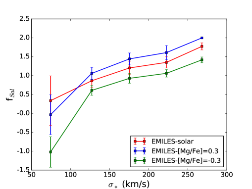
A more direct way to check the impact of abundance ratio is to use SSP models with varying abundance ratios. Unfortunately, E-MILES does not provide templates with different [$\alpha$/Fe] or other abundance ratios. As an alternative test, we use the response functions from Conroy et al. (2018) to construct models with different abundance patterns. The response functions are ratios between the SSPs generated with stellar templates with varied abundance for a single element and those generated with the standard abundance patterns. SSP models with different abundance patterns can then be generated by multiplying those response functions with the original model. These functions cover a wide range in metallicity ($-1.5<{\rm[Fe/H]}<0.3$), and are appropriate for old stellar populations with ages $>1{\rm Gyr}$. Among all the element abundance variations, that of [Mg/Fe] is the easiest to measure and has significant impact on the spectral shape. As a preliminary test, we use the response function of Mg/Fe from Conroy et al. (2018), which is given for [Mg/Fe]=$\pm 0.3$, to generate two perturbed E-MILES models. As the response function is available only for a limited number of IMF models, we focus on the widely used Kroupa and Salpeter IMFs. To quantify the IMF variation, we model a given spectrum with $F=(f_{\rm Sal})\times F_{{\rm Sal}}+(1-f_{\rm Sal})\times F_{\rm Krp}$, where $F_{\rm Sal}$ and $F_{\rm Krp}$ are spectral fluxes predicted with a given set of parameters but from SSPs assuming Salpeter and Kroupa IMFs, respectively. The parameter $f_{\rm Sal}$, which can be interpreted as the relative contribution of the population with a Salpeter IMF, then takes the place of the IMF slope used in previous sections to characterize the IMF shape. As $f_{\rm Sal}$ is used to form a linear combination of the two IMFs, the value of $f_{\rm Sal}$ is allowed to be bigger than one and smaller than zero.

The three SSP models, namely the original E-MILES model, and the two perturbed models with ${\rm[Mg/Fe]}=\pm 0.3$, are then used to fit the the stacked spectra, and the results are shown in Fig. 20. It can be seen that $f_{\rm Sal}$ is positively correlated with $\sigma_{*}$ for all the three assumptions of ${\rm[Mg/Fe]}$, indicating again a bottom-heavier IMF for more massive ETGs. Comparing results of different ${\rm[Mg/Fe]}$, we see that the value of $f_{\rm Sal}$ increases systematically with the abundance ratio ${\rm[Mg/Fe]}$. However, the overall trend of $f_{\rm Sal}$ with $\sigma_{*}$ remains unchanged by the change in ${\rm[Mg/Fe]}$. Since ${\rm[Mg/Fe]}$ is not expected to be anti-correlated with $\sigma_{*}$ (see Zheng et al., 2019) for the MaNGA galaxies, the trends seen in Fig. 8 are robust against [Mg/Fe] variations.

This test can be applied to all the available element abundance variations separately. Although not shown in the paper, we have done the same tests for abundance ratios like [Na/Fe] and [Ca/Fe], and found that the impact of these variations are much smaller. One can in principle include all abundance ratios simultaneously under the assumption that the responses from different elements are uncorrelated. In fact, such an approach has already been adopted in some earlier IMF investigations (e.g. Conroy & van Dokkum, 2012b; Villaume et al., 2017b). However, as our Bayesian analysis needs to estimate multi-dimensional integrations to obtain the global evidence for a large sample of ETGs, it is extremely time consuming to include all possible abundance variations in the fitting. Furthermore, although we have limited to Salpeter and Kruopa IMFs to avoid differences in the IMF parameterization, the E-MILES and C18 models may have other differences that have not been explored, and it is unclear whether the response functions taken from C18 are accurate for E-MILES. As our tests show that our conclusions are not affected significantly by element abundance variations, we will not explore this issue in more detail.

4.7.3 Star formation history

Our inferences presented above assume that the star formation histories (SFH) of individual galaxies can be described by the $\Gamma$ function model, equation (3). This may be a good approximation for massive elliptical galaxies, where stellar populations are old and more or less uniform. For low-mass galaxies, however, the star formation histories may be more complex. To test the effects of the assumed star formation histories on our inferences of IMF slopes, we have run a set of spectral fitting by assuming the widely used $\tau$ model, referred to as $\tau$-SFH, which can be written as

$$\Psi(t)=\frac{1}{\tau}\frac{e^{-t/\tau}}{1-e^{-\Delta t/\tau}}$$ (9)

where $\tau$ is the star formation time scale and $\Delta t$ is the time span over which star formation occurs. We find that the results obtained by using the $\tau$-SFH are all consistent with the results obtained from the $\Gamma$-SFH, indicating that our results are not affected significantly by the change of the SFH model.

In addition to the two continuous star formation histories, we have also tested whether or not an additional burst population is needed by the data. By comparing the evidence ratio between models of the $\Gamma$-SFH with and without the additional burst, we find that the majority of the galaxies do not show a preference for an additional stellar population. In summary, the SFH model adopted in our analysis is sufficient for our purpose. A more detailed modeling of the SFH may improve the inferences for some galaxies, but it will not affect our main conclusions.

5 Comparison with earlier results

Our analysis is based on the MaNGA data and fitting to the full spectra. It is complementary to earlier studies based on different methods and datasets. In this section, we compare our results with those obtained before.

5.1 The IMF slope

Our analysis reveals a positive correlation between the IMF slope, which describes the relative ratio between low-mass and high mass stars, and the central stellar velocity dispersion for ETGs over a large range of velocity dispersion, $\sigma_{*}\approx 50-350$  km s^-1. This excess of low mass stars in high mass ETGs is also supported by Bayesian model selections between a Milky Way like IMF and a bottom-heavy IMF. This correlation has been found earlier in a number of investigations (e.g. Thomas et al., 2011; Dutton et al., 2012; Cappellari et al., 2012; Conroy & van Dokkum, 2012b; Spiniello et al., 2012; Ferreras et al., 2013; La Barbera et al., 2013; Posacki et al., 2015; Lyubenova et al., 2016; Li et al., 2017; Villaume et al., 2017b; Parikh et al., 2018). Among these, Ferreras et al. (2013) used a SSP model family (the MIUSCAT SSP models, a progenitor of E-MILES) similar to what is adopted here, to analyze the stacked spectra from SDSS for galaxies with $\sigma_{*}>150$  km s^-1. Their results, obtained from TiO1, TiO2 and Na8190 absorption features versus ours based on full spectrum fitting, are in quantitative agreement, suggesting consistencies in the two approaches. However, the single fiber spectroscopy did not allow them to investigate possible IMF variations within individual galaxies.

La Barbera et al. (2013) also used the MIUSCAT SSP models to study the IMF variation, taking into account possible non-solar abundance. Their spectral analyses did not seem to be able to discriminate a single power law (unimodal) IMF from a low-mass ($<0.5M_{\odot}$) tapered (bimodal) IMF, in contrast to our Bayesian analysis that clearly favours unimodal IMF, especially for high mass ETGs. However, if dynamical constraints are taken into account, as discussed in La Barbera et al. (2013), unimodal IMF models can lead to unrealistic mass-to-light ratios that are too large to be consistent with dynamical measurements, while bimodal IMF models well meet the dynamical constrains. Similar results were reported in Lyubenova et al. (2016) by comparing dynamical modeling and stellar population results obtained from applying E-MILES models to CALIFA data. The tension between stellar population and dynamical results is likely due to issues in IMF parameterizations. In fact, as shown in Conroy & van Dokkum (2012b), a three component power-law IMF with slope varying at the low mass end ($0.1M_{\odot}<M<0.5M_{\odot}$ and $0.5M_{\odot}<M<1.M_{\odot}$) but fixed at the high mass end ($>1M_{\odot}$), seems to be able to fit the absorption features in ETGs and to satisfy dynamical constraints simultaneously. Unfortunately, the bimodal IMF adopted here does not really have the flexibility at the low-mass end. We suspect that this is the reason why the uimodal IMF is preferred in our analysis. Because of the single IMF slope over the entire mass range, the uimodal IMF may fail to reproduce the mass-to-light ratios of galaxies. Unfortunately, the lack of a more flexible IMF parameterization in E-MILES model prevent us from investigating this issue further.

Parikh et al. (2018) used a MaNGA data set similar to the one used here to investigate variations of the IMF. Their analysis was based on the absorption lines, NaI and FeH, and the SSP templates of VCJ (Villaume et al., 2017a) and M11-MARCS (Maraston & Strömbäck, 2011; Gustafsson et al., 2008), different from the E-MILES templates adopted here. The general trend they found, that the type of IMF seems to change from low mass to high mass ETGs, is similar to what is found here, indicating that the results are not sensitive to the SSP models adopted. However, the radial gradients in the IMF slope they found are quite different from what we obtain here, as to be described in more detail below (§5.2).

In addition to the correlation between the IMF slope and $\sigma_{*}$, other types of correlation, especially the IMF-metallicity correlation, have also been suggested. For example, studies of Wolf-Rayet stars indicate a correlation between gas phase metallicity and IMF (Zhang et al., 2007), and direct star counts in nearby resolved galaxies (Geha et al., 2013) give a similar correlation between IMF and stellar metallicity. Such a correlation is also revealed in the study of 24 CALIFA galaxies by Martín-Navarro et al. (2015b), who found that the correlation of the IMF shape, $\Gamma_{b}$, with galaxy metallicity is the strongest among the correlations with a number of other galaxy properties, such as velocity dispersion. Similar conclusion was reached by Parikh et al. (2018) using radially stacked spectra of MaNGA galaxies. Villaume et al. (2017b) studied a parameter, $\alpha_{\rm IMF}$, which is the ratio of the stellar mass-to-light ratio, $(M/L)_{*}$, obtained from fitting with varying IMF, to the value of $(M/L)_{*}$ obtained with a MW IMF, and its correlation with [Fe/H], [Mg/Fe] and $\sigma_{*}$, for a sample that includes ETG galaxies from van Dokkum et al. (2017), three M31 globular clusters, one ultra-compact dwarf, and M32. They found that the IMF variation is most tightly correlated with [Fe/H]. Our results confirm these results with a much larger sample covering a larger dynamic range. In particular, our Bayesian approach allows us to examine in detail the covariance and degeneracy in the various correlations seen in the data. Villaume et al. (2017a) also found a globular cluster that deviates significantly from the global trend, and suggested that metallicity is not the sole driver of IMF variation.

From a theoretical point of view, the thermal properties of star-forming clouds are expected to have important influences on how they fragment into stars, which can, in turn, affect the stellar IMF (Larson, 2005). Since the abundances of atoms, molecules, and dust grains are responsible for the cooling, the overall metallicity is expected to play an important role in shaping the IMF. However, only limited attempts have been made in quantifying the effect of metallicity on the thermal properties of collapsing clouds (e.g. Low & Lynden-Bell, 1976; Omukai, 2000). As our results provide strong evidence that metallicity is the dominant driver of IMF variations, which is consistent with other studies mentioned above, we expect to see further studies of the thermal properties of star-forming clouds in different circumstances and how the stellar IMF can be affected by metallicity.

Finally, a completely different approach, based on dynamical modeling of MaNGA galaxies, has been adopted by Li et al. (2017) to constrain potential IMF variations. The dynamical modeling provided constraints on the stellar mass to light ratio of galaxies as a function of galaxy velocity dispersion, which were then compared to the expected mass to light ratios from different IMFs. The trend they found is qualitatively the same as found here, in that galaxies with higher velocity dispersion tend to prefer a bottom-heavier IMF. However, as the kinematic results can only provide an overall constraint on the stellar mass to light ratio, they may be subjected to a different set of uncertainties, such as the uncertainty in the modeling of dark matter distribution, and the degeneracy between IMF and star formation history in the mass-to-light ratio. Because of this, a quantitative comparison between their results and ours is difficult to make.

5.2 Radial dependence

Thanks to the spatially resolved IFU spectra provided by MaNGA, we are able to derive radial gradients from a set of stacked spectra. Our results show a difference in the radial gradient, from a negative gradient to a positive gradient in the IMF slope, between massive ETGs with $M_{*}$ larger or smaller than $10^{10.5}M_{\odot}$. A number of earlier investigations have reported the presence of IMF gradients indicating dwarf-richer stellar populations towards the centers of massive ETGs (e.g. Martín-Navarro et al., 2015a; La Barbera et al., 2017; van Dokkum et al., 2017; Vaughan et al., 2018b; Sarzi et al., 2018; Parikh et al., 2018), with the exceptions in some other investigations (Vaughan et al., 2018a; Zieleniewski et al., 2015, 2017; McConnell et al., 2016; Alton et al., 2017).

Many of the earlier investigations of the IMF gradient are based on small samples, as IFU observations are relatively rare. Martín-Navarro et al. (2015a), for example, studied the radial gradients of the IMF slope, $\Gamma_{b}$, for three early-type galaxies with central velocity dispersion $\sigma_{*}\approx 300$, $280$, and $100$  km s^-1, respectively, and found strong enhancements of low mass stars in the central parts of the two large galaxies, but a flat or slightly opposite trend for the galaxy with the lowest $\sigma_{*}$. Their results are based on spectral indices including TiO1, TiO2, NaD and NaI8190. Although the last two indexes may be affected by sky emission and telluric absorption, the trends they found for the three galaxies are in good agreement with our results. A similar analyses, carried out by La Barbera et al. (2017) using spectra indices in redder bands, showed that IMF varies with radius in two nearby massive ETGs with $\sigma_{*}\approx 300$  km s^-1. van Dokkum et al. (2017) studied six ETGs with $\sigma_{*}$ ranging from 163 to 340  km s^-1, using IMF-sensitive absorption lines instead of spectral indexes. After accounting for element abundance gradients, they were able to find strong enhancements of low mass stars in the central parts of all the six galaxies.

Compared to these case studies using small number of galaxies, large IFU surveys are complementary and particularly suitable for statistical analyses. However, observational samples have been quite limited up to now. Martín-Navarro et al. (2015b) analyzed a sample of 24 ETGs with $\sigma_{*}$ ranging from 160 to 310  km s^-1and a mean stellar mass $10^{11.54}M_{\odot}$, drawn from the CALIFA (Sánchez et al., 2012) IFU survey. They found that the local IMF within a galaxy is tightly correlated with the local metallicity, being bottom-heavier for metal-richer populations. As ETGs generally have negative gradients in metallicity, their results imply a IMF gradient in massive galaxies in the same way as we find.

As mentioned above, Parikh et al. (2018) used a set of MaNGA galaxies similar to ours to study radial gradients of IMF by modeling absorption line indices. Their analysis based on NaI index and the M11-MARCS stellar population model revealed a significant negative gradient in massive galaxies, while a much weaker gradient is found for low-mass galaxies. This is in good agreement with ours, suggesting a difference in IMF gradient between high and low mass galaxies. However, their analysis of the same index but using the VCJ stellar population model shows a significant negative gradient also for low-mass galaxies. This suggests that the evolution of low-mass galaxies may be more complex, and thus is more challenging to model. More surprisingly, their analysis of another IMF-sensitive index, FeH at around 9900Å, using either of the two SSP models, revealed strong positive radial gradients in the IMF slope, in conflict with their results based on the NaI index and the results we obtain. This may arise from the difficulty in modelling reliably the FeH index. Our fitting does not cover that spectral region, and thus would not suffer from this inconsistency.

While many previous studies have found evidences for the presence of negative IMF gradients, a few of the investigations questioned the significance of such gradients. These investigations generally did find radial gradients in absorption features. However, the gradients can be interpreted as those in element abundance. For example, Alton et al. (2017) studied eight early-type galaxies with $\sigma_{*}\approx 250$ observed in $0.8-1.35{\rm\mu m}$, and concluded that the measured radial changes in absorption feature strengths can be explained entirely by abundance gradients. In addition, they found that the fractional contribution of dwarf stars to the $J$-band total flux, which is believed to be closely related to the IMF, also provides no clear evidence for radial variations of the IMF. However, the validity of their inference of low-mass star fraction can be limited by the wavelength coverage, as it can be affected by uncertainties in age and metallicity. Additional information, such as spectral indexes or spectra covering shorter wavelengths, may be needed to break the degeneracy (e.g. Vaughan et al., 2018a).

In conclusion, the radial dependence of the IMF we find for ETGs is consistent with some of the earlier results. The fact that there is significant variation in the IMF shape among individual galaxies of similar $\sigma_{*}$ and that the radial IMF gradient on average depends on galaxy mass suggests that some of the discrepancies seen in earlier results may be due to such variation and dependence.

6 Summary and discussion

We use a Bayesian inference code to analyze the spectra of a sample of ETGs selected from the SDSS-IV MaNGA IFU survey and to study possible variations in their IMF. High SNR spectra of individual galaxies are obtained by stacking the spatially resolved spectra within $1.0R_{e}$, as well as by radially stacked spectra for a sample of galaxies in given stellar mass bins. Our analysis is based on full spectrum fitting, making use of the MaNGA spectra from 3400 Å to 8900 Å, while masking the problematic region (6800 Å to 8100 Å). The state-of-the-art E-MILES synthetic stellar population models, with two types of IMF parameterizations, unimodel and bimodel, are used to infer the IMF slope from the spectra, while the widely used Chabrier and Salpeter IMFs are tested with Bayesian model selections. Our main results can be summarized as follows:

• The IMF is not universal among ETGs, as indicated by the evidence ratio between different types of IMF. A clear trend of the evidence ratio between Chabrier and Salpeter IMFs with galaxy velocity dispersion, $\sigma_{*}$, shows that the Salpeter IMF becomes more favored over the Chabrier IMF for higher mass ETGs. In addition, the unimodel model family, which is described by a single power law, is also favored by massive ETGs over a model family in which the IMF is assumed to flatten in the low-mass end. All these suggest that Galactic-like IMF may be invalid for high-mass ETGs.

• The IMF slope inferred from our full spectra fitting follows a clear trend with central velocity dispersion $\sigma_{*}$, in the sense that galaxies of higher $\sigma_{*}$ on average have IMFs that are more bottom-heavy. However, this correlation is driven by the dependence of IMF shape on metallicity, as galaxies of similar metallicities have only weak dependence on $\sigma_{*}$.

• The degeneracy between metallicity, age and dust extinction of a galaxy can induce systematic trends in the IMF slope with stellar age and dust optical depth. The dependence of the IMF slope on these parameters is through a combination, $D$ that is perpendicular to the degeneracy direction.

• Using age and metallicity estimates in which the degeneracy between them is reduced, and their scaling relations with galaxy velocity dispersion, we found the the IMF variations can be explained entirely by metallicity variations, but not by age variations.

• We found a weak negative gradient in the IMF slope in individual galaxies, in the sense that the IMF in the center of a massive ETG is, on average, more bottom-heavy than in the outer part, while a weak opposite tend is found for low-mass ETGs. This dependence of IMF radial gradient on galaxy mass suggests that part of the discrepancies seen in earlier results may be due to such dependence

• We tested all the trends found in the paper with both IMF parameterizations, unimodel and bimodel, and found no significant differences. In addition, we also tested the robustness of our results against a number of uncertainties, such as the variation in spectral signal-to-noise ratio, stellar population models with varying abundance ratios, and the modelling of star formation histories.

Our investigation is one of the first attempts to use full spectrum fitting to constrain the IMF shape of galaxies. With the help of Bayesian analysis, we are able to compare different IMF model families, as well as to examine how the inferred IMF slopes are affected by the degeneracy with other model parameters. This is a novel approach to the problem, and here we discuss further some of the potentials and pitfalls of the method.

Compared to absorbtion line analysis, the full spectrum fitting method makes use of more information contained in the spectra. This allows one to determine the IMF shape together with other properties, such as stellar age, metallicities, dust attenuations, and to examine their covariance. In fact, some earlier studies (e.g. Ferreras et al., 2013) have used the optical spectra to measure auxiliary galaxies properties in addition to the IMF. The Bayesian approach adopted here is a statistically more rigorous way to make self-consistent inferences from the full spectra. As shown in the paper, the IMF slope and its covariance with stellar age, metallicity and dust extinction can be quantified in the Bayesian approach. In particular, the covariance is found to be only modest, and does not hinder the inferences of the IMF shape.

An issue in absorption line analysis is that it can be affected significantly by the abundance variations of certain elements. Detailed theoretical modelling of a small number of absorbtion features is possible (e.g. Conroy & van Dokkum, 2012a; Conroy et al., 2018), and may help to take into account such abundance variations. In full spectrum fitting, however, theoretical templates are not commonly used, as it is hard to model the large number of spectral features in the whole spectra. Currently, the lack of observed stellar templates of varying element abundance patterns weakens the abilities of full spectrum fitting in inferring the abundance of elements that might be related to the IMF. However, the influence of element abundance variations is generally confined to certain spectral regions, and their effects on IMF inferences based on full spectrum fitting are reduced, as demonstrated by our tests. Nevertheless, it should be emphasized that a detailed analysis of abundance ratios is needed in order to make accurate inferences of the IMF shape, and to quantify the covariance between IMF shape and abundance ratio.

Since IMF variation has the greatest impact in the near infrared parts of galaxy spectra and the effect is in general small, modeling the effect is a challenge to the spectral population synthesis model. Most of the stellar templates currently available (e.g. MILES) have proper coverage only in optical, and need to be matched with other stellar libraries to construct SSPs with appropriate spectral coverage. Such a match can be made only when fluxes in different wavelength ranges are calibrated properly. Some investigators have chosen to split the spectra into pieces and fit the local continuum (e.g. van Dokkum et al., 2017; Vaughan et al., 2018a), while we have used a carefully designed mask to get rid of problematic spectral portions. Both methods may have their own uncertainties. The fact that these approaches produce consistent results indicates that the inferences of IMF variations are robust against such uncertainties. In the future, when stellar templates with higher resolution and wider spectral coverage, such as the MaSTAR (Yan & MaStar Team, 2017), become available, our method should be able to provide an even more powerful tool to investigate IMF variations.

References

- Abolfathi et al. (2018) Abolfathi B., et al., 2018, ApJS, 235, 42
- Alton et al. (2017) Alton P. D., Smith R. J., Lucey J. R., 2017, MNRAS, 468, 1594
- Barber et al. (2018) Barber C., Crain R. A., Schaye J., 2018, MNRAS, 479, 5448
- Barber et al. (2019a) Barber C., Schaye J., Crain R. A., 2019a, MNRAS, 482, 2515
- Barber et al. (2019b) Barber C., Schaye J., Crain R. A., 2019b, MNRAS, 483, 985
- Blanton & Roweis (2007) Blanton M. R., Roweis S., 2007, AJ, 133, 734
- Blanton et al. (2005) Blanton M. R., et al., 2005, AJ, 129, 2562
- Blanton et al. (2017) Blanton M. R., et al., 2017, AJ, 154, 28
- Bruzual & Charlot (2003) Bruzual G., Charlot S., 2003, MNRAS, 344, 1000
- Bundy et al. (2015) Bundy K., et al., 2015, ApJ, 798, 7
- Calzetti et al. (2000) Calzetti D., Armus L., Bohlin R. C., Kinney A. L., Koornneef J., Storchi-Bergmann T., 2000, ApJ, 533, 682
- Cappellari (2017) Cappellari M., 2017, MNRAS, 466, 798
- Cappellari & Emsellem (2004) Cappellari M., Emsellem E., 2004, PASP, 116, 138
- Cappellari et al. (2012) Cappellari M., et al., 2012, Nature, 484, 485
- Cappellari et al. (2013) Cappellari M., et al., 2013, MNRAS, 432, 1862
- Cenarro et al. (2001) Cenarro A. J., Cardiel N., Gorgas J., Peletier R. F., Vazdekis A., Prada F., 2001, MNRAS, 326, 959
- Cenarro et al. (2003) Cenarro A. J., Gorgas J., Vazdekis A., Cardiel N., Peletier R. F., 2003, MNRAS, 339, L12
- Chabrier (2003) Chabrier G., 2003, PASP, 115, 763
- Chabrier et al. (2014) Chabrier G., Hennebelle P., Charlot S., 2014, ApJ, 796, 75
- Charlot & Fall (2000) Charlot S., Fall S. M., 2000, ApJ, 539, 718
- Cid Fernandes et al. (2005) Cid Fernandes R., Mateus A., Sodré L., Stasińska G., Gomes J. M., 2005, MNRAS, 358, 363
- Clauwens et al. (2016) Clauwens B., Schaye J., Franx M., 2016, MNRAS, 462, 2832
- Collier et al. (2018) Collier W. P., Smith R. J., Lucey J. R., 2018, MNRAS, 478, 1595
- Conroy (2013) Conroy C., 2013, ARA&A, 51, 393
- Conroy & van Dokkum (2012a) Conroy C., van Dokkum P., 2012a, ApJ, 747, 69
- Conroy & van Dokkum (2012b) Conroy C., van Dokkum P. G., 2012b, ApJ, 760, 71
- Conroy et al. (2018) Conroy C., Villaume A., van Dokkum P. G., Lind K., 2018, ApJ, 854, 139
- Cushing et al. (2005) Cushing M. C., Rayner J. T., Vacca W. D., 2005, ApJ, 623, 1115
- De Masi et al. (2018) De Masi C., Matteucci F., Vincenzo F., 2018, MNRAS, 474, 5259
- Drory et al. (2015) Drory N., et al., 2015, AJ, 149, 77
- Dutton et al. (2012) Dutton A. A., Mendel J. T., Simard L., 2012, MNRAS, 422, L33
- Emsellem et al. (2004) Emsellem E., et al., 2004, MNRAS, 352, 721
- Feroz et al. (2009) Feroz F., Hobson M. P., Bridges M., 2009, MNRAS, 398, 1601
- Feroz et al. (2013) Feroz F., Hobson M. P., Cameron E., Pettitt A. N., 2013, preprint, (arXiv:1306.2144)
- Ferreras et al. (2013) Ferreras I., La Barbera F., de la Rosa I. G., Vazdekis A., de Carvalho R. R., Falcón-Barroso J., Ricciardelli E., 2013, MNRAS, 429, L15
- Ferreras et al. (2015) Ferreras I., Weidner C., Vazdekis A., La Barbera F., 2015, MNRAS, 448, L82
- Fischer et al. (2019) Fischer J.-L., Domínguez Sánchez H., Bernardi M., 2019, MNRAS, 483, 2057
- Gallazzi et al. (2005) Gallazzi A., Charlot S., Brinchmann J., White S. D. M., Tremonti C. A., 2005, MNRAS, 362, 41
- Ge et al. (2018) Ge J., Yan R., Cappellari M., Mao S., Li H., Lu Y., 2018, MNRAS, 478, 2633
- Geha et al. (2013) Geha M., et al., 2013, ApJ, 771, 29
- Gunawardhana et al. (2011) Gunawardhana M. L. P., et al., 2011, MNRAS, 415, 1647
- Gunn et al. (2006) Gunn J. E., et al., 2006, AJ, 131, 2332
- Gustafsson et al. (2008) Gustafsson B., Edvardsson B., Eriksson K., Jørgensen U. G., Nordlund Å., Plez B., 2008, A&A, 486, 951
- Gutcke & Springel (2019) Gutcke T. A., Springel V., 2019, MNRAS, 482, 118
- Jeřábková et al. (2018) Jeřábková T., Hasani Zonoozi A., Kroupa P., Beccari G., Yan Z., Vazdekis A., Zhang Z.-Y., 2018, A&A, 620, A39
- Kroupa (2001) Kroupa P., 2001, MNRAS, 322, 231
- La Barbera et al. (2013) La Barbera F., Ferreras I., Vazdekis A., de la Rosa I. G., de Carvalho R. R., Trevisan M., Falcón-Barroso J., Ricciardelli E., 2013, MNRAS, 433, 3017
- La Barbera et al. (2015) La Barbera F., Ferreras I., Vazdekis A., 2015, MNRAS, 449, L137
- La Barbera et al. (2017) La Barbera F., Vazdekis A., Ferreras I., Pasquali A., Allende Prieto C., Röck B., Aguado D. S., Peletier R. F., 2017, MNRAS, 464, 3597
- Larson (2005) Larson R. B., 2005, MNRAS, 359, 211
- Law et al. (2015) Law D. R., et al., 2015, AJ, 150, 19
- Law et al. (2016) Law D. R., et al., 2016, AJ, 152, 83
- Li et al. (2017) Li H., et al., 2017, ApJ, 838, 77
- Li et al. (2018) Li H., et al., 2018, MNRAS, 476, 1765
- Lian et al. (2018) Lian J., et al., 2018, MNRAS, 476, 3883
- Low & Lynden-Bell (1976) Low C., Lynden-Bell D., 1976, MNRAS, 176, 367
- Lu et al. (2015) Lu Z., Mo H. J., Lu Y., Katz N., Weinberg M. D., van den Bosch F. C., Yang X., 2015, MNRAS, 450, 1604
- Lyubenova et al. (2016) Lyubenova M., et al., 2016, MNRAS, 463, 3220
- Maraston (1998) Maraston C., 1998, MNRAS, 300, 872
- Maraston (2005) Maraston C., 2005, MNRAS, 362, 799
- Maraston & Strömbäck (2011) Maraston C., Strömbäck G., 2011, MNRAS, 418, 2785
- Martín-Navarro et al. (2015a) Martín-Navarro I., La Barbera F., Vazdekis A., Falcón-Barroso J., Ferreras I., 2015a, MNRAS, 447, 1033
- Martín-Navarro et al. (2015b) Martín-Navarro I., et al., 2015b, ApJ, 806, L31
- McConnell et al. (2016) McConnell N. J., Lu J. R., Mann A. W., 2016, ApJ, 821, 39
- Meurer et al. (2009) Meurer G. R., et al., 2009, ApJ, 695, 765
- Newman et al. (2017) Newman A. B., Smith R. J., Conroy C., Villaume A., van Dokkum P., 2017, ApJ, 845, 157
- Omukai (2000) Omukai K., 2000, ApJ, 534, 809
- Parikh et al. (2018) Parikh T., et al., 2018, MNRAS, 477, 3954
- Posacki et al. (2015) Posacki S., Cappellari M., Treu T., Pellegrini S., Ciotti L., 2015, MNRAS, 446, 493
- Rayner et al. (2009) Rayner J. T., Cushing M. C., Vacca W. D., 2009, ApJS, 185, 289
- Salpeter (1955) Salpeter E. E., 1955, ApJ, 121, 161
- Sánchez-Blázquez et al. (2006) Sánchez-Blázquez P., et al., 2006, MNRAS, 371, 703
- Sánchez-Blázquez et al. (2007) Sánchez-Blázquez P., Forbes D. A., Strader J., Brodie J., Proctor R., 2007, MNRAS, 377, 759
- Sánchez et al. (2012) Sánchez S. F., et al., 2012, A&A, 538, A8
- Sarzi et al. (2018) Sarzi M., Spiniello C., La Barbera F., Krajnović D., van den Bosch R., 2018, MNRAS, 478, 4084
- Smee et al. (2013) Smee S. A., et al., 2013, AJ, 146, 32
- Smith & Lucey (2013) Smith R. J., Lucey J. R., 2013, MNRAS, 434, 1964
- Smith et al. (2015) Smith R. J., Lucey J. R., Conroy C., 2015, MNRAS, 449, 3441
- Spiniello et al. (2012) Spiniello C., Trager S. C., Koopmans L. V. E., Chen Y. P., 2012, ApJ, 753, L32
- Spiniello et al. (2014) Spiniello C., Trager S., Koopmans L. V. E., Conroy C., 2014, MNRAS, 438, 1483
- Spiniello et al. (2015) Spiniello C., Trager S. C., Koopmans L. V. E., 2015, ApJ, 803, 87
- Spolaor et al. (2009) Spolaor M., Proctor R. N., Forbes D. A., Couch W. J., 2009, ApJ, 691, L138
- Thomas et al. (2003) Thomas D., Maraston C., Bender R., 2003, MNRAS, 339, 897
- Thomas et al. (2005) Thomas D., Maraston C., Bender R., Mendes de Oliveira C., 2005, ApJ, 621, 673
- Thomas et al. (2011) Thomas J., et al., 2011, MNRAS, 415, 545
- Trager et al. (2000) Trager S. C., Faber S. M., Worthey G., González J. J., 2000, AJ, 119, 1645
- Treu et al. (2010) Treu T., Auger M. W., Koopmans L. V. E., Gavazzi R., Marshall P. J., Bolton A. S., 2010, ApJ, 709, 1195
- Valdes et al. (2004) Valdes F., Gupta R., Rose J. A., Singh H. P., Bell D. J., 2004, ApJS, 152, 251
- Vaughan et al. (2018a) Vaughan S. P., Davies R. L., Zieleniewski S., Houghton R. C. W., 2018a, MNRAS, 475, 1073
- Vaughan et al. (2018b) Vaughan S. P., Davies R. L., Zieleniewski S., Houghton R. C. W., 2018b, MNRAS, 479, 2443
- Vazdekis et al. (1996) Vazdekis A., Casuso E., Peletier R. F., Beckman J. E., 1996, ApJS, 106, 307
- Vazdekis et al. (2010) Vazdekis A., Sánchez-Blázquez P., Falcón-Barroso J., Cenarro A. J., Beasley M. A., Cardiel N., Gorgas J., Peletier R. F., 2010, MNRAS, 404, 1639
- Vazdekis et al. (2016) Vazdekis A., Koleva M., Ricciardelli E., Röck B., Falcón-Barroso J., 2016, MNRAS, 463, 3409
- Villaume et al. (2017a) Villaume A., Conroy C., Johnson B., Rayner J., Mann A. W., van Dokkum P., 2017a, ApJS, 230, 23
- Villaume et al. (2017b) Villaume A., Brodie J., Conroy C., Romanowsky A. J., van Dokkum P., 2017b, ApJ, 850, L14
- Wake et al. (2017) Wake D. A., et al., 2017, AJ, 154, 86
- Wang et al. (2018) Wang E., et al., 2018, ApJ, 856, 137
- Weidner et al. (2013) Weidner C., Ferreras I., Vazdekis A., La Barbera F., 2013, MNRAS, 435, 2274
- Willett et al. (2013) Willett K. W., et al., 2013, MNRAS, 435, 2835
- Worthey (1994) Worthey G., 1994, ApJS, 95, 107
- Wu et al. (2005) Wu H., Shao Z., Mo H. J., Xia X., Deng Z., 2005, ApJ, 622, 244
- Yan & MaStar Team (2017) Yan R., MaStar Team 2017, in Astronomical Society of India Conference Series. pp 99–103 (arXiv:1708.04688)
- Yan et al. (2016a) Yan R., et al., 2016a, AJ, 151, 8
- Yan et al. (2016b) Yan R., et al., 2016b, AJ, 152, 197
- Zhang et al. (2007) Zhang W., Kong X., Li C., Zhou H.-Y., Cheng F.-Z., 2007, ApJ, 655, 851
- Zheng et al. (2019) Zheng Z., et al., 2019, ApJ, 873, 63
- Zieleniewski et al. (2015) Zieleniewski S., Houghton R. C. W., Thatte N., Davies R. L., 2015, MNRAS, 452, 597
- Zieleniewski et al. (2017) Zieleniewski S., Houghton R. C. W., Thatte N., Davies R. L., Vaughan S. P., 2017, MNRAS, 465, 192
- van Dokkum & Conroy (2010) van Dokkum P. G., Conroy C., 2010, Nature, 468, 940
- van Dokkum & Conroy (2011) van Dokkum P. G., Conroy C., 2011, ApJ, 735, L13
- van Dokkum & Conroy (2012) van Dokkum P. G., Conroy C., 2012, ApJ, 760, 70
- van Dokkum et al. (2017) van Dokkum P., Conroy C., Villaume A., Brodie J., Romanowsky A. J., 2017, ApJ, 841, 68