Physics-Informed CoKriging: A Gaussian-Process-Regression-Based Multifidelity Method for Data-Model Convergence

Xiu Yang***xiu.yang@pnnl.gov Advanced Computing, Mathematics and Data Division, Pacific Northwest National Laboratory, Richland, WA 99352 David Barajas-Solanodavid.barajas-solano@pnnl.gov Advanced Computing, Mathematics and Data Division, Pacific Northwest National Laboratory, Richland, WA 99352 Guzel Tartakovskyguzel.tartakovsky@pnnl.gov Hydrology Group, Pacific Northwest National Laboratory, Richland, WA 99352 Alexandre M. Tartakovsky§§§alexandre.tartakovsky@pnnl.gov Advanced Computing, Mathematics and Data Division, Pacific Northwest National Laboratory, Richland, WA 99352
Abstract

In this work, we propose a new Gaussian process regression (GPR)-based multifidelity method: physics-informed CoKriging (CoPhIK). In CoKriging-based multifidelity methods, the quantities of interest are modeled as linear combinations of multiple parameterized stationary Gaussian processes (GPs), and the hyperparameters of these GPs are estimated from data via optimization. In CoPhIK, we construct a GP representing low-fidelity data using physics-informed Kriging (PhIK), and model the discrepancy between low- and high-fidelity data using a parameterized GP with hyperparameters identified via optimization. Our approach reduces the cost of optimization for inferring hyperparameters by incorporating partial physical knowledge. We prove that the physical constraints in the form of deterministic linear operators are satisfied up to an error bound. Furthermore, we combine CoPhIK with a greedy active learning algorithm for guiding the selection of additional observation locations. The efficiency and accuracy of CoPhIK are demonstrated for reconstructing the partially observed modified Branin function, reconstructing the sparsely observed state of a steady state heat transport problem, and learning a conservative tracer distribution from sparse tracer concentration measurements.

Keywords: physics-informed, Gaussian process regression, CoKriging, multifidelity, active learning, error bound.

1 Introduction

Gaussian processes (GPs) are a widely used tool in applied mathematics, statistics, and machine learning for regression, classification, and optimization [14, 40, 44]. GP regression (GPR), also known as Kriging in geostatistics, constructs a statistical model of a partially observed process by assuming that its observations are a realization of a GP. A GP is uniquely described by its mean and covariance function (also known as kernel). In standard (referred to here as data-driven) GPR, usually parameterized forms of mean and covariance functions are assumed, and the hyperparameters of these functions (e.g., variance and correlation length) are estimated from data by maximizing the log marginal likelihood of the data. GPR is also closely related to kernel machines in machine learning, but it provides a richer characterization in the result, as it provides uncertainty estimates [48]. GP is also connected to infinite neural networks, that is, networks with an infinite number of hidden units [29].

There are several variants of GPR, including simple, ordinary, and universal Kriging [21]. Ordinary Kriging is the most widely used GPR method. It assumes stationarity of the random field, including constant mean and variance, and a prescribed stationary covariance function. The stationarity assumption reduces the number of hyperparameters and the model complexity. For example, in universal Kriging, the mean is modeled as a linear combination of basis functions [1], which increases the number of unknown parameters and may lead to non-convex optimization problems. Although the assumption of stationarity may not be suitable for some application problems, it is often necessary as there are usually not enough data to compute accurate estimates of non-stationary mean and covariance functions. Progress have been made at incorporating physical knowledge into kernels, e.g., [42, 18, 6, 7, 38, 39] by computing kernels for systems governed by linear and weakly nonlinear (allowing accurate linearization) ordinary and partial differential equations. Such kernels are computed by substituting a GPR approximation of the system’s state variables into the governing equation and obtaining a system of equations for the kernel hyperparameters. For complex linear systems, computing the kernel in such a way can become prohibitively expensive, and for strongly nonlinear systems, it may not be possible at all.

In our previous work [52], we proposed the physics-informed Kriging method (PhIK) that incorporates (partial) physical knowledge into GPRs. In modeling complex systems, it is common to treat unknown parameters and fields as random parametrs and fields, and the resulting realizations of the state of the system are employed to study the uncertainty of the model or the system. The goal of PhIK is to exploit the information of the system provided by these realizations to assimilate observations. In PhIK, such random realizations are used to compute the prior mean and covariance. A similar idea is used in the ensemble Kalman filter (EnKF) [13] and the formula of the “filtering step” is equivalent to the PhIK prediction Eq. (2.13). Whereas EnKF introduces uncertainty mainly from the observation noise and evolves an ensemble of state variables drawn from the posterior distribution of the previous time step, PhIK utilizes the stochasticity in models and directly uses simulation outputs for prediction without redrawing the ensemble in each time step. Not only does PhIK provide prediction or reconstruction in the form of posterior mean, it also performs uncertainty reduction (UR) in the form of posterior variance. More importantly, PhIK posterior mean satisfies linear physical constraints with a bounded error [52], which is critical for guaranteeing the predictive value of the method. The main drawback of PhIK is that it is highly dependent on the physical model, because the prior mean and covariance are determined entirely by the model and are not informed by data. Therefore, convergence of PhIK to the true solution with the increasing number of available observations is slower than in the data-driven GPR if the physical model is incorrect.

In this work, we propose a physics-informed CoKriging (CoPhIK) method, an extension of the CoKriging-based multifidelity framework [20, 15] to physics-informed Kriging. In this context, the direct observations of a physical system are considered as high-fidelity data and the stochastic physical model outputs are treated as low-fidelity data. CoPhIK uses PhIK to construct a GP YLsubscript𝑌𝐿Y_{{}_{L}} that regresses low-fidelity data, and uses another parameterized GP Ydsubscript𝑌𝑑Y_{{}_{d}} to model the discrepancy between low- and high-fidelity data by assuming a specific kernel; then it infers hyperparameters of the GP model for Ydsubscript𝑌𝑑Y_{{}_{d}} via optimization. Subsequently, CoPhIK uses a linear combination of YLsubscript𝑌𝐿Y_{{}_{L}} and Ydsubscript𝑌𝑑Y_{{}_{d}} to represent high-fidelity data. The mean and covariance in CoPhIK integrate physical model outputs and observation data; therefore, CoPhIK is expected to have better accuracy than PhIK in some applications (e.g., the first two numerical examples in Section 3). On the other hand, due to the introduction of the GP Ydsubscript𝑌𝑑Y_{d}, CoPhIK may lose some capacity for satisfying physical constraints with respect to PhIK, as will be shown in the error estimate provided by Theorem 2.2.

This work is organized as follows: Section 2 summarizes the GPR framework and physics-informed Kriging (Sections 2.1 to 2.3), and introduces the CoPhIK method (Section 2.4). Section 3 provides three numerical examples to demonstrate the efficiency of the proposed method. Conclusions are presented in Section 4.

2 Methodology

We begin this section by reviewing the general GPR framework [48], the ordinary Kriging method based on the assumption of stationary GP [14], and the PhIK method [52]. Then, we introduce the modified PhIK and CoPhIK methods.

2.1 GPR framework

We consider the spatial dependence of a scalar state of a physical system. Let 𝔻d,dformulae-sequence𝔻superscript𝑑𝑑\mathbb{D}\subseteq\mathbb{R}^{d},~{}d\in\mathbb{N}, be the spatial domain, y:𝔻:𝑦𝔻y:\mathbb{D}\to\mathbb{R} denote the state of interest, and let y(1),y(2),y(N)superscript𝑦1superscript𝑦2superscript𝑦𝑁y^{(1)},y^{(2)}\dotsc,y^{(N)}, denote N𝑁N observations of y𝑦y collected at the observation locations 𝑿={𝒙(i)}i=1N𝑿subscriptsuperscriptsuperscript𝒙𝑖𝑁𝑖1\bm{X}=\{\bm{x}^{(i)}\}^{N}_{i=1}, where x(i)𝔻d,y(i)formulae-sequencesuperscript𝑥𝑖𝔻superscript𝑑superscript𝑦𝑖x^{(i)}\in\mathbb{D}\subseteq\mathbb{R}^{d},y^{(i)}\in\mathbb{R}. The observations are arranged into the observation vector 𝒚=(y(1),y(2),,y(N))𝒚superscriptsuperscript𝑦1superscript𝑦2superscript𝑦𝑁top\bm{y}=(y^{(1)},y^{(2)},\dotsc,y^{(N)})^{\top}. We aim to predict y𝑦y at any new location 𝒙𝔻superscript𝒙𝔻\bm{x}^{*}\in\mathbb{D}. The GPR method assumes that the observation vector 𝒚𝒚\bm{y} is a realization of the N𝑁N-dimensional random vector with multivariate Gaussian distribution

𝒀=(Y(𝒙(1),ω),Y(𝒙(2),ω),,Y(𝒙(N),ω)),𝒀superscript𝑌superscript𝒙1𝜔𝑌superscript𝒙2𝜔𝑌superscript𝒙𝑁𝜔top\bm{Y}=\left(Y(\bm{x}^{(1)},\omega),Y(\bm{x}^{(2)},\omega),\dotsc,Y(\bm{x}^{(N)},\omega)\right)^{\top},

where Y(,):𝔻×Ω:𝑌𝔻ΩY(\cdot,\cdot):\mathbb{D}\times\Omega\to\mathbb{R} is a GP defined on the probability space (Ω,,P)Ω𝑃(\Omega,\mathcal{F},P). Of note, the observation coordinates 𝒙(i)superscript𝒙𝑖\bm{x}^{(i)} can be considered as parameters for the GP Y𝑌Y such that Y(𝒙(i),)𝑌superscript𝒙𝑖Y(\bm{x}^{(i)},\cdot) is a Gaussian random variable for any 𝒙(i)𝔻superscript𝒙𝑖𝔻\bm{x}^{(i)}\in\mathbb{D}. For brevity, we denote Y(𝒙,)𝑌𝒙Y(\bm{x},\cdot) by Y(𝒙)𝑌𝒙Y(\bm{x}). The GP Y𝑌Y is usually represented using GP notation as

Y(𝒙)𝒢𝒫(μ(𝒙),k(𝒙,𝒙)),similar-to𝑌𝒙𝒢𝒫𝜇𝒙𝑘𝒙superscript𝒙Y(\bm{x})\sim\mathcal{GP}\left(\mu(\bm{x}),k(\bm{x},\bm{x}^{\prime})\right), (2.1)

where μ():𝔻:𝜇𝔻\mu(\cdot):\mathbb{D}\rightarrow\mathbb{R} and k(,):𝔻×𝔻:𝑘𝔻𝔻k(\cdot,\cdot):\mathbb{D}\times\mathbb{D}\rightarrow\mathbb{R} are the mean and covariance functions

μ(𝒙)𝜇𝒙\displaystyle\mu(\bm{x}) =𝔼{Y(𝒙)},absent𝔼𝑌𝒙\displaystyle=\mathbb{E}\left\{Y(\bm{x})\right\}, (2.2)
k(𝒙,𝒙)𝑘𝒙superscript𝒙\displaystyle k(\bm{x},\bm{x}^{\prime}) =Cov{Y(𝒙),Y(𝒙)}=𝔼{[Y(𝒙)μ(𝒙)][Y(𝒙)μ(𝒙)]}.absentCov𝑌𝒙𝑌superscript𝒙𝔼delimited-[]𝑌𝒙𝜇𝒙delimited-[]𝑌superscript𝒙𝜇superscript𝒙\displaystyle=\mathrm{Cov}\left\{Y(\bm{x}),Y(\bm{x}^{\prime})\right\}=\mathbb{E}\left\{\left[Y(\bm{x})-\mu(\bm{x})\right]\left[Y(\bm{x}^{\prime})-\mu(\bm{x}^{\prime})\right]\right\}. (2.3)

The variance of Y(𝒙)𝑌𝒙Y(\bm{x}) is k(𝒙,𝒙)𝑘𝒙𝒙k(\bm{x},\bm{x}), and its standard deviation is σ(𝒙)=k(𝒙,𝒙)𝜎𝒙𝑘𝒙𝒙\sigma(\bm{x})=\sqrt{k(\bm{x},\bm{x})}. The covariance matrix of the random vector 𝒀𝒀\bm{Y} is then given by

𝐂=(k(𝒙(1),𝒙(1))k(𝒙(1),𝒙(N))k(𝒙(N),𝒙(1))k(𝒙(N),𝒙(N))).𝐂matrix𝑘superscript𝒙1superscript𝒙1𝑘superscript𝒙1superscript𝒙𝑁𝑘superscript𝒙𝑁superscript𝒙1𝑘superscript𝒙𝑁superscript𝒙𝑁\mathbf{C}=\begin{pmatrix}k(\bm{x}^{(1)},\bm{x}^{(1)})&\cdots&k(\bm{x}^{(1)},\bm{x}^{(N)})\\ \vdots&\ddots&\vdots\\ k(\bm{x}^{(N)},\bm{x}^{(1)})&\cdots&k(\bm{x}^{(N)},\bm{x}^{(N)})\end{pmatrix}. (2.4)

When the functions μ(𝒙)𝜇𝒙\mu(\bm{x}) and k(𝒙,𝒙)𝑘𝒙superscript𝒙k(\bm{x},\bm{x}^{\prime}) are parameterized, their hyperparameters are identified by maximizing the log marginal likelihood of the observations (see examples in Section 2.2[48]

lnL=12(𝒚𝝁)𝐂1(𝒚𝝁)12ln|𝐂|N2ln2π,𝐿12superscript𝒚𝝁topsuperscript𝐂1𝒚𝝁12𝐂𝑁22𝜋\ln L=-\dfrac{1}{2}(\bm{y}-\bm{\mu})^{\top}\mathbf{C}^{-1}(\bm{y}-\bm{\mu})-\dfrac{1}{2}\ln|\mathbf{C}|-\dfrac{N}{2}\ln 2\pi, (2.5)

where 𝝁=(μ(𝒙(1)),,𝒙(N))𝝁superscript𝜇superscript𝒙1superscript𝒙𝑁top\bm{\mu}=(\mu(\bm{x}^{(1)}),\dotsc,\bm{x}^{(N)})^{\top}.

The GPR prediction at 𝒙superscript𝒙\bm{x}^{*} consists of the posterior distribution y(𝒙)𝒩(y^(𝒙),s^2(𝒙))similar-to𝑦superscript𝒙𝒩^𝑦superscript𝒙superscript^𝑠2superscript𝒙y(\bm{x}^{*})\sim\mathcal{N}(\hat{y}(\bm{x}^{*}),\hat{s}^{2}(\bm{x}^{*})), with posterior mean and variance given by

y^(𝒙)^𝑦superscript𝒙\displaystyle\hat{y}(\bm{x}^{*}) =μ(𝒙)+𝒄(𝒙)𝐂1(𝒚𝝁),absent𝜇superscript𝒙𝒄superscriptsuperscript𝒙topsuperscript𝐂1𝒚𝝁\displaystyle=\mu(\bm{x}^{*})+\bm{c}(\bm{x}^{*})^{\top}\mathbf{C}^{-1}(\bm{y}-\bm{\mu}), (2.6)
s^2(𝒙)superscript^𝑠2superscript𝒙\displaystyle\hat{s}^{2}(\bm{x}^{*}) =σ2(𝒙)𝒄(𝒙)𝐂1𝒄(𝒙),absentsuperscript𝜎2superscript𝒙𝒄superscriptsuperscript𝒙topsuperscript𝐂1𝒄superscript𝒙\displaystyle=\sigma^{2}(\bm{x}^{*})-\bm{c}(\bm{x}^{*})^{\top}\mathbf{C}^{-1}\bm{c}(\bm{x}^{*}), (2.7)

and 𝒄(𝒙)𝒄superscript𝒙\bm{c}(\bm{x}^{*}) is the vector of covariances

𝒄(𝒙)=(k(𝒙(1),𝒙),k(𝒙(2),𝒙),,k(𝒙(N),𝒙)).𝒄superscript𝒙superscript𝑘superscript𝒙1superscript𝒙𝑘superscript𝒙2superscript𝒙𝑘superscript𝒙𝑁superscript𝒙top\bm{c}(\bm{x}^{*})=\left(k(\bm{x}^{(1)},\bm{x}^{*}),k(\bm{x}^{(2)},\bm{x}^{*}),\cdots,k(\bm{x}^{(N)},\bm{x}^{*})\right)^{\top}. (2.8)

In practice, it is common to employ the posterior mean y^(𝒙)^𝑦superscript𝒙\hat{y}(\bm{x}^{*}) as the prediction. The variance s^2(𝒙)superscript^𝑠2superscript𝒙\hat{s}^{2}(\bm{x}^{*}) is often called the mean squared error (MSE) of the prediction because s^2(𝒙)=𝔼{(y^(𝒙)Y(𝒙))2}superscript^𝑠2superscript𝒙𝔼superscript^𝑦superscript𝒙𝑌superscript𝒙2\hat{s}^{2}(\bm{x}^{*})=\mathbb{E}\left\{(\hat{y}(\bm{x}^{*})-Y(\bm{x}^{*}))^{2}\right\} [14]. Consequently, s^(𝒙)^𝑠superscript𝒙\hat{s}(\bm{x}^{*}) is called the root mean squared error (RMSE).

To account for observation noise, one can model the noises as independent and identically distributed (iid) Gaussian random variables with zero mean and variance δ2superscript𝛿2\delta^{2}, and replace 𝐂𝐂\mathbf{C} in Eqs. 2.5 to 2.8 with 𝐂+δ2𝐈𝐂superscript𝛿2𝐈\mathbf{C}+\delta^{2}\mathbf{I}. In this study, we assume that observations of 𝒚𝒚\bm{y} are noiseless. If 𝐂𝐂\mathbf{C} is not invertible or its condition number is very large, one can add a small regularization term α𝐈𝛼𝐈\alpha\mathbf{I}, where α𝛼\alpha is a small positive real number, to 𝐂𝐂\mathbf{C} such that it becomes full rank. Adding the regularization term is equivalent to assuming there is iid observation noise with variance α𝛼\alpha.

2.2 Stationary GPR

In the widely used ordinary Kriging method, a stationary GP is assumed. Specifically, μ𝜇\mu is set as a constant μ(𝒙)μ𝜇𝒙𝜇\mu(\bm{x})\equiv\mu, and k(𝒙,𝒙)=k(𝝉)𝑘𝒙superscript𝒙𝑘𝝉k(\bm{x},\bm{x}^{\prime})=k(\bm{\tau}), where 𝝉=𝒙𝒙𝝉𝒙superscript𝒙\bm{\tau}=\bm{x}-\bm{x}^{\prime}. Consequently, σ2(𝒙)=k(𝒙,𝒙)=k(𝟎)=σ2superscript𝜎2𝒙𝑘𝒙𝒙𝑘0superscript𝜎2\sigma^{2}(\bm{x})=k(\bm{x},\bm{x})=k(\bm{0})=\sigma^{2} is a constant. Popular forms of kernels include polynomial, exponential, Gaussian (squared-exponential), and Matérn functions. For example, the Gaussian kernel can be written as k(𝝉)=σ2exp(12𝝉w2)𝑘𝝉superscript𝜎212subscriptsuperscriptnorm𝝉2𝑤k(\bm{\tau})=\sigma^{2}\exp\left(-\frac{1}{2}\|\bm{\tau}\|^{2}_{w}\right), where the weighted norm is defined as 𝝉w2=i=1d(τi/li)2subscriptsuperscriptnorm𝝉2𝑤superscriptsubscript𝑖1𝑑superscriptsubscript𝜏𝑖subscript𝑙𝑖2\|\bm{\tau}\|^{2}_{w}=\sum_{i=1}^{d}\left(\tau_{i}/l_{i}\right)^{2}, The constant σ𝜎\sigma and the correlation lengths along each direction, lisubscript𝑙𝑖l_{i}\in\mathbb{R}, i=1,,d𝑖1𝑑i=1,\dotsc,d are the hyperparameters of the Gaussian kernel.

For the stationary kernel, the covariance matrix of observations, 𝐂𝐂\mathbf{C}, can be written as 𝐂=σ2𝚿𝐂superscript𝜎2𝚿\mathbf{C}=\sigma^{2}\mathbf{\Psi}, where Ψij=exp(12𝒙(i)𝒙(j)w2)subscriptΨ𝑖𝑗12superscriptsubscriptnormsuperscript𝒙𝑖superscript𝒙𝑗𝑤2\Psi_{ij}=\exp(-\frac{1}{2}\|\bm{x}^{(i)}-\bm{x}^{(j)}\|_{w}^{2}) for the Gaussian kernel. In the maximum likelihood (MLE) framework, the estimators of μ𝜇\mu and σ2superscript𝜎2\sigma^{2}, denoted as μ^^𝜇\hat{\mu} and σ^2superscript^𝜎2\hat{\sigma}^{2}, are

μ^=𝟏𝚿1𝒚𝟏𝚿1𝟏,σ^2=(𝒚𝟏μ)𝚿1(𝒚𝟏μ)N,formulae-sequence^𝜇superscript1topsuperscript𝚿1𝒚superscript1topsuperscript𝚿11superscript^𝜎2superscript𝒚1𝜇topsuperscript𝚿1𝒚1𝜇𝑁\hat{\mu}=\dfrac{\bm{1}^{\top}\mathbf{\Psi}^{-1}\bm{y}}{\bm{1}^{\top}\mathbf{\Psi}^{-1}\bm{1}},\qquad\hat{\sigma}^{2}=\dfrac{(\bm{y}-\bm{1}\mu)^{\top}\mathbf{\Psi}^{-1}(\bm{y}-\bm{1}\mu)}{N}, (2.9)

where 𝟏1\bm{1} is a vector of 111s. The hyperparameters lisubscript𝑙𝑖l_{i} are estimated by maximizing the log marginal likelihood, Eq. (2.5). The prediction of y𝑦y at location 𝒙superscript𝒙\bm{x}^{*} is

y^(𝒙)=μ^+𝝍𝚿1(𝒚𝟏μ^),^𝑦superscript𝒙^𝜇superscript𝝍topsuperscript𝚿1𝒚1^𝜇\hat{y}(\bm{x}^{*})=\hat{\mu}+\bm{\psi}^{\top}\mathbf{\Psi}^{-1}(\bm{y}-\bm{1}\hat{\mu}), (2.10)

where 𝝍𝝍\bm{\psi} is a vector of correlations between the observed data and the prediction, given by

𝝍=𝝍(𝒙)=1σ2(k(𝒙(1)𝒙),,k(𝒙(N)𝒙)),𝝍𝝍superscript𝒙1superscript𝜎2superscript𝑘superscript𝒙1superscript𝒙𝑘superscript𝒙𝑁superscript𝒙top\bm{\psi}=\bm{\psi}(\bm{x}^{*})=\frac{1}{\sigma^{2}}\left(k(\bm{x}^{(1)}-\bm{x}^{*}),\cdots,k(\bm{x}^{(N)}-\bm{x}^{*})\right)^{\top},

and the MSE of the prediction is

s^2(𝒙)=σ^2(1ψ𝚿1𝝍).superscript^𝑠2superscript𝒙superscript^𝜎21superscript𝜓topsuperscript𝚿1𝝍\hat{s}^{2}(\bm{x}^{*})=\hat{\sigma}^{2}\left(1-\psi^{\top}\mathbf{\Psi}^{-1}\bm{\psi}\right). (2.11)

A more general approach to GPR is to employ parameterized nonstationary covariance kernels. Nonstationary kernels can be obtained by modifying stationary covariance kernels, e.g., [41, 27, 32, 37, 4, 28], or from neural networks with specific activation functions, e.g., [29, 34], among other approaches. Many of these approaches assume a specific functional form for the correlation function, chosen according to expert knowledge. The key computational challenge in these data-driven GPR is the optimization step of maximizing the (log marginal) likelihood. In many practical cases, this is a non-convex optimization problem, and the condition number of 𝐂𝐂\mathbf{C} or 𝚿𝚿\mathbf{\Psi} can be quite large. Another fundamental challenge is that parameterized models for mean and covariance usually don’t account for physical constraints, and therefore require a large amount of data to accurately model physics.

2.3 PhIK

The recently proposed PhIK method [52] takes advantage of existing expert knowledge in the form of stochastic physics-based models. These stochastic models for physical systems include random parameters or random fields to reflect the lack of understanding (of physical laws) or knowledge (of the coefficients, parameters, etc.) of the real system. Monte Carlo (MC) simulations of the stochastic physical model can be conducted to generate an ensemble of state variables, from which the mean and covariance are estimated. This mean and covariance estimates are then employed to construct a GP model of the state variables. As such, there is no need to assume a specific parameterized covariance kernel or solve an optimization problem for the hyperparameters of the kernel.

Given M𝑀M realizations of a stochastic model u(𝒙;ω)𝑢𝒙𝜔u(\bm{x};\omega), 𝒙𝔻𝒙𝔻\bm{x}\in\mathbb{D}, ωΩ𝜔Ω\omega\in\Omega, denoted as {Ym(𝒙)}m=1Msuperscriptsubscriptsuperscript𝑌𝑚𝒙𝑚1𝑀\{Y^{m}(\bm{x})\}_{m=1}^{M}, we build the following GP model:

Y(𝒙)𝒢𝒫(μMC(𝒙),kMC(𝒙,𝒙)),similar-to𝑌𝒙𝒢𝒫subscript𝜇MC𝒙subscript𝑘MC𝒙superscript𝒙Y(\bm{x})\sim\mathcal{GP}(\mu_{{}_{\mathrm{MC}}}(\bm{x}),k_{{}_{\mathrm{MC}}}(\bm{x},\bm{x}^{\prime})), (2.12)

where μMCsubscript𝜇MC\mu_{{}_{\mathrm{MC}}} and kMCsubscript𝑘MCk_{{}_{\mathrm{MC}}} are the ensemble mean and covariance functions

μ(𝒙)𝜇𝒙\displaystyle\mu(\bm{x}) μMC(𝒙)=1Mm=1MYm(𝒙),absentsubscript𝜇MC𝒙1𝑀superscriptsubscript𝑚1𝑀superscript𝑌𝑚𝒙\displaystyle\approx\mu_{{}_{\mathrm{MC}}}(\bm{x})=\dfrac{1}{M}\sum_{m=1}^{M}Y^{m}(\bm{x}), (2.13)
k(𝒙,𝒙)𝑘𝒙superscript𝒙\displaystyle k(\bm{x},\bm{x}^{\prime}) kMC(𝒙,𝒙)=1M1m=1M(Ym(𝒙)μMC(𝒙))(Ym(𝒙)μMC(𝒙)).absentsubscript𝑘MC𝒙superscript𝒙1𝑀1superscriptsubscript𝑚1𝑀superscript𝑌𝑚𝒙subscript𝜇MC𝒙superscript𝑌𝑚superscript𝒙subscript𝜇MCsuperscript𝒙\displaystyle\approx k_{{}_{\mathrm{MC}}}(\bm{x},\bm{x}^{\prime})=\dfrac{1}{M-1}\sum_{m=1}^{M}\left(Y^{m}(\bm{x})-\mu_{{}_{\mathrm{MC}}}(\bm{x})\right)\left(Y^{m}(\bm{x}^{\prime})-\mu_{{}_{\mathrm{MC}}}(\bm{x}^{\prime})\right).

The covariance matrix of observations can be estimated as

𝐂𝐂MC=1M1m=1M(𝒀m𝝁MC)(𝒀m𝝁MC),𝐂subscript𝐂MC1𝑀1superscriptsubscript𝑚1𝑀superscript𝒀𝑚subscript𝝁MCsuperscriptsuperscript𝒀𝑚subscript𝝁MCtop\mathbf{C}\approx\mathbf{C}_{{}_{\mathrm{MC}}}=\dfrac{1}{M-1}\sum_{m=1}^{M}\left(\bm{Y}^{m}-\bm{\mu}_{{}_{\mathrm{MC}}}\right)\left(\bm{Y}^{m}-\bm{\mu}_{{}_{\mathrm{MC}}}\right)^{\top}, (2.14)

where 𝒀m=(Ym(𝒙(1)),,Ym(𝒙(N)))superscript𝒀𝑚superscriptsuperscript𝑌𝑚superscript𝒙1superscript𝑌𝑚superscript𝒙𝑁top\bm{Y}^{m}=\left(Y^{m}(\bm{x}^{(1)}),\dotsc,Y^{m}(\bm{x}^{(N)})\right)^{\top} and 𝝁MC=(μMC(𝒙(1)),,μMC(𝒙(N)))subscript𝝁MCsuperscriptsubscript𝜇MCsuperscript𝒙1subscript𝜇MCsuperscript𝒙𝑁top\bm{\mu}_{{}_{\mathrm{MC}}}=\left(\mu_{{}_{\mathrm{MC}}}(\bm{x}^{(1)}),\dotsc,\mu_{{}_{\mathrm{MC}}}(\bm{x}^{(N)})\right)^{\top}. The prediction and MSE at location 𝒙𝔻superscript𝒙𝔻\bm{x}^{*}\in\mathbb{D} are

y^(𝒙)^𝑦superscript𝒙\displaystyle\hat{y}(\bm{x}^{*}) =μMC(𝒙)+𝒄MC(𝒙)𝐂MC1(𝒚𝝁MC),absentsubscript𝜇MCsuperscript𝒙subscript𝒄MCsuperscriptsuperscript𝒙topsuperscriptsubscript𝐂MC1𝒚subscript𝝁MC\displaystyle=\mu_{{}_{\mathrm{MC}}}(\bm{x}^{*})+\bm{c}_{{}_{\mathrm{MC}}}(\bm{x}^{*})^{\top}\mathbf{C}_{{}_{\mathrm{MC}}}^{-1}(\bm{y}-\bm{\mu}_{{}_{\mathrm{MC}}}), (2.15)
s^2(𝒙)superscript^𝑠2superscript𝒙\displaystyle\hat{s}^{2}(\bm{x}^{*}) =σ^MC2(𝒙)𝒄MC(𝒙)𝐂MC1𝒄MC(𝒙),absentsuperscriptsubscript^𝜎MC2superscript𝒙subscript𝒄MCsuperscriptsuperscript𝒙topsuperscriptsubscript𝐂MC1subscript𝒄MCsuperscript𝒙\displaystyle=\hat{\sigma}_{{}_{\mathrm{MC}}}^{2}(\bm{x}^{*})-\bm{c}_{{}_{\mathrm{MC}}}(\bm{x}^{*})^{\top}\mathbf{C}_{{}_{\mathrm{MC}}}^{-1}\bm{c}_{{}_{\mathrm{MC}}}(\bm{x}^{*}), (2.16)

where σ^MC2(𝒙)=kMC(𝒙,𝒙)subscriptsuperscript^𝜎2MCsuperscript𝒙subscript𝑘MCsuperscript𝒙superscript𝒙\hat{\sigma}^{2}_{{}_{\mathrm{MC}}}(\bm{x}^{*})=k_{{}_{\mathrm{MC}}}(\bm{x}^{*},\bm{x}^{*}) is the variance of the set {Ym(𝒙)}m=1Msuperscriptsubscriptsuperscript𝑌𝑚superscript𝒙𝑚1𝑀\{Y^{m}(\bm{x}^{*})\}_{m=1}^{M}, and
𝒄MC(𝒙)=(kMC(𝒙(1),𝒙),,kMC(𝒙(N),𝒙))subscript𝒄MCsuperscript𝒙superscriptsubscript𝑘MCsuperscript𝒙1superscript𝒙subscript𝑘MCsuperscript𝒙𝑁superscript𝒙top\bm{c}_{{}_{\mathrm{MC}}}(\bm{x}^{*})=\left(k_{{}_{\mathrm{MC}}}(\bm{x}^{(1)},\bm{x}^{*}),\dotsc,k_{{}_{\mathrm{MC}}}(\bm{x}^{(N)},\bm{x}^{*})\right)^{\top}.

It was demonstrated in [52] that PhIK predictions satisfy linear physical constraints up to an error bound that depends on the numerical error, the discrepancy between the physical model and real system, and the smallest eigenvalue of matrix 𝐂𝐂\mathbf{C}. Linear physical constraints include periodic, Dirichlet or Neumann boundary condition, and linear equation u=g𝑢𝑔\mathcal{L}u=g, where \mathcal{L} is a linear differential or integral operator. For example, let u(𝒙;ω)𝑢𝒙𝜔u(\bm{x};\omega) be a stochastic model of the velocity potential for a incompressible flow, i.e., (u(𝒙;ω))=0𝑢𝒙𝜔0\nabla\cdot(\nabla u(\bm{x};\omega))=0; then PhIK guarantees that y^(𝒙)^𝑦𝒙\nabla\hat{y}(\bm{x}) is a divergence-free field.

In PhIK, MC simulation of the stochastic physical model for computing μMCsubscript𝜇MC\mu_{{}_{\mathrm{MC}}} and kMCsubscript𝑘MCk_{{}_{\mathrm{MC}}} can be replaced by more efficient approaches, such as quasi-Monte Carlo [30], multi-level Monte Carlo (MLMC) [17], probabilistic collocation [49], Analysis Of Variance (ANOVA) [50], compressive sensing [51], the moment equation and PDF methods [45, 3], and the bi-fidelity method [53]. Linear physical constraints are preserved if μMC(𝒙)subscript𝜇MC𝒙\mu_{{}_{\mathrm{MC}}}(\bm{x}) and kMC(𝒙,𝒙)subscript𝑘MC𝒙superscript𝒙k_{{}_{\mathrm{MC}}}(\bm{x},\bm{x}^{\prime}) are computed using a linear combination of the realizations {Ym(𝒙)}m=1Msuperscriptsubscriptsuperscript𝑌𝑚𝒙𝑚1𝑀\{Y^{m}(\bm{x})\}_{m=1}^{M}. As an example, we present the MLMC-based PhIK [52] in Appendix A.

Further, the matrix 𝐂𝐂\mathbf{C} and vector 𝝁𝝁\bm{\mu} are fixed in Eq. (2.5) for a given ensemble {Ym}m=1Msuperscriptsubscriptsuperscript𝑌𝑚𝑚1𝑀\{Y^{m}\}_{m=1}^{M}. Thus, the log marginal likelihood is fixed. We can modify PhIK by adding a correction term to μMC(𝒙)subscript𝜇MC𝒙\mu_{{}_{\mathrm{MC}}}(\bm{x}) to increase the likelihood. Specifically, we replace μMC(𝒙)subscript𝜇MC𝒙\mu_{{}_{\mathrm{MC}}}(\bm{x}) by μMC(𝒙)+Δμsubscript𝜇MC𝒙Δ𝜇\mu_{{}_{\mathrm{MC}}}(\bm{x})+\Delta\mu, where ΔμΔ𝜇\Delta\mu is a constant. Then, taking the derivative of lnL𝐿\ln L with respect to ΔμΔ𝜇\Delta\mu and setting it to be zero yields

Δμ=𝟏𝚿1(𝒚𝟏μ)𝟏𝚿1𝟏.Δ𝜇superscript1topsuperscript𝚿1𝒚1𝜇superscript1topsuperscript𝚿11\Delta\mu=\dfrac{\bm{1}^{\top}\mathbf{\Psi}^{-1}(\bm{y}-\bm{1}\mu)}{\bm{1}^{\top}\mathbf{\Psi}^{-1}\bm{1}}. (2.17)

This modification has a potential to increase the accuracy of the prediction, but it may also violate some physical constraints, e.g., the Dirichlet boundary condition. We name this method modified PhIK, and provide the following theorem on how well it preserves linear physical constraints.

Theorem 2.1.

Assume that a stochastic model u(𝐱;ω)𝑢𝐱𝜔u(\bm{x};\omega) defined on 𝔻×Ω𝔻Ω\mathbb{D}\times\Omega (𝔻d𝔻superscript𝑑\mathbb{D}\subseteq\mathbb{R}^{d}) satisfies u(𝐱;ω)g(𝐱;ω)ϵnorm𝑢𝐱𝜔𝑔𝐱𝜔italic-ϵ\|\mathcal{L}u(\bm{x};\omega)-g(\bm{x};\omega)\|\leq\epsilon for any ωΩ𝜔Ω\omega\in\Omega, where \mathcal{L} is a deterministic bounded linear operator, g(𝐱;ω)𝑔𝐱𝜔g(\bm{x};\omega) is a well-defined function on d×Ωsuperscript𝑑Ω\mathbb{R}^{d}\times\Omega, and \|\cdot\| is a well-defined function norm. {Ym(𝐱)}m=1Msuperscriptsubscriptsuperscript𝑌𝑚𝐱𝑚1𝑀\{Y^{m}(\bm{x})\}_{m=1}^{M} are a finite number of realizations of u(𝐱;ω)𝑢𝐱𝜔u(\bm{x};\omega), i.e., Ym(𝐱)=u(𝐱;ωm)superscript𝑌𝑚𝐱𝑢𝐱superscript𝜔𝑚Y^{m}(\bm{x})=u(\bm{x};\omega^{m}). Then, the prediction y^(𝐱)^𝑦𝐱\hat{y}(\bm{x}) from modified PhIK satisfies

y^(𝒙)g(𝒙)¯norm^𝑦𝒙¯𝑔𝒙\displaystyle\Big{\|}\mathcal{L}\hat{y}(\bm{x})-\overline{g(\bm{x})}\Big{\|} ϵ+[2ϵMM1+σ(g(𝒙;ωm))]\displaystyle\leq\epsilon+\left[2\epsilon\sqrt{\dfrac{M}{M-1}}+\sigma\left(g(\bm{x};\omega^{m})\right)\right]\cdot (2.18)
𝐂MC12𝒚𝝁MCΔμ𝟏2i=1Nσ(Ym(𝒙(i)))+Δμ,subscriptnormsubscriptsuperscript𝐂1MC2subscriptnorm𝒚subscript𝝁MCΔ𝜇12superscriptsubscript𝑖1𝑁𝜎superscript𝑌𝑚superscript𝒙𝑖normΔ𝜇\displaystyle\quad\qquad\Big{\|}\mathbf{C}^{-1}_{{}_{\mathrm{MC}}}\Big{\|}_{2}\Big{\|}\bm{y}-\bm{\mu}_{{}_{\mathrm{MC}}}-\Delta\mu\bm{1}\Big{\|}_{2}\sum_{i=1}^{N}\sigma(Y^{m}(\bm{x}^{(i)}))+\Big{\|}\mathcal{L}\Delta\mu\Big{\|},

where σ(Ym(𝐱(i)))𝜎superscript𝑌𝑚superscript𝐱𝑖\sigma\left(Y^{m}(\bm{x}^{(i)})\right) is the standard deviation of the data set {Ym(𝐱(i))}m=1Msuperscriptsubscriptsuperscript𝑌𝑚superscript𝐱𝑖𝑚1𝑀\{Y^{m}(\bm{x}^{(i)})\}_{m=1}^{M} for fixed 𝐱(i)superscript𝐱𝑖\bm{x}^{(i)}, g(𝐱)¯=1Mm=1Mg(𝐱;ωm)¯𝑔𝐱1𝑀superscriptsubscript𝑚1𝑀𝑔𝐱superscript𝜔𝑚\displaystyle\overline{g(\bm{x})}=\dfrac{1}{M}\sum_{m=1}^{M}g(\bm{x};\omega^{m}), and σ(g(𝐱;ωm))=(1M1m=1Mg(𝐱;ωm)g(𝐱)¯2)12𝜎𝑔𝐱superscript𝜔𝑚superscript1𝑀1superscriptsubscript𝑚1𝑀superscriptnorm𝑔𝐱superscript𝜔𝑚¯𝑔𝐱212\displaystyle\sigma\left(g(\bm{x};\omega^{m})\right)=\left(\dfrac{1}{M-1}\sum_{m=1}^{M}\left\|g(\bm{x};\omega^{m})-\overline{g(\bm{x})}\right\|^{2}\right)^{\frac{1}{2}}.

Proof.

The modified PhIK prediction can be written as

y^(𝒙)=μMC(𝒙)+Δμ+i=1Na~ikMC(𝒙,𝒙(i)),^𝑦𝒙subscript𝜇MC𝒙Δ𝜇superscriptsubscript𝑖1𝑁subscript~𝑎𝑖subscript𝑘MC𝒙superscript𝒙𝑖\hat{y}(\bm{x})=\mu_{{}_{\mathrm{MC}}}(\bm{x})+\Delta\mu+\sum_{i=1}^{N}\tilde{a}_{i}k_{{}_{\mathrm{MC}}}(\bm{x},\bm{x}^{(i)}), (2.19)

where a~isubscript~𝑎𝑖\tilde{a}_{i} is the i𝑖i-th entry of 𝐂MC1(𝒚𝝁MCΔμ𝟏)superscriptsubscript𝐂MC1𝒚subscript𝝁MCΔ𝜇1\mathbf{C}_{{}_{\mathrm{MC}}}^{-1}(\bm{y}-\bm{\mu}_{{}_{\mathrm{MC}}}-\Delta\mu\bm{1}). According to Theorem 2.1 and Corollary 2.2 in [52],

y^(𝒙)g(𝒙)¯norm^𝑦𝒙¯𝑔𝒙absent\displaystyle\left\|\mathcal{L}\hat{y}(\bm{x})-\overline{g(\bm{x})}\right\|\leq (μMC(𝒙)+i=1Na~ikMC(𝒙,𝒙(i)))g(𝒙)¯+Δμnormsubscript𝜇MC𝒙superscriptsubscript𝑖1𝑁subscript~𝑎𝑖subscript𝑘MC𝒙superscript𝒙𝑖¯𝑔𝒙normΔ𝜇\displaystyle\left\|\mathcal{L}\Big{(}\mu_{{}_{\mathrm{MC}}}(\bm{x})+\sum_{i=1}^{N}\tilde{a}_{i}k_{{}_{\mathrm{MC}}}(\bm{x},\bm{x}^{(i)})\Big{)}-\overline{g(\bm{x})}\right\|+\left\|\mathcal{L}\Delta\mu\right\|
\displaystyle\leq ϵ+[2ϵMM1+σ(g(𝒙;ωm))]𝐂MC12𝒚𝝁MCΔμ𝟏2i=1Nσ(Ym(𝒙(i)))italic-ϵdelimited-[]2italic-ϵ𝑀𝑀1𝜎𝑔𝒙superscript𝜔𝑚subscriptnormsuperscriptsubscript𝐂MC12subscriptnorm𝒚subscript𝝁MCΔ𝜇12superscriptsubscript𝑖1𝑁𝜎superscript𝑌𝑚superscript𝒙𝑖\displaystyle\epsilon+\left[2\epsilon\sqrt{\dfrac{M}{M-1}}+\sigma\left(g(\bm{x};\omega^{m})\right)\right]\left\|\mathbf{C}_{{}_{\mathrm{MC}}}^{-1}\right\|_{2}\left\|\bm{y}-\bm{\mu}_{{}_{\mathrm{MC}}}-\Delta\mu\bm{1}\right\|_{2}\sum_{i=1}^{N}\sigma\left(Y^{m}(\bm{x}^{(i)})\right)
+Δμ.normΔ𝜇\displaystyle+\Big{\|}\mathcal{L}\Delta\mu\Big{\|}.

For Δμ=0Δ𝜇0\Delta\mu=0, the bound (2.18) reverts to the bound in [52] and the modified PhIK method reverts to PhIK. In some cases, the term Δμ=0normΔ𝜇0\|\mathcal{L}\Delta\mu\|=0, e.g, when \mathcal{L} is a differential operator such as the Neumann boundary condition operator.

2.4 CoPhIK

CoKriging was originally formulated to compute predictions of sparsely observed states of physical systems by leveraging observations of other states or parameters of the system [43, 22]. Recently, it has been employed for constructing multi-fidelity models [20, 25, 35], and has been applied in various areas, e.g., [24, 5, 33]. In this work, we propose a novel multi-fidelity method, CoPhIK, that integrates PhIK and CoKriging by combining numerical simulations and high-fidelity observations. Our multi-fidelity method is based on Kennedy and O’Hagan’s CoKriging framework presented in [20, 14].

We briefly review the formulation of CoKriging for two-level multi-fidelity modeling in [15]. Suppose that we have high-fidelity data (e.g., accurate measurements of states) 𝒚H=(yH(1),,yH(NH))subscript𝒚𝐻superscriptsuperscriptsubscript𝑦𝐻1superscriptsubscript𝑦𝐻subscript𝑁𝐻top\bm{y}_{{}_{H}}=\left(y_{{}_{H}}^{(1)},\dotsc,y_{{}_{H}}^{(N_{H})}\right)^{\top} at locations 𝑿H={𝒙H(i)}i=1NHsubscript𝑿𝐻superscriptsubscriptsuperscriptsubscript𝒙𝐻𝑖𝑖1subscript𝑁𝐻\bm{X}_{{}_{H}}=\{\bm{x}_{{}_{H}}^{(i)}\}_{i=1}^{N_{H}}, and low-fidelity data (e.g., simulation results) 𝒚L=(yL(1),,yL(NL))subscript𝒚𝐿superscriptsuperscriptsubscript𝑦𝐿1superscriptsubscript𝑦𝐿subscript𝑁𝐿top\bm{y}_{{}_{L}}=\left(y_{{}_{L}}^{(1)},\dotsc,y_{{}_{L}}^{(N_{L})}\right)^{\top} at locations 𝑿L={𝒙L(i)}i=1NLsubscript𝑿𝐿superscriptsubscriptsuperscriptsubscript𝒙𝐿𝑖𝑖1subscript𝑁𝐿\bm{X}_{{}_{L}}=\{\bm{x}_{{}_{L}}^{(i)}\}_{i=1}^{N_{L}}, where yH(i),yL(i)superscriptsubscript𝑦𝐻𝑖superscriptsubscript𝑦𝐿𝑖y_{{}_{H}}^{(i)},y_{{}_{L}}^{(i)}\in\mathbb{R} and 𝒙H(i),𝒙L(i)𝔻dsuperscriptsubscript𝒙𝐻𝑖superscriptsubscript𝒙𝐿𝑖𝔻superscript𝑑\bm{x}_{{}_{H}}^{(i)},\bm{x}_{{}_{L}}^{(i)}\in\mathbb{D}\subseteq\mathbb{R}^{d}. By concatenating the observation locations and data respectively, i.e., 𝑿~={𝑿L,𝑿H}~𝑿subscript𝑿𝐿subscript𝑿𝐻\mathclap{\phantom{\bm{X}}\mathclap{\widetilde{\mathclap{\phantom{X}\mathclap{\bm{X}\,}}\phantom{X}}}}\phantom{\bm{X}}=\{\bm{X}_{{}_{L}},\bm{X}_{{}_{H}}\} and 𝒚~=(𝒚L,𝒚H)~𝒚superscriptsuperscriptsubscript𝒚𝐿topsuperscriptsubscript𝒚𝐻toptop\mathclap{\phantom{\bm{y}}\mathclap{\widetilde{\mathclap{\phantom{y}\mathclap{\bm{y}\,}}\phantom{y}}}}\phantom{\bm{y}}=\left(\bm{y}_{{}_{L}}^{\top},\bm{y}_{{}_{H}}^{\top}\right)^{\top}, we can construct a multivariate GP via Kriging as detailed in [2]. Kennedy and O’Hagan proposed an alternative formulation of CoKriging based on the auto-regressive model for YHsubscript𝑌𝐻Y_{{}_{H}}

YH(𝒙)=ρYL(𝒙)+Yd(𝒙),subscript𝑌𝐻𝒙𝜌subscript𝑌𝐿𝒙subscript𝑌𝑑𝒙Y_{{}_{H}}(\bm{x})=\rho Y_{{}_{L}}(\bm{x})+Y_{{}_{d}}(\bm{x}), (2.20)

where ρ𝜌\rho\in\mathbb{R} is a regression parameter and Yd(𝒙)subscript𝑌𝑑𝒙Y_{d}(\bm{x}) is a GP that models the difference between YHsubscript𝑌𝐻Y_{{}_{H}} and ρYL𝜌subscript𝑌𝐿\rho Y_{{}_{L}}. This model assumes that

Cov{YH(𝒙),YL(𝒙)YL(𝒙)}=0,for all 𝒙𝒙,𝒙,𝒙𝔻.formulae-sequenceCovconditional-setsubscript𝑌𝐻𝒙subscript𝑌𝐿superscript𝒙subscript𝑌𝐿𝒙0formulae-sequencefor all superscript𝒙𝒙𝒙superscript𝒙𝔻\mathrm{Cov}\left\{Y_{{}_{H}}(\bm{x}),Y_{{}_{L}}({\bm{x}}^{\prime})\mid Y_{{}_{L}}(\bm{x})\right\}=0,\text{for all }\bm{x}^{\prime}\neq\bm{x},\ \bm{x},\bm{x}^{\prime}\in\mathbb{D}. (2.21)

It was shown in [31] that the assumption of Eq. (2.21) implies the auto-regressive model of Eq. (2.20). The covariance of observations, 𝐂~~𝐂\mathclap{\phantom{\mathbf{C}}\mathclap{\widetilde{\mathclap{\phantom{C}\mathclap{\mathbf{C}\,}}\phantom{C}}}}\phantom{\mathbf{C}}, is then given by

𝐂~=(𝐂L(𝑿L,𝑿L)ρ𝐂L(𝑿L,𝑿H)ρ𝐂L(𝑿H,𝑿L)ρ2𝐂L(𝑿H,𝑿H)+𝐂d(𝑿H,𝑿H))~𝐂matrixsubscript𝐂𝐿subscript𝑿𝐿subscript𝑿𝐿𝜌subscript𝐂𝐿subscript𝑿𝐿subscript𝑿𝐻𝜌subscript𝐂𝐿subscript𝑿𝐻subscript𝑿𝐿superscript𝜌2subscript𝐂𝐿subscript𝑿𝐻subscript𝑿𝐻subscript𝐂𝑑subscript𝑿𝐻subscript𝑿𝐻\mathclap{\phantom{\mathbf{C}}\mathclap{\widetilde{\mathclap{\phantom{C}\mathclap{\mathbf{C}\,}}\phantom{C}}}}\phantom{\mathbf{C}}=\begin{pmatrix}\mathbf{C}_{{}_{L}}(\bm{X}_{{}_{L}},\bm{X}_{{}_{L}})&\rho\mathbf{C}_{{}_{L}}(\bm{X}_{{}_{L}},\bm{X}_{{}_{H}})\\ \rho\mathbf{C}_{{}_{L}}(\bm{X}_{{}_{H}},\bm{X}_{{}_{L}})&\rho^{2}\mathbf{C}_{{}_{L}}(\bm{X}_{{}_{H}},\bm{X}_{{}_{H}})+\mathbf{C}_{{}_{d}}(\bm{X}_{{}_{H}},\bm{X}_{{}_{H}})\end{pmatrix} (2.22)

where 𝐂Lsubscript𝐂𝐿\mathbf{C}_{{}_{L}} is the covariance matrix based on GP YLsubscript𝑌𝐿Y_{{}_{L}}’s kernel kL(,)subscript𝑘𝐿k_{{}_{L}}(\cdot,\cdot), and 𝐂dsubscript𝐂𝑑\mathbf{C}_{{}_{d}} is the covariance matrix based on GP Ydsubscript𝑌𝑑Y_{{}_{d}}’s kernel kd(,)subscript𝑘𝑑k_{{}_{d}}(\cdot,\cdot). One can assume parameterized forms for these kernels (e.g., Gaussian kernel) and then simultaneously identify their hyperparameters along with ρ𝜌\rho by maximizing the following log marginal likelihood:

lnL~=12(𝒚~𝝁~)𝐂~1(𝒚~𝝁~)12ln|𝐂~|NH+NL2ln2π.~𝐿12superscript~𝒚~𝝁topsuperscript~𝐂1~𝒚~𝝁12~𝐂subscript𝑁𝐻subscript𝑁𝐿22𝜋\ln\mathclap{\phantom{L}\mathclap{\widetilde{\mathclap{\phantom{I}\mathclap{L\,}}\phantom{I}}}}\phantom{L}=-\dfrac{1}{2}(\mathclap{\phantom{\bm{y}}\mathclap{\widetilde{\mathclap{\phantom{y}\mathclap{\bm{y}\,}}\phantom{y}}}}\phantom{\bm{y}}-\mathclap{\phantom{\bm{\mu}}\mathclap{\widetilde{\mathclap{\phantom{y}\mathclap{\bm{\mu}\,}}\phantom{y}}}}\phantom{\bm{\mu}})^{\top}\mathclap{\phantom{\mathbf{C}}\mathclap{\widetilde{\mathclap{\phantom{C}\mathclap{\mathbf{C}\,}}\phantom{C}}}}\phantom{\mathbf{C}}^{-1}(\mathclap{\phantom{\bm{y}}\mathclap{\widetilde{\mathclap{\phantom{y}\mathclap{\bm{y}\,}}\phantom{y}}}}\phantom{\bm{y}}-\mathclap{\phantom{\bm{\mu}}\mathclap{\widetilde{\mathclap{\phantom{y}\mathclap{\bm{\mu}\,}}\phantom{y}}}}\phantom{\bm{\mu}})-\dfrac{1}{2}\ln\left|\mathclap{\phantom{\mathbf{C}}\mathclap{\widetilde{\mathclap{\phantom{C}\mathclap{\mathbf{C}\,}}\phantom{C}}}}\phantom{\mathbf{C}}\right|-\dfrac{N_{{}_{H}}+N_{{}_{L}}}{2}\ln 2\pi. (2.23)

Alternatively, one can employ the following two-step approach [15, 14]:

  1. 1.

    Use Kriging to construct YLsubscript𝑌𝐿Y_{{}_{L}} using {𝑿L,𝒚L}subscript𝑿𝐿subscript𝒚𝐿\{\bm{X}_{{}_{L}},\bm{y}_{{}_{L}}\}.

  2. 2.

    Denote 𝒚d=𝒚Hρ𝒚L(𝑿H)subscript𝒚𝑑subscript𝒚𝐻𝜌subscript𝒚𝐿subscript𝑿𝐻\bm{y}_{{}_{d}}=\bm{y}_{{}_{H}}-\rho\bm{y}_{{}_{L}}(\bm{X}_{{}_{H}}), where 𝒚L(𝑿H)subscript𝒚𝐿subscript𝑿𝐻\bm{y}_{{}_{L}}(\bm{X}_{{}_{H}}) are the values of 𝒚Lsubscript𝒚𝐿\bm{y}_{{}_{L}} at locations common to those of 𝑿Hsubscript𝑿𝐻\bm{X}_{{}_{H}}, then construct Ydsubscript𝑌𝑑Y_{d} using {𝑿H,𝒚d}subscript𝑿𝐻subscript𝒚𝑑\{\bm{X}_{{}_{H}},\bm{y}_{{}_{d}}\} via Kriging.

The posterior mean and variance of YHsubscript𝑌𝐻Y_{{}_{H}} at 𝒙𝔻superscript𝒙𝔻\bm{x}^{*}\in\mathbb{D} are given by

y^(𝒙)^𝑦superscript𝒙\displaystyle\hat{y}(\bm{x}^{*}) =μH(𝒙)+𝒄~(𝒙)𝐂~1(𝒚~𝝁~),absentsubscript𝜇𝐻superscript𝒙~𝒄superscriptsuperscript𝒙topsuperscript~𝐂1~𝒚~𝝁\displaystyle=\mu_{{}_{H}}(\bm{x}^{*})+\mathclap{\phantom{\bm{c}}\mathclap{\widetilde{\mathclap{\phantom{y}\mathclap{\bm{c}\,}}\phantom{y}}}}\phantom{\bm{c}}(\bm{x}^{*})^{\top}\mathclap{\phantom{\mathbf{C}}\mathclap{\widetilde{\mathclap{\phantom{C}\mathclap{\mathbf{C}\,}}\phantom{C}}}}\phantom{\mathbf{C}}^{-1}(\mathclap{\phantom{\bm{y}}\mathclap{\widetilde{\mathclap{\phantom{y}\mathclap{\bm{y}\,}}\phantom{y}}}}\phantom{\bm{y}}-\mathclap{\phantom{\bm{\mu}}\mathclap{\widetilde{\mathclap{\phantom{y}\mathclap{\bm{\mu}\,}}\phantom{y}}}}\phantom{\bm{\mu}}), (2.24)
s^2(𝒙)superscript^𝑠2superscript𝒙\displaystyle\hat{s}^{2}(\bm{x}^{*}) =ρ2σL2(𝒙)+σd2(𝒙)𝒄~(𝒙)𝐂~1𝒄~(𝒙),absentsuperscript𝜌2subscriptsuperscript𝜎2𝐿superscript𝒙subscriptsuperscript𝜎2𝑑superscript𝒙~𝒄superscriptsuperscript𝒙topsuperscript~𝐂1~𝒄superscript𝒙\displaystyle=\rho^{2}\sigma^{2}_{{}_{L}}(\bm{x}^{*})+\sigma^{2}_{{}_{d}}(\bm{x}^{*})-\mathclap{\phantom{\bm{c}}\mathclap{\widetilde{\mathclap{\phantom{y}\mathclap{\bm{c}\,}}\phantom{y}}}}\phantom{\bm{c}}(\bm{x}^{*})^{\top}\mathclap{\phantom{\mathbf{C}}\mathclap{\widetilde{\mathclap{\phantom{C}\mathclap{\mathbf{C}\,}}\phantom{C}}}}\phantom{\mathbf{C}}^{-1}\mathclap{\phantom{\bm{c}}\mathclap{\widetilde{\mathclap{\phantom{y}\mathclap{\bm{c}\,}}\phantom{y}}}}\phantom{\bm{c}}(\bm{x}^{*}), (2.25)

where μH(𝒙)=ρμL(𝒙)+μd(𝒙)subscript𝜇𝐻superscript𝒙𝜌subscript𝜇𝐿superscript𝒙subscript𝜇𝑑superscript𝒙\mu_{{}_{H}}(\bm{x}^{*})=\rho\mu_{{}_{L}}(\bm{x}^{*})+\mu_{d}(\bm{x}^{*}), μL(𝒙)subscript𝜇𝐿𝒙\mu_{{}_{L}}(\bm{x}) is the mean of YL(𝒙)subscript𝑌𝐿𝒙Y_{{}_{L}}(\bm{x}), μd(𝒙)subscript𝜇𝑑𝒙\mu_{d}(\bm{x}) is the mean of Yd(𝒙)subscript𝑌𝑑𝒙Y_{d}(\bm{x}), σL2(𝒙)=kL(𝒙,𝒙)subscriptsuperscript𝜎2𝐿superscript𝒙subscript𝑘𝐿superscript𝒙superscript𝒙\sigma^{2}_{{}_{L}}(\bm{x}^{*})=k_{{}_{L}}(\bm{x}^{*},\bm{x}^{*}), σd2(𝒙)=kd(𝒙,𝒙)subscriptsuperscript𝜎2𝑑superscript𝒙subscript𝑘𝑑superscript𝒙superscript𝒙\sigma^{2}_{d}(\bm{x}^{*})=k_{d}(\bm{x}^{*},\bm{x}^{*}), and

𝝁~~𝝁\displaystyle\mathclap{\phantom{\bm{\mu}}\mathclap{\widetilde{\mathclap{\phantom{y}\mathclap{\bm{\mu}\,}}\phantom{y}}}}\phantom{\bm{\mu}} =(𝝁L𝝁H)=((μL(𝒙L(1)),μL(𝒙L(NL)))(μH(𝒙H(1)),μH(𝒙H(NH)))),absentmatrixsubscript𝝁𝐿subscript𝝁𝐻matrixsuperscriptsubscript𝜇𝐿superscriptsubscript𝒙𝐿1subscript𝜇𝐿superscriptsubscript𝒙𝐿subscript𝑁𝐿topsuperscriptsubscript𝜇𝐻superscriptsubscript𝒙𝐻1subscript𝜇𝐻superscriptsubscript𝒙𝐻subscript𝑁𝐻top\displaystyle=\begin{pmatrix}\bm{\mu}_{{}_{L}}\\ \bm{\mu}_{{}_{H}}\end{pmatrix}=\begin{pmatrix}\big{(}\mu_{{}_{L}}(\bm{x}_{{}_{L}}^{(1)})\cdots,\mu_{{}_{L}}(\bm{x}_{{}_{L}}^{(N_{{}_{L}})})\big{)}^{\top}\\ \big{(}\mu_{{}_{H}}(\bm{x}_{{}_{H}}^{(1)})\cdots,\mu_{{}_{H}}(\bm{x}_{{}_{H}}^{(N_{{}_{H}})})\big{)}^{\top}\end{pmatrix}, (2.26)
𝒄~(𝒙)~𝒄superscript𝒙\displaystyle\mathclap{\phantom{\bm{c}}\mathclap{\widetilde{\mathclap{\phantom{y}\mathclap{\bm{c}\,}}\phantom{y}}}}\phantom{\bm{c}}(\bm{x}^{*}) =(ρ𝒄L(𝒙)𝒄H(𝒙))=((ρkL(𝒙,𝒙L(1)),,ρkL(𝒙,𝒙L(NL)))(kH(𝒙,𝒙H(1)),,kH(𝒙,𝒙H(NH)))),absentmatrix𝜌subscript𝒄𝐿superscript𝒙subscript𝒄𝐻superscript𝒙matrixsuperscript𝜌subscript𝑘𝐿superscript𝒙superscriptsubscript𝒙𝐿1𝜌subscript𝑘𝐿superscript𝒙superscriptsubscript𝒙𝐿subscript𝑁𝐿topsuperscriptsubscript𝑘𝐻superscript𝒙superscriptsubscript𝒙𝐻1subscript𝑘𝐻superscript𝒙superscriptsubscript𝒙𝐻subscript𝑁𝐻top\displaystyle=\begin{pmatrix}\rho\bm{c}_{{}_{L}}(\bm{x}^{*})\\ \bm{c}_{{}_{H}}(\bm{x}^{*})\end{pmatrix}=\begin{pmatrix}\big{(}\rho k_{{}_{L}}(\bm{x}^{*},\bm{x}_{{}_{L}}^{(1)}),\cdots,\rho k_{{}_{L}}(\bm{x}^{*},\bm{x}_{{}_{L}}^{(N_{{}_{L}})})\big{)}^{\top}\\ \big{(}k_{{}_{H}}(\bm{x}^{*},\bm{x}_{{}_{H}}^{(1)}),\cdots,k_{{}_{H}}(\bm{x}^{*},\bm{x}_{{}_{H}}^{(N_{{}_{H}})})\big{)}^{\top}\end{pmatrix}, (2.27)

where kH(𝒙,𝒙)=ρ2kL(𝒙,𝒙)+kd(𝒙,𝒙)subscript𝑘𝐻𝒙superscript𝒙superscript𝜌2subscript𝑘𝐿𝒙superscript𝒙subscript𝑘𝑑𝒙superscript𝒙k_{{}_{H}}(\bm{x},\bm{x}^{\prime})=\rho^{2}k_{{}_{L}}(\bm{x},\bm{x}^{\prime})+k_{{}_{d}}(\bm{x},\bm{x}^{\prime}). Here, we have neglected a small contribution to s^2superscript^𝑠2\hat{s}^{2} (see [14]).

Now we describe the CoPhIK method. We set 𝑿L=𝑿Hsubscript𝑿𝐿subscript𝑿𝐻\bm{X}_{{}_{L}}=\bm{X}_{{}_{H}} to simplify the formula and computing, and denote N=NH=NL𝑁subscript𝑁𝐻subscript𝑁𝐿N=N_{{}_{H}}=N_{{}_{L}}. We employ PhIK to construct GP YLsubscript𝑌𝐿Y_{{}_{L}} using realizations {Ym(𝒙)}m=1Msuperscriptsubscriptsuperscript𝑌𝑚𝒙𝑚1𝑀\{Y^{m}(\bm{x})\}_{m=1}^{M} of a stochastic model u(𝒙;ω)𝑢𝒙𝜔u(\bm{x};\omega) on 𝔻×Ω𝔻Ω\mathbb{D}\times\Omega. Specifically, we set μL(𝒙)=μMC(𝒙)subscript𝜇𝐿𝒙subscript𝜇MC𝒙\mu_{{}_{L}}(\bm{x})=\mu_{{}_{\mathrm{MC}}}(\bm{x}) and kL(𝒙,𝒙)=kMC(𝒙,𝒙)subscript𝑘𝐿𝒙superscript𝒙subscript𝑘MC𝒙superscript𝒙k_{{}_{L}}(\bm{x},\bm{x}^{\prime})=k_{{}_{\mathrm{MC}}}(\bm{x},\bm{x}^{\prime}), where μMCsubscript𝜇MC\mu_{{}_{\mathrm{MC}}} and kMCsubscript𝑘MCk_{{}_{\mathrm{MC}}} are given by Eq. (2.13). The GP model Ydsubscript𝑌𝑑Y_{d} is constructed using the same approach as in the second step of the Kennedy and O’Hagan CoKriging framework. In other words, CoPhIK replaces the first step of their framework with PhIK, and follows the same procedure for the second step.

We proceed to describe the construction of Ydsubscript𝑌𝑑Y_{{}_{d}} in more detail. First, we set 𝒚d=𝒚Hρ𝝁L(𝑿L)subscript𝒚𝑑subscript𝒚𝐻𝜌subscript𝝁𝐿subscript𝑿𝐿\bm{y}_{{}_{d}}=\bm{y}_{{}_{H}}-\rho\bm{\mu}_{{}_{L}}(\bm{X}_{{}_{L}}). The reason for this choice is that μL(𝑿H)subscript𝜇𝐿subscript𝑿𝐻\mu_{{}_{L}}(\bm{X}_{{}_{H}}) is the most probable observation of the GP YLsubscript𝑌𝐿Y_{{}_{L}}. Next, we need to assume a specific form of the kernel function. Without loss of generality, in the following theoretical analysis and computational examples, we use the stationary Gaussian kernel model and constant μdsubscript𝜇𝑑\mu_{{}_{d}}. Once 𝒚dsubscript𝒚𝑑\bm{y}_{{}_{d}} is computed, and the form of μd()subscript𝜇𝑑\mu_{{}_{d}}(\cdot) and kd(,)subscript𝑘𝑑k_{{}_{d}}(\cdot,\cdot) are decided, Ydsubscript𝑌𝑑Y_{{}_{d}} can the constructed as in ordinary Kriging. Now that all components in lnL~~𝐿\ln\tilde{L} are specified except for the 𝒚Lsubscript𝒚𝐿\bm{y}_{{}_{L}} in 𝒚~~𝒚\mathclap{\phantom{\bm{y}}\mathclap{\widetilde{\mathclap{\phantom{y}\mathclap{\bm{y}\,}}\phantom{y}}}}\phantom{\bm{y}}. We set 𝒚Lsubscript𝒚𝐿\bm{y}_{{}_{L}} as the realization from the ensemble {Ym}m=1Msuperscriptsubscriptsuperscript𝑌𝑚𝑚1𝑀\{Y^{m}\}_{m=1}^{M} that maximizes lnL~~𝐿\ln\tilde{L}. The algorithm is summarized in Algorithm 1.

Algorithm 1 CoPhIK using stochastic simulation model u(𝒙;ω)𝑢𝒙𝜔u(\bm{x};\omega) on 𝔻×Ω𝔻Ω\mathbb{D}\times\Omega (𝔻d𝔻superscript𝑑\mathbb{D}\subseteq\mathbb{R}^{d}), and high-fidelity observation 𝒚H=(yH(1),yH(N))subscript𝒚𝐻superscriptsuperscriptsubscript𝑦𝐻1superscriptsubscript𝑦𝐻𝑁top\bm{y}_{{}_{H}}=(y_{{}_{H}}^{(1)},\dotsc y_{{}_{H}}^{(N)})^{\top} at locations 𝑿H={𝒙H(i)}i=1Nsubscript𝑿𝐻superscriptsubscriptsuperscriptsubscript𝒙𝐻𝑖𝑖1𝑁\bm{X}_{{}_{H}}=\{\bm{x}_{{}_{H}}^{(i)}\}_{i=1}^{N}.
1:Conduct stochastic simulation, e.g., MC simulation, using u(𝒙;ω)𝑢𝒙𝜔u(\bm{x};\omega) to generate realizations {Ym}m=1Msuperscriptsubscriptsuperscript𝑌𝑚𝑚1𝑀\{Y^{m}\}_{m=1}^{M} on the entire domain 𝔻𝔻\mathbb{D}.
2:Use PhIK to construct GP YLsubscript𝑌𝐿Y_{{}_{L}} on D×Ω𝐷ΩD\times\Omega, i.e., μL()=μMC()subscript𝜇𝐿subscript𝜇MC\mu_{{}_{L}}(\cdot)=\mu_{{}_{\mathrm{MC}}}(\cdot) and kL(,)=kMC(,)subscript𝑘𝐿subscript𝑘MCk_{{}_{L}}(\cdot,\cdot)=k_{{}_{\mathrm{MC}}}(\cdot,\cdot) in Eq. (2.13). Compute μL(𝑿L)=(μL(𝒙L(1)),μL(𝒙L(N)))subscript𝜇𝐿subscript𝑿𝐿superscriptsubscript𝜇𝐿superscriptsubscript𝒙𝐿1subscript𝜇𝐿superscriptsubscript𝒙𝐿𝑁top\mu_{{}_{L}}(\bm{X}_{{}_{L}})=\left(\mu_{{}_{L}}(\bm{x}_{{}_{L}}^{(1)}),\dotsc\mu_{{}_{L}}(\bm{x}_{{}_{L}}^{(N)})\right)^{\top}, and 𝐂L(𝑿L,𝑿L)subscript𝐂𝐿subscript𝑿𝐿subscript𝑿𝐿\mathbf{C}_{{}_{L}}(\bm{X}_{{}_{L}},\bm{X}_{{}_{L}}) whose ij𝑖𝑗ij-th element is kL(𝒙H(i),𝒙H(j))subscript𝑘𝐿superscriptsubscript𝒙𝐻𝑖superscriptsubscript𝒙𝐻𝑗k_{{}_{L}}(\bm{x}_{{}_{H}}^{(i)},\bm{x}_{{}_{H}}^{(j)}). Set 𝐂L(𝑿L,𝑿H)=𝐂L(𝑿H,𝑿L)=𝐂L(𝑿H,𝑿H)=𝐂L(𝑿L,𝑿L)subscript𝐂𝐿subscript𝑿𝐿subscript𝑿𝐻subscript𝐂𝐿subscript𝑿𝐻subscript𝑿𝐿subscript𝐂𝐿subscript𝑿𝐻subscript𝑿𝐻subscript𝐂𝐿subscript𝑿𝐿subscript𝑿𝐿\mathbf{C}_{{}_{L}}(\bm{X}_{{}_{L}},\bm{X}_{{}_{H}})=\mathbf{C}_{{}_{L}}(\bm{X}_{{}_{H}},\bm{X}_{{}_{L}})=\mathbf{C}_{{}_{L}}(\bm{X}_{{}_{H}},\bm{X}_{{}_{H}})=\mathbf{C}_{{}_{L}}(\bm{X}_{{}_{L}},\bm{X}_{{}_{L}}) (because 𝑿L=𝑿Hsubscript𝑿𝐿subscript𝑿𝐻\bm{X}_{{}_{L}}=\bm{X}_{{}_{H}}).
3:Denote 𝒚d=𝒚HρμL(𝑿L)subscript𝒚𝑑subscript𝒚𝐻𝜌subscript𝜇𝐿subscript𝑿𝐿\bm{y}_{d}=\bm{y}_{{}_{H}}-\rho\mu_{{}_{L}}(\bm{X}_{{}_{L}}), choose a specific kernel function kd(,)subscript𝑘𝑑k_{d}(\cdot,\cdot) (Gaussian kernel in this work) for the GP Ydsubscript𝑌𝑑Y_{d}, and identify hyperparameters via maximizing the log marginal likelihood Eq. (2.5), where 𝒚,𝝁,𝐂𝒚𝝁𝐂\bm{y},\bm{\mu},\mathbf{C} are specified as 𝒚d,𝝁d,𝐂dsubscript𝒚𝑑subscript𝝁𝑑subscript𝐂𝑑\bm{y}_{{}_{d}},\bm{\mu}_{{}_{d}},\mathbf{C}_{{}_{d}}, respectively. Then construct 𝝁~~𝝁\mathclap{\phantom{\bm{\mu}}\mathclap{\widetilde{\mathclap{\phantom{y}\mathclap{\bm{\mu}\,}}\phantom{y}}}}\phantom{\bm{\mu}} in Eq. (2.26), and 𝐂dsubscript𝐂𝑑\mathbf{C}_{{}_{d}} whose ij𝑖𝑗ij-th element is kd(𝒙H(i),𝒙H(j))subscript𝑘𝑑superscriptsubscript𝒙𝐻𝑖superscriptsubscript𝒙𝐻𝑗k_{d}(\bm{x}_{{}_{H}}^{(i)},\bm{x}_{{}_{H}}^{(j)}).
4:Iterate over the set {Ym}m=1Msuperscriptsubscriptsuperscript𝑌𝑚𝑚1𝑀\{Y^{m}\}_{m=1}^{M} to identify Ymsuperscript𝑌𝑚Y^{m} that maximizes lnL~~𝐿\ln\tilde{L} in Eq. (2.23), where 𝒚L=(Ym(𝒙H(1)),,𝒙H(N))subscript𝒚𝐿superscriptsuperscript𝑌𝑚superscriptsubscript𝒙𝐻1superscriptsubscript𝒙𝐻𝑁top\bm{y}_{{}_{L}}=(Y^{m}(\bm{x}_{{}_{H}}^{(1)}),\cdots,\bm{x}_{{}_{H}}^{(N)})^{\top} is used in 𝒚~~𝒚\mathclap{\phantom{\bm{y}}\mathclap{\widetilde{\mathclap{\phantom{y}\mathclap{\bm{y}\,}}\phantom{y}}}}\phantom{\bm{y}}.
5:Compute the posterior mean using Eq. (2.24), and variance using Eq. (2.25) for any 𝒙𝔻superscript𝒙𝔻\bm{x}^{*}\in\mathbb{D}.

Next, we analyze the form of 𝐂~~𝐂\mathclap{\phantom{\mathbf{C}}\mathclap{\widetilde{\mathclap{\phantom{C}\mathclap{\mathbf{C}\,}}\phantom{C}}}}\phantom{\mathbf{C}}. Recalling the choice 𝑿L=𝑿Hsubscript𝑿𝐿subscript𝑿𝐻\bm{X}_{{}_{L}}=\bm{X}_{{}_{H}} and introducing the notation 𝐂1=CL(𝑿L,𝑿L)subscript𝐂1subscript𝐶𝐿subscript𝑿𝐿subscript𝑿𝐿\mathbf{C}_{1}=C_{{}_{L}}(\bm{X}_{{}_{L}},\bm{X}_{{}_{L}}) and 𝐂2=Cd(𝑿H,𝑿H)subscript𝐂2subscript𝐶𝑑subscript𝑿𝐻subscript𝑿𝐻\mathbf{C}_{2}=C_{d}(\bm{X}_{{}_{H}},\bm{X}_{{}_{H}}) in Eq. (2.22), we can write the inverse of 𝐂~~𝐂\mathclap{\phantom{\mathbf{C}}\mathclap{\widetilde{\mathclap{\phantom{C}\mathclap{\mathbf{C}\,}}\phantom{C}}}}\phantom{\mathbf{C}} as

𝐂~1=(𝐂11+ρ2𝐂21ρ𝐂21ρ𝐂21𝐂21).superscript~𝐂1matrixsuperscriptsubscript𝐂11superscript𝜌2superscriptsubscript𝐂21𝜌superscriptsubscript𝐂21𝜌superscriptsubscript𝐂21superscriptsubscript𝐂21\mathclap{\phantom{\mathbf{C}}\mathclap{\widetilde{\mathclap{\phantom{C}\mathclap{\mathbf{C}\,}}\phantom{C}}}}\phantom{\mathbf{C}}^{-1}=\begin{pmatrix}\mathbf{C}_{1}^{-1}+\rho^{2}\mathbf{C}_{2}^{-1}&-\rho\mathbf{C}_{2}^{-1}\\ -\rho\mathbf{C}_{2}^{-1}&\mathbf{C}_{2}^{-1}\end{pmatrix}. (2.28)

Thus,

𝐂~1(𝒚~𝝁~)superscript~𝐂1~𝒚~𝝁\displaystyle\mathclap{\phantom{\mathbf{C}}\mathclap{\widetilde{\mathclap{\phantom{C}\mathclap{\mathbf{C}\,}}\phantom{C}}}}\phantom{\mathbf{C}}^{-1}(\mathclap{\phantom{\bm{y}}\mathclap{\widetilde{\mathclap{\phantom{y}\mathclap{\bm{y}\,}}\phantom{y}}}}\phantom{\bm{y}}-\mathclap{\phantom{\bm{\mu}}\mathclap{\widetilde{\mathclap{\phantom{y}\mathclap{\bm{\mu}\,}}\phantom{y}}}}\phantom{\bm{\mu}}) =(𝐂11+ρ2𝐂21ρ𝐂21ρ𝐂21𝐂21)(𝒚L𝝁L𝒚H𝝁H)absentmatrixsuperscriptsubscript𝐂11superscript𝜌2superscriptsubscript𝐂21𝜌superscriptsubscript𝐂21𝜌superscriptsubscript𝐂21superscriptsubscript𝐂21matrixsubscript𝒚𝐿subscript𝝁𝐿subscript𝒚𝐻subscript𝝁𝐻\displaystyle=\begin{pmatrix}\mathbf{C}_{1}^{-1}+\rho^{2}\mathbf{C}_{2}^{-1}&-\rho\mathbf{C}_{2}^{-1}\\ -\rho\mathbf{C}_{2}^{-1}&\mathbf{C}_{2}^{-1}\end{pmatrix}\begin{pmatrix}\bm{y}_{{}_{L}}-\bm{\mu}_{{}_{L}}\\ \bm{y}_{{}_{H}}-\bm{\mu}_{{}_{H}}\end{pmatrix} (2.29)
=((𝐂11+ρ2𝐂21)(𝒚L𝝁L)ρ𝐂21(𝒚H𝝁H)ρ𝐂21(𝒚L𝝁L)+𝐂21(𝒚H𝝁H))absentmatrixsuperscriptsubscript𝐂11superscript𝜌2superscriptsubscript𝐂21subscript𝒚𝐿subscript𝝁𝐿𝜌superscriptsubscript𝐂21subscript𝒚𝐻subscript𝝁𝐻𝜌superscriptsubscript𝐂21subscript𝒚𝐿subscript𝝁𝐿superscriptsubscript𝐂21subscript𝒚𝐻subscript𝝁𝐻\displaystyle=\begin{pmatrix}\big{(}\mathbf{C}_{1}^{-1}+\rho^{2}\mathbf{C}_{2}^{-1}\big{)}\big{(}\bm{y}_{{}_{L}}-\bm{\mu}_{{}_{L}}\big{)}-\rho\mathbf{C}_{2}^{-1}\big{(}\bm{y}_{{}_{H}}-\bm{\mu}_{{}_{H}}\big{)}\\ -\rho\mathbf{C}_{2}^{-1}\big{(}\bm{y}_{{}_{L}}-\bm{\mu}_{{}_{L}}\big{)}+\mathbf{C}_{2}^{-1}\big{(}\bm{y}_{{}_{H}}-\bm{\mu}_{{}_{H}}\big{)}\end{pmatrix}
=(𝐂11(𝒚L𝝁L)ρ𝐂21((𝒚H𝝁H)ρ(𝒚L𝝁L))𝐂21((𝒚H𝝁H)ρ(𝒚L𝝁L)))absentmatrixsuperscriptsubscript𝐂11subscript𝒚𝐿subscript𝝁𝐿𝜌superscriptsubscript𝐂21subscript𝒚𝐻subscript𝝁𝐻𝜌subscript𝒚𝐿subscript𝝁𝐿superscriptsubscript𝐂21subscript𝒚𝐻subscript𝝁𝐻𝜌subscript𝒚𝐿subscript𝝁𝐿\displaystyle=\begin{pmatrix}\mathbf{C}_{1}^{-1}\big{(}\bm{y}_{{}_{L}}-\bm{\mu}_{{}_{L}}\big{)}-\rho\mathbf{C}_{2}^{-1}\big{(}(\bm{y}_{{}_{H}}-\bm{\mu}_{{}_{H}})-\rho(\bm{y}_{{}_{L}}-\bm{\mu}_{{}_{L}})\big{)}\\ \mathbf{C}_{2}^{-1}\big{(}(\bm{y}_{{}_{H}}-\bm{\mu}_{{}_{H}})-\rho(\bm{y}_{{}_{L}}-\bm{\mu}_{{}_{L}})\big{)}\end{pmatrix}
=(𝐂11(𝒚L𝝁L)ρ𝐂21(𝒚Hρ𝒚L𝟏μd)𝐂21(𝒚Hρ𝒚L𝟏μd)),absentmatrixsuperscriptsubscript𝐂11subscript𝒚𝐿subscript𝝁𝐿𝜌superscriptsubscript𝐂21subscript𝒚𝐻𝜌subscript𝒚𝐿1subscript𝜇𝑑superscriptsubscript𝐂21subscript𝒚𝐻𝜌subscript𝒚𝐿1subscript𝜇𝑑\displaystyle=\begin{pmatrix}\mathbf{C}_{1}^{-1}\big{(}\bm{y}_{{}_{L}}-\bm{\mu}_{{}_{L}}\big{)}-\rho\mathbf{C}_{2}^{-1}\big{(}\bm{y}_{{}_{H}}-\rho\bm{y}_{{}_{L}}-\bm{1}\mu_{d}\big{)}\\ \mathbf{C}_{2}^{-1}\big{(}\bm{y}_{{}_{H}}-\rho\bm{y}_{{}_{L}}-\bm{1}\mu_{d}\big{)}\end{pmatrix},

where 𝝁d=(μd(𝒙H(1)),,μd(𝒙H(N)))=𝟏μdsubscript𝝁𝑑superscriptsubscript𝜇𝑑superscriptsubscript𝒙𝐻1subscript𝜇𝑑superscriptsubscript𝒙𝐻𝑁top1subscript𝜇𝑑\bm{\mu}_{{}_{d}}=\left(\mu_{d}(\bm{x}_{{}_{H}}^{(1)}),\dotsc,\mu_{{}_{d}}(\bm{x}_{{}_{H}}^{(N)})\right)^{\top}=\bm{1}\mu_{{}_{d}}. Therefore, the posterior mean at 𝒙𝔻superscript𝒙𝔻\bm{x}^{*}\in\mathbb{D}, given by Eq. (2.24), can be rewritten as

y^(𝒙)^𝑦superscript𝒙\displaystyle\hat{y}(\bm{x}^{*}) =μH(𝒙)+(ρ𝒄L(𝒙),𝒄H(𝒙))(𝐂11(𝒚L𝝁L)ρ𝐂21(𝒚Hρ𝒚L𝟏μd)𝐂21(𝒚Hρ𝒚L𝟏μd))absentsubscript𝜇𝐻superscript𝒙𝜌subscript𝒄𝐿superscriptsuperscript𝒙topsubscript𝒄𝐻superscriptsuperscript𝒙topmatrixsuperscriptsubscript𝐂11subscript𝒚𝐿subscript𝝁𝐿𝜌superscriptsubscript𝐂21subscript𝒚𝐻𝜌subscript𝒚𝐿1subscript𝜇𝑑superscriptsubscript𝐂21subscript𝒚𝐻𝜌subscript𝒚𝐿1subscript𝜇𝑑\displaystyle=\mu_{{}_{H}}(\bm{x}^{*})+\big{(}\rho\bm{c}_{{}_{L}}(\bm{x}^{*})^{\top},\bm{c}_{{}_{H}}(\bm{x}^{*})^{\top}\big{)}\begin{pmatrix}\mathbf{C}_{1}^{-1}\big{(}\bm{y}_{{}_{L}}-\bm{\mu}_{{}_{L}}\big{)}-\rho\mathbf{C}_{2}^{-1}\big{(}\bm{y}_{{}_{H}}-\rho\bm{y}_{{}_{L}}-\bm{1}\mu_{d}\big{)}\\ \mathbf{C}_{2}^{-1}\big{(}\bm{y}_{{}_{H}}-\rho\bm{y}_{{}_{L}}-\bm{1}\mu_{d}\big{)}\end{pmatrix} (2.30)
=μH(𝒙)+ρ𝒄L(𝒙)𝐂11(𝒚L𝝁L)+(𝒄H(𝒙)ρ2𝒄L(𝒙))𝐂21(𝒚Hρ𝒚L𝟏μd)absentsubscript𝜇𝐻superscript𝒙𝜌subscript𝒄𝐿superscriptsuperscript𝒙topsuperscriptsubscript𝐂11subscript𝒚𝐿subscript𝝁𝐿superscriptsubscript𝒄𝐻superscript𝒙superscript𝜌2subscript𝒄𝐿superscript𝒙topsuperscriptsubscript𝐂21subscript𝒚𝐻𝜌subscript𝒚𝐿1subscript𝜇𝑑\displaystyle=\mu_{{}_{H}}(\bm{x}^{*})+\rho\bm{c}_{{}_{L}}(\bm{x}^{*})^{\top}\mathbf{C}_{1}^{-1}\big{(}\bm{y}_{{}_{L}}-\bm{\mu}_{{}_{L}}\big{)}+\big{(}\bm{c}_{{}_{H}}(\bm{x}^{*})-\rho^{2}\bm{c}_{{}_{L}}(\bm{x}^{*})\big{)}^{\top}\mathbf{C}_{2}^{-1}\big{(}\bm{y}_{{}_{H}}-\rho\bm{y}_{{}_{L}}-\bm{1}\mu_{d}\big{)}
=ρ(μL(𝒙)+𝒄L(𝒙)𝐂11(𝒚H𝝁L))ρ𝒄L(𝒙)𝐂11(𝒚H𝒚L)absent𝜌subscript𝜇𝐿superscript𝒙subscript𝒄𝐿superscriptsuperscript𝒙topsuperscriptsubscript𝐂11subscript𝒚𝐻subscript𝝁𝐿𝜌subscript𝒄𝐿superscriptsuperscript𝒙topsuperscriptsubscript𝐂11subscript𝒚𝐻subscript𝒚𝐿\displaystyle=\rho\left(\mu_{{}_{L}}(\bm{x}^{*})+\bm{c}_{{}_{L}}(\bm{x}^{*})^{\top}\mathbf{C}_{1}^{-1}\big{(}\bm{y}_{{}_{H}}-\bm{\mu}_{{}_{L}}\big{)}\right)-\rho\bm{c}_{{}_{L}}(\bm{x}^{*})^{\top}\mathbf{C}_{1}^{-1}\big{(}\bm{y}_{{}_{H}}-\bm{y}_{{}_{L}}\big{)}
+μd+(𝒄H(𝒙)ρ2𝒄L(𝒙))𝐂21(𝒚Hρ𝒚L𝟏μd),subscript𝜇𝑑superscriptsubscript𝒄𝐻superscript𝒙superscript𝜌2subscript𝒄𝐿superscript𝒙topsuperscriptsubscript𝐂21subscript𝒚𝐻𝜌subscript𝒚𝐿1subscript𝜇𝑑\displaystyle\quad+\mu_{{}_{d}}+\big{(}\bm{c}_{{}_{H}}(\bm{x}^{*})-\rho^{2}\bm{c}_{{}_{L}}(\bm{x}^{*})\big{)}^{\top}\mathbf{C}_{2}^{-1}\big{(}\bm{y}_{{}_{H}}-\rho\bm{y}_{{}_{L}}-\bm{1}\mu_{d}\big{)},

which indicates that the posterior mean is of the functional form

y^(𝒙)=ρ[μL(𝒙)+i=1NaikL(𝒙,𝒙(i))]S1ρi=1NbikL(𝒙,𝒙(i))S2+μd+i=1Nqikd(𝒙,𝒙(i))S3,^𝑦𝒙subscript𝜌delimited-[]subscript𝜇𝐿𝒙superscriptsubscript𝑖1𝑁subscript𝑎𝑖subscript𝑘𝐿𝒙superscript𝒙𝑖subscript𝑆1subscript𝜌superscriptsubscript𝑖1𝑁subscript𝑏𝑖subscript𝑘𝐿𝒙superscript𝒙𝑖subscript𝑆2subscriptsubscript𝜇𝑑superscriptsubscript𝑖1𝑁subscript𝑞𝑖subscript𝑘𝑑𝒙superscript𝒙𝑖subscript𝑆3\displaystyle\hat{y}(\bm{x})=\underbrace{\rho\left[\mu_{{}_{L}}(\bm{x})+\sum_{i=1}^{N}a_{i}k_{{}_{L}}(\bm{x},\bm{x}^{(i)})\right]}_{S_{1}}-\underbrace{\rho\sum_{i=1}^{N}b_{i}k_{{}_{L}}(\bm{x},\bm{x}^{(i)})}_{S_{2}}+\underbrace{\mu_{{}_{d}}+\sum_{i=1}^{N}q_{i}k_{{}_{d}}(\bm{x},\bm{x}^{(i)})}_{S_{3}}, (2.31)

where ai,bi,qisubscript𝑎𝑖subscript𝑏𝑖subscript𝑞𝑖a_{i},b_{i},q_{i} are the i𝑖ith entries of 𝐂11(𝒚H𝝁L),𝐂11(𝒚H𝒚L),𝐂21(𝒚Hρ𝒚L𝟏μd)superscriptsubscript𝐂11subscript𝒚𝐻subscript𝝁𝐿superscriptsubscript𝐂11subscript𝒚𝐻subscript𝒚𝐿superscriptsubscript𝐂21subscript𝒚𝐻𝜌subscript𝒚𝐿1subscript𝜇𝑑\mathbf{C}_{1}^{-1}(\bm{y}_{{}_{H}}-\bm{\mu}_{{}_{L}}),\mathbf{C}_{1}^{-1}(\bm{y}_{{}_{H}}-\bm{y}_{{}_{L}}),\mathbf{C}_{2}^{-1}(\bm{y}_{{}_{H}}-\rho\bm{y}_{{}_{L}}-\bm{1}\mu_{{}_{d}}), respectively. Here, S1subscript𝑆1S_{1} is the PhIK prediction multiplied by ρ𝜌\rho, and (S2+S3)subscript𝑆2subscript𝑆3(-S_{2}+S_{3}) can be considered as the CoPhIK correction term. Furthermore, we note that

S1S2=ρ[μL(𝒙)+i=1N(aibi)kL(𝒙,𝒙(i))],subscript𝑆1subscript𝑆2𝜌delimited-[]subscript𝜇𝐿𝒙superscriptsubscript𝑖1𝑁subscript𝑎𝑖subscript𝑏𝑖subscript𝑘𝐿𝒙superscript𝒙𝑖S_{1}-S_{2}=\rho\left[\mu_{{}_{L}}(\bm{x})+\sum_{i=1}^{N}(a_{i}-b_{i})k_{{}_{L}}(\bm{x},\bm{x}^{(i)})\right], (2.32)

has the same form as the PhIK prediction multiplied by ρ𝜌\rho. This indicates that the error bound in preserving the physical constraints for this part is similar to the PhIK’s error bound. Therefore, using notations in Eq. (2.31), we extend Theorem 2.1 in [52] for CoPhIK as the following.

Theorem 2.2.

Assume that a stochastic model u(𝐱;ω)𝑢𝐱𝜔u(\bm{x};\omega) defined on 𝔻×Ω𝔻Ω\mathbb{D}\times\Omega (𝔻d𝔻superscript𝑑\mathbb{D}\subseteq\mathbb{R}^{d}) satisfies u(𝐱;ω)g(𝐱;ω)ϵnorm𝑢𝐱𝜔𝑔𝐱𝜔italic-ϵ\|\mathcal{L}u(\bm{x};\omega)-g(\bm{x};\omega)\|\leq\epsilon for any ωΩ𝜔Ω\omega\in\Omega, where \mathcal{L} is a deterministic bounded linear operator, g(𝐱;ω)𝑔𝐱𝜔g(\bm{x};\omega) is a well-defined function on d×Ωsuperscript𝑑Ω\mathbb{R}^{d}\times\Omega, and \|\cdot\| is a well-defined function norm. {Ym(𝐱)}m=1Msuperscriptsubscriptsuperscript𝑌𝑚𝐱𝑚1𝑀\{Y^{m}(\bm{x})\}_{m=1}^{M} are a finite number of realizations of u(𝐱;ω)𝑢𝐱𝜔u(\bm{x};\omega), i.e., Ym(𝐱)=u(𝐱;ωm)superscript𝑌𝑚𝐱𝑢𝐱superscript𝜔𝑚Y^{m}(\bm{x})=u(\bm{x};\omega^{m}). Then, the prediction y^(𝐱)^𝑦𝐱\hat{y}(\bm{x}) from CoPhIK satisfies

y^(𝒙)g(𝒙)¯norm^𝑦𝒙¯𝑔𝒙\displaystyle\Big{\|}\mathcal{L}\hat{y}(\bm{x})-\overline{g(\bm{x})}\Big{\|} ρϵ+(1ρ)g(𝒙)¯absent𝜌italic-ϵ1𝜌norm¯𝑔𝒙\displaystyle\leq\rho\epsilon+(1-\rho)\Big{\|}\overline{g(\bm{x})}\Big{\|} (2.33)
+ρ[2ϵMM1+σ(g(𝒙;ωm))]𝐂112𝒚L𝝁L2i=1Nσ(Ym(𝒙(i)))𝜌delimited-[]2italic-ϵ𝑀𝑀1𝜎𝑔𝒙superscript𝜔𝑚subscriptnormsubscriptsuperscript𝐂112subscriptnormsubscript𝒚𝐿subscript𝝁𝐿2superscriptsubscript𝑖1𝑁𝜎superscript𝑌𝑚superscript𝒙𝑖\displaystyle\quad+\rho\left[2\epsilon\sqrt{\dfrac{M}{M-1}}+\sigma\left(g(\bm{x};\omega^{m})\right)\right]\cdot\left\|\mathbf{C}^{-1}_{1}\right\|_{2}\|\bm{y}_{{}_{L}}-\bm{\mu}_{{}_{L}}\|_{2}\sum_{i=1}^{N}\sigma\left(Y^{m}(\bm{x}^{(i)})\right)
+μd+𝐂212𝒚Hρ𝒚L𝟏μd2i=1Nkd(𝒙,𝒙(i)),normsubscript𝜇𝑑subscriptnormsuperscriptsubscript𝐂212subscriptnormsubscript𝒚𝐻𝜌subscript𝒚𝐿1subscript𝜇𝑑2superscriptsubscript𝑖1𝑁normsubscript𝑘𝑑𝒙superscript𝒙𝑖\displaystyle\quad+\left\|\mathcal{L}\mu_{d}\right\|+\left\|\mathbf{C}_{2}^{-1}\right\|_{2}\|\bm{y}_{{}_{H}}-\rho\bm{y}_{{}_{L}}-\bm{1}\mu_{d}\|_{2}\sum_{i=1}^{N}\left\|\mathcal{L}k_{{}_{d}}(\bm{x},\bm{x}^{(i)})\right\|,

where σ(Ym(𝐱(i)))𝜎superscript𝑌𝑚superscript𝐱𝑖\sigma\left(Y^{m}(\bm{x}^{(i)})\right), g(𝐱)¯¯𝑔𝐱\displaystyle\overline{g(\bm{x})}, σ(g(𝐱;ωm))𝜎𝑔𝐱superscript𝜔𝑚\displaystyle\sigma\left(g(\bm{x};\omega^{m})\right) are defined in Theorem 2.1.

Proof.

According to Eq. (2.31) and Eq. (2.32),

y^(𝒙)g(𝒙)¯norm^𝑦𝒙¯𝑔𝒙\displaystyle\left\|\mathcal{L}\hat{y}(\bm{x})-\overline{g(\bm{x})}\right\| (S1S2)g(𝒙)¯+S3absentnormsubscript𝑆1subscript𝑆2¯𝑔𝒙normsubscript𝑆3\displaystyle\leq\left\|\mathcal{L}(S_{1}-S_{2})-\overline{g(\bm{x})}\right\|+\left\|\mathcal{L}S_{3}\right\|
ρμL(𝒙)g(𝒙)¯+(1ρ)g(𝒙)¯+ρ(i=1Na~ikL(𝒙,𝒙(i)))+S3.absent𝜌normsubscript𝜇𝐿𝒙¯𝑔𝒙1𝜌norm¯𝑔𝒙𝜌normsuperscriptsubscript𝑖1𝑁subscript~𝑎𝑖subscript𝑘𝐿𝒙superscript𝒙𝑖normsubscript𝑆3\displaystyle\leq\rho\left\|\mathcal{L}\mu_{{}_{L}}(\bm{x})-\overline{g(\bm{x})}\right\|+(1-\rho)\left\|\overline{g(\bm{x})}\right\|+\rho\left\|\mathcal{L}\bigg{(}\sum_{i=1}^{N}\tilde{a}_{i}k_{{}_{L}}\big{(}\bm{x},\bm{x}^{(i)}\big{)}\bigg{)}\right\|+\left\|\mathcal{L}S_{3}\right\|.

Following the same procedure outlined in Theorem 2.1 of [52], we have

μL(𝒙)g(𝒙)¯ϵ,normsubscript𝜇𝐿𝒙¯𝑔𝒙italic-ϵ\Big{\|}\mathcal{L}\mu_{{}_{L}}(\bm{x})-\overline{g(\bm{x})}\Big{\|}\leq\epsilon,

and

(i=1Na~ikL(𝒙,𝒙(i)))[2ϵMM1+σ(g(𝒙;ωm))]𝐂112𝒚L𝝁L2i=1Nσ(Ym(𝒙(i))).normsuperscriptsubscript𝑖1𝑁subscript~𝑎𝑖subscript𝑘𝐿𝒙superscript𝒙𝑖delimited-[]2italic-ϵ𝑀𝑀1𝜎𝑔𝒙superscript𝜔𝑚subscriptnormsubscriptsuperscript𝐂112subscriptnormsubscript𝒚𝐿subscript𝝁𝐿2superscriptsubscript𝑖1𝑁𝜎superscript𝑌𝑚superscript𝒙𝑖\bigg{\|}\mathcal{L}\bigg{(}\sum_{i=1}^{N}\tilde{a}_{i}k_{{}_{L}}\big{(}\bm{x},\bm{x}^{(i)}\big{)}\bigg{)}\bigg{\|}\leq\left[2\epsilon\sqrt{\dfrac{M}{M-1}}+\sigma(g(\bm{x};\omega^{m}))\right]\cdot\left\|\mathbf{C}^{-1}_{1}\right\|_{2}\|\bm{y}_{{}_{L}}-\bm{\mu}_{{}_{L}}\|_{2}\sum_{i=1}^{N}\sigma\left(Y^{m}(\bm{x}^{(i)})\right).

Moreover,

S3μd+i=1N|qi|kd(𝒙,𝒙(i))μd+maxi|qi|i=1Nkd(𝒙,𝒙(i)),normsubscript𝑆3normsubscript𝜇𝑑superscriptsubscript𝑖1𝑁subscript𝑞𝑖normsubscript𝑘𝑑𝒙superscript𝒙𝑖normsubscript𝜇𝑑subscript𝑖subscript𝑞𝑖superscriptsubscript𝑖1𝑁normsubscript𝑘𝑑𝒙superscript𝒙𝑖\|\mathcal{L}S_{3}\|\leq\left\|\mathcal{L}\mu_{d}\right\|+\sum_{i=1}^{N}|q_{i}|\left\|\mathcal{L}k_{{}_{d}}(\bm{x},\bm{x}^{(i)})\right\|\leq\left\|\mathcal{L}\mu_{d}\right\|+\max_{i}|q_{i}|\sum_{i=1}^{N}\Big{\|}\mathcal{L}k_{{}_{d}}(\bm{x},\bm{x}^{(i)})\Big{\|},

where qisubscript𝑞𝑖q_{i} is defined in Eq. (2.31), and

maxi|qi|=𝐂21(𝒚Hρ𝒚L𝟏μd)𝐂21(𝒚Hρ𝒚L𝟏μd)2𝐂212𝒚Hρ𝒚L𝟏μd2.subscript𝑖subscript𝑞𝑖subscriptnormsuperscriptsubscript𝐂21subscript𝒚𝐻𝜌subscript𝒚𝐿1subscript𝜇𝑑subscriptnormsuperscriptsubscript𝐂21subscript𝒚𝐻𝜌subscript𝒚𝐿1subscript𝜇𝑑2subscriptnormsuperscriptsubscript𝐂212subscriptnormsubscript𝒚𝐻𝜌subscript𝒚𝐿1subscript𝜇𝑑2\max_{i}|q_{i}|=\|\mathbf{C}_{2}^{-1}(\bm{y}_{{}_{H}}-\rho\bm{y}_{{}_{L}}-\bm{1}\mu_{d})\|_{\infty}\leq\|\mathbf{C}_{2}^{-1}(\bm{y}_{{}_{H}}-\rho\bm{y}_{{}_{L}}-\bm{1}\mu_{d})\|_{2}\leq\|\mathbf{C}_{2}^{-1}\|_{2}\|\bm{y}_{{}_{H}}-\rho\bm{y}_{{}_{L}}-\bm{1}\mu_{d}\|_{2}.

Similar to Theorem 2.1, the upper bound includes μdnormsubscript𝜇𝑑\|\mathcal{L}\mu_{{}_{d}}\|, where μdsubscript𝜇𝑑\mu_{{}_{d}} is a constant. This term may disappear for some choices of \mathcal{L}, e.g., when \mathcal{L} is a derivative operator. The norm kdnormsubscript𝑘𝑑\|\mathcal{L}k_{{}_{d}}\| depends on the selection of kdsubscript𝑘𝑑k_{{}_{d}} and on the properties of \mathcal{L}. Therefore, it follows that carefully selecting a kernel for Ydsubscript𝑌𝑑Y_{{}_{d}} according to the properties of the system would result in a smaller error in preserving the corresponding physical constraints. Of note, Kennedy and O’Hagan’s framework can be improved by using a more general nonlinear form of relation between low- and high-fidelity data (see, e.g., [36]). Consequently, a nonlinear relation between low- and high-fidelity data will change the upper bound in Theorem 2.2.

Furthermore, in Step 4 of Algorithm 1, if we set 𝒚L=μL(𝑿L)subscript𝒚𝐿subscript𝜇𝐿subscript𝑿𝐿\bm{y}_{{}_{L}}=\mu_{{}_{L}}(\bm{X}_{{}_{L}}), then the posterior mean will be

y^(𝒙)^𝑦superscript𝒙\displaystyle\hat{y}(\bm{x}^{*}) =μH(𝒙)+(ρ𝒄L(𝒙),𝒄H(𝒙))(ρ𝐂21(𝒚Hρ𝝁L𝟏μd)𝐂21(𝒚Hρ𝝁L𝟏μd))absentsubscript𝜇𝐻superscript𝒙𝜌subscript𝒄𝐿superscriptsuperscript𝒙topsubscript𝒄𝐻superscriptsuperscript𝒙topmatrix𝜌superscriptsubscript𝐂21subscript𝒚𝐻𝜌subscript𝝁𝐿1subscript𝜇𝑑superscriptsubscript𝐂21subscript𝒚𝐻𝜌subscript𝝁𝐿1subscript𝜇𝑑\displaystyle=\mu_{{}_{H}}(\bm{x}^{*})+\big{(}\rho\bm{c}_{{}_{L}}(\bm{x}^{*})^{\top},\bm{c}_{{}_{H}}(\bm{x}^{*})^{\top}\big{)}\begin{pmatrix}-\rho\mathbf{C}_{2}^{-1}\big{(}\bm{y}_{{}_{H}}-\rho\bm{\mu}_{{}_{L}}-\bm{1}\mu_{d}\big{)}\\ \mathbf{C}_{2}^{-1}\big{(}\bm{y}_{{}_{H}}-\rho\bm{\mu}_{{}_{L}}-\bm{1}\mu_{d}\big{)}\end{pmatrix} (2.34)
=μH(𝒙)+(𝒄H(𝒙)ρ2𝒄L(𝒙))𝐂21(𝒚Hρ𝒚L𝟏μd)absentsubscript𝜇𝐻superscript𝒙superscriptsubscript𝒄𝐻superscript𝒙superscript𝜌2subscript𝒄𝐿superscript𝒙topsuperscriptsubscript𝐂21subscript𝒚𝐻𝜌subscript𝒚𝐿1subscript𝜇𝑑\displaystyle=\mu_{{}_{H}}(\bm{x}^{*})+\big{(}\bm{c}_{{}_{H}}(\bm{x}^{*})-\rho^{2}\bm{c}_{{}_{L}}(\bm{x}^{*})\big{)}^{\top}\mathbf{C}_{2}^{-1}\big{(}\bm{y}_{{}_{H}}-\rho\bm{y}_{{}_{L}}-\bm{1}\mu_{d}\big{)}
=μH(𝒙)+𝒄d(𝒙)𝐂d(𝑿H,𝑿H)1(𝒚d𝟏μd),absentsubscript𝜇𝐻superscript𝒙subscript𝒄𝑑superscript𝒙subscript𝐂𝑑superscriptsubscript𝑿𝐻subscript𝑿𝐻1subscript𝒚𝑑1subscript𝜇𝑑\displaystyle=\mu_{{}_{H}}(\bm{x}^{*})+\bm{c}_{{}_{d}}(\bm{x}^{*})\mathbf{C}_{d}(\bm{X}_{{}_{H}},\bm{X}_{{}_{H}})^{-1}(\bm{y}_{d}-\bm{1}\mu_{{}_{d}}),

where 𝒄d(𝒙)=𝒄H(𝒙)ρ2𝒄L(𝒙)subscript𝒄𝑑superscript𝒙subscript𝒄𝐻superscript𝒙superscript𝜌2subscript𝒄𝐿superscript𝒙\bm{c}_{{}_{d}}(\bm{x}^{*})=\bm{c}_{{}_{H}}(\bm{x}^{*})-\rho^{2}\bm{c}_{{}_{L}}(\bm{x}^{*}). In this form, the model information is included into μHsubscript𝜇𝐻\mu_{{}_{H}} and 𝒚dsubscript𝒚𝑑\bm{y}_{{}_{d}}, but not into the covariance matrix 𝐂dsubscript𝐂𝑑\mathbf{C}_{{}_{d}} explicitly. The error bound of preserving linear physical constraints can be derived from Theorem 2.2 by setting a~i=0subscript~𝑎𝑖0\tilde{a}_{i}=0. In practice, we can modify Step 4 of Algorithm 1 as identifying 𝒚Lsubscript𝒚𝐿\bm{y}_{{}_{L}} via iterating over the set {Ym}m=1M{𝝁L}superscriptsubscriptsuperscript𝑌𝑚𝑚1𝑀subscript𝝁𝐿\{Y^{m}\}_{m=1}^{M}\cup\{\bm{\mu}_{{}_{L}}\}.

Finally, we summarize this section by presenting in Figure 1 a spectrum of GP-based data-driven and physics-driven methods. In general, methods closer to the physics-driven end result in predictions that better enforce physical constraints, while methods closer to the data-driven end may results in more accurate posterior mean (e.g., smaller difference between posterior mean and the ground truth). The standard kriging and cokring methods are at the data-driven end of the spectrum. PhIK, modified PhIK and CoPhIK assign different “weights” to data and model, and thus can be considered as placed along the spectrum between the data-driven and the physics-driven ends. The performance of the physics-driven methods depends on the selection of stochastic model, and so as the physics-informed methods. In general, we expect that adequate domain knowledge will lead to a good selection of stochastic models, which will result in good accuracy of physics-informed GP methods. Moreover, as we point out in the introduction, physical knowledge can also be incorporated directly into GP kernels, especially for linear or linearized deterministic systems, which is an alternative approach for data-model convergence under the GP framework.

Refer to caption
Figure 1: Spectrum of Physics-informed GP methods.

3 Numerical examples

We present three numerical examples to demonstrate the performance of CoPhIK for reconstructing spatially distributed states of physical systems from sparse observations and numerical simulations. All numerical examples are two-dimensional in physical space. We compare CoPhIK against ordinary Kriging (referred to as Kriging) and PhIK. For each example, the two-dimensional reference field and the reconstructed field (posterior mean) are discretized and presented in matrix form. We denote by 𝐅𝐅\mathbf{F} the reference field in matrix form, and by 𝐅rsubscript𝐅𝑟\mathbf{F}_{r} the reconstructed field in matrix form. We employ the RMSE s^^𝑠\hat{s}, the point-wise difference 𝐅r𝐅subscript𝐅𝑟𝐅\mathbf{F}_{r}-\mathbf{F} and the relative error 𝐅r𝐅F/𝐅Fsubscriptnormsubscript𝐅𝑟𝐅𝐹subscriptnorm𝐅𝐹\|\mathbf{F}_{r}-\mathbf{F}\|_{F}/\|\mathbf{F}\|_{F} (where F\|\cdot\|_{F} is the Frobenius norm) to compare the performance of different methods. We use the Gaussian kernel in Kriging and CoPhIK because the fields in the examples are smooth. The kriging code employed in this work is based on the scripts in [14]. We also compare the CoPhIK, PhIK and Kriging performance for adaptively identifying new observations in order to reduce the uncertainty of the field reconstruction. For this purpose we employ the active learning algorithm outlined in Appendix B.

3.1 Branin function

Here, we reconstruct a function with unknown coefficients based on sparse measurements of the function. Specifically, we consider the modified Branin function [14]

f(𝒙)=a(y¯bx¯2+cx¯r)2+g(1p)cos(x¯)+g+qx,𝑓𝒙𝑎superscript¯𝑦𝑏superscript¯𝑥2𝑐¯𝑥𝑟2𝑔1𝑝¯𝑥𝑔𝑞𝑥f(\bm{x})=a(\bar{y}-b\bar{x}^{2}+c\bar{x}-r)^{2}+g(1-p)\cos(\bar{x})+g+qx, (3.1)

where 𝒙=(x,y)𝒙superscript𝑥𝑦top\bm{x}=(x,y)^{\top},

x¯=15x5,y¯=15y,(x,y)𝔻=[0,1]×[0,1],formulae-sequence¯𝑥15𝑥5formulae-sequence¯𝑦15𝑦𝑥𝑦𝔻0101\bar{x}=15x-5,~{}\bar{y}=15y,~{}(x,y)\in\mathbb{D}=[0,1]\times[0,1],

and

a=1,b=5.14π2,c=5π,r=6,g=10,p=18π,q=5.formulae-sequence𝑎1formulae-sequence𝑏5.14superscript𝜋2formulae-sequence𝑐5𝜋formulae-sequence𝑟6formulae-sequence𝑔10formulae-sequence𝑝18𝜋𝑞5a=1,~{}b=\frac{5.1}{4\pi^{2}},~{}c=\frac{5}{\pi},~{}r=6,~{}g=10,~{}p=\frac{1}{8\pi},~{}q=5.

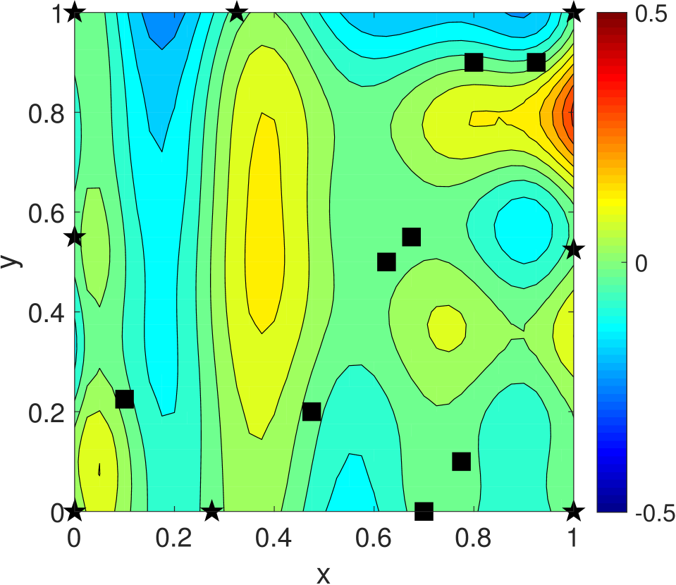
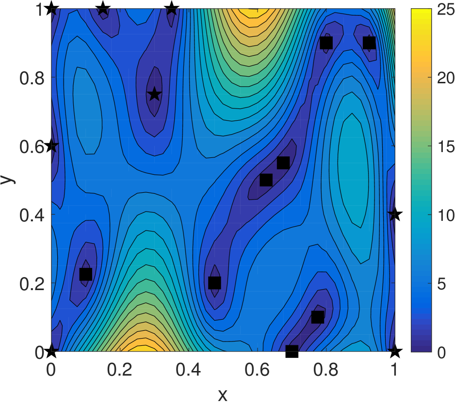
The contours of f𝑓f, together with eight randomly chosen observation locations are presented in Figure 2. The function f𝑓f is evaluated on 41×41414141\times 41 uniform grids, so that the resulting discrete field 𝐅𝐅\mathbf{F} is a 41×41414141\times 41 matrix.

Refer to caption
Figure 2: Contours of modified Branin function (on 41×41414141\times 41 uniform grids) and locations of eight observations (black squares).

In this example, the stochastic model u(𝒙;ω):𝔻×Ω:𝑢𝒙𝜔𝔻Ωu(\bm{x};\omega):\mathbb{D}\times\Omega\rightarrow\mathbb{R} is obtained by modifying the second g𝑔g in f𝑓f, and treating the unknown coefficients b𝑏b and q𝑞q in f(𝒙)𝑓𝒙f(\bm{x}) as random fields:

f^(𝒙;ω)=a(y¯b^(𝒙;ω)x¯2+cx¯r)2+g(1p)cos(x¯)+g^+q^(𝒙;ω)x,^𝑓𝒙𝜔𝑎superscript¯𝑦^𝑏𝒙𝜔superscript¯𝑥2𝑐¯𝑥𝑟2𝑔1𝑝¯𝑥^𝑔^𝑞𝒙𝜔𝑥\hat{f}(\bm{x};\omega)=a(\bar{y}-\hat{b}(\bm{x};\omega)\bar{x}^{2}+c\bar{x}-r)^{2}+g(1-p)\cos(\bar{x})+\hat{g}+\hat{q}(\bm{x};\omega)x, (3.2)

where g^=20^𝑔20\hat{g}=20,

b^(𝒙;ω)^𝑏𝒙𝜔\displaystyle\hat{b}(\bm{x};\omega) =b{0.9+0.2πi=13[14i1sin((2i0.5)πx)ξ2i1(ω)+14i+1sin((2i+0.5)πy)ξ2i(ω)]},absent𝑏0.90.2𝜋superscriptsubscript𝑖13delimited-[]14𝑖12𝑖0.5𝜋𝑥subscript𝜉2𝑖1𝜔14𝑖12𝑖0.5𝜋𝑦subscript𝜉2𝑖𝜔\displaystyle=b\left\{0.9+\dfrac{0.2}{\pi}\sum_{i=1}^{3}\left[\dfrac{1}{4i-1}\sin((2i-0.5)\pi x)\xi_{2i-1}(\omega)+\dfrac{1}{4i+1}\sin((2i+0.5)\pi y)\xi_{2i}(\omega)\right]\right\},
q^(𝒙;ω)^𝑞𝒙𝜔\displaystyle\hat{q}(\bm{x};\omega) =q{1.0+0.6πi=13[14i3cos((2i1.5)πx)ξ2i+5(ω)+14i1cos((2i0.5)πy)ξ2i+6(ω)]},absent𝑞1.00.6𝜋superscriptsubscript𝑖13delimited-[]14𝑖32𝑖1.5𝜋𝑥subscript𝜉2𝑖5𝜔14𝑖12𝑖0.5𝜋𝑦subscript𝜉2𝑖6𝜔\displaystyle=q\left\{1.0+\dfrac{0.6}{\pi}\sum_{i=1}^{3}\left[\dfrac{1}{4i-3}\cos((2i-1.5)\pi x)\xi_{2i+5}(\omega)+\dfrac{1}{4i-1}\cos((2i-0.5)\pi y)\xi_{2i+6}(\omega)\right]\right\},

and {ξi(ω)}i=112superscriptsubscriptsubscript𝜉𝑖𝜔𝑖112\{\xi_{i}(\omega)\}_{i=1}^{12} are iid Gaussian random variables with zero mean and unit variance. This stochastic model includes unkown “physics” (b^^𝑏\hat{b} and q^^𝑞\hat{q}) and incorrect “physics” (g^^𝑔\hat{g}). We compute M=300𝑀300M=300 realizations of u(𝒙;ω)𝑢𝒙𝜔u(\bm{x};\omega), denoted as {𝐅^m}m=1Msuperscriptsubscriptsuperscript^𝐅𝑚𝑚1𝑀\{\hat{\mathbf{F}}^{m}\}_{m=1}^{M}, by generating M=300𝑀300M=300 samples of {ξi(ω)}i=112superscriptsubscriptsubscript𝜉𝑖𝜔𝑖112\{\xi_{i}(\omega)\}_{i=1}^{12} and evaluating u(𝒙;ω)𝑢𝒙𝜔u(\bm{x};\omega) on the 41×41414141\times 41 uniform grids for each of them. Of note, function f𝑓f is not a realization of u(𝒙;ω)𝑢𝒙𝜔u(\bm{x};\omega).

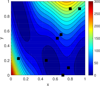
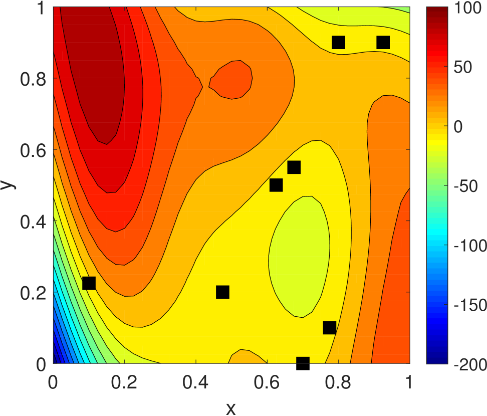
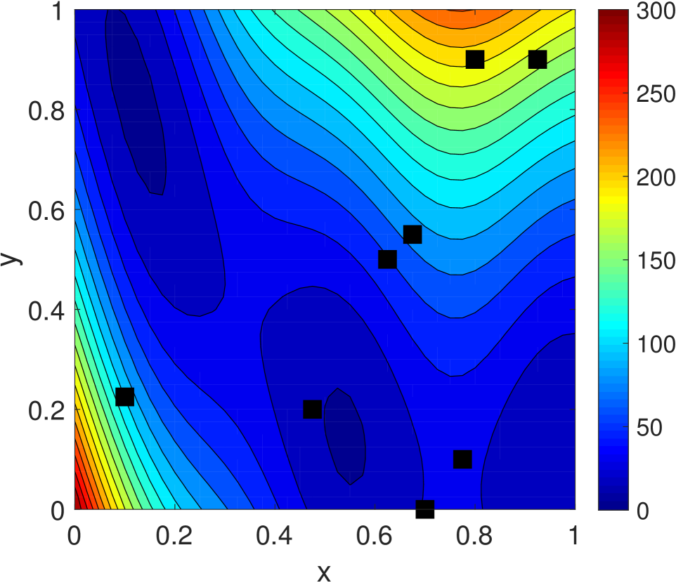
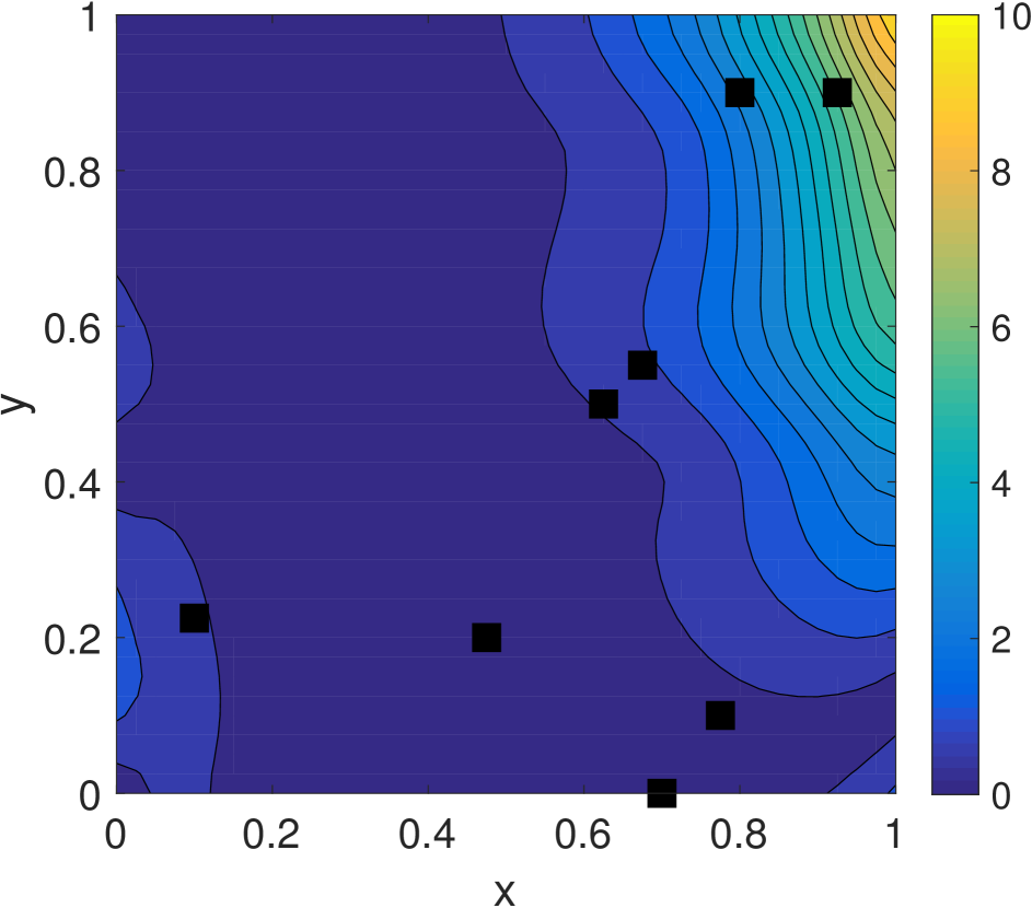
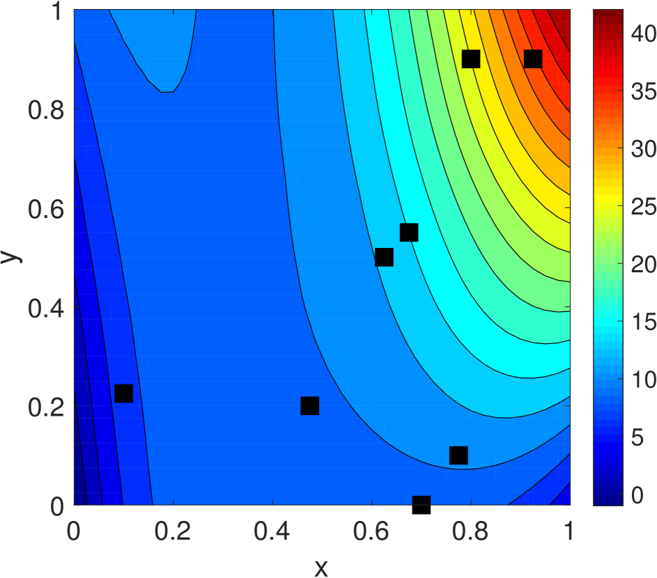
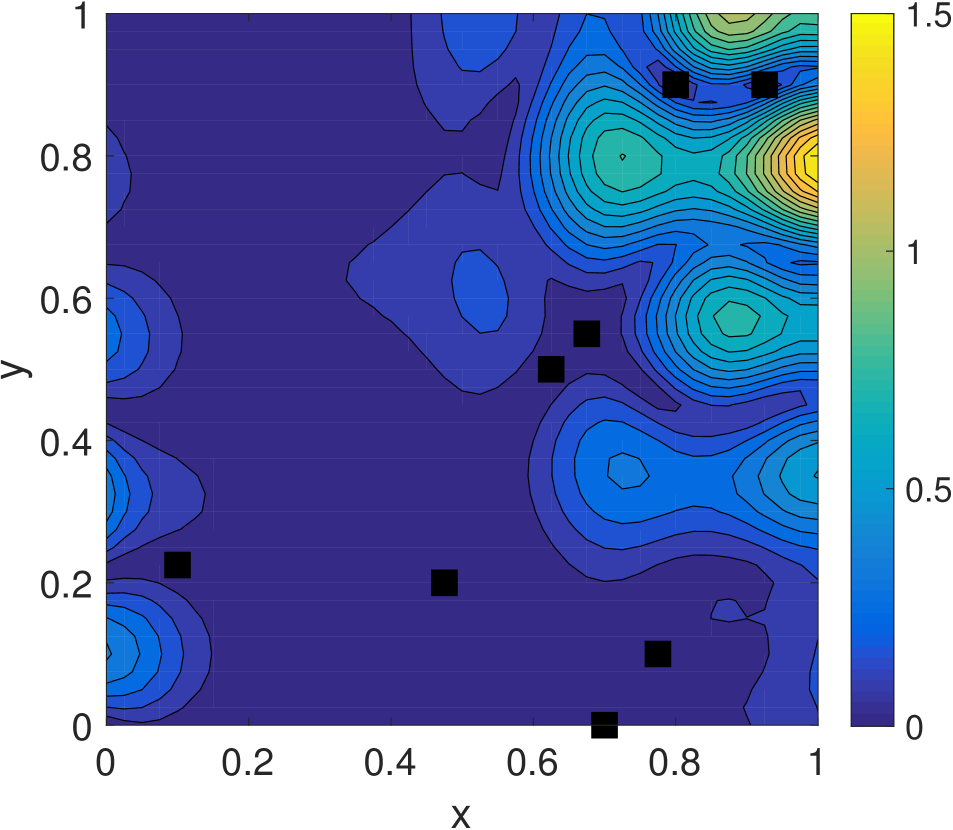
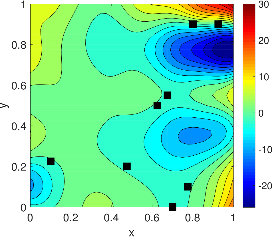
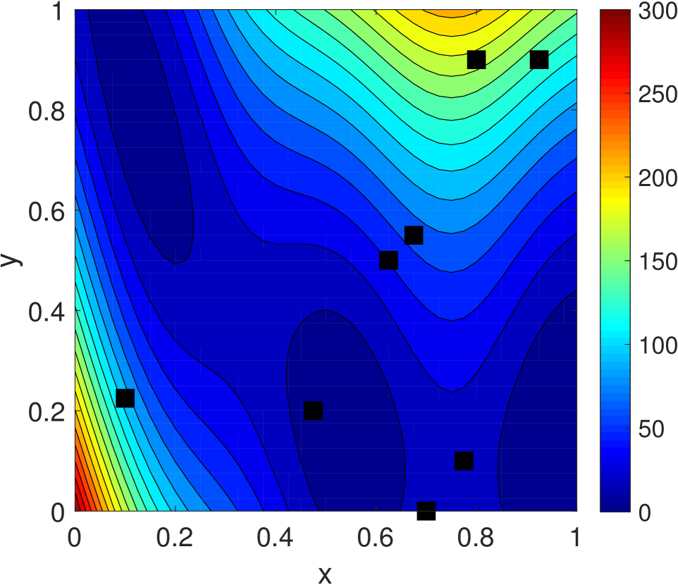
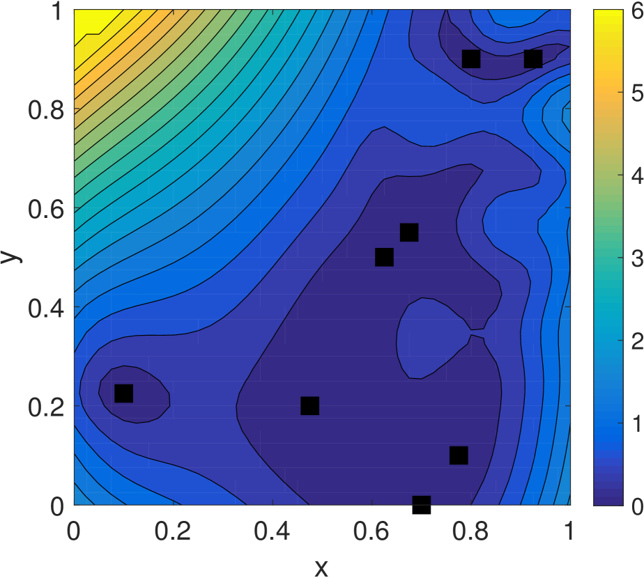
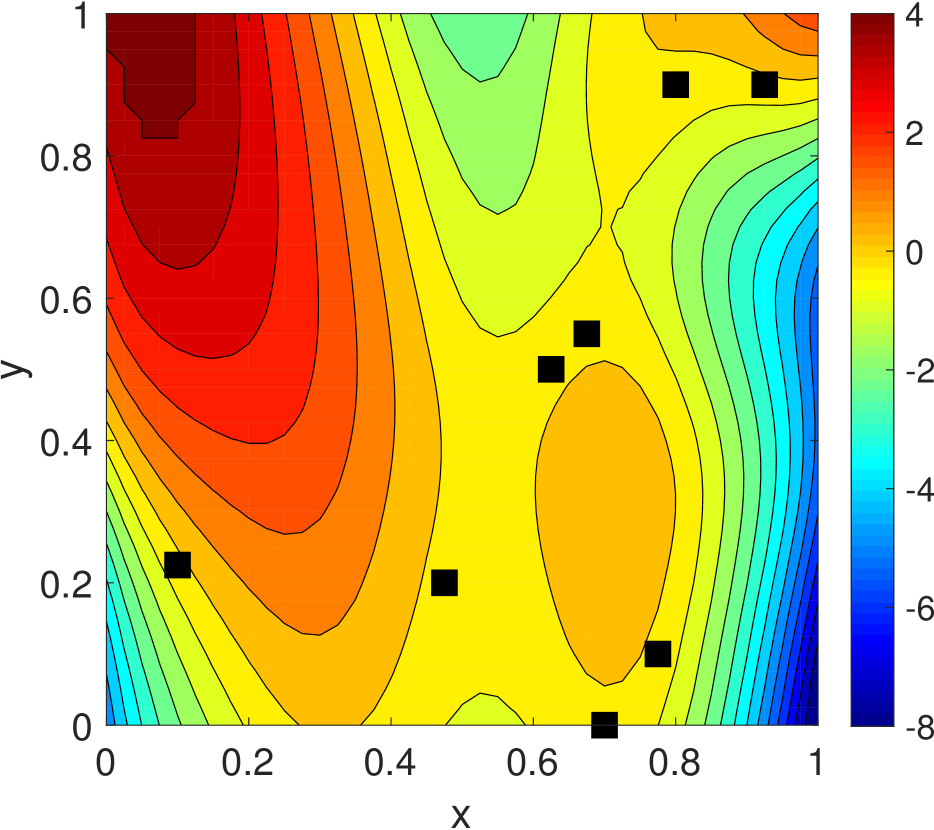
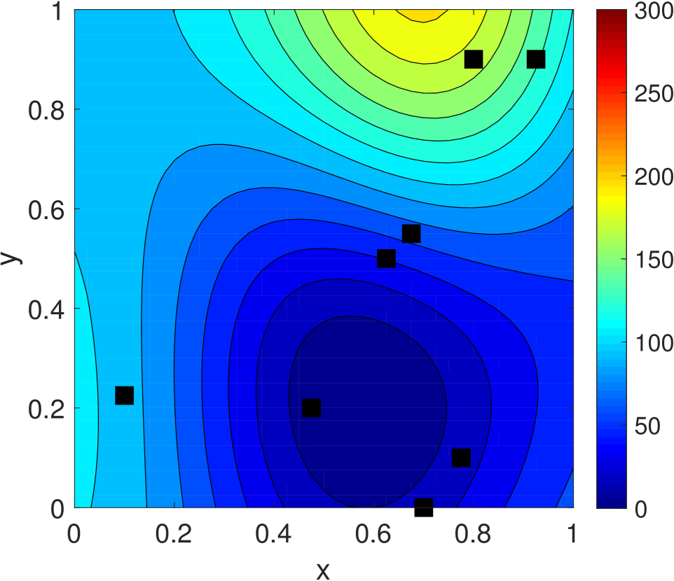
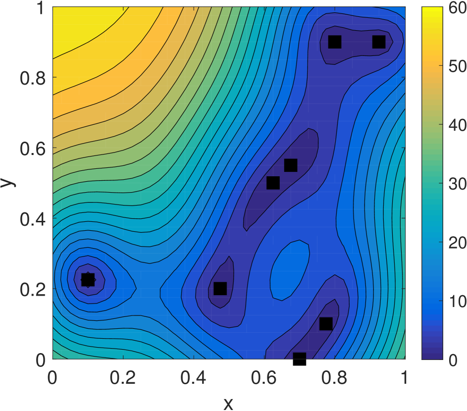
Figure 3 compares the purely data-driven reconstruction (i.e., Kriging) and purely “physics”-based reconstruction (i.e., mean and variance obtained from the stochastic model Eq. (3.2) without conditioning on data). The first row in Figure 3 presents Kriging results obtained using the eight observations shown in Figure 2. The second row shows the ensemble mean (denoted as μ(𝐅^m)𝜇superscript^𝐅𝑚\mu(\hat{\mathbf{F}}^{m})), standard deviation (denoted as σ(𝐅^m)𝜎superscript^𝐅𝑚\sigma(\hat{\mathbf{F}}^{m})) of {𝐅^m}m=1Msuperscriptsubscriptsuperscript^𝐅𝑚𝑚1𝑀\{\hat{\mathbf{F}}^{m}\}_{m=1}^{M}, and μ(𝐅^m)𝐅𝜇superscript^𝐅𝑚𝐅\mu(\hat{\mathbf{F}}^{m})-\mathbf{F}. The relative error is more than 50%percent5050\% for Kriging and 19%percent1919\% for the ensemble mean. In kriging, s^^𝑠\hat{s} is large in the upper left subdomain where no observations are available. On the other hand, the standard deviation of the realizations is large in the upper right region because of the randomness in the “physical” model. Similarly, |𝐅r𝐅|subscript𝐅𝑟𝐅|\mathbf{F}_{r}-\mathbf{F}| is large in the upper left region, while |μ(𝐅^m)𝐅|𝜇superscript^𝐅𝑚𝐅|\mu(\hat{\mathbf{F}}^{m})-\mathbf{F}| is large in the upper right region. These results demonstrate that the data-driven and physics-based methods have significantly different accuracy in reconstructing the entire field and result in different estimates of uncertainty of the reconstruction.
Refer to caption
(a) Kriging 𝐅rsubscript𝐅𝑟\mathbf{F}_{r}
Refer to caption
(b) Kriging s^^𝑠\hat{s}
Refer to caption
(c) Kriging 𝐅r𝐅subscript𝐅𝑟𝐅\mathbf{F}_{r}-\mathbf{F}
Refer to caption
(d) μ(𝐅^m)𝜇superscript^𝐅𝑚\mu(\hat{\mathbf{F}}^{m})
Refer to caption
(e) σ(𝐅^m)𝜎superscript^𝐅𝑚\sigma(\hat{\mathbf{F}}^{m})
Refer to caption
(f) μ(𝐅^m)𝐅𝜇superscript^𝐅𝑚𝐅\mu(\hat{\mathbf{F}}^{m})-\mathbf{F}
Figure 3: Reconstruction of the modified Branin function by Kriging (first row) and statistics of the ensemble {𝐅^m}m=1Msuperscriptsubscriptsuperscript^𝐅𝑚𝑚1𝑀\{\hat{\mathbf{F}}^{m}\}_{m=1}^{M} (second row).

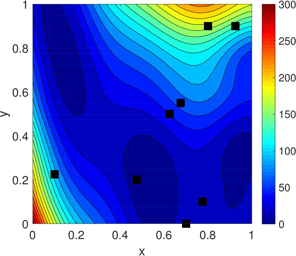
Figure 4 presents results obtained using PhIK and CoPhIK. In this case, CoPhIK outperforms PhIK in the accuracy, and both methods are significantly more accurate than Kriging. However, PhIK shows smaller s^^𝑠\hat{s} than CoPhIK, and s^^𝑠\hat{s} in both PhIK and CoPhIK is significantly smaller than in Kriging. This is because the prior covariance of PhIK is decided by the realizations, and it doesn’t account for the observation. Therefore, the uncertainty of the PhIK result (s^^𝑠\hat{s} of PhIK) is bounded by the uncertainty of the stochastic model (σ(𝑭^m)𝜎superscript^𝑭𝑚\sigma(\hat{\bm{F}}^{m})). Also, the pattern of s^^𝑠\hat{s} in PhIK is similar to that of σ(𝐅^m)𝜎superscript^𝐅𝑚\sigma(\hat{\mathbf{F}}^{m}) in Figure 3(e), i.e., it is large in the right subdomain and small in the left subdomain. On the other hand, CoPhIK incorporates the observation in the posterior mean and kernel as we illustrate in Section 2, and its s^^𝑠\hat{s} pattern is more similar to Kriging’s in Figure 3(b) as we use the Gaussian kernel for both kriging and CoPhIK.
Refer to caption
(a) PhIK 𝐅rsubscript𝐅𝑟\mathbf{F}_{r}
Refer to caption
(b) PhIK s^^𝑠\hat{s}
Refer to caption
(c) PhIK 𝐅r𝐅subscript𝐅𝑟𝐅\mathbf{F}_{r}-\mathbf{F}
Refer to caption
(d) CoPhIK 𝐅rsubscript𝐅𝑟\mathbf{F}_{r}
Refer to caption
(e) CoPhIK s^^𝑠\hat{s}
Refer to caption
(f) CoPhIK 𝐅r𝐅subscript𝐅𝑟𝐅\mathbf{F}_{r}-\mathbf{F}
Figure 4: Reconstruction of the modified Branin function by PhIK (first row) and CoPhIK (second row).

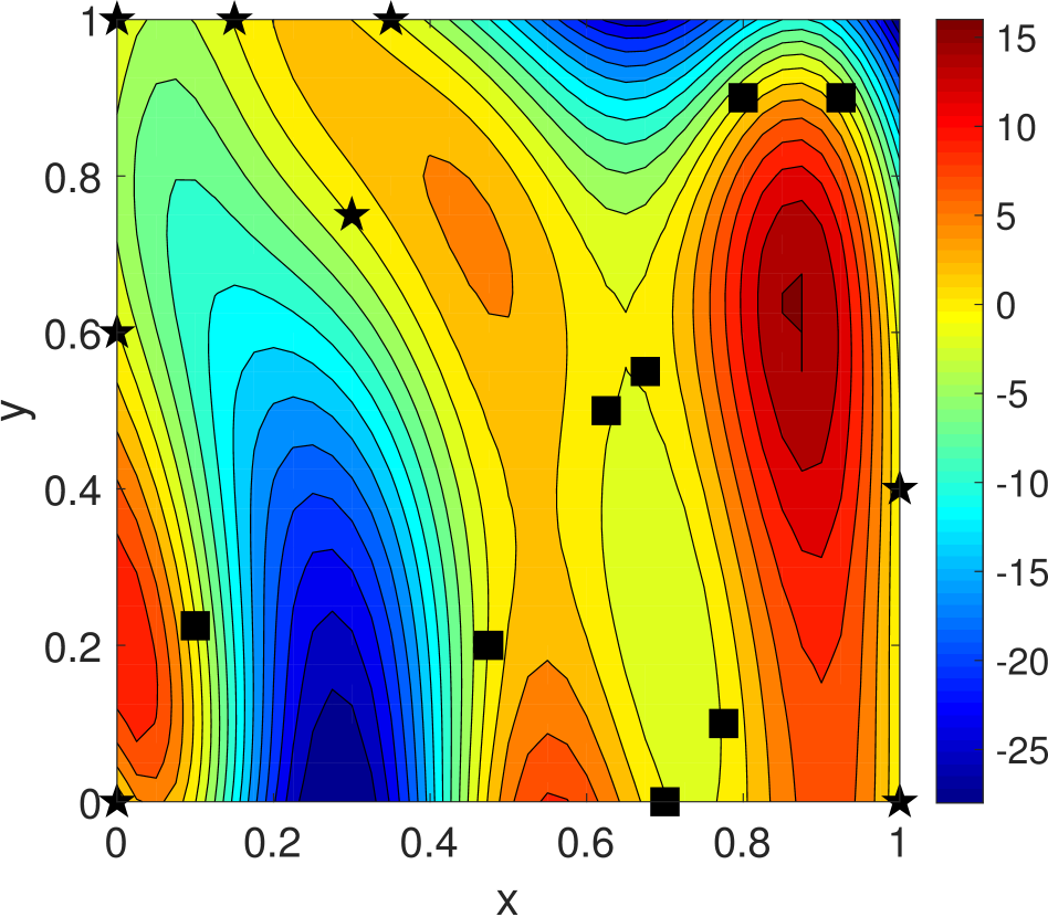
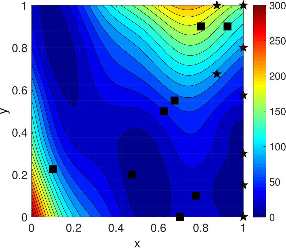
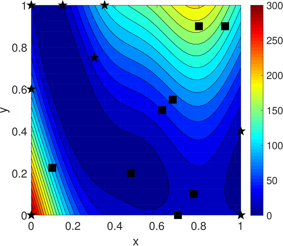
We use Algorithm 2 in combination with kriging, PhIK, and CoPhIK to perform active learning by adding one by one new observations of f𝑓f at the global maximum of s^^𝑠\hat{s}. Figure 5 presents the reconstructions of the modified Branin function with eight new observations added using active learning. In this figure, the first, second and third row corresponds to Kriging, PhIK and CoPhIK, respectively. The initial eight observations are marked by squares, and added observations are marked by stars. By comparing to Figures 3 and 4 it can be seen that reconstruction accuracy increases as more observations are added, and the uncertainty in the reconstruction is reduced. It can also be seen that the additional observation locations identified by CoPhIK are similar to that of kriging. In contrast, most of the additional observations identified by PhIK are on the right boundary.
Refer to caption
(a) Kriging 𝐅rsubscript𝐅𝑟\mathbf{F}_{r}
Refer to caption
(b) Kriging s^^𝑠\hat{s}
Refer to caption
(c) Kriging 𝐅r𝐅subscript𝐅𝑟𝐅\mathbf{F}_{r}-\mathbf{F}
Refer to caption
(d) PhIK 𝐅rsubscript𝐅𝑟\mathbf{F}_{r}
Refer to caption
(e) PhIK s^^𝑠\hat{s}
Refer to caption
(f) PhIK 𝐅r𝐅subscript𝐅𝑟𝐅\mathbf{F}_{r}-\mathbf{F}
Refer to caption
(g) CoPhIK 𝐅rsubscript𝐅𝑟\mathbf{F}_{r}
Refer to caption
(h) CoPhIK s^^𝑠\hat{s}
Refer to caption
(i) CoPhIK 𝐅r𝐅subscript𝐅𝑟𝐅\mathbf{F}_{r}-\mathbf{F}
Figure 5: Reconstruction of the modified Branin function via active learning. Black squares are the locations of the original eight observations. Stars are newly added eight observations based on the actively learning algorithm.

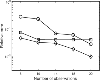
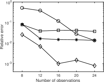
Figure 6 compares the relative error 𝐅r𝐅F/𝐅Fsubscriptnormsubscript𝐅𝑟𝐅𝐹subscriptnorm𝐅𝐹\|\mathbf{F}_{r}-\mathbf{F}\|_{F}/\|\mathbf{F}\|_{F} as a function of the total number of observations for active learning based on kriging, PhIK, modified PhIK and CoPhIK. For the original eight observations, the largest error is in Kriging (over 50%) followed by PhIK and modified PhIK errors (about 8%percent88\%), with the smallest error in CoPhIK (less than 3%percent33\%). As more observations are added by the active learning algorithm, the error of Kriging decreases to approximately 1.5%percent1.51.5\% at 242424 observations. The error of PhIK is reduced from around 8%percent88\% to approximately 4%percent44\% at 121212 observations. Adding 121212 more observations doesn’t improve the accuracy. The error of modified PhIK is reduced from 8%percent88\% to 2%percent22\% at 121212 observations, then it changes very slowly with additional observations. With 242424 observations, the accuracy of Kriging and modified PhIK is approximately the same. CoPhIK has the best accuracy among all the methods and, in general, its error decreases with additional measurements. The error in CoPhIK reduces to less than 0.1%percent0.10.1\% with 242424 observations in total, which is more than one order of magnitude better than the other three methods.
Refer to caption
Figure 6: Relative error of reconstructed modified Branin function 𝑭r𝑭F/𝑭Fsubscriptnormsubscript𝑭𝑟𝑭𝐹subscriptnorm𝑭𝐹\|\bm{F}_{r}-\bm{F}\|_{F}/\|\bm{F}\|_{F} using Kriging (“\circ”), PhIK (“\square”), modified PhIK (“\ast”) and CoPhIK (“\diamond”) with different numbers of total observations via active learning.

Finally, this example also illustrates that smaller uncertainty (s^^𝑠\hat{s}) doesn’t lead to smaller error in the posterior mean. In particular, in this case, PhIK has the smallest s^^𝑠\hat{s}, but CoPhIK posterior mean is the most accurate.

3.2 Heat transfer

In the second example, we consider the steady state of a heat transfer problem. The dimensionless heat equation is given as

Tt(κ(T)T)=0,𝒙𝔻,formulae-sequence𝑇𝑡𝜅𝑇𝑇0𝒙𝔻\dfrac{\partial T}{\partial t}-\nabla\cdot(\kappa(T)\nabla T)=0,\quad\bm{x}\in\mathbb{D}, (3.3)

subject to the boundary conditions:

{T=30cos(2πx)+40,xΓ1,T𝒏=20,xΓ2,T=30cos(2π(x+0.1))+40,xΓ3,T𝒏=20,xΓ4,T𝒏=0,xΓ5.\left\{\begin{aligned} T&=-30\cos(2\pi x)+40,&&x\in\Gamma_{1},\\ \frac{\partial T}{\partial\bm{n}}&=-20,&&x\in\Gamma_{2},\\ T&=30\cos(2\pi(x+0.1))+40,&&x\in\Gamma_{3},\\ \dfrac{\partial T}{\partial\bm{n}}&=20,&&x\in\Gamma_{4},\\ \dfrac{\partial T}{\partial\bm{n}}&=0,&&x\in\Gamma_{5}.\end{aligned}\right. (3.4)

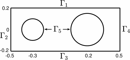
Here, T(𝒙,t)𝑇𝒙𝑡T(\bm{x},t) is the temperature and κ(T)𝜅𝑇\kappa(T) is the temperature-dependent heat conductivity. The computational domain 𝔻𝔻\mathbb{D} is the rectangle [0.5,0.5]×[0.2,0.2]0.50.50.20.2[-0.5,0.5]\times[-0.2,0.2] with two circular cavities R1(O1,r1)subscript𝑅1subscript𝑂1subscript𝑟1R_{1}(O_{1},r_{1}) and R2(O2,r2)subscript𝑅2subscript𝑂2subscript𝑟2R_{2}(O_{2},r_{2}), with O1=(0.3,0),O2=(0.2,0),r1=0.1,r2=0.15formulae-sequencesubscript𝑂10.30formulae-sequencesubscript𝑂20.20formulae-sequencesubscript𝑟10.1subscript𝑟20.15O_{1}=(-0.3,0),O_{2}=(0.2,0),r_{1}=0.1,r_{2}=0.15 (see Figure 7). The reference conductivity is set as

κ(T)=1.0+exp(0.02T),𝜅𝑇1.00.02𝑇\kappa(T)=1.0+\exp(0.02T), (3.5)

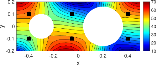
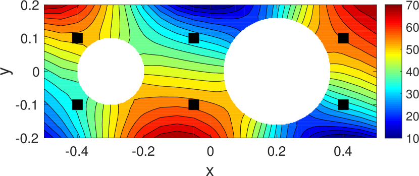
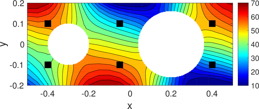
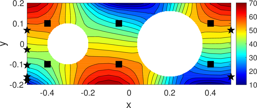
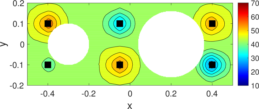
which results in the reference steady state temperature field shown in Figure 8. This solution was obtained by solving Eq. 3.3 and 3.4 using the finite element method with unstructured triangular mesh implemented by the MATLAB PDE toolbox. The number of degrees of freedom is 131913191319, with a maximum grid size of 0.020.020.02. Observations of this exact profile are collected at six locations, marked by black squares in Figure 8.
Refer to caption
Figure 7: Heat transfer solution (steady state) computational domain.
Refer to caption
Figure 8: Contours of heat transfer solution (steady state) and locations of six observations (black squares).

Now we assume that the conductivity model (3.5) is unknown and an “expert knowledge” of κ𝜅\kappa is expressed as

κ(T;ω)=0.1+ξ(ω)T,𝜅𝑇𝜔0.1𝜉𝜔𝑇\kappa(T;\omega)=0.1+\xi(\omega)T, (3.6)

where ξ(ω)𝜉𝜔\xi(\omega) is a uniform random variable 𝒰[0.0012,0.0108]𝒰0.00120.0108\mathcal{U}[0.0012,0.0108]. Note that this example represents a biased expert knowledge that systematically underestimates the heat conductivity and assumes an incorrect functional dependence of κ𝜅\kappa on T𝑇T. We sample the stochastic model by generating M=400𝑀400M=400 samples of ξ(ω)𝜉𝜔\xi(\omega) and then solving Eq. (3.3) for each realization. We denote the resulting ensemble of temperatures solutions by {𝐅^m}m=1Msuperscriptsubscriptsuperscript^𝐅𝑚𝑚1𝑀\{\hat{\mathbf{F}}^{m}\}_{m=1}^{M}.

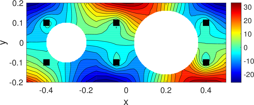
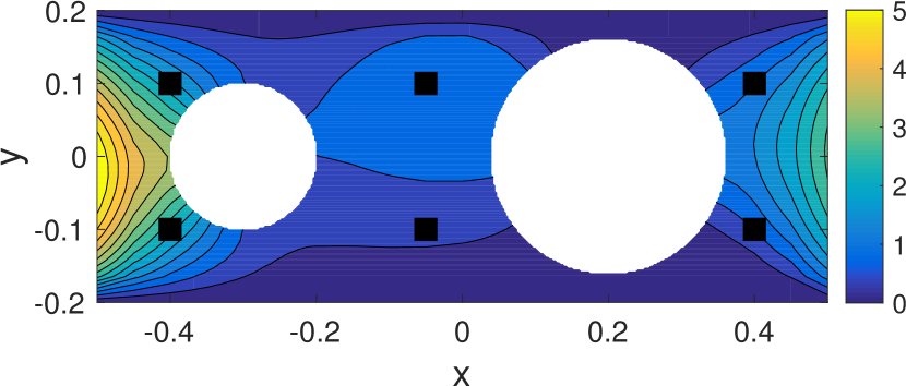
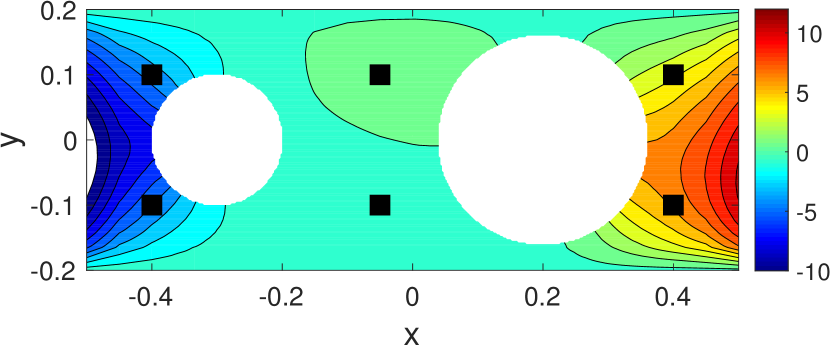
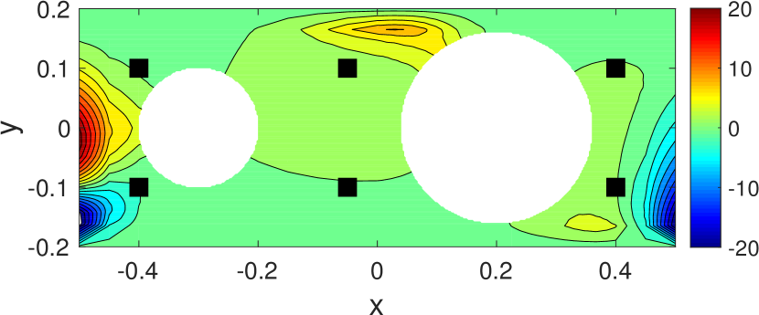
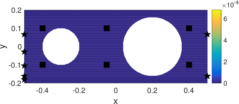
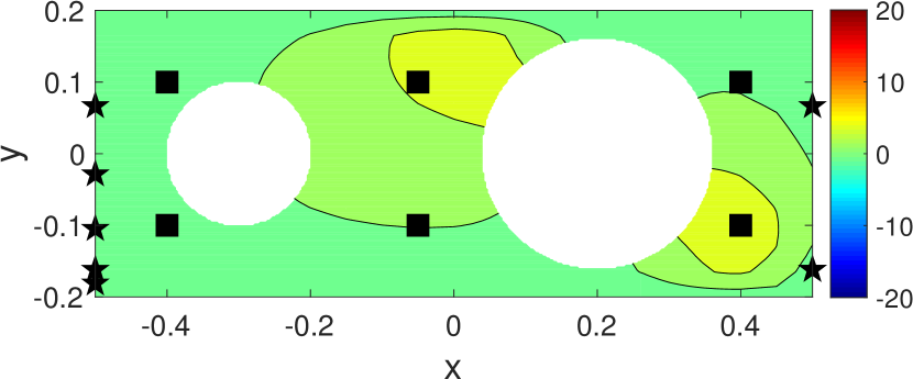
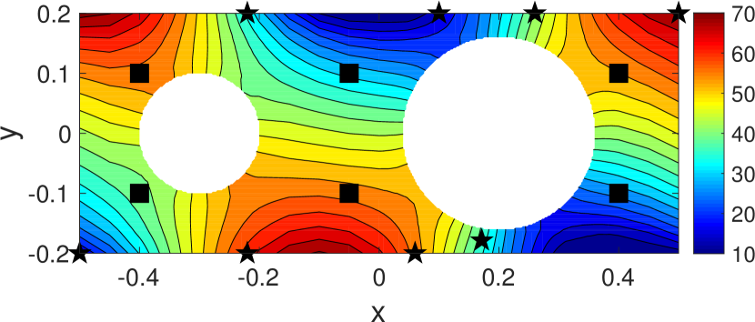
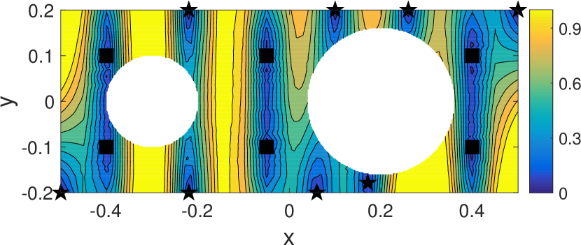
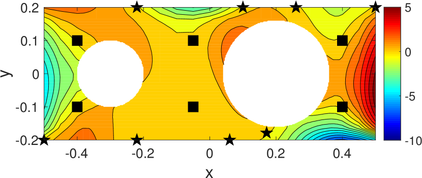
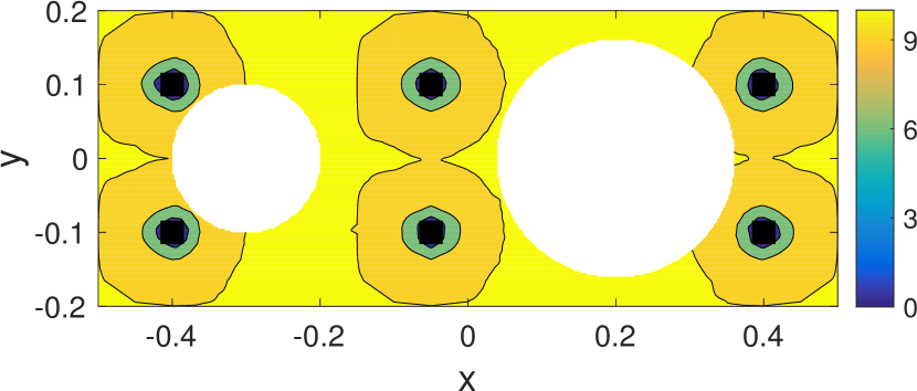
The first row in Figure 9 presents the posterior mean, RMSE and pointwise reconstruction error of Kriging regression obtained with six measurements whose locations are also shown in this figure. The relative error is large (about 27%percent2727\%). The second row in Figure 9 shows the mean and standard deviation of the ensemble {𝐅^}m=1Msuperscriptsubscript^𝐅𝑚1𝑀\{\hat{\mathbf{F}}\}_{m=1}^{M} and the difference between the ensemble mean and the exact field. In this case, the relative error of the ensemble average is 8%percent88\%, which may be acceptable in some application. For the selected number and locations of observations, Kriging performs worse than the unconditional stochastic model.
Refer to caption
(a) Kriging 𝐅rsubscript𝐅𝑟\mathbf{F}_{r}
Refer to caption
(b) Kriging s^^𝑠\hat{s}
Refer to caption
(c) Kriging 𝐅r𝐅subscript𝐅𝑟𝐅\mathbf{F}_{r}-\mathbf{F}
Refer to caption
(d) μ(𝐅^m)𝜇superscript^𝐅𝑚\mu(\hat{\mathbf{F}}^{m})
Refer to caption
(e) σ(𝐅^m)𝜎superscript^𝐅𝑚\sigma(\hat{\mathbf{F}}^{m})
Refer to caption
(f) μ(𝐅^m)𝐅𝜇superscript^𝐅𝑚𝐅\mu(\hat{\mathbf{F}}^{m})-\mathbf{F}
Figure 9: Reconstruction of the steady state solution for heat transfer problem by Kriging (first row) and statistics of the ensemble {𝐅^m}m=1Msuperscriptsubscriptsuperscript^𝐅𝑚𝑚1𝑀\{\hat{\mathbf{F}}^{m}\}_{m=1}^{M} (second row).

Next, we use PhIK and CoPhIK to obtain prediction of T𝑇T. Figure 10 shows the results for PhIK in the top row and for CoPhIK in the bottom row. CoPhIK outperforms PhIK as it results in smaller reconstruction errors. The relative errors of the reconstruction are 4.8%percent4.84.8\% for CoPhIK and 7.8%percent7.87.8\% for PhIK. As before, s^^𝑠\hat{s} in PhIK is smaller than in CoPhIK. Both, PhIK and CoPhIK are more accurate and certain than Kriging.
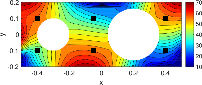
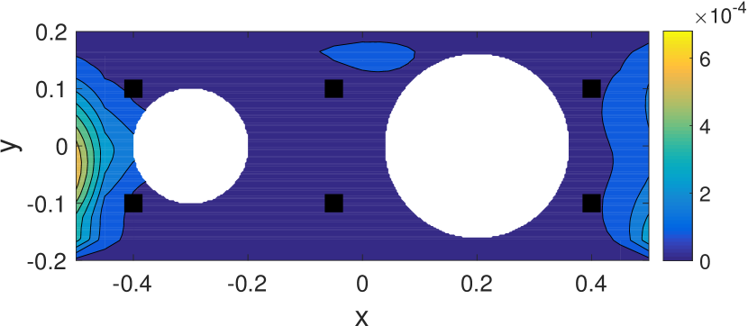
Refer to caption
(a) PhIK 𝑭rsubscript𝑭𝑟\bm{F}_{r}
Refer to caption
(b) PhIK s^^𝑠\hat{s}
Refer to caption
(c) PhIK 𝑭r𝑭subscript𝑭𝑟𝑭\bm{F}_{r}-\bm{F}
Refer to caption
(d) CoPhIK 𝑭rsubscript𝑭𝑟\bm{F}_{r}
Refer to caption
(e) CoPhIK s^^𝑠\hat{s}
Refer to caption
(f) CoPhIK 𝑭r𝑭subscript𝑭𝑟𝑭\bm{F}_{r}-\bm{F}
Figure 10: Reconstruction of the steady state solution for heat transfer problem by PhIK (first row) and CoPhIK (second row).

Finally, we employ active learning to identify additional observation locations. Figure 11 displays Kriging, PhIK, and CoPhIK predictions obtained with 141414 observations. Eight new observations are marked with stars and original six observations are denoted with squares. These three methods place additional observations at different locations. Kriging suggests new observation locations mostly along the external boundaries as there are no original observations on the boundaries and extrapolation in Kriging is the most uncertain in these subdomains. PhIK identifies additional observation on the Neumann boundaries Γ2subscriptΓ2\Gamma_{2} and Γ4subscriptΓ4\Gamma_{4}. CoPhIK identifies new observations locations on boundaries in a manner similar to Kriging, but also adds an observation location in the interior of 𝔻𝔻\mathbb{D}. Figure 12 presents a quantitative study of the relative error as a function of the total number of observations for the three methods. It shows that CoPhIK is more accurate than Kriging and PhIK for a given number of observation points. As more observations are available, the errors in Kriging and CoPhIK decrease while the error of PhIK reaches a constant value after the first few observations. In this case, when 222222 observations are used (six original ones plus 141414 added ones through active learning), the relative errors are 3%percent33\%, 4%percent44\%, and less than 1%percent11\% for Kriging, PhIK and CoPhIK, respectively. We also used the modified PhIK method to model the data and found that the relative error in this method is slightly smaller than in PhIK. However, the modified PhIK reconstruction does not satisfy the Dirichlet boundary condition on Γ1subscriptΓ1\Gamma_{1} and Γ3subscriptΓ3\Gamma_{3}. Therefore, we do not report the modified PhIK results.
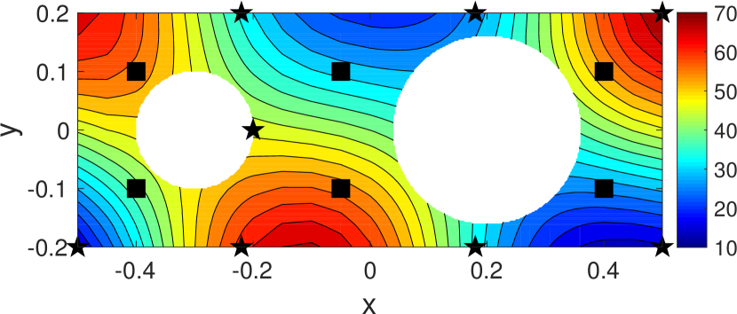
Refer to caption
(a) Kriging 𝐅rsubscript𝐅𝑟\mathbf{F}_{r}
Refer to caption
(b) Kriging s^^𝑠\hat{s}
Refer to caption
(c) Kriging 𝐅r𝐅subscript𝐅𝑟𝐅\mathbf{F}_{r}-\mathbf{F}
Refer to caption
(d) PhIK 𝐅rsubscript𝐅𝑟\mathbf{F}_{r}
Refer to caption
(e) PhIK s^^𝑠\hat{s}
Refer to caption
(f) PhIK 𝐅r𝐅subscript𝐅𝑟𝐅\mathbf{F}_{r}-\mathbf{F}
Refer to caption
(g) CoPhIK 𝐅rsubscript𝐅𝑟\mathbf{F}_{r}
Refer to caption
(h) CoPhIK s^^𝑠\hat{s}
Refer to caption
(i) CoPhIK 𝐅r𝐅subscript𝐅𝑟𝐅\mathbf{F}_{r}-\mathbf{F}
Figure 11: Reconstruction of the heat transfer via active learning. Black squares are the locations of the original six observation. Stars are newly added eight observations based on the actively learning algorithm.
Refer to caption
Figure 12: Relative error of reconstructed steady state solution for heat transfer problem 𝐅r𝐅F/𝐅Fsubscriptnormsubscript𝐅𝑟𝐅𝐹subscriptnorm𝐅𝐹\|\mathbf{F}_{r}-\mathbf{F}\|_{F}/\|\mathbf{F}\|_{F} using Kriging (“\circ”), PhIK (“\square”) and CoPhIK (“\diamond”) with different numbers of total observations via active learning.

3.3 Solute transport in heterogeneous porous media

In this example, we consider conservative transport in a steady-state velocity field in heterogeneous porous media. Let C(𝒙,t)𝐶𝒙𝑡C(\bm{x},t) (𝒙=(x,y)𝒙superscript𝑥𝑦top\bm{x}=(x,y)^{\top}) denote the solute concentration. We assume that measurements of C(𝒙,t)𝐶𝒙𝑡C(\bm{x},t) are available at several locations at different times. The flow and transport processes can be described by conservation laws. In particular, the flow is described by the Darcy flow equation

{(Kh)=0,𝒙𝔻,h𝒏=0,y=0ory=L2,h=H1x=0,h=H2x=L1,cases𝐾0𝒙𝔻𝒏0𝑦0or𝑦subscript𝐿2subscript𝐻1𝑥0subscript𝐻2𝑥subscript𝐿1\begin{cases}\nabla\cdot(K\nabla h)=0,&\bm{x}\in\mathbb{D},\\ \dfrac{\partial h}{\partial\bm{n}}=0,&y=0~{}\text{or}~{}y=L_{2},\\ h=H_{1}&x=0,\\ h=H_{2}&x=L_{1},\end{cases} (3.7)

where h(𝒙;ω)𝒙𝜔h(\bm{x};\omega) is the hydraulic head, 𝔻=[0,L1]×[0,L2]𝔻0subscript𝐿10subscript𝐿2\mathbb{D}=[0,L_{1}]\times[0,L_{2}], L1=256subscript𝐿1256L_{1}=256, L2=128subscript𝐿2128L_{2}=128 is the simulation domain, H1subscript𝐻1H_{1} and H2subscript𝐻2H_{2} are known boundary head values, and K(𝒙)𝐾𝒙K(\bm{x}) is the unknown hydraulic conductivity field. This field is modeled as a random log-normally distributed field K(𝒙;ω)=exp(Z(𝒙;ω))𝐾𝒙𝜔𝑍𝒙𝜔K(\bm{x};\omega)=\exp(Z(\bm{x};\omega)), where Z(𝒙;ω)𝑍𝒙𝜔Z(\bm{x};\omega) is a second-order stationary GP with known exponential covariance function Cov{Z(𝒙),Z(𝒙)}=σZ2exp(|𝒙𝒙|/lz)Cov𝑍𝒙𝑍superscript𝒙subscriptsuperscript𝜎2𝑍𝒙superscript𝒙subscript𝑙𝑧\mathrm{Cov}\{Z(\bm{x}),Z(\bm{x}^{\prime})\}=\sigma^{2}_{Z}\exp(-|\bm{x}-\bm{x}^{\prime}|/l_{z}), variance σZ2=2subscriptsuperscript𝜎2𝑍2\sigma^{2}_{Z}=2, and correlation length lz=5subscript𝑙𝑧5l_{z}=5. The solute transport is governed by the advection-dispersion equation [12, 26]:

{Ct+(𝒗C)=[(Dwτ+𝜶𝒗2)C],𝒙in𝔻,C=Qδ(𝒙𝒙),t=0,C𝒏=0,y=0ory=L2orx=L1,C=0,x=0.cases𝐶𝑡𝒗𝐶delimited-[]subscript𝐷𝑤𝜏𝜶subscriptnorm𝒗2𝐶𝒙in𝔻𝐶𝑄𝛿𝒙superscript𝒙𝑡0𝐶𝒏0𝑦0or𝑦subscript𝐿2or𝑥subscript𝐿1𝐶0𝑥0\begin{cases}\dfrac{\partial C}{\partial t}+\nabla\cdot(\bm{v}C)=\nabla\cdot\left[\left(\dfrac{D_{w}}{\tau}+\bm{\alpha}\|\bm{v}\|_{2}\right)\nabla C\right],&\bm{x}~{}\text{in}~{}\mathbb{D},\\ C=Q\delta(\bm{x}-\bm{x}^{*}),&t=0,\\ \dfrac{\partial C}{\partial\bm{n}}=0,&y=0~{}\text{or}~{}y=L_{2}~{}\text{or}~{}x=L_{1},\\ C=0,&x=0.\end{cases} (3.8)

Here, C(𝒙,t;ω)𝐶𝒙𝑡𝜔C(\bm{x},t;\omega) is the solute concentration defined on 𝔻×[0,T]×Ω𝔻0𝑇Ω\mathbb{D}\times[0,T]\times\Omega; 𝒗𝒗\bm{v} is the fluid velocity given by 𝒗(𝒙;ω)=K(𝒙;ω)h(𝒙;ω)/ϕ𝒗𝒙𝜔𝐾𝒙𝜔𝒙𝜔italic-ϕ\bm{v}(\bm{x};\omega)=-K(\bm{x};\omega)\nabla h(\bm{x};\omega)/\phi, where ϕitalic-ϕ\phi is the porosity; Dwsubscript𝐷𝑤D_{w} is the diffusion coefficient; τ𝜏\tau is the tortuosity; and 𝜶𝜶\bm{\alpha} is the dispersivity tensor with the diagonal components αLsubscript𝛼𝐿\alpha_{L} and αTsubscript𝛼𝑇\alpha_{T}. In the present work, the transport parameters are set to ϕ=0.317italic-ϕ0.317\phi=0.317, τ=ϕ1/3𝜏superscriptitalic-ϕ13\tau=\phi^{1/3}, Dw=2.5×10⁵subscript𝐷𝑤2.5superscript105D_{w}=2.5\times 10^{-5}, αL=5subscript𝛼𝐿5\alpha_{L}=5, and αT=0.5subscript𝛼𝑇0.5\alpha_{T}=0.5. Finally, the solute is instantaneously injected at 𝒙=(50,64)superscript𝒙5064\bm{x}^{*}=(50,64) at t=0𝑡0t=0 with the intensity Q=1𝑄1Q=1.

We are interested in reconstructing the concentration field at T=192𝑇192T=192 (eight days) from sparse observations collected at t=T𝑡𝑇t=T. We generate M𝑀M realizations of Z(𝒙)𝑍𝒙Z(\bm{x}) using the SGSIM (sequential Gaussian simulation) code [11], and solve the governing equations for each realization of K(𝒙)=exp(Z(𝒙))𝐾𝒙𝑍𝒙K(\bm{x})=\exp(Z(\bm{x})) using the finite volume code STOMP (subsurface transport over multiple phases) [47] with grid size 1×1111\times 1. The ground truth Ce(𝒙,T)subscript𝐶𝑒𝒙𝑇C_{e}(\bm{x},T) is randomly selected from the M𝑀M realizations of C(𝒙,T)𝐶𝒙𝑇C(\bm{x},T); this Cesubscript𝐶𝑒C_{e} is excluded from the ensembles used in PhIK or CoPhIK. Figure 13 shows Ce(𝒙,T)subscript𝐶𝑒𝒙𝑇C_{e}(\bm{x},T) with sparse observation locations marked by black squares. We assume that six uniformly spaced observations are available near the boundary of the simulation domain, and nine randomly placed observations are available in the interior of the domain. As Kriging is known to be less accurate for extrapolation, it is a common practice to collect data near the boundary of the domain of interest (e.g., [10]).
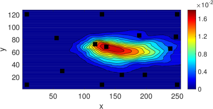
Refer to caption
Figure 13: Ground truth of the solute concentration when T=192𝑇192T=192 and observation locations (black squares).

The first row in Figure 14 shows the reconstruction results obtained using Kriging with Gaussian kernel. The relative error is nearly 50%percent5050\% because a stationary kernel is not capable of resolving the reference field accurately. The second row displays the ensemble mean, standard deviation and the difference of mean and the ground truth, estimated from the stochastic flow and advection-dispersion equation without conditioning on data. Solving these stochastic equations with standard MC requires a large number of simulations. To reduce computational cost of MC, we use MLMC (described in Appendix A) to compute mean and variance of C𝐶C as in [52]. Later, we also use MLMC to compute the covariance of C𝐶C. In MLMC, we use MH=10subscript𝑀𝐻10M_{H}=10 high-resolution simulations (grid size 1×1111\times 1) and ML=150subscript𝑀𝐿150M_{L}=150 low-resolution simulations (grid size 4×4444\times 4). The MLMC mean is almost symmetric which does not reflect the real pattern of the ground truth, which is not symmetric). The relative error of using ensemble mean to estimate the ground truth is 30%percent3030\%. This figure shows that Kriging prediction is less accurate and have larger predictive uncertainty except for the neighborhoods of the observations.
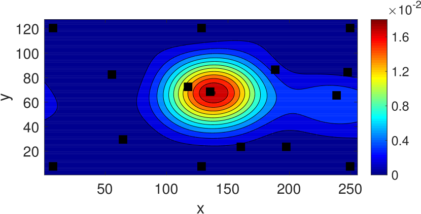
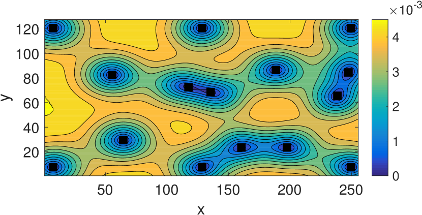
Refer to caption
(a) Kriging 𝐅rsubscript𝐅𝑟\mathbf{F}_{r}
Refer to caption
(b) Kriging s^^𝑠\hat{s}
Refer to caption
(c) Kriging 𝐅r𝐅subscript𝐅𝑟𝐅\mathbf{F}_{r}-\mathbf{F}
Refer to caption
(d) MLMC mean
Refer to caption
(e) MLMC std.
Refer to caption
(f) MLMC mean 𝐅𝐅-\mathbf{F}
Figure 14: Reconstruction of the solute concentration by Kriging (first row) and statistics of MLMC combining the ensemble {𝐅^Lm}m=1MLsuperscriptsubscriptsubscriptsuperscript^𝐅𝑚𝐿𝑚1subscript𝑀𝐿\{\hat{\mathbf{F}}^{m}_{L}\}_{m=1}^{M_{L}} and {𝐅^Hm}m=1MHsuperscriptsubscriptsubscriptsuperscript^𝐅𝑚𝐻𝑚1subscript𝑀𝐻\{\hat{\mathbf{F}}^{m}_{H}\}_{m=1}^{M_{H}} (second row).

Figure 15 shows 𝐅rsubscript𝐅𝑟\mathbf{F}_{r}, s^^𝑠\hat{s}, and 𝐅r𝑭subscript𝐅𝑟𝑭\mathbf{F}_{r}-\bm{F} obtained with PhIK and CoPhIK. In this case, PhIK is more accurate than CoPhiK. The reconstructed field 𝐅rsubscript𝐅𝑟\mathbf{F}_{r} from both methods are closer to the ground truth than the Kriging results, as evident from smaller s^^𝑠\hat{s} and 𝐅r𝑭subscript𝐅𝑟𝑭\mathbf{F}_{r}-\bm{F}.

Refer to caption
(a) PhIK 𝐅rsubscript𝐅𝑟\mathbf{F}_{r}
Refer to caption
(b) PhIK s^^𝑠\hat{s}
Refer to caption
(c) PhIK 𝐅^r𝐅subscript^𝐅𝑟𝐅\hat{\mathbf{F}}_{r}-\mathbf{F}
Refer to caption
(d) CoPhIK 𝐅rsubscript𝐅𝑟\mathbf{F}_{r}
Refer to caption
(e) CoPhIK s^^𝑠\hat{s}
Refer to caption
(f) CoPhIK 𝐅^r𝐅subscript^𝐅𝑟𝐅\hat{\mathbf{F}}_{r}-\mathbf{F}
Figure 15: Reconstruction of the solute concentration field using PhIK (first row) and CoPhIK (second row).

Finally, we employ the active learning algorithm 2 to identify additional observation locations. Figure 16 presents 151515 additional observation locations, indicated by black stars, identified using Kriging, PhIK and CoPhIK, and the resulting field reconstructions. Both PhIK and CoPhIK outperforms Kriging, which can be seen qualitatively in terms of the structure of the reconstructed plume and quantitative from the pointwise difference 𝐅r𝐅subscript𝐅𝑟𝐅\mathbf{F}_{r}-\mathbf{F}. It can be seen that the additional observations identified by PhIK cluster around the plume, where the concentration is high, while Kriging distributes additional observations more uniformly throughout the entire simulation domain. The behavior of CoPhIK is between that of Kriging and PhIK, placing additional observations around the plume less tightly than PhIK but less spread out than Kriging.
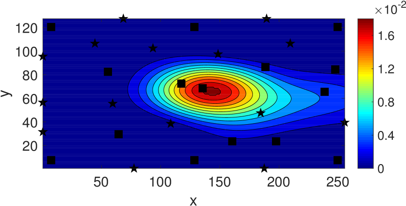
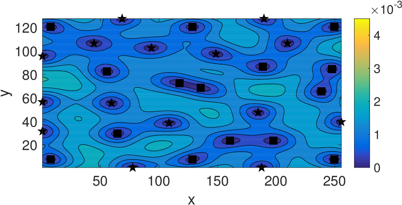
Refer to caption
(a) Kriging 𝐅rsubscript𝐅𝑟\mathbf{F}_{r}
Refer to caption
(b) Kriging s^^𝑠\hat{s}
Refer to caption
(c) Kriging 𝐅r𝐅subscript𝐅𝑟𝐅\mathbf{F}_{r}-\mathbf{F}
Refer to caption
(d) PhIK 𝐅rsubscript𝐅𝑟\mathbf{F}_{r}
Refer to caption
(e) PhIK s^^𝑠\hat{s}
Refer to caption
(f) PhIK 𝐅r𝐅subscript𝐅𝑟𝐅\mathbf{F}_{r}-\mathbf{F}
Refer to caption
(g) CoPhIK 𝐅rsubscript𝐅𝑟\mathbf{F}_{r}
Refer to caption
(h) CoPhIK s^^𝑠\hat{s}
Refer to caption
(i) CoPhIK 𝐅r𝐅subscript𝐅𝑟𝐅\mathbf{F}_{r}-\mathbf{F}
Figure 16: Reconstruction of the solute concentration field via active learning using Kriging (first row), PhIK (second row) and CoPhIK (third row). Black squares are the locations of the original 151515 observation. Stars are 151515 newly added observations.

Figure 17 presents the relative error as a function of the number of additional observation locations identified via active learning. It can be seen that PhIK is more accurate than CoPhIK, especially when number of observations is small. The difference between these two methods becomes smaller as more observations are introduced. The error of Kriging decreases in general with increasing number of observations, but is much larger than that of PhIK and CoPhIK. For modified PhIK, the magnitude of ΔμΔ𝜇\Delta\mu is 𝒪(106)𝒪superscript106\mathcal{O}(10^{-6}), so that its behavior is similar to that of PhIK.
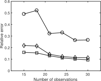
Refer to caption
Figure 17: Relative error of reconstructed solute concentration 𝐅r𝐅F/𝐅Fsubscriptnormsubscript𝐅𝑟𝐅𝐹subscriptnorm𝐅𝐹\|\mathbf{F}_{r}-\mathbf{F}\|_{F}/\|\mathbf{F}\|_{F} of Kriging (“\circ”), PhIK (“\square”) and CoPhIK (“\diamond”) using different numbers of total observations via active learning.

This example is different from the previous two in that a stationary kernel is not suitable for reconstructing the reference solute concentration field. Similarly, a stationary kernel is not adequate for modeling the GP Ydsubscript𝑌𝑑Y_{d} in CoPhIK. In addition, in this case PhIK outperforms CoPhIK because the ground truth is a realization of the stochastic model, i.e., the stochastic model in this case is accurate. This is different from the previous two examples where we use incorrect stochastic physical models. A carefully chosen non-stationary kernel function would be necessary to improve the accuracy of Kriging and CoPhIK.

4 Conclusion

In this work, we propose CoPhIK, a CoKriging-based multifidelity method that uses the PhIK method to combine numerical simulations of physical systems with accurate observations. The CoPhIK method first constructs a “low-fidelity” GP YLsubscript𝑌𝐿Y_{{}_{L}} via PhIK by estimating its mean and covariance function from the output of a stochastic physical model reflecting partial knowledge of the system; then, it models the discrepancy between high-fidelity data (e.g., observations of the system) and the low-fidelity GP using auxiliary GP Ydsubscript𝑌𝑑Y_{{}_{d}}. Whereas in PhIK the (prior) mean and covariance function are entirely defined by the stochastic model outputs, CoPhIK incorporates high-fidelity data in constructing the prior mean and covariance. In addition, we propose a modified version of PhIK by introducing a correction term to the prior mean. We also provide upper bounds for the error in enforcing physical constraints using CoPhIK and modified PhIK. Finally, we demonstrate that an active learning algorithm in combination with Kriging, PhIK and CoPhIK suggests very different locations for new observations, and the two physics-informed methods result in significantly more accurate predictions with reduced uncertainty.

The CoPhIK method presented in this work consists of a non-stationary part YLsubscript𝑌𝐿Y_{{}_{L}}, and a stationary part Ydsubscript𝑌𝑑Y_{{}_{d}}, in contrast with the “data-driven” Kriging method, for which the prior mean and covariance are estimated from data only, usually requiring an assumption of stationarity. The accuracy of CoPhIK predictions and of enforcing physical constraints depends both on the accuracy of the physical model and the selection of the kernel for Ydsubscript𝑌𝑑Y_{{}_{d}}. One can further improve CoPhIK by employing a non-stationary model for Ydsubscript𝑌𝑑Y_{{}_{d}}, thus rendering the GP YHsubscript𝑌𝐻Y_{{}_{H}} fully non-stationary. The choice of non-stationary kernel for Ydsubscript𝑌𝑑Y_{{}_{d}} is problem dependent, and it may be achieved by exploiting additional physical information whenever available.

The presented physics-informed methods are nonintrusive, and can utilize existing domain codes to compute the necessary ensembles. Therefore, these methods are suitable for large-scale complex applications for which physical models and codes are available.

Acknowledgments

We thank Dr. Nathan Baker for fruitful discussion. This work was supported by the U.S. Department of Energy (DOE), Office of Science, Office of Advanced Scientific Computing Research (ASCR) as part of the Uncertainty Quantification in Advection-Diffusion-Reaction Systems. A portion of the research described in this paper was conducted under the Laboratory Directed Research and Development Program at Pacific Northwest National Laboratory (PNNL). PNNL is operated by Battelle for the DOE under Contract DE-AC05-76RL01830.

Appendices

A. Constructing GP Y(𝒙)𝑌𝒙Y(\bm{x}) in PhIK using MLMC

For simplicity, we demonstrate the idea via two-level MLMC [52]. We use uLm(𝒙)superscriptsubscript𝑢𝐿𝑚𝒙u_{{}_{L}}^{m}(\bm{x}) (m=1,,ML𝑚1subscript𝑀𝐿m=1,...,M_{L}) and uHm(𝒙)superscriptsubscript𝑢𝐻𝑚𝒙u_{{}_{H}}^{m}(\bm{x}) (m=1,,MH𝑚1subscript𝑀𝐻m=1,...,M_{H}) to denote MLsubscript𝑀𝐿M_{L} low-accuracy and MHsubscript𝑀𝐻M_{H} high-accuracy realizations of the stochastic model u(𝒙;ω)𝑢𝒙𝜔u(\bm{x};\omega) for the system. In this work, uLmsuperscriptsubscript𝑢𝐿𝑚u_{{}_{L}}^{m} are simulation results on coarse grids 𝔻Lsubscript𝔻𝐿\mathbb{D}_{L}, and uHmsuperscriptsubscript𝑢𝐻𝑚u_{{}_{H}}^{m} are simulations results on fine grids 𝔻Hsubscript𝔻𝐻\mathbb{D}_{H}. We denote u¯(𝒙)=uH(𝒙)uL(𝒙)¯𝑢𝒙subscript𝑢𝐻𝒙subscript𝑢𝐿𝒙\overline{u}(\bm{x})=u_{{}_{H}}(\bm{x})-u_{{}_{L}}(\bm{x}). Here, when computing u¯¯𝑢\overline{u}, we interpolate uLsubscript𝑢𝐿u_{L} from 𝔻Lsubscript𝔻𝐿\mathbb{D}_{L} to 𝔻Hsubscript𝔻𝐻\mathbb{D}_{H}. The mean of Y(𝒙)𝑌𝒙Y(\bm{x}) is estimated as

𝔼{Y(𝒙)}=μ(𝒙)μMLMC(𝒙)=1MLm=1MLuLm(𝒙)+1MHm=1MHu¯m(𝒙).𝔼𝑌𝒙𝜇𝒙subscript𝜇MLMC𝒙1subscript𝑀𝐿superscriptsubscript𝑚1subscript𝑀𝐿superscriptsubscript𝑢𝐿𝑚𝒙1subscript𝑀𝐻superscriptsubscript𝑚1subscript𝑀𝐻superscript¯𝑢𝑚𝒙\mathbb{E}\left\{Y(\bm{x})\right\}=\mu(\bm{x})\approx\mu_{{}_{\mathrm{MLMC}}}(\bm{x})=\dfrac{1}{M_{L}}\sum_{m=1}^{M_{L}}u_{{}_{L}}^{m}(\bm{x})+\dfrac{1}{M_{H}}\sum_{m=1}^{M_{H}}\overline{u}^{m}(\bm{x}). (A.1)

which is the standard MLMC estimate of the mean [17]. The covariance function of Y(𝒙)𝑌𝒙Y(\bm{x}) is estimated as:

Cov{Y(𝒙),Y(𝒙)}kMLMC(𝒙,𝒙)Cov𝑌𝒙𝑌superscript𝒙subscript𝑘MLMC𝒙superscript𝒙\displaystyle\mathrm{Cov}\left\{Y(\bm{x}),Y(\bm{x}^{\prime})\right\}\approx k_{{}_{\mathrm{MLMC}}}(\bm{x},\bm{x}^{\prime}) (A.2)
=\displaystyle= 1ML1m=1ML(uLm(𝒙)1MLm=1MLuLm(𝒙))(uLm(𝒙)1MLm=1MLuLm(𝒙))1subscript𝑀𝐿1superscriptsubscript𝑚1subscript𝑀𝐿superscriptsubscript𝑢𝐿𝑚𝒙1subscript𝑀𝐿superscriptsubscript𝑚1subscript𝑀𝐿superscriptsubscript𝑢𝐿𝑚𝒙superscriptsubscript𝑢𝐿𝑚superscript𝒙1subscript𝑀𝐿superscriptsubscript𝑚1subscript𝑀𝐿superscriptsubscript𝑢𝐿𝑚superscript𝒙\displaystyle\dfrac{1}{M_{L}-1}\sum_{m=1}^{M_{L}}\bigg{(}u_{{}_{L}}^{m}(\bm{x})-\dfrac{1}{M_{L}}\sum_{m=1}^{M_{L}}u_{{}_{L}}^{m}(\bm{x})\bigg{)}\bigg{(}u_{{}_{L}}^{m}(\bm{x}^{\prime})-\dfrac{1}{M_{L}}\sum_{m=1}^{M_{L}}u_{{}_{L}}^{m}(\bm{x}^{\prime})\bigg{)}
+1MH1m=1MH(u¯m(𝒙)1MHm=1MHu¯m(𝒙))(u¯m(𝒙)1MHm=1MHu¯m(𝒙)).1subscript𝑀𝐻1superscriptsubscript𝑚1subscript𝑀𝐻superscript¯𝑢𝑚𝒙1subscript𝑀𝐻superscriptsubscript𝑚1subscript𝑀𝐻superscript¯𝑢𝑚𝒙superscript¯𝑢𝑚superscript𝒙1subscript𝑀𝐻superscriptsubscript𝑚1subscript𝑀𝐻superscript¯𝑢𝑚superscript𝒙\displaystyle+\dfrac{1}{M_{H}-1}\sum_{m=1}^{M_{H}}\bigg{(}\overline{u}^{m}(\bm{x})-\dfrac{1}{M_{H}}\sum_{m=1}^{M_{H}}\overline{u}^{m}(\bm{x})\bigg{)}\bigg{(}\overline{u}^{m}(\bm{x}^{\prime})-\dfrac{1}{M_{H}}\sum_{m=1}^{M_{H}}\overline{u}^{m}(\bm{x}^{\prime})\bigg{)}.

Finally, the MLMC-based PhIK model takes the form

y^(𝒙)=μMLMC(𝒙)+𝒄MLMC𝐂MLMC1(𝒚𝝁MLMC),^𝑦superscript𝒙subscript𝜇MLMCsuperscript𝒙superscriptsubscript𝒄MLMCtopsuperscriptsubscript𝐂MLMC1𝒚subscript𝝁MLMC\hat{y}(\bm{x}^{*})=\mu_{{}_{\mathrm{MLMC}}}(\bm{x}^{*})+\bm{c}_{{}_{\mathrm{MLMC}}}^{\top}\mathbf{C}_{{}_{\mathrm{MLMC}}}^{-1}(\bm{y}-\bm{\mu}_{{}_{\mathrm{MLMC}}}), (A.3)

where 𝝁MLMC=(μMLMC(𝒙(1)),,μMLMC(𝒙(N)))subscript𝝁MLMCsuperscriptsubscript𝜇MLMCsuperscript𝒙1subscript𝜇MLMCsuperscript𝒙𝑁top\bm{\mu}_{{}_{\mathrm{MLMC}}}=\left(\mu_{{}_{\mathrm{MLMC}}}(\bm{x}^{(1)}),\dotsc,\mu_{{}_{\mathrm{MLMC}}}(\bm{x}^{(N)})\right)^{\top}. The matrix 𝐂MLMCsubscript𝐂MLMC\mathbf{C}_{{}_{\mathrm{MLMC}}} and vector 𝒄MLMCsubscript𝒄MLMC\bm{c}_{{}_{\mathrm{MLMC}}} are approximations of 𝐂𝐂\mathbf{C} in Eq. (2.4) and 𝒄𝒄\bm{c} in Eq. (2.8) using kMLMCsubscript𝑘MLMCk_{{}_{\mathrm{MLMC}}} in Eq. (A.2). The MSE of this prediction is

s^2(𝒙)=σMLMC2(𝒙)𝒄MLMC𝐂MLMC1𝒄MLMC,superscript^𝑠2superscript𝒙subscriptsuperscript𝜎2MLMCsuperscript𝒙superscriptsubscript𝒄MLMCtopsuperscriptsubscript𝐂MLMC1subscript𝒄MLMC\hat{s}^{2}(\bm{x}^{*})=\sigma^{2}_{{}_{\mathrm{MLMC}}}(\bm{x}^{*})-\bm{c}_{{}_{\mathrm{MLMC}}}^{\top}\mathbf{C}_{{}_{\mathrm{MLMC}}}^{-1}\bm{c}_{{}_{\mathrm{MLMC}}}, (A.4)

where σMLMC2(𝒙)=kMLMC(𝒙,𝒙)superscriptsubscript𝜎MLMC2superscript𝒙subscript𝑘MLMCsuperscript𝒙superscript𝒙\sigma_{{}_{\mathrm{MLMC}}}^{2}(\bm{x}^{*})=k_{{}_{\mathrm{MLMC}}}(\bm{x}^{*},\bm{x}^{*}). If i.i.d. Gaussian noise is assumed in the observation, replace 𝐂MLMCsubscript𝐂MLMC\mathbf{C}_{{}_{\mathrm{MLMC}}} with 𝐂MLMC+δ2𝐈subscript𝐂MLMCsuperscript𝛿2𝐈\mathbf{C}_{{}_{\mathrm{MLMC}}}+\delta^{2}\mathbf{I}, where δ2superscript𝛿2\delta^{2} is the variance of the noise.

B. Active learning

In this work, active learning is a process of identifying locations for additional observations that minimize the prediction error and reduce MSE or uncertainty, e.g., [8, 19, 46, 9]. We use a greedy algorithm to add additional observations, i.e., to add new observations at the maxima of s(𝒙)𝑠𝒙s(\bm{x}), e.g., [14, 38]. Then, we can make a new prediction y^(𝒙)^𝑦𝒙\hat{y}(\bm{x}) for 𝒙𝔻𝒙𝔻\bm{x}\in\mathbb{D} and compute a new s^2(𝒙)superscript^𝑠2𝒙\hat{s}^{2}(\bm{x}) to select the next location for additional observation (see Algorithm 2).

Algorithm 2 Active learning based on GPR
1:Specify the locations 𝑿𝑿\bm{X}, corresponding observations 𝒚𝒚\bm{y}, and the maximum number of observations Nmaxsubscript𝑁N_{\max} affordable. The number of available observations is denoted as N𝑁N.
2:while Nmax>Nsubscript𝑁𝑁N_{\max}>N do
3:     Compute the MSE s^2(𝒙)superscript^𝑠2𝒙\hat{s}^{2}(\bm{x}) of MLE prediction y^(𝒙)^𝑦𝒙\hat{y}(\bm{x}) for 𝒙𝔻𝒙𝔻\bm{x}\in\mathbb{D}.
4:     Locate the location 𝒙msubscript𝒙𝑚\bm{x}_{m} for the maximum of s^2(𝒙)superscript^𝑠2𝒙\hat{s}^{2}(\bm{x}) for 𝒙𝔻𝒙𝔻\bm{x}\in\mathbb{D}.
5:     Obtain observation ymsubscript𝑦𝑚y_{m} at 𝒙msubscript𝒙𝑚\bm{x}_{m} and set 𝑿={𝑿,𝒙m},𝒚=(𝒚,ym),N=N+1formulae-sequence𝑿𝑿subscript𝒙𝑚formulae-sequence𝒚superscriptsuperscript𝒚topsubscript𝑦𝑚top𝑁𝑁1\bm{X}=\{\bm{X},\bm{x}_{m}\},\bm{y}=(\bm{y}^{\top},y_{m})^{\top},N=N+1.
6:end while
7:Construct the MLE prediction of y^(𝒙)^𝑦𝒙\hat{y}(\bm{x}) on 𝔻𝔻\mathbb{D} using 𝑿𝑿\bm{X} and 𝒚𝒚\bm{y}.

This selection criterion is based on the statistical interpretation of the interpolation. More sophisticated sensor placement algorithms can be found in literature, e.g., [19, 23, 16], and PhIK or CoPhIK are complementary to these methods.

References

  • [1] Margaret Armstrong. Problems with universal kriging. Journal of the International Association for Mathematical Geology, 16(1):101–108, 1984.
  • [2] David A Barajas-Solano and Alexandre M Tartakovsky. Multivariate gaussian process regression for multiscale data assimilation and uncertainty reduction. arXiv preprint arXiv:1804.06490, 2018.
  • [3] David A. Barajas-Solano and Alexandre M. Tartakovsky. Probability and cumulative density function methods for the stochastic advection-reaction equation. SIAM/ASA Journal on Uncertainty Quantification, 6(1):180–212, 2018.
  • [4] Sofiane Brahim-Belhouari and Amine Bermak. Gaussian process for nonstationary time series prediction. Computational Statistics & Data Analysis, 47(4):705–712, 2004.
  • [5] Christopher James Brooks, AIJ Forrester, AJ Keane, and S Shahpar. Multi-fidelity design optimisation of a transonic compressor rotor. 2011.
  • [6] Oksana A Chkrebtii, David A Campbell, Ben Calderhead, Mark A Girolami, et al. Bayesian solution uncertainty quantification for differential equations. Bayesian Analysis, 11(4):1239–1267, 2016.
  • [7] Jon Cockayne, Chris Oates, Tim Sullivan, and Mark Girolami. Bayesian probabilistic numerical methods. arXiv preprint arXiv:1702.03673, 2017.
  • [8] David A Cohn, Zoubin Ghahramani, and Michael I Jordan. Active learning with statistical models. Journal of Artificial Intelligence Research, 4:129–145, 1996.
  • [9] Timothé Collet and Olivier Pietquin. Optimism in active learning with Gaussian processes. In International Conference on Neural Information Processing, pages 152–160. Springer, 2015.
  • [10] Heng Dai, Xingyuan Chen, Ming Ye, Xuehang Song, and John M Zachara. A geostatistics-informed hierarchical sensitivity analysis method for complex groundwater flow and transport modeling. Water Resources Research, 53(5):4327–4343, 2017.
  • [11] Clayton V Deutsch and André G Journel. GSLIB: Geostatistical Software Library and User’s Guide. Oxford University Press, 1992.
  • [12] Simon Emmanuel and Brian Berkowitz. Mixing-induced precipitation and porosity evolution in porous media. Advances in Water Resources, 28(4):337–344, 2005.
  • [13] Geir Evensen. The ensemble Kalman filter: Theoretical formulation and practical implementation. Ocean Dynamics, 53(4):343–367, 2003.
  • [14] Alexander Forrester, Andy Keane, et al. Engineering Design via Surrogate Modelling: A Practical Guide. John Wiley & Sons, 2008.
  • [15] Alexander IJ Forrester, András Sóbester, and Andy J Keane. Multi-fidelity optimization via surrogate modelling. In Proceedings of the Royal Society of London A: mathematical, physical and engineering sciences, volume 463, pages 3251–3269. The Royal Society, 2007.
  • [16] Roman Garnett, Michael A Osborne, and Stephen J Roberts. Bayesian optimization for sensor set selection. In Proceedings of the 9th ACM/IEEE international conference on Information Processing in Sensor Networks, pages 209–219. ACM, 2010.
  • [17] Michael B Giles. Multilevel Monte Carlo path simulation. Operations Research, 56(3):607–617, 2008.
  • [18] Philipp Hennig, Michael A Osborne, and Mark Girolami. Probabilistic numerics and uncertainty in computations. Proceedings of the Royal Society London A, 471(2179):20150142, 2015.
  • [19] Donald R Jones, Matthias Schonlau, and William J Welch. Efficient global optimization of expensive black-box functions. Journal of Global Optimization, 13(4):455–492, 1998.
  • [20] Marc C Kennedy and Anthony O’Hagan. Predicting the output from a complex computer code when fast approximations are available. Biometrika, 87(1):1–13, 2000.
  • [21] Peter K Kitanidis. Introduction to Geostatistics: Applications in Hydrogeology. Cambridge University Press, 1997.
  • [22] M Knotters, DJ Brus, and JH Oude Voshaar. A comparison of kriging, co-kriging and kriging combined with regression for spatial interpolation of horizon depth with censored observations. Geoderma, 67(3-4):227–246, 1995.
  • [23] Andreas Krause, Ajit Singh, and Carlos Guestrin. Near-optimal sensor placements in Gaussian processes: Theory, efficient algorithms and empirical studies. Journal of Machine Learning Research, 9(Feb):235–284, 2008.
  • [24] Julien Laurenceau and P Sagaut. Building efficient response surfaces of aerodynamic functions with kriging and cokriging. AIAA journal, 46(2):498–507, 2008.
  • [25] Loic Le Gratiet and Josselin Garnier. Recursive co-kriging model for design of computer experiments with multiple levels of fidelity. International Journal for Uncertainty Quantification, 4(5), 2014.
  • [26] Guang Lin and Alexandre M Tartakovsky. An efficient, high-order probabilistic collocation method on sparse grids for three-dimensional flow and solute transport in randomly heterogeneous porous media. Advances in Water Resources, 32(5):712–722, 2009.
  • [27] David JC MacKay. Introduction to gaussian processes. NATO ASI Series F Computer and Systems Sciences, 168:133–166, 1998.
  • [28] Karla Monterrubio-Gómez, Lassi Roininen, Sara Wade, Theo Damoulas, and Mark Girolami. Posterior inference for sparse hierarchical non-stationary models. arXiv preprint arXiv:1804.01431, 2018.
  • [29] Radford M Neal. Bayesian learning for neural networks, volume 118. Springer Science & Business Media, 2012.
  • [30] Harald Niederreiter. Random Number Generation and Quasi-Monte Carlo Methods, volume 63. SIAM, 1992.
  • [31] Anthony O’Hagan. A Markov property for covariance structures, 1998.
  • [32] Christopher J Paciorek and Mark J Schervish. Nonstationary covariance functions for Gaussian process regression. In Advances in Neural Information Processing Systems, pages 273–280, 2004.
  • [33] Wenxiao Pan, Xiu Yang, Jie Bao, and Michelle Wang. Optimizing discharge capacity of li-o2 batteries by design of air-electrode porous structure: Multifidelity modeling and optimization. Journal of The Electrochemical Society, 164(11):E3499–E3511, 2017.
  • [34] Guofei Pang, Liu Yang, and George Em Karniadakis. Neural-net-induced Gaussian process regression for function approximation and PDE solution. arXiv preprint arXiv:1806.11187, 2018.
  • [35] P Perdikaris, D Venturi, JO Royset, and GE Karniadakis. Multi-fidelity modelling via recursive co-kriging and Gaussian–Markov random fields. Proc. R. Soc. A, 471(2179):20150018, 2015.
  • [36] Paris Perdikaris, Maziar Raissi, Andreas Damianou, ND Lawrence, and George Em Karniadakis. Nonlinear information fusion algorithms for data-efficient multi-fidelity modelling. Proceedings of the Royal Society London A, 473(2198):20160751, 2017.
  • [37] Christian Plagemann, Kristian Kersting, and Wolfram Burgard. Nonstationary gaussian process regression using point estimates of local smoothness. In Joint European Conference on Machine Learning and Knowledge Discovery in Databases, pages 204–219. Springer, 2008.
  • [38] Maziar Raissi, Paris Perdikaris, and George Em Karniadakis. Machine learning of linear differential equations using Gaussian processes. Journal of Computational Physics, 348:683–693, 2017.
  • [39] Maziar Raissi, Paris Perdikaris, and George Em Karniadakis. Numerical Gaussian processes for time-dependent and nonlinear partial differential equations. SIAM Journal on Scientific Computing, 40(1):A172–A198, 2018.
  • [40] Jerome Sacks, William J Welch, Toby J Mitchell, and Henry P Wynn. Design and analysis of computer experiments. Statistical Science, pages 409–423, 1989.
  • [41] Paul D Sampson and Peter Guttorp. Nonparametric estimation of nonstationary spatial covariance structure. Journal of the American Statistical Association, 87(417):108–119, 1992.
  • [42] Michael Schober, David K Duvenaud, and Philipp Hennig. Probabilistic ode solvers with Runge-Kutta means. In Advances in Neural Information Processing Systems, pages 739–747, 2014.
  • [43] A Stein and LCA Corsten. Universal kriging and cokriging as a regression procedure. Biometrics, pages 575–587, 1991.
  • [44] Michael L Stein. Interpolation of Spatial Data: Some Theory for Kriging. Springer Science & Business Media, 2012.
  • [45] A. M. Tartakovsky, M. Panzeri, G. D. Tartakovsky, and A. Guadagnini. Uncertainty quantification in scale-dependent models of flow in porous media. Water Resources Research, 53:9392–9401, 2017.
  • [46] Simon Tong and Daphne Koller. Support vector machine active learning with applications to text classification. Journal of Machine Learning Research, 2(Nov):45–66, 2001.
  • [47] Mark D White and Martinus Oostrom. STOMP subsurface transport over multiple phases, version 4.0, user’s guide. Technical report, PNNL-15782, Richland, WA, 2006.
  • [48] Christopher KI Williams and Carl Edward Rasmussen. Gaussian processes for machine learning. The MIT Press, 2(3):4, 2006.
  • [49] Dongbin Xiu and Jan S. Hesthaven. High-order collocation methods for differential equations with random inputs. SIAM Journal on Scientific Computing, 27(3):1118–1139, 2005.
  • [50] Xiu Yang, Minseok Choi, Guang Lin, and George Em Karniadakis. Adaptive ANOVA decomposition of stochastic incompressible and compressible flows. Journal of Computational Physics, 231(4):1587–1614, 2012.
  • [51] Xiu Yang and George Em Karniadakis. Reweighted 1subscript1\ell_{1} minimization method for stochastic elliptic differential equations. Journal of Computational Physics, 248(1):87–108, 2013.
  • [52] Xiu Yang, Guzel Tartakovsky, and Alexandre Tartakovsky. PhIK: A physics informed Gaussian process regression method for data-model convergence. arXiv preprint arXiv:1809.03461, 2018.
  • [53] Xueyu Zhu, Erin M Linebarger, and Dongbin Xiu. Multi-fidelity stochastic collocation method for computation of statistical moments. Journal of Computational Physics, 341:386–396, 2017.