Divergence Prior and Vessel-tree Reconstruction

Abstract

We propose a new geometric regularization principle for reconstructing vector fields based on prior knowledge about their divergence. As one important example of this general idea, we focus on vector fields modelling blood flow pattern that should be divergent in arteries and convergent in veins. We show that this previously ignored regularization constraint can significantly improve the quality of vessel tree reconstruction particularly around bifurcations where non-zero divergence is concentrated. Our divergence prior is critical for resolving (binary) sign ambiguity in flow orientations produced by standard vessel filters, e.g. Frangi. Our vessel tree centerline reconstruction combines divergence constraints with robust curvature regularization. Our unsupervised method can reconstruct complete vessel trees with near-capillary details on synthetic and real 3D volumes.

1 Background on vessel detection

There is a large body of prior work on estimation of vessels in computer vision and biomedical imaging communities [18]. Typically, pixel-level detection of tubular structures is based on multiscale eigen analysis of raw intensity Hessians developed by Frangi et al. [10] and other research groups [9]. At any given point (pixel/voxel) such vessel enhancement filters output tubularness measure and estimates of vessel’s scale and orientation, which describes the flow direction upto to a sign. While such local analysis of Hessians is very useful, simple thresholding of points with large-enough vesselness measure is often unreliable as a method for computing vessel tree structure. While thresholding works well for detecting relatively large vessels, detection of smaller vessels is complicated by noise, partial voluming, and outliers (e.g. ring artifacts). More importantly, standard tubular filters exhibit signal loss at vessel bifurcations as those do not look like tubes.

Regularization methods can address vessel continuation problems due to noise, outliers, and signal loss at thinner parts and bifurcations. We propose a new regularization prior based on knowledge of the flow pattern divergence. This prior is critical for disambiguating flow directions, which provide important cues about the vessel tree structure. Next subsections outline existing regularization methods for vessel reconstruction and motivate our approach.

It may be also interesting to apply deep learning to vessel tree detection, but neural network training is problematic since vessel tree ground truth is practically impossible in real 3D data. Practical weakly-supervised training may require regularized loss functions [28] appropriate for vessel tree detection. While our regularization methodology may help to design such losses, we leave this for future work.

1.1 Vessel representation: centerline or segment

Two common approaches to representing vessels in reconstruction methods are volumetric binary mask and centerline. Volumetric mask is typical for techniques directly computing vessel segmentation, i.e. binary labeling of pixels/voxels. In contrast, centerline is a 1D abstraction of the vessel. But, if combined with information about vessel radii, it is easy to obtain a volumetric mask or segmentation from the vessel’s centerline, e.g. using MAT [26]. Vice versa, centerline could be estimated from the vessel’s binary mask using skeletonization algorithms.

In the context of regularization methods for vessel reconstruction, centerline representation offers significant advantages since powerful higher-order regularizers are easier to apply to 1D structures. For example, centerline’s curvature can be regularized [17], while conceptually comparable regularization for vessel segmentation requires optimization of Gaussian or minimum curvature of the vessel’s surface with no known practical algorithms. In general, curvature remains a challenging regularization criteria for surfaces [24, 27, 13, 23, 20]. Alternatively, some vessel segmentation methods use simpler first-order regularizers producing minimal surfaces. While tractable, such regularizers impose a wrong prior for surfaces of thin structures due to their bias to compact blob shapes (a.k.a. shrinking bias).

1.2 Towards whole tree centerline

Many vessel reconstruction methods directly compute centerlines of different types that can be informaly defined as simplified (e.g. regularized) 1D representation of the blood flow pathlines. For example, A/B shortest path methods reqire a user to specify two end points of a vessel and apply Dijkstra to find an optimal pathline on a graph with edge weights based on vesselness measure.

Interactive A/B methods are not practical for large vessel tree reconstraction problems. While it is OK to ask a user to identify the tree root, manual identification of all the end points (leaves) is infeasible. There are tracing techniques [3] designed to trace vessel tree from a given root based on vesselness measures and some local continuation heuristics. Our evaluations on synthetic data with groud truth show that local tracing methods do not work well for large trees with many thin vessels even if we use the ground truth to provide all tree leaves as extra seeds in addition to the root.

Our goal is unsupervised reconstruction of the whole vessel tree centerline. We optimize a global objective function for a field of centerline tangents. Such objectives can combine vesselness measure as unary potentials with different regularization constraints addressing centerline completion. Related prior work using centerline curvature regularization is reviewed in the next subsection.

1.3 Curvature regularization for centerline

Curvature, a second-order smoothness term, is a natural regularizer for thin structures. In general, curvature was studied for image segmentation [24, 27, 25, 5, 13, 23, 20, 17], for stereo or multi-view-reconstruction [16, 22, 30], connectivity measures in analysis of diffusion MRI [19], for tubular structures extraction [17], for inpainting [2, 6] and edge completion [11, 29, 1].

Olsson et al. [21] propose curvature approximation for surface fitting regularization. Their framework employs tangential approximation of surfaces. The authors assume that the data points are noisy readings of the surface. The method estimates local surface patches, which are parametrized by a tangent plane. It is assumed that the distance from the data point to its tangent plane is a surface norm. That implicitly defines the point of tangency.

Figure 1: Curvature model of [21]. Given two points $p$ and $q$ on the red curve and two tangents $l_{p}$ and $l_{q}$ at these points, the integrals of curvature are approximated by (1–3).

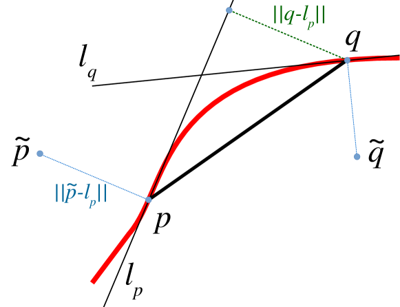
Assume there is a smooth curve, see Fig. 1. Points $p$ and $q$ on the curve and tangents $l_{p}$ and $l_{q}$ at these points are given. Then the integrals of curvature $\kappa(\cdot)$ is estimated by

$$\int_{p}^{q}|\kappa(s)|ds\;\;\approx\;\;\frac{\|p-l_{q}\|}{\|p-q\|},$$ (1)

$$\int_{p}^{q}|\kappa(s)|^{2}ds\;\;\approx\;\;\frac{\|p-l_{q}\|^{2}}{\|p-q\|^{3}}.$$ (2)

where $\|p-l_{q}\|$ is the distance between point $p$ and the tangent line at point $q$ represented by collinear vector $l_{q}$. [21] explores properties of these approximations and argues

$$\kappa_{pq}(l_{p},l_{q}):=\frac{1}{2}\frac{\|p-l_{q}\|^{2}+\|q-l_{q}\|^{2}}{\|p-q\|^{2}}$$ (3)

is a better regularizer, where we used a symmetric version of integral in (2).

Marin et al. [17] generalized this surface fitting problems to detection problems where majority of the data points, e.g. image pixels, do not belong to a thin structure. In order to do that they introduced binary variables in their energy indicating if a data point belongs to the thin structure. One of their applications is vessel detection. The proposed vessel-tree extraction system includes vessel enhancment filtering, non-maximum suppresion for data reduction, tangent approximation of vessels’ centerline and minimum spanning tree for topology extraction. Assuming that detection variables are computed, the tangent approximation of vessels’ centerline is found by minimizing energy

$$E_{u}(l)=\sum_{p}{\|\tilde{p}-l_{p}\|^{2}}+\gamma\sum_{(p,q)\in N}\kappa_{pq}(l_{p},l_{q})$$ (4)

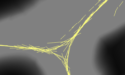
where summations are over detected vessel points, $\tilde{p}$ is the original data point’s location, $l_{p}$ is the tangent vector at point $p$, the denoised point location $p$ is constraint to be the closest point on tangent line at $p$, and $N\subset\Omega^{2}$ is the neighbourhood system. The curvature term in the energy makes the tangents “collapse” onto one-dimensional centerline as in Fig. 3(a,c). But the same figures also show artifacts around bifurcations where undesired triangular structures forms indicating unoriented tangent model limitations.

Our experiments employs the same components as in [17]. Our work focuses on analysis of failure cases and improvement of the regularization stage for tangent approximation. In particular we will show the drawbacks of curvature models (1-3) in the context of vessel tree extraction and propose a solution leading to significant improvement of the results.

1.4 Our contributions and motivation

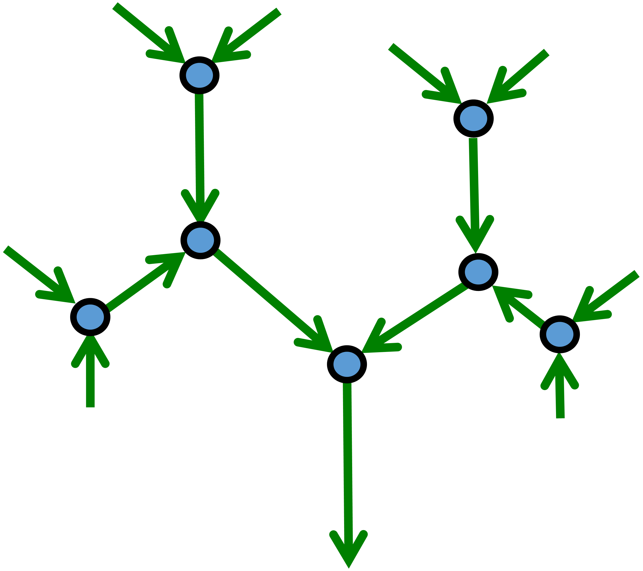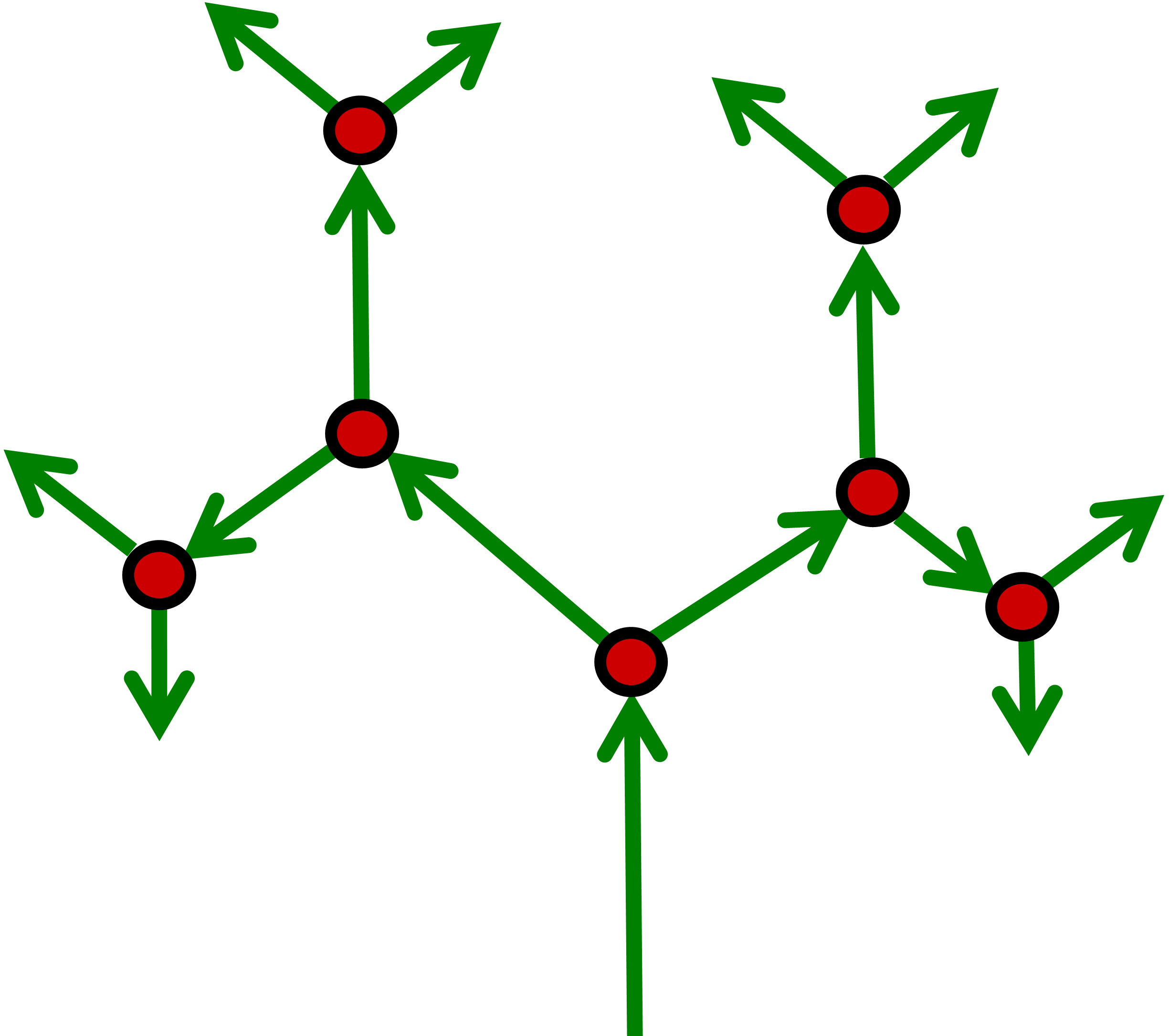
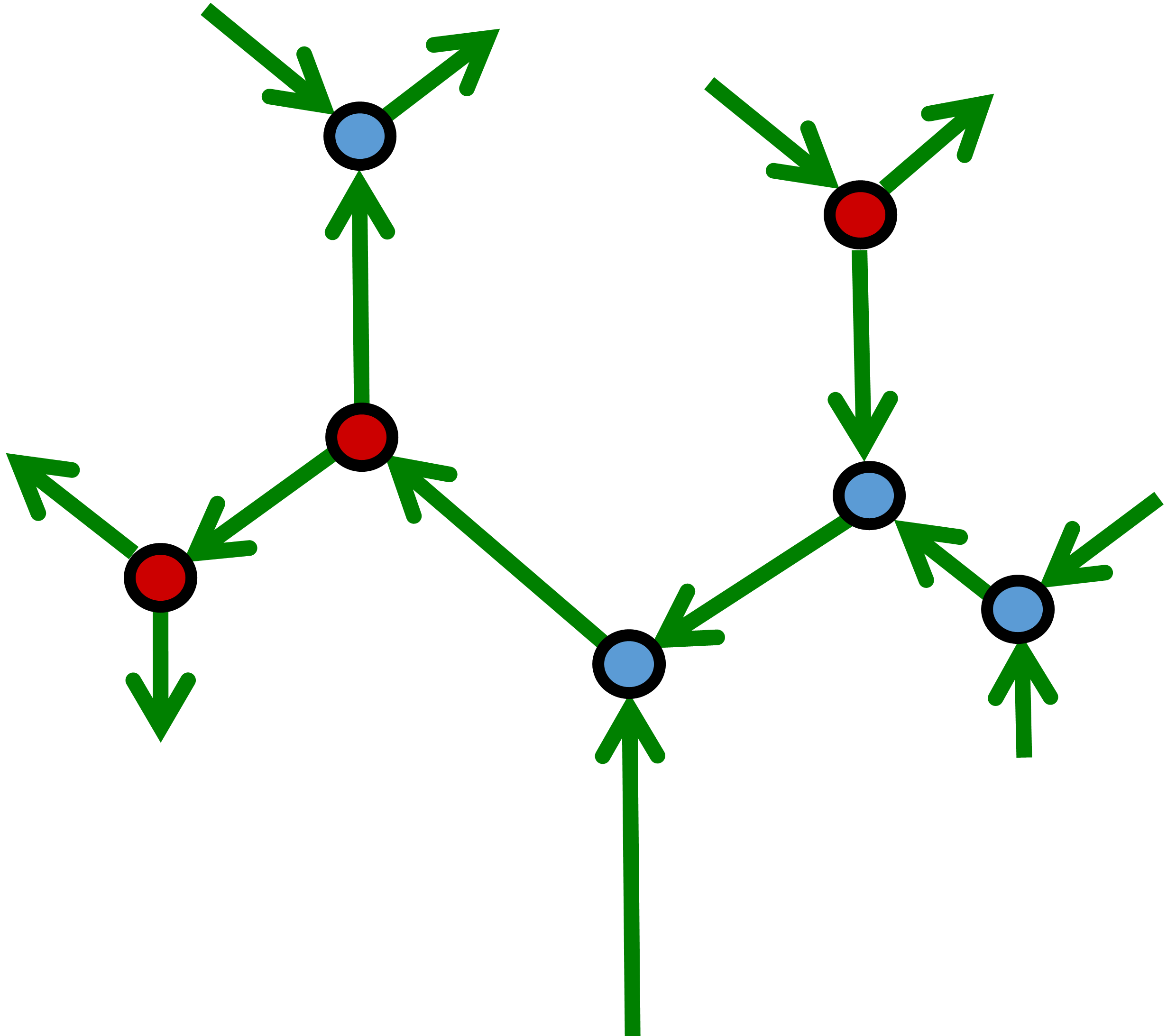
(a) divergent vessels (arteries)	(b) inconsistent divergence	(c) convergent vessels (veins)

Figure 2: [Vessel-tree divergence] Vessels are the blood flow pathlines and could be assigned orientations (7). To estimate orientations, we penalilze negative (or positive) “vessel divergence”, which we define as the divergence of oriented unit tangents of vessels/pathlines. Such unit tangent flow divergence is positive (red) or negative (blue) at bifurcations, see (a-c). Note that standard curvature [21, 17] and oriented curvature models (6) either can not distinguish (b) from (a) and (c) or may even prefer (b) depending on specific combinations of bifurcation angles. For example, compare vessel direction disambiguation based on curvature and divergence prior in Fig.7 (a) and (b).

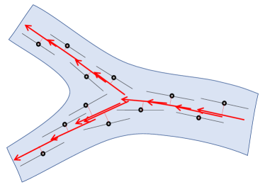
This work addresses an important limitatation of vessel tree reconstruction methods due to sign ambiguity in vessel orientation produced by local vesselness filters, e.g. Frangi. This orientation is described by the smallest eigen vector of the local intensity Hessian, but its sign is ambiguous. Thus, the actial flow directions are not known, eventhough they are an important reconstruction cue particualrly at bifurcations. This binary direction ambiguity can be resolved only by looking at the global configuration of vessel orientations (tangents) allowing to determine a consistent flow pattern.

We propose a divergence prior for disambiguating the global flow pattern over the vessel tree, see Figure 2. This prior can be imposed as a regularization constraint for a vector field of oriented unit tangents for vessel pathlines. We penalize negative (or positive) divergence for such unit tangent flow to enforce a consistent flow pattern. The summary of our contributions:

• Prior knowledge about divergence is generally useful for vector field inference. We propose a way to evaluate divergence for sparsely sampled vector fields via pairwise potentials. This makes divergence constraints amenable to a wide range of optimization methods for disrcrete of continuous hidden variables.

• As an important application, we show that known divergence can disambiguate vessel directions produced by standard vessel filters, e.g. Frangi [10]. This requires estimation of binary “sign” variables. The constraint penalizing positive (or negative) divergence is non-submodular, but it is well optimized by TRWS [14].

• To estimate vessel tree centerline, divergence constraint can be combined with robust oriented curvature regularization for pathline tangents. Additional options include outlier/detection variables [17] and/or tree structure completion techniques, e.g. using MST.

• We provide extensive quantitative validation on synthetic vessel data, as well as qualitative results on real high-resolution volumes.

The paper is organized as follows. Section 2 introduces oriented vessel pathline tangents and discusses their curvature-based regularization. It is clear that orientation of the flow at the bifurcations is important, e.g. see Fig.3. Section 3 introduces our divergence prior and methods for enforcing it in the context of vessel tree centerline estimation. The last sections presents our experimental results.

2 Bifurcations and curvature

(a)	(b)
(c)	(d)

Figure 3: Triangle artifacts at bifurcation. Optimization of energy (4) ignoring tangent orintations often leads to a strong local minima as in (a) and (c). The line segments are the estimated tangents of the centerline. New curvature term (6) takes into account tangent orientations resolving the artifacts, see (b) and (d).

2.1 Oriented curvature constraint

(a)
(b)
(c)

Figure 4: The difference between unoriented (a) and oriented (b, c) tangents. Unoriented models ignore directions of tangents (a). Red color illustrates curves that comply with tangents in unoriented (a) and oriented (b, c) cases. Curvature approximations (1–3) are not able to distinguish (a), (b) and (c). Our oriented curvature (6) prefers configuration (c) over (a) and (b).

(a)	(b)	(c)

Figure 5: Illustrative examples of three interacting tangents with unoriented curvature (a) as in energy (4) and two alternative oriented configurations (b) and (c) with oriented curvature as in energy (5). The green line denotes pairwise interaction with low curvature value. Note, that unoriented curvature (1–3) always chooses the smallest angle for calculation. The red line shows “inactive” pairwise interaction, i.e. interaction where curvature in (6) reaches the high saturation threshold.

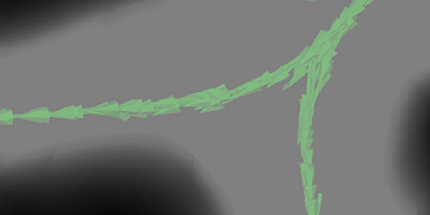
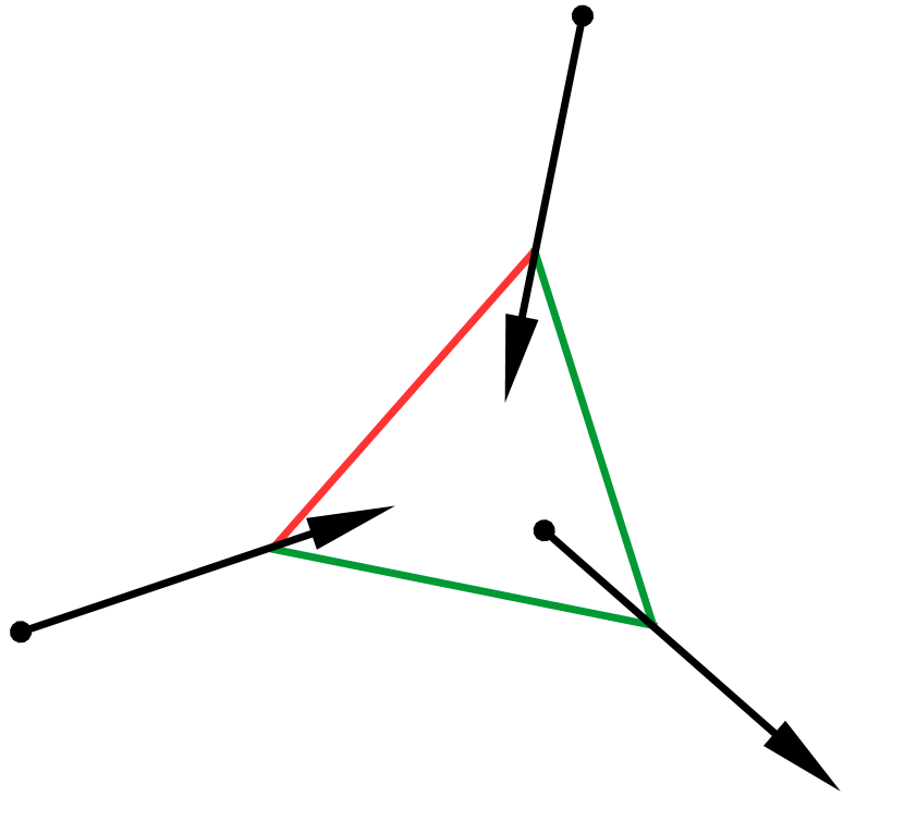
Previous works [21, 23, 17] ignored orientations of tangent vectors $\{l_{p}\}_{p\in\Omega}$. Equations (1)–(4) do not depend on orientations of $l$. In practice, the orientations of vectors $l_{p}$ are arbitrarily defined. Ingnoring the orientations in energy (4) results in significant “triangle” artifacts around bifurcation, see Fig. 3(a,c). Consider an illustrative example in Fig. 5(a). Each of three tangents interacts with the other two. The prior knowledge about blood flow pattern dictates that among those three tangents there should be one incoming and one outcoming. Introduction of orientations allows us to distinguish the incoming/outcoming tangents and subsequently inactivate one of the interactions, see Fig. 5(b), resulting in disappearance of these artifacts.

In order to introduce oriented curvature we introduce a new vector field $\bar{l}_{p}$, which we call oriented. Then, we introduce energy $E_{o}(\bar{l})$ by replacing curvature term in energy (4) with a new oriented curvature as follows

$$E_{o}(\bar{l})=\sum_{p}{\|\tilde{p}-\bar{l}_{p}\|^{2}}+\gamma\sum_{(p,q)\in N}\bar{\kappa}_{pq}(\bar{l}_{p},\bar{l}_{q})$$ (5)

where

$$\bar{\kappa}_{pq}(\bar{l}_{p},\bar{l}_{q})\;\;:=\;\;\begin{cases}\kappa_{pq}(\bar{l}_{p},\bar{l}_{q}),&\langle\bar{l}_{p},\bar{l}_{q}\rangle\geq\tau,\\ 1,&\text{otherwise,}\end{cases}$$ (6)

and $\langle\bar{l}_{p},\bar{l}_{q}\rangle$ is the dot product of $\bar{l}_{p}$ and $\bar{l}_{q}$ and $\tau\geq 0$ is a positive threshold discussed in Fig. 6.

Figure 6: Robustness of curvature (6). The pairs of tangent vectors that has angle greater than $\operatorname{acos}\tau$ are not considered belonging to the same vessel. A constant penalty is assigned to such pairs. This “turns off” smoothness enforcement at bifurcations.

The connection between oriented field $\bar{l}$ and $l$ is

$$\bar{l}_{p}=x_{p}\cdot l_{p}$$ (7)

where binary variables $x_{p}\in\{-1,1\}$ flip or preserve the arbitrarily defined orientations of $l_{p}$.

2.2 Curvature and orientation ambiguity

Introduction of orientated curvature resolves triangle artifacts, see Fig. 3(b,d). However, the orientations are not known in advance. For example, Frangi filter [10] defines a tangent as a unit eigen vector of a special matrix. The unit eigen vectors are defined up to orientation, which is chosen arbitrarily. One may propose to treat energy (5) as a function of tangent orientations $x$ via relationship (7) as follows

$$E_{o}(x)\;\;:=\;\;E_{o}(\{x_{p}\cdot l_{p}\})\Big{|}_{l_{p}=const}$$ (8)

However, energy (8) is under-constrained because it allows multiple equally good solutions, see Fig. 5(b) and (c). The example in (b) shows a divergent pattern while (c) shows a convergent pattern suggesting artery/vein ambiguity. Unfortunately, energy (8) does not enforce consistent flow pattern across the vessel tree resulting in a mix of divergent and convergent bifurcations as in Fig. 2(b). Real data experiments confirm this conclusion, see Fig. 7(a).

Thus, oriented curvature model (5) has a significant problem. While it can resolve “triangle artifacts” at bifurcations, see Fig.3, it will break the wrong sides of the triangles at many bifurcations where it estimates the flow pattern incorrectly and then give the incorrect estimation of centerline, see Fig.8(a). Below we introduce our divergence prior directly enforcing consistent flow pattern over the vessel tree.

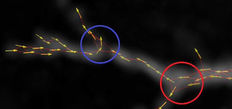(a) oriented curvature only (8)

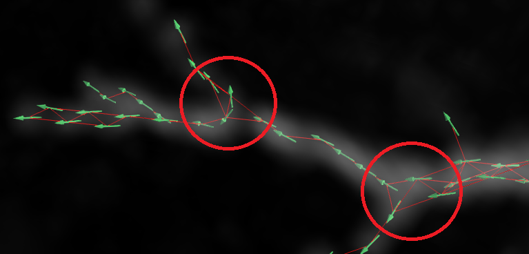(b) with divergence prior (11)

Figure 7: Disambiguating flow directions in Frangi output [10]. Both examples use fixed (unoriented) vessel tangents $\{l_{p}\}$ produced by the filter and compute (oriented) vectors $\bar{l}_{p}=x_{p}l_{p}$ (7) by optimizing binary sign variables $\{x_{p}\}$ using energies (8) in (a) and (11) in (b). The circles indicate divergent (red) or convergent (blue) bifurcations similarly to the diagrams in Fig.2. The extra divergence constraint in (10) enforces consistent flow pattern (b).

3 Divergence constraint

3.1 Estimating divergence

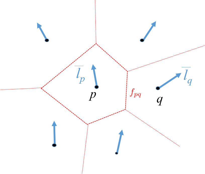
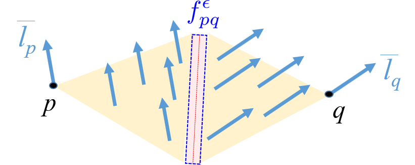
Figure 9 describes our (finite element) model for estimating divergence of a sparse vector field $\{\bar{l}_{p}|p\in\Omega\}$ defined for a finite set of points $\Omega\subset{\cal R}^{3}$. We extrapolate the vector field over the whole domain ${\cal R}^{3}$ assuming constancy of the vectors on the interior of the Voronoi cells for $p\in\Omega$, see Fig.9(a). Thus, vectors change only in the (narrow) region around the cell facets where all non-zero divergence is concentrated. To compute the integral of divergence in the area between two neighboring points $p,q\in\Omega$, see Fig.9(b), we estimate flux of the extrapolated vector field over $\epsilon$-thin box $f^{\epsilon}_{pq}$ around facet $f_{pq}$

$$\int_{f^{\epsilon}_{pq}}\langle\bar{l},n_{s}\rangle\;ds\;\;=\;\;\frac{\langle\bar{l}_{q},pq\rangle-\langle\bar{l}_{p},pq\rangle}{|pq|}\cdot|f_{pq}|\;\;+\;\;o(\epsilon)$$

where $n_{s}$ is the outward unit normal of the box and $|f_{pq}|$ is the facet’s area. Then, divergence theorem implies the following formula for the integral of divergence of the vector field inside box $f^{\epsilon}_{pq}$

$$\nabla\bar{l}_{pq}\;\;\ =\;\;\frac{\langle\bar{l}_{q},pq\rangle-\langle\bar{l}_{p},pq\rangle}{|pq|}\cdot|f_{pq}|$$ (9)

where we ignore only infinitesimally negligible $o(\epsilon)$ term.

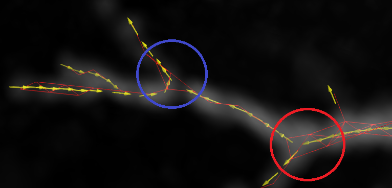(a) tangent vectors at convergence for energy (5)

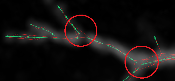(b) tangent vectors at convergence for energy (10)

Figure 8: Centerline estimation for the data in Fig.7. Instead of showing tangent orientations estimated at the first iteration as in Fig.7, we now show the final result at convergence for minimizing energy (5) in (a) and energy (10) in (b). Blue circle shows bifurcation reconstruction artifacts due to wrong estimation of vessel orientations in Fig.7(a).

(a) Voronoi cells for $p,q\in\Omega$ and facet $f_{pq}$

(b) $\epsilon$-thin box $f^{\epsilon}_{pq}$ around facet $f_{pq}$

Figure 9: Divergence of a sparse vector field $\{\bar{l}_{p}|p\in\Omega\}$. Assuming that the corresponding “extrapolated” dense vector field is constant inside Voronoi cells (a), it is easy to estimate (non-zero) divergence $\nabla\bar{l}_{pq}$ (9) concentrated in a narrow region $f^{\epsilon}_{pq}$ around each facet (b) using the divergence theorem.

3.2 Oriented centerline estimation

Constraints for divergence $\nabla\bar{l}_{pq}$ in the regions between neighbors $p,q\in{\cal D}$ in Delaugney triangulation of $\Omega$ can be combined with $E_{o}(\bar{l})$ in (5) to obtain the following joint energy for estimating oriented centerline tangents $\bar{l}_{p}$

$$E(\bar{l})\;\;=\;\;E_{o}(\bar{l})\;\;\;+\;\;\;\lambda\;\sum_{(p,q)\in{\cal D}}(\nabla\bar{l}_{pq})^{-}$$ (10)

where the negative part operator $(\cdot)^{-}$ encourages divergent flow pattern as in Fig.2(a). Alternatively, one can use $(\cdot)^{+}$ to encourage a convergent flow pattern as in Fig.2(c). This joint energy for oriented centerline estimation $E(\bar{l})$ combines Frangi measurements, centerline curvature regularity, and consistency of the flow pattern, see Fig.7(b). Note that specific value of facet size in (9) had a negligible effect in our centerline estimation tests as it only changes a relative weight of the divergence penalty at any given location. For simplicity, one may use $|f_{pq}|\approx const$ for all $p,q\in{\cal D}$.

Figure 10: Representative example of decrease in energy (10) for block-coordinate descent iterating optimization of (11) and (12). For initialization, we use raw undirected tangents $\{l_{p}\}$ generated by Frangi filter [10]. Then, we iteratively reestimate binary sign variables $\{x_{p}\}$ and unoriented tangents $\{l_{p}\}$.

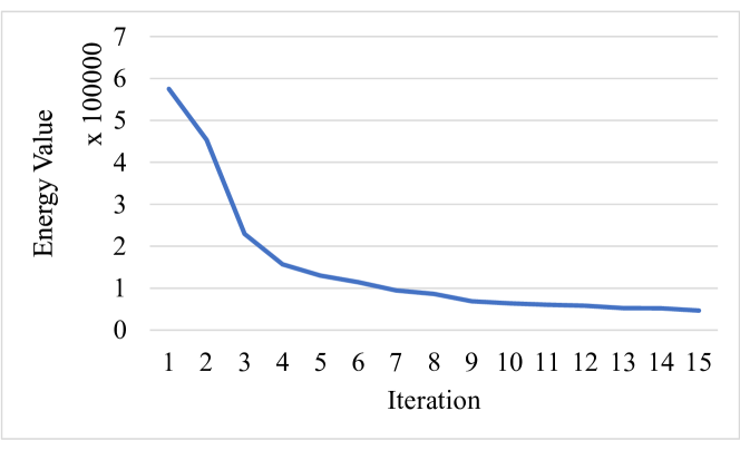
Optimization of oriented centerline energy $E(\bar{l})$ in (10) over oriented tangents $\{\bar{l}_{p}\}$ can be done via block-coordinate descent. As follows from definition (7)

$$E(\bar{l})\;\;\equiv\;\;E(\{x_{p}\cdot l_{p}\}).$$

We iterate TRWS [14] for optimizing non-submodular energy for binary “sign” disambiguation variables $\{x_{p}\}$

$$E(x)\;\;:=\;\;E(\{x_{p}\cdot l_{p}\})\Big{|}_{l_{p}=const}$$ (11)

and trust region [31, 17] for optimizing robust energy for aligning tangents into 1D centerline

$$E(l)\;\;:=\;\;E(\{x_{p}\cdot l_{p}\})\Big{|}_{x_{p}=const}.$$ (12)

Figure 10 shows a representative example illustrating convergence of energy (10) in a few iterations.

Note that the divergence constraint in joint energy (10) resolves the problem of under-constrained objective (5) discussed at the end of Section 2. Since the flow pattern consistency is enforced, optimization of (10) should lead to a consistent resolution of triangle artifacts at bifurcations. see Fig.8(b). Our experimental results support this claim.

4 Evaluation

4.1 Synthetic vessel volume

Figure 11: An example of one volume synthetic data. The white lines inside vessels denote ground truth of centerline.

Figure 12: Comparison of our method (OriAbsCurv and OriQuaCurv) with the unoriented quadratic curvature (QuaCurv) [17], non-maximum suppression (NMS), SegmentTubes (Aylward $et\ al.$ [3]) and medial axis extraction (Bouix $et\ al.$ [4]) at three different noise levels. The four letters on yellow circles denote different seed point lists. $a$: using root and all leaf points; $b$: using 50% of the mixture of all bifurcation and leaf points and root; $c$: using middle points of all branch segments; $d$: using all bifurcation and leaf points and root.

Figure 13: Comparison only at bifurcation point.

Figure 14: Angle error comparison.

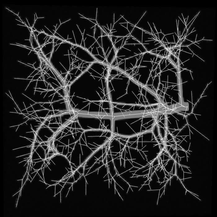
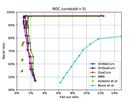
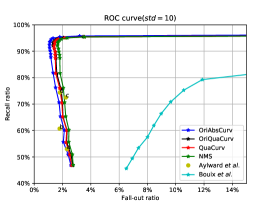
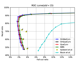
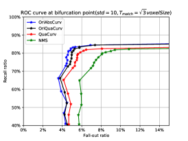
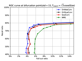
We used the modification of a method generating synthetic 3D vessel tree data [12]. The generated data consists of CT-like volume and ground truth vessel centerline tree, see Fig. 11 for an example. We generate 15 artificial volumes $100\!\times\!100\!\times\!100$ containing synthetic vascular trees with voxel intensities in the range $0$ to $512$. The size of voxel is $0.046$ mm. We use three different levels of additive Gaussian noise [15] with standard deviations 5, 10 and 15.

Evaluation setup. Our evaluation system follows [17]. We first apply Frangi filter [10] with hyperparameters $\alpha=0.5$, $\beta=0.5$, $\gamma=30$, $\sigma_{min}=0.023$ mm and $\sigma_{max}=0.1152$ mm. The filter computes tubularness

measure and estimates tangent $l_{p}$ at each voxel $p$. Then we threshold the tubularness measure to remove background pixels. Then we use non-maximum suppression (NMS) resulting in voxel set $\Omega$. We use 26-connected neighborhood system $N$. Next, we optimize our new join energy (10) to disambiguate tangent orientation and estimate centerline location, see Sec. 3.2. The hyperparameters are $\gamma=3.80$ (see energy (5)), $\lambda=18.06$ (see energy (10)), $\tau=\cos 70^{\circ}$ (see equation (6)), and the maximum number of iterations is 1500 for both TRWS and Levenberg-Marquardt. Finally, we extract oriented vessel tree centerline as the minimum spanning tree of the complete graph.

Energy (10) assumes quadratic curvature term (3). However, it is to replace it with (1) to get an absolute curvature variant of our energy.

We evaluate different regularization methods including energy (4) (QuaCurv), energy (10) with either quadratic curvature (OriQuaCurv) or absolute curvature (OriAbsCurv) within the system outline above. We also compare to a tracing method [3] and medial axis [4].

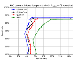
We adopt receiver operating characteristic (ROC) curve methodology for evaluation of our methods and [4]. We compute recall and fall-out statistics of an extracted vessel tree for different levels of the threshold. The computed statistics define ROC curve.

(a)	(b)	(c)	(d)

Figure 15: Examples of the result around bifurcations with regularization methods. White line is the ground truth tree. A tree extracted from NMS ouput directly (without regularization) is shown in (a). Solution of (4) [17] is (b). Our model (10) is in (c). Our model (10) with absolute curvature is in (d).

(a) cardiac microscopy CT volume

(b) zoom-in

Figure 16: Visualization (MIP) of the raw volumetric data obtained from a mouse heart by microscopic computer tomography. The data is provided by Maria Drangova from the Robarts Research Institute in London, Canada.

While ground truth is defined by locations at bifurcations and leaves of the tree, all evaluated methods yield densly sampled points on the tree. Therefore, we resample both ground truth and reconstructed tree with step size $0.0023$ mm. For each point on one tree, we find the nearest point on the other tree and compute the Euclidean distance. If the distance is less than $\max(r,c)$ voxels, this pair of points is considered a match. Here $r$ is the vessel radius at the corresponding point of the ground truth and $c=0.7$ is a matching threshold measured in voxels. The recall is

$$\frac{N_{GTmatch}}{N_{GTtotal}}$$

where $N_{GTmatch}$ is the number of matched points in the ground truth and $N_{GTtotal}$ is the total number of points in the ground truth. The fall-out is

$$1-\frac{N_{RTmatch}}{N_{RTtotal}}$$

where $N_{RTmatch}$ is the number of matched points in the ground truth and $N_{RTtotal}$ is the total number of points in the ground truth.

Figure 17: Vessel tree reconstruction from real data in Fig. 16 based on our method for estimating centerline tangents using prior knowlegde about vessel divergence. The final tree structure is extracted by MST on K-nearest-neighbour (KNN) weighted graph with edge weights $w_{pq}$ defined as the average arc-length between neighbors $p$ and $q$ for two circles containing $p$ and $q$ and tangential to either $l_{p}$ or $l_{q}$. Three different colors (red, blue, yellow) denote three main branches.

Figure 18: Qualitative comparison results on real data. Red represents the result of [17], see (4). Blue curve is the centerline obtained based on our directed vessel estimation model (10) with divergence prior and absolute curvature regularization. The yellow circles highlight improvements at bifurcations due to correct estimation of the flow direction.

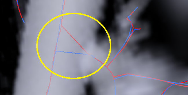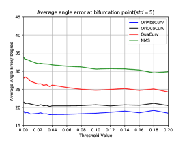
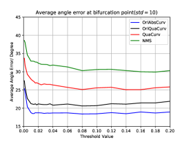
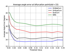
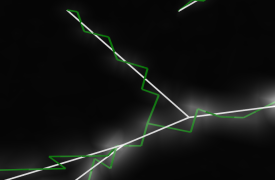
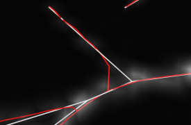
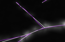
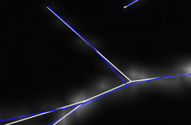
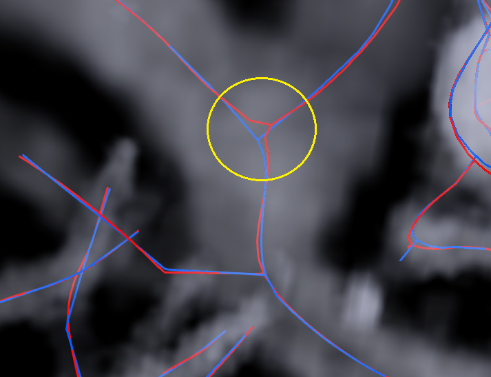
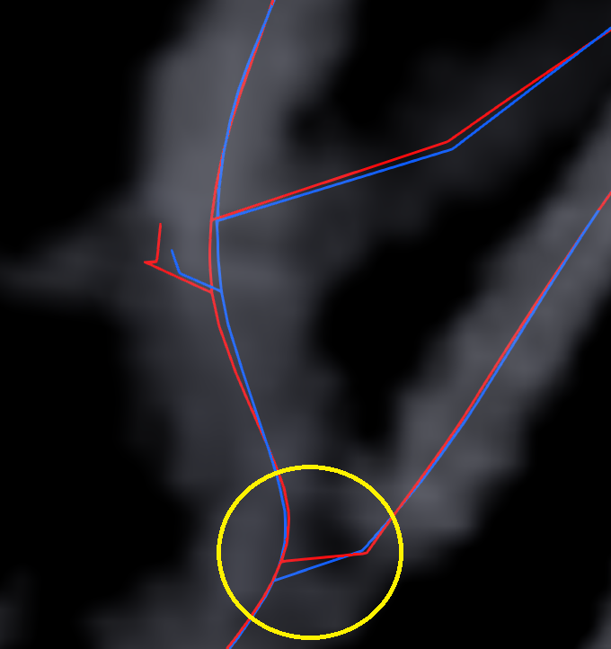
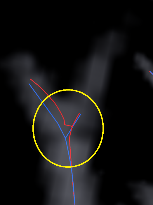
The tracing method of [3] requires a seed points list as an input. We generate four seed lists as described in Fig. 12. The ROC curves in Fig. 12 favour our method. Since bifurcations is only a fraction of the data, the improvements around bifurcations are largely unnoticed in these curves. Therefore, we compute the ROC curves for only bifurcation nodes. We use a bigger matching threshold $c=\sqrt{3}$ voxels. The results are shown in Fig. 13 where the gap between methods is bigger. Also we compute angle errors at bifurcations, see Fig. 14 and few examples in Fig. 15.

4.2 Real vessel data

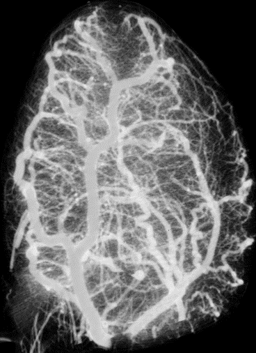
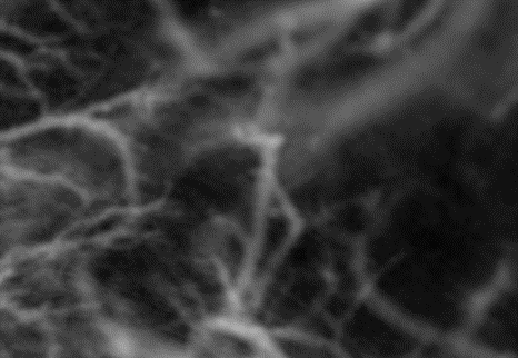
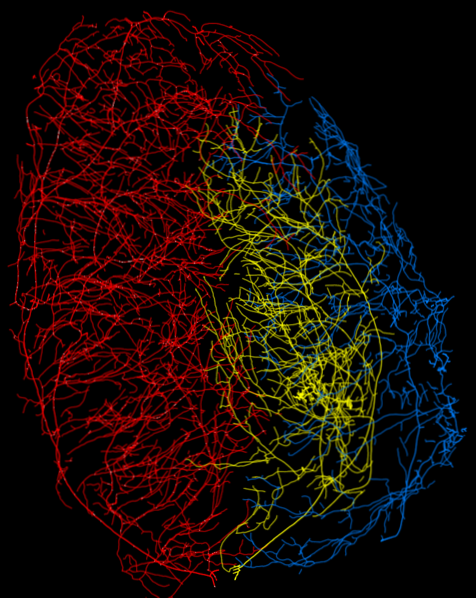
We obtained the qualitative experimental results using a real micro-CT scan of mouse’s heart as shown in Figure 16. The size of the volume is $585\times 525\times 892$ voxels. Most of the vessels are thinner than voxel size. Due to the size of the volume the problem has higher computational cost than in Sec. 4.1. We built custom GPU implementation of Levenberg-Marquardt algorithm to handle the large volume size. Figure 17 shows the reconstructed centerline. Figure 18 demostrate significant improvement of centerline estimation around bifurcations.

5 Conclusions and Future work

We propose divergence prior for vector field reconstruction problems. In the contest of vessel tree estimation, we use divergent vessel prior to estimate vessel directions disambiguating orientations produced by Frangi filter. Our method significnatly improves the accuracy of reconstruction at bifurcations reducing the corresponding angle estimation errors by about 50 percent.

There are interesting extentions for our work on estimating vessel orientations. For example, such orientations can be directly used for extracting vessel tree topology or connectivity. Instead of using standard MST on undirected graphs, e.g. as in [17], we can now use Chu-Liu-Edmonds algorithm [7, 8] to compute a minimum spanning arborescence (a.k.a. directed rooted tree) on a directed weighted graph where a weight of any edge $(p,q)$ estimates the length of a possible direct “vessel” connection specifically from $p$ to $q$. Such a weight can estimate the arc length from $p$ to $q$ along a unique circle such that it contains $p$ and $q$, it is coplanar with $l_{p}$ and $q$, and it is tangential to $l_{p}$. However, such constant curvature path from $p$ to $q$ works as a good estimate for a plausible vessel connection from $p$ to $q$ only if $\langle l_{p},pq\rangle>0$; otherwise there should be no edge from $p$ to $q$. This implies a directed graph since edges $(p,q)$ and $(q,p)$ will be determined by two different tangents $l_{p}$ or $l_{q}$ and two different conditions $\langle l_{p},pq\rangle>0$ or $\langle l_{q},qp\rangle>0$.

References

- [1] T. D. Alter and R. Basri. Extracting salient curves from images: An analysis of the saliency network. IJCV, 27(1):51–69, 1998.
- [2] L. Alvarez, P.-L. Lions, and J.-M. Morel. Image selective smoothing and edge detection by nonlinear diffusion. ii. SIAM Journal on numerical analysis, 29(3):845–866, 1992.
- [3] S. R. Aylward and E. Bullitt. Initialization, noise, singularities, and scale in height ridge traversal for tubular object centerline extraction. IEEE transactions on medical imaging, 21(2):61–75, 2002.
- [4] S. Bouix, K. Siddiqi, and A. Tannenbaum. Flux driven automatic centerline extraction. Medical image analysis, 9(3):209–221, 2005.
- [5] K. Bredies, T. Pock, and B. Wirth. Convex relaxation of a class of vertex penalizing functionals. Journal of Mathematical Imaging and Vision, 47(3):278–302, 2013.
- [6] T. F. Chan and J. Shen. Nontexture inpainting by curvature-driven diffusions. Journal of Visual Communication and Image Representation, 12(4):436–449, 2001.
- [7] Y. J. Chu and T. H. Liu. On the shortest arborescence of a directed graph. Science Sinica, 14:1396–1400, 1965.
- [8] J. Edmonds. Optimum branchings. J. Res. Nat. Bur. Standards, 71B(4), October- December 1967.
- [9] A. Enquobahrie, L. Ibanez, E. Bullitt, and S. Aylward. Vessel enhancing diffusion filter. The Insight Journal, 1:1–14, 2007.
- [10] A. F. Frangi, W. J. Niessen, K. L. Vincken, and M. A. Viergever. Multiscale vessel enhancement filtering. In MICCAI’98, pages 130–137. Springer, 1998.
- [11] G. Guy and G. Medioni. Inferring global perceptual contours from local features. In CVPR, 1993.
- [12] G. Hamarneh and P. Jassi. Vascusynth: simulating vascular trees for generating volumetric image data with ground-truth segmentation and tree analysis. Computerized medical imaging and graphics, 34(8):605–616, 2010.
- [13] S. Heber, R. Ranftl, and T. Pock. Approximate envelope minimization for curvature regularity. In ECCV, 2012.
- [14] V. Kolmogorov. Convergent tree-reweighted message passing for energy minimization. PAMI, 28(10):1568–1583, 2006.
- [15] G. Lehmann. Noise simulation. The Insight Journal, January-June 2010.
- [16] G. Li and S. W. Zucker. Differential geometric inference in surface stereo. PAMI, 32(1):72–86, 2010.
- [17] D. Marin, Y. Zhong, M. Drangova, and Y. Boykov. Thin structure estimation with curvature regularization. In International Conference on Computer Vision (ICCV), Santiago, Chile, December 2015.
- [18] S. Moccia, E. De Momi, S. El Hadji, and L. Mattos. Blood vessel segmentation algorithms — review of methods, datasets and evaluation metrics. Computer Methods and Programs in Biomedicine, 158:71–91, 2018.
- [19] P. MomayyezSiahkal and K. Siddiqi. 3d stochastic completion fields for mapping connectivity in diffusion mri. PAMI, 35(4):983–995, 2013.
- [20] C. Nieuwenhuis, E. Toeppe, L. Gorelick, O. Veksler, and Y. Boykov. Efficient squared curvature. In CVPR, Columbus, Ohio, 2014.
- [21] C. Olsson and Y. Boykov. Curvature-based regularization for surface approximation. In Conference on Computer Vision and Pattern Recognition (CVPR), pages 1576–1583. IEEE, 2012.
- [22] C. Olsson, J. Ulén, and Y. Boykov. In defense of 3d-label stereo. In CVPR, pages 1730–1737. IEEE, 2013.
- [23] C. Olsson, J. Ulén, Y. Boykov, and V. Kolmogorov. Partial enumeration and curvature regularization. In ICCV, pages 2936–2943. IEEE, 2013.
- [24] T. Schoenemann, F. Kahl, and D. Cremers. Curvature regularity for region-based image segmentation and inpainting: A linear programming relaxation. In ICCV, Kyoto, 2009.
- [25] T. Schoenemann, F. Kahl, S. Masnou, and D. Cremers. A linear framework for region-based image segmentation and inpainting involving curvature penalization. IJCV, 2012.
- [26] K. Siddiqi and S. Pizer. Medial representations: mathematics, algorithms and applications, volume 37. Springer Science & Business Media, 2008.
- [27] P. Strandmark and F. Kahl. Curvature regularization for curves and surfaces in a global optimization framework. In EMMCVPR, pages 205–218. Springer, 2011.
- [28] M. Tang, F. Perazzi, A. Djelouah, I. B. Ayed, C. Schroers, and Y. Boykov. On regularized losses for weakly-supervised cnn segmentation. In European Conference on Computer Vision (ECCV), Munich, Germany, September 2018.
- [29] L. R. Williams and D. W. Jacobs. Stochastic completion fields: A neural model of illusory contour shape and salience. Neural Computation, 9(4):837–858, 1997.
- [30] O. Woodford, P. Torr, I. Reid, and A. Fitzgibbon. Global stereo reconstruction under second-order smoothness priors. PAMI, 31(12):2115–2128, 2009.
- [31] S. Wright and J. N. Holt. An inexact levenberg-marquardt method for large sparse nonlinear least squres. The Journal of the Australian Mathematical Society. Series B. Applied Mathematics, 26(04):387–403, 1985.