Towards Emotion Recognition: A Persistent Entropy Application

Abstract

Emotion recognition and classification is a very active area of research. In this paper, we present a first approach to emotion classification using persistent entropy and support vector machines. A topology-based model is applied to obtain a single real number from each raw signal. These data are used as input of a support vector machine to classify signals into $8$ different emotions (calm, happy, sad, angry, fearful, disgust and surprised).

Keywords Persistent Homology  $\cdot$ Persistent Entropy  $\cdot$ Emotion Recognition  $\cdot$ Support Vector Machine.

1 Introduction

Emotion recognition is not a trivial task and different approaches have been explored so far (see for example [1]). Additionally, its applications are really important, such as gathering and processing satisfaction feedback in customers’ services, generating statistical studies over a population, using emotion recognition to improve spoken language understanding during a conversation. Furthermore, it can help in human interaction as in KRISTINA project, where emotion recognition is applied in order to help the interaction between health professionals and migrated patients. Among the different theories about emotions proposed in the specialized literature, we follow the model described in [2] and [3], where a discrete theory of emotions is given, differentiating several basic groups of emotions (neutral, happy, sad and surprised) and organizing them in a spatial model. In [4] a review of different emotional speech recognition techniques can be consulted.

Topological data analysis is a well substantiated field useful to extract information from data (see [5]). Concretely, a recent tool in this area called persistent entropy has been successfully applied to distinguish discrete piecewise-linear functions (see [6]).

In this paper, persistent entropy is used to model arousal (i.e., emotional state) and emotion recognition as follows. First, speech signals are considered as piecewise linear functions. Second, persistent entropy is computed from the lower-star filtration obtained from these functions. This persistent entropy embedding can be considered as a summary of the features that appear in raw signals, as intensity and intonation. The stability theorem for persistent entropy computed from lower-star filtrations [6] guarantees right comparison between signals and robustness against noise. Finally, a support vector machine is used to classify emotions via persistent entropy values. As far as our knowledge, no topology approaches have been previously applied to emotion recognition.

This paper is organized as follows: Basic emotion theory, the notions of persistent homology and persistent entropy, and machine learning knowledge required for the model are introduced in Section 2. In Section 3, the methodology followed in the experiments is explained. Results obtained from different training approaches are shown in Section 4. Finally, Section 5 provides conclusions and future work ideas.

2 Background

In this paper, different tools are mixed up in order to propose a unified and coherent framework for emotion classification. In this section, the basic concepts about acoustics, topology, machine learning and statistics are introduced.

Acoustic and Psychoacoustic Features. Emotions constitute the main field largely studied by psychologists. Following [3], we consider that emotions can be modeled spatially in a circle, being arousal and valence their main characteristic features. Accordingly, prosodic attributes of speech [7] are strongly related with emotion recognition. This research area takes into account several features of speech, in conjunction with gesticulation of the speaker. Some of those features are: pitch signal, number of harmonics, vocal tract, and speech energy.

Along this paper, just the physical features of the acoustic signal along with the processing results available from this signals (such as the contour of speech signal which is a feature affected by the arousal of the speaker), will be taken into account. The inclusion of visual features will be proposed in Section 5 as a natural continuation of this research. Sentences will be processed, assuming that certain attributes, like the fundamental frequency, intensity and duration, of a sound are meaningful for emotion production and recognition. These attributes are encapsulated under the notion of prosody. Depending on the prosodic pattern, a sentence can have very different emotional features. For example, happiness is linked usually with large fundamental frequency and, loudness, in contrast with sadness, normally related to the opposite. For further explanations about psychoacoustics, [8] can be consulted.

In the literature, some emotion classification techniques have been proposed (see [9]). Some of them employ prosody contours information of speech in order to recognize emotions, as, for example: artificial neural networks, the multichannel hidden Markov model, and the mixture of hidden Markov models. For a further approximation to paralinguistic theory see [10].

Topology background. Topological data analysis (TDA) studies the shape of data. In our case, we apply topological data analysis tools to distinguish between piecewise linear function shapes. For an introduction to topological data analysis, [11] can be consulted.

Persistent entropy is the main tool from TDA that will be used in this paper. It sums up persistent homology information which “measures" homological features of shapes and of functions.

Informally, homology provides the number of $n$-dimensional holes, called the $n$-th Betti numbers and denoted by $\beta_{n}$. Intuitively, $\beta_{0}$ is the number of connected components, $\beta_{1}$ the number of tunnels and $\beta_{2}$ the number of cavities. However, for dimensions higher than $2$, we lose the intuition about what a hole is.

Definition 1 (Betti number, informal, [12])

If $X$ is a topological space, then $H_{n}(X)\simeq\mathbb{Z}^{\beta_{n}}$ is called the $n$-th homology group of $X$ if the power $\beta_{n}$ is the number of independent $n$-dimensional ’holes’ in $X$. We call $\beta_{n}$ the $n$-th Betti number of $X$. Finally, the homology of $X$ is defined as $H(X)=\{H_{n}(X)\}^{\infty}_{n=0}$.

Observe that the concept of homology is not useful in practice. For example, suppose a dataset $V$ of $10$ points sampling a circumference. We expect that $H_{0}(V)\simeq\mathbb{Z}$ since a circumference has one connected component. However, the exact $0$-th homology of $V$ is $\mathbb{Z}^{10}$. Therefore, we need a tool to compute the homology of the underlying space sampled by a dataset. Following this idea, Edelsbrunner et al. [11] introduced the concept of persistent homology together with an efficient algorithm and its visualization as a persistence diagram. Carlsson et al. [13] reformulated and extended the initial definition and gave an equivalent visualization method called persistence barcodes.

Given a dataset $V$ and a simplicial complex $K$ constructed from it, persistent homology measures homology by a filtration during time, obtaining births and deaths of each homology class (’hole’). Consequently, those classes that persist are better candidates to be representatives of the homology of the underlying space.

Definition 2 (Abstract simplicial complex)

Let $V$ be a finite set. A family $K$ of subsets of $V$ is an abstract simplicial complex if for every subsets $\sigma\in K$ and $\mu\subset V$, we have that $\mu\subset\sigma$ implies $\mu\in K$. A subset in $K$ of $m+1$ elements of $V$ is called a $m$-simplex and $V$ is called the set of vertices of $K$.

Definition 3 (Filtration)

Given a set $V$ and a simplicial complex $K$ constructed from it, a filtration is a finite increasing sequence of simplicial complexes:

$$\emptyset=K_{0}\subset K_{1}\subset K_{2}\subset\dots\subset K_{n}=K$$

A particular filtration that will be used in this paper is the lower-star filtration.

Definition 4 (Lower-star filtration [11])

Let $K$ be a simplicial complex with real (distinct) values specified on the set $V$ of all the vertices in $K$. Since vertices have distinct function values, then they can be ordered incrementally:

$$f(u_{1})<f(u_{2})<\dots<f(u_{n}).$$

The lower star of $u_{i}$ is the subset of simplices of $K$ for which $u_{i}$ is the vertex with maximum function value,

$$K_{i}=\{\sigma\in K\ :\ \mbox{for all vertex}\ v\mbox{ of }\sigma\Rightarrow f(v)\leq f(u_{i})\}.$$

Table 1: Left: Lower-star filtration. Right: The associated persistence barcode of the corresponding lower-star filtration pictured on the left.

Once the lower-star filtration is obtained, persistent homology can be computed as follows. The inclusion $K_{i}\subset K_{j}$ induces a homomorphism $f^{i,j}:H(K_{i})\rightarrow H(K_{j})$ on homology. Its image is the persistent homology, letting $\beta_{p}^{ij}$ be the number of $n$-dimensional ‘holes’ that are born at $K_{i}$ and die entering $K_{j}$. During the computation of persistent homology along the filtration, an elder rule is applied. For example, when there are two connected components that get joined at some $K_{j}$, the older one (the one that was born earlier) remains, and the younger one dies. A persistence barcode is a representation of births and deaths of homology classes along time using bars. An example is shown in Fig. 1.

Finally, once persistence barcodes are obtained, persistent entropy can be computed.

Definition 5 (Persistent entropy [6])

Given a filtered simplicial complex $\{K(t)\ :\ t\in F\}$, and the corresponding persistence barcode $B=\{a_{i}=[x_{i},y_{i})\ :\ i\in I\}$, the persistent entropy $E$ of the filtered simplicial complex is calculated as follows:

$$E=-\sum_{i\in I}p_{i}log(p_{i})$$

where $p_{i}=\frac{l_{i}}{L},l_{i}=y_{i}-x_{i}$, and $L=\sum_{i\in I}l_{i}$. In the case of an interval with no death time, $[x_{i},\infty)$, the corresponding barcode $[x_{i},m)$ will be considered, where $m=\max{\{F\}}+1$.

The robustness of persistent homology to noise is guaranteed thanks to the following result, letting a stable comparison between signals.

Theorem 1 ([6])

Given two functions, $f:V\rightarrow R$ and $g:V\rightarrow R$, defined on a set of vertices $V$ of $\mathbb{R}^{n}$, then for every $\varepsilon>0$, there exists $\delta>0$ such that

$$||f-g||_{\infty}\leq\delta\Rightarrow|E(f)-E(g)|\leq\varepsilon.$$

Machine Learning Background. Machine learning techniques are nowadays widely applied to solve classification problems.

A classification technique will use a ‘training’ dataset

$$D=\{\ (\vec{v}_{i},c_{i})\ |\ \vec{v}_{i}\in\mathbb{R}^{n},\ c_{i}\in\{0,\dots,k\},\ i\in\{1,\dots,m\}\ \}$$

where $\{0,\dots,k\}$ are the different possible classes. From this dataset, the classification algorithm will produce a classification model. This model can lately be applied to new inputs in order to predict the corresponding classes. There exist several classification techniques in machine learning. In our case, we focus our attention on support vector machine (see [14], [15], [16] and [17, Chapter 5].

A support vector machine is a supervised learning technique that construct a hyperplane, driven by a linear function $b+\sum_{i=1}^{m}\alpha_{i}\vec{v}_{i}^{T}\vec{v}_{i}$, or a set of them that can be used to classify data. When this data is not linearly separable, a kernel trick is applied: the space is mapped to higher dimensions using a kernel function, $k(\vec{v},\vec{v}^{\prime})=\phi(\vec{v})^{T}\cdot\phi(\vec{v}^{\prime})$. Therefore, a support vector machine just creates hyperplanes that work as decision boundaries for classification after applying a deformation of the dataset in order to get a linearly separable representation. Then, formally, a support vector machine within a kernel makes predictions using the following function:

$$f(\vec{v})=b+\sum_{i=1}^{m}\alpha_{i}k(\vec{v},\vec{v}_{i})$$

where $\alpha$ is a vector of coefficients, $k$ the kernel and $b$ is a bias term. Finally, the coefficients are chosen as a result of an optimization problem of the separation margin between classes. Different kernel-based functions can be used, for example:

Kernels
Linear	$k(\vec{v},\vec{v}^{\prime})=\vec{v}^{T}\cdot\vec{v}^{\prime}$
Polynomial of degree $d$	$k(\vec{v},\vec{v}^{\prime})=(\vec{v}^{T}\cdot\vec{v}^{\prime}+c)^{d}$
Gaussian	$k(\vec{u},\vec{v})=\mathcal{N}(\vec{u}-\vec{v};0,\sigma^{2}\vec{I})$

where $\mathcal{N}(\vec{v};\vec{\mu},\Sigma)$ is the standard normal density.

Performance Metrics. Basically, we are dealing with a classification problem. Therefore, our main metric will be the accuracy, considered as the percentage of well classified data in a dataset:

$$\mbox{Accuracy}=\frac{m}{n}$$

where $m$ is the number of well-classified data and $n$ is the size of the full dataset used in the test.

Statistical Tool. The correlation coefficient of two random variables is a measure of their linear dependence. One correlation coefficient largely known and applied is the Pearson’s correlation coefficient [18]:

$$\mbox{Pearson's correlation coefficient }\rho(A,B)=\frac{cov(A,B)}{\sigma_{A}\sigma_{B}}$$

where $cov(A,B)$ is the covariance and $\sigma$ the standard deviation.

3 Methodology

As was previously anticipated, the shape of the wave of a speech signal can be meaningful to emotional speech recognition. Roughly speaking, we will compute persistent entropy to the lower-star filtration of the raw signal and then, we classify the signals by comparing these numbers using a support vector machine.

Let us now explain in details the methodology applied in this paper:

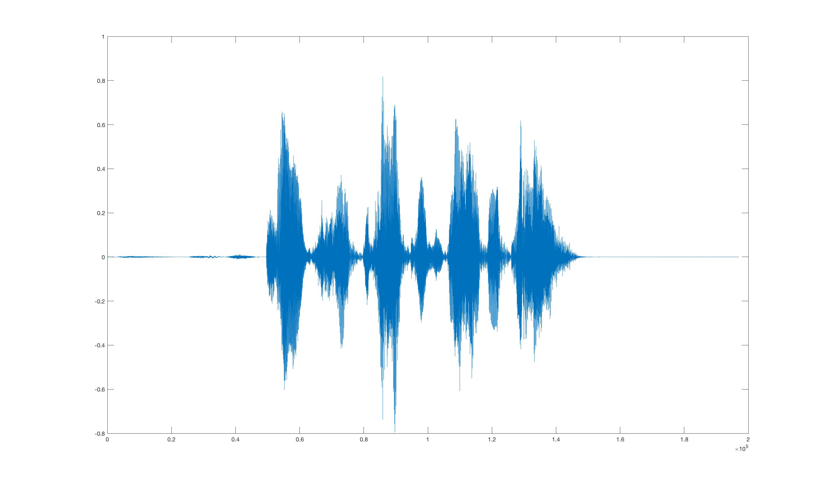
Step 1. Subsampling of the signal. The size of each signal is reduced in order to face the complexity of the persistent homology algorithm. Besides, every signal of the dataset needs to be subsampled into the same size in order to fulfill the assumptions of Theorem 1. For example, we subsampled the signal pictured in Fig. 1 from 196997 points to 10000. The subsampling process was done uniformly on the signal, maintaining its shape and main distribution of the spikes. Furthermore, the experiments of Section 4 were also done using the dataset without subsampling reaching similar results. Then, we could assert that this type of subsampling does not loose relevant information for this approach.

Figure 1: Raw signal intensity graph of an angry emotion interpreted by the actor number 1 of the RAVDESS dataset.

Step 2. Introduction of imperceptible noise. Signals are slightly perturbed to fulfill the requirement of lower-start filtrations (see Definition 4): two points in the signal can not have the same height.

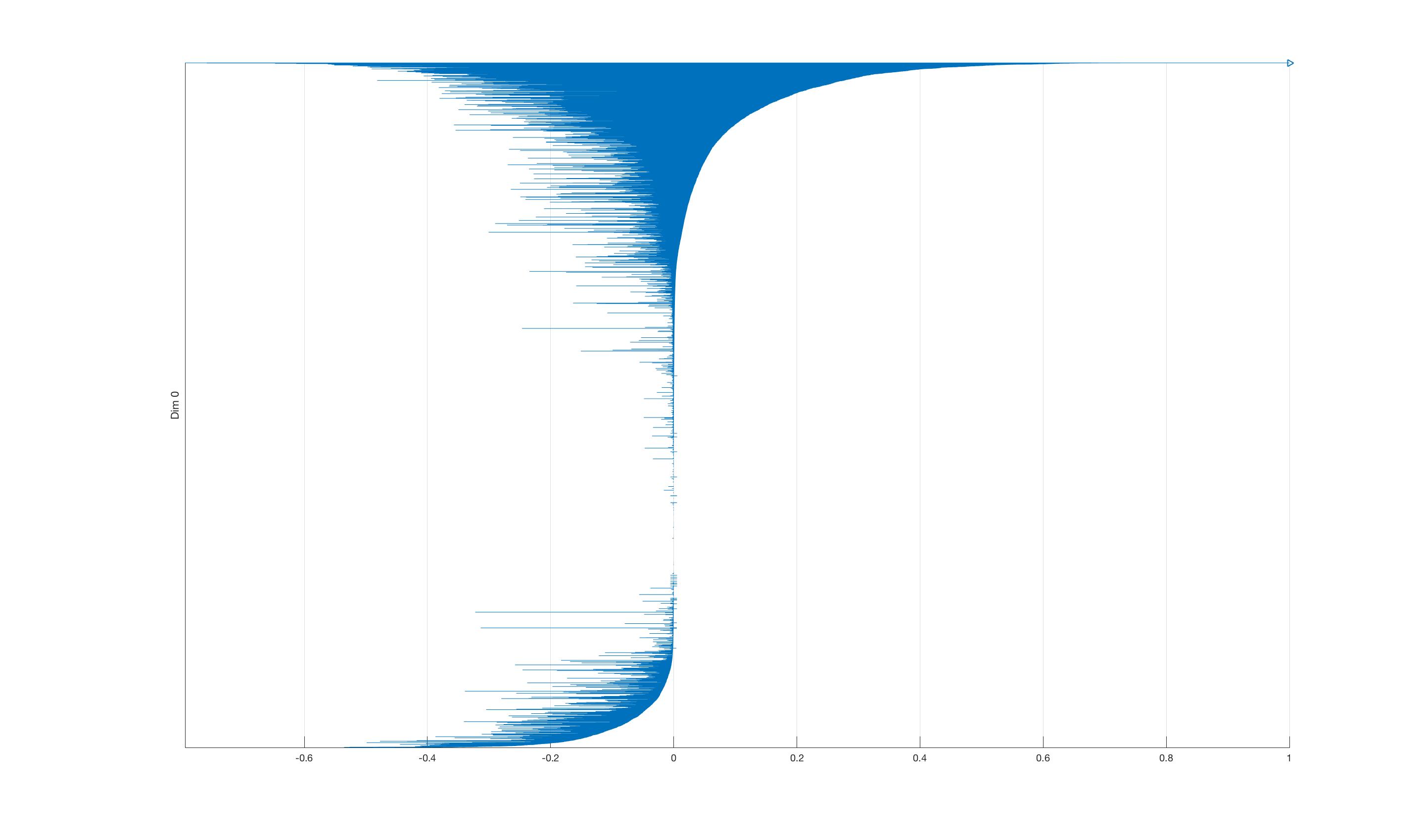
Step 3. Persistence barcode computation. The lower-star filtration technique is applied to the signals generated in Step 2, obtaining the associated persistence barcode. For example, the barcode associated to the signal of Fig. 1 can be seen in Fig. 2.

Figure 2: Barcode of the signal shown in Fig. 1. The horizontal axis represents time. Every horizontal (blue) line represents the life of a 0-dimensional homology class.

Step 4. Persistent entropy computation. Persistent entropy is computed applying the formula given in Definition 5 to the persistence barcodes obtained in Step 3.

Step 5. Support vector machine classification. This step consists of the application of several support vector machines with different kernels in order to infer results and develop a classification predictor to emotions. The different possible kernels, previously introduced in the paper, are tested and the one with better accuracy is chosen.

4 Experiments

The work-flow presented in the previous section was applied to the RAVDESS dataset [19]. This dataset is composed by $24$ actors interpreting $60$ audios each on different emotions and different intensity. Concretely, there are $4$ audios for the neutral emotion and $8$ audios for each of the seven remaining emotions. Consequently, there are $1440$ different audios.

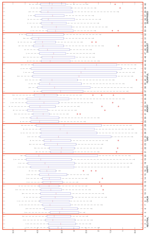
In Fig. 3, a box-plot of the persistent entropy of the $1440$ audios grouped by the different emotions can be seen. We can infer that persistent entropy values vary depending on both the emotion and the person. It seems that there exists characteristic personal values and the range of every emotion can be really wide. For example, the persistent entropy values of the audio number $20$ in Fig. 3, that is an example of happiness, varies from $5.1713$ to $0.6923$ depending on the person. Besides, the existing overlapping between the boxes tells us that emotions can not be distinguished from the rest by just the persistent entropy values of every script as a feature. This failure approximation is illustrated and explained in Experiment 1. However, some emotions can be differentiated by pairs even with this ‘naive’ approximation.

Figure 3: (90° rotated figure) Horizontal axis represents the different $60$ audios. Vertical axis represents persistent entropy. The big (red) rectangle clusters encloses persistent entropies of the audios per emotion (the respective emotion is indicated in the horizontal axis. The small (blue) rectangles are quartiles for the persistent entropy values. The vertical (blue) dashed lines mean the range of values of persistent entropy values. The (red) points are outliers. The horizontal (red) small lines are the mean persistent entropy value for the corresponding audio.

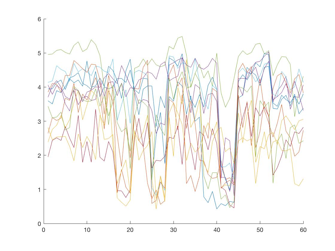
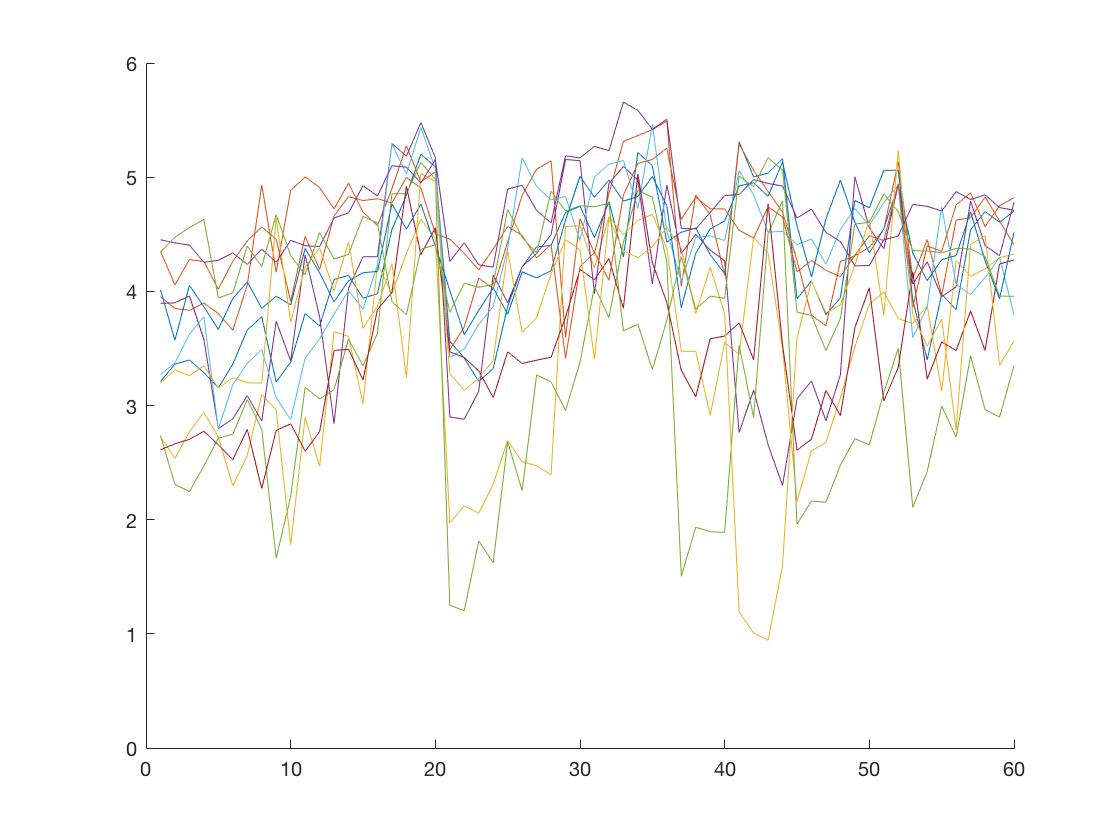
One thing that appealed our attention is the visual correlation that persistent entropy values tend to have per sexes as shown in Fig. 4 and Fig. 5. Even if the range is lower or higher depending on the person, in general, the peaks appear on the same places. To illustrate it, let us consider the correlation matrix between persistent homology values of the $60$ audios grouped in the ones belonging to females and the ones belonging to males. We obtain that persistent entropy values are moderately correlated between same sex audios and badly correlated between different sexes (see Table 2). We think that it could be interesting the use of more sophisticated measures of similarity apart from correlation. Furthermore, correlation results give us clues to the need of developing emotion classification within the dataset separated by sexes to reach better classification accuracy. Besides, we consider that persistent entropy values could even be a nice approach to people identification and not just to emotion recognition. However, this approach is far from the scope of this paper and its preliminary nature.

Figure 4: Horizontal axis represents the different audios of actresses. Vertical axis represents persistent entropy value. The different persistent entropy values for the 60 audios of the same actress are connected by an straight line. We can see that shapes are correlated (see Table 2), showing that they tend to have the same peaks and downs.

Figure 5: Horizontal axis represents the different audios of male actors. Vertical axis represents persistent entropy value. The different persistent entropy values for the 60 audios of the same actor are connected by an straight line. We can see that shapes are correlated (see Table 2), showing that they tend to have the same peaks and downs.

	Male actor	Female actor
Male actor	0.43	0.23
Female actor	0.23	0.49

Table 2: Mean values for the correlation coefficients of the entropy values grouped by sexes.

In all the following experiments we use as the classification technique a support vector machine with fold cross validation and the kernel that provides the better accuracy from the ones explained previously. The training dataset will be the $1440$ persistent entropy values grouped by different ways trying to get the features needed to reach our goal. In the first experiment we try the brute force approach using every script as a point of the training dataset. Then, in the second experiment, every point correspond to an emotion within its $24$ persistent entropy values by the $24$ different actors. Finally, in the last experiment, the dataset is grouped by actors and emotions.

Experiment 1: Each persistent entropy value will be a point of the training dataset. In this case, $20.3\%$ of accuracy is reached within a linear kernel. Some conclusions can be pointed out from this failed approach: The emotion recognition problem is a multidimensional one, in the sense that a 1-dimensional embedding is not enough to an acceptable classification result. Furthermore, this was anticipated by the overlapping of the different boxes at the box-plot of persistent entropy values showed in Fig. 3. Besides, the non correlation between persistent entropy values per sexes is a matter not taken into account in this experiment.

Experiment 2: Each point of the dataset is a vector of $24$ features which correspond to the persistent entropy value of the same emotion interpreted by the $24$ different actors. The dataset was separated in $40$ points for training dataset and $20$ points for test dataset and a gaussian kernel was used. Then, $92.5\%$ of accuracy was reached on the training dataset and $90\%$ on the test dataset. Furthermore, $96.66\%$ accuracy was obtained on the full dataset. In our opinion, this experiment presents two main drawbacks. The first one is its difficult applicability as it needs $24$ features of every emotion. However, withing long audio recordings, it could be cut into pieces and obtain enough features to classify. The other drawback is the small dataset we have for this experiment because of the way it has been grouped.

Experiment 3: In this experiment, each point of the dataset consists of a vector of $8$ features, corresponding each feature to the persistent entropy value of the same emotion interpreted by the same actor. By this, the following accuracy Table 3 for classification by pair of emotions was obtained using a second degree polynomial kernel. Considering other results in the literature like [1] where $71\%$ of accuracy was reached using Artificial Neural Networks, our results are really promising. However, we are still far from the $83\%$ of accuracy reached in [20] using a multi-task hierarchical model. But we can say that, with just a first approximation, we could reach similar accuracy than those that already exist in the literature. Furthermore, as we are considering here just intensity and one type of filtration, only some features that characterize emotions are taken into account. Then, it gives us a nice starting point in order to improve the model by using different features of the signal and different filtrations.

Feelings	Calm	Happy	Sad	Angry	Fearful	Disgust	Surprised
Calm		77.1%	68.8%	81.2%	79.2%	72.9%	60.4%
Happy			62.5%	64.6%	60.4%	58.3%	64.6%
Sad				75%	62.5%	70.8%	60.4%
Angry					68.8%	77.1%	70.8%
Fearful						72.9%	72.9%
Disgust							75%
Surprised

Table 3: Prediction accuracy from pair of emotions using different support vector machine within different kernels.

5 Conclusions and future work

A persistent entropy application has been developed in order to extract information from raw audio signals and solve a classification problem using support vector machine. Furthermore, a descriptive analysis of the computed persistent entropy values has been done, bringing up the characteristic values that exist by person and the existence of moderate correlation between persistent entropy values of emotions of people of the same sex. Additionally, we have provided insights showing that separating the dataset by sexes would get better accuracy for the classification task. Finally, three different experiments have been proposed: two of them can be considered successful. This makes evidence that topological data analysis tools are a nice approach to this task, being interesting the development of more sophisticated algorithms.

In this first approximation just $\beta_{0}$ has been used. However, there exists different processing techniques to signals that can obtain images from them and that would allow us to consider higher dimensional topology features that can be meaningful for the emotion recognition task. We could combine them to reach a better prediction skill.

Another interesting approach is training the machine learning classification tool with the audios interpreted by just one actor, obtaining a personal trained emotion predictor. However, RAVDESS dataset is not big enough to obtain interesting conclusions within this approach. Therefore, this would be a nice future work, in these days that it is quite easy to obtain lot of data from users.

Figure 6: Landmarks points of one frame of a video of the RAVDESS dataset.

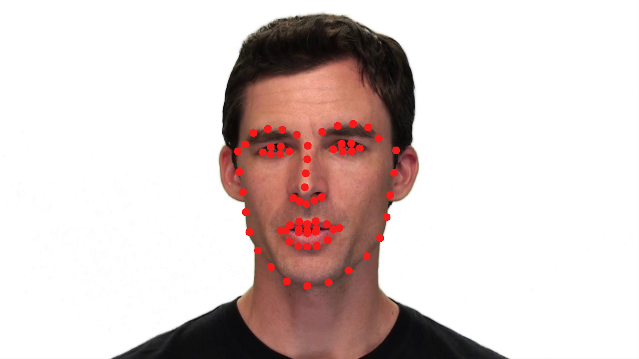
Furthermore, as the associated videos of the audios are available in the RAVDESS dataset, we would like to use the landmarks (see Fig. 6) as input to topological data analysis tools (like a Vietoris-Rips filtration) and combine this information within the one provided by the audios used in this paper. Similarly, one of the most relevant conclusions that KRISTINA project reached was that the combination of visual and audio features can develop better predictions than using them separately.

References

- [1] Anastasiya S. Popova, Alexandr G. Rassadin, and Alexander A. Ponomarenko. Emotion recognition in sound. In Boris Kryzhanovsky, Witali Dunin-Barkowski, and Vladimir Redko, editors, Advances in Neural Computation, Machine Learning, and Cognitive Research, pages 117–124, Cham, 2018. Springer International Publishing.
- [2] Andrew Ortony and Terence J Turner. What’s basic about basic emotions? Psychological review, 97(3):315, 1990.
- [3] J.A. Russell. A circumplex model of affect. Journal of personality and social psychology, 39(6):1161–1178, 1980.
- [4] Dimitrios Ververidis and Constantine Kotropoulos. Emotional speech recognition: resources, features, and methods. Speech Communication, pages 1162–1181, 2006.
- [5] Larry Wasserman. Topological data analysis. Annual Review of Statistics and Its Application, 5(1):501–532, 2018.
- [6] Matteo Rucco, Rocio Gonzalez-Diaz, Maria-Jose Jimenez, Nieves Atienza, Cristina Cristalli, Enrico Concettoni, Andrea Ferrante, and Emanuela Merelli. A new topological entropy-based approach for measuring similarities among piecewise linear functions. Signal Processing, 134:130 – 138, 2017.
- [7] Eitan Globerson, Noam Amir, Ofer Golan, Liat Kishon-Rabin, and Michal Lavidor. Psychoacoustic abilities as predictors of vocal emotion recognition. Attention, Perception, & Psychophysics, 75(8):1799–1810, Nov 2013.
- [8] David M. Howard and James Angus. Acoustics and Psychoacoustics. Butterworth-Heinemann, Newton, MA, USA, 2nd edition, 2000.
- [9] B. Yang and M. Lugger. Emotion recognition from speech signals using new harmony features. Signal Processing, 90(5):1415 – 1423, 2010. Special Section on Statistical Signal & Array Processing.
- [10] B. Schuller and A. Batliner. Computational Paralinguistics: Emotion, Affect and Personality in Speech and Language Processing. Wiley, 2013.
- [11] Herbert Edelsbrunner and John L. Harer. Computational Topology, An Introduction. American Mathematical Society, 2010.
- [12] G.E. Bredon. Topology and Geometry. Springer, New York, 1993.
- [13] A. Zomorodian and G. Carlsson. Computing persistent homology. Discrete and Computational Geometry, 33(2):249–274, 2005.
- [14] Bernhard E. Boser, Isabelle M. Guyon, and Vladimir N. Vapnik. A training algorithm for optimal margin classifiers. In Proceedings of the Fifth Annual Workshop on Computational Learning Theory, COLT ’92, pages 144–152, New York, NY, USA, 1992. ACM.
- [15] Corinna Cortes and Vladimir Vapnik. Support-vector networks. Machine Learning, 20(3):273–297, Sep 1995.
- [16] Nello Cristianini and John Shawe-Taylor. An Introduction to Support Vector Machines and Other Kernel-based Learning Methods. Cambridge University Press, 1 edition, 2000.
- [17] Aurelien Géron. Hands-on machine learning with Scikit-Learn and TensorFlow : concepts, tools, and techniques to build intelligent systems. O’Reilly Media, Sebastopol, CA, 2017.
- [18] Karl Pearson. Note on regression and inheritance in the case of two parents. Proceedings of the Royal Society of London, 58:240–242, 1895.
- [19] Steven R. Livingstone and Frank A. Russo. The ryerson audio-visual database of emotional speech and song (ravdess): A dynamic, multimodal set of facial and vocal expressions in north american english. PLOS ONE, 13(5):1–35, 05 2018.
- [20] Biqiao Zhang, Georg Essl, and Emily Mower Provost. Recognizing emotion from singing and speaking using shared models. In Proceedings of the 2015 International Conference on Affective Computing and Intelligent Interaction (ACII), ACII ’15, pages 139–145, Washington, DC, USA, 2015. IEEE Computer Society.