Neural Generative Models for 3D Faces with Application in 3D Texture Free Face Recognition

Abstract

Using heterogeneous depth cameras and 3D scanners in 3D face verification causes variations in the resolution of the 3D point clouds. To solve this issue, previous studies use 3D registration techniques. Out of these proposed techniques, detecting points of correspondence is proven to be an efficient method given that the data belongs to the same individual. However, if the data belongs to different persons, the registration algorithms can convert the 3D point cloud of one person to another, destroying the distinguishing features between the two point clouds. Another issue regarding the storage size of the point clouds. That is, if the captured depth image contains around 50 thousand points in the cloud for a single pose for one individual, then the storage size of the entire dataset will be in order of giga if not tera bytes. With these motivations, this work introduces a new technique for 3D point clouds generation using a neural modeling system to handle the differences caused by heterogeneous depth cameras, and to generate a new face canonical compact representation. The proposed system reduces the stored 3D dataset size, and if required, provides an accurate dataset regeneration. Furthermore, the system generates neural models for all gallery point clouds and stores these models to represent the faces in the recognition or verification processes. For the probe cloud to be verified, a new model is generated specifically for that particular cloud and is matched against pre-stored gallery model presentations to identify the query cloud. This work also introduces the utilization of Siamese deep neural network in 3D face verification using generated model representations as raw data for the deep network, and shows that the accuracy of the trained network is comparable all published results on Bosphorus dataset.

1 Introduction

Rapid improvements in 3D capturing techniques increased the utilization of 3D face recognition especially when the regular 2D images fail due to lighting and appearance changes. The techniques used for 3D based face recognition have been summarized in (Bowyer et al.,, 2006; Scheenstra et al.,, 2005; Daoudi et al.,, 2013). Relevant studies are explained in the following text.

The work in (Cartoux et al.,, 1989) uses 3D face recognition by segmenting a range image based on principal curvature and finding a plane of bilateral symmetry through the face. This plane is used for pose normalization. The authors consider methods of matching the profile from the plane of symmetry and of matching the face surface. A modified technique proposed in (Lee and Milios,, 1990), where the authors use segment convex regions in the range image based on the sign of the mean and Gaussian curvatures, and create an Extended Gaussian Image (EGI) for each convex region. A match between a region in a probe image and in a gallery image is done by correlating EGIs. A graph matching algorithm incorporating relational constraints is used to establish an overall match of probe image to gallery image. Convex regions are believed to change shape less than other regions in response to changes in facial expression. This gives this approach some ability to cope with changes in facial expression. However, EGIs are not sensitive to change in object size, and hence two similarly shaped differently sized faces will not be distinguishable in this representation. In (Gordon,, 1992) the author begins with a curvature-based segmentation of the face. Then a set of features are extracted that describe both curvature and metric size properties of the face. Thus each face becomes a point in feature space, and matching is done by a nearest-neighbor match in feature space. It is noted that the values of the features used are generally similar for different images of the same face, “except for the cases with large feature detection error, or variation due to expression” (Gordon,, 1992). Instead of working on all face points, in (Nagamine et al.,, 1992) the authors used 3D five feature points only, using these feature points to standardize face pose, and then matching various curves or profiles through the face data. Experiments are performed for sixteen subjects, with ten images per subject. The best recognition rates are found using vertical profile curves that pass through the central portion of the face. Computational requirements were apparently regarded as severe at the time this work was performed, as the authors note that “using the whole facial data may not be feasible considering the large computation and hardware capacity needed” (Nagamine et al.,, 1992). In (Achermann et al.,, 1997) they extend Eigenface and hidden Markov model approaches used for 2D face recognition to work with range images. (Tanaka et al.,, 1998) also perform curvature-based segmentation and represent the face using an Extended Gaussian Image (EGI). Recognition is then performed using a spherical correlation of the EGIs. In (Achermann and Bunke,, 2000) the authors report on a method of 3D face recognition that uses an extension of the Hausdorff distance matching. Again, work in (Hesher et al.,, 2003) explores principal component analysis (PCA) style approaches using different numbers of eigenvectors and image sizes. The image data set used has 6 different facial expressions for each of the 37 subjects. The performance figures reported resulting from using multiple images per subject in the gallery. This effectively gives the probe image more chances to make a correct match, and is known to raise the recognition rate relative to having a single sample per subject in the gallery (Min et al.,, 2003). Registration and correspondence has been used in (Medioni and Waupotitsch,, 2003) to perform 3D face recognition using iterative closest point (ICP) matching of face surfaces. Even though most of the work covered here used 3D shape acquired through a structured-light sensor, this work uses a stereo-based system. The Approach used in (Moreno et al.,, 2003) is 3D face recognition by first performing a segmentation based on Gaussian curvature and then creating a feature vector based on the segmented regions. The authors report results on a dataset of 420 face meshes representing 60 different persons, with some sampling of different expressions and poses for each person. Another research is perform 3D face recognition by locating the nose tip, and then forming a feature vector based on contours along the face at a sequence of depth values (Lee et al.,, 2003). An isometric transformation approach has been used in (Bronstein et al.,, 2003) to analyze 3D face in an attempt to better cope with variation due to facial expression. Rather than performing recognition on the all face as one module, the authors in (Alyuz et al.,, 2008) have performed recognition using registration on separate face parts and uses fusion to come up with a final decision. Moreover, other research as in (Li et al.,, 2011) and (Maes et al.,, 2010) use the high dimensional extracted features, viz. scale invariant feature transform (SIFT, mesh-SIFT) and histograms for both gradient and shapes, from the 3D cloud, and perform the recognition process on them.

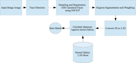
The survey indicates that most if not all research work on extracting some features from given 3D face point clouds and using these features in the recognition process. The extracted features heavily depend on the cloud space and can be easily affected by the structure and size of the given points cloud. These clouds can be modeled to save the storage size or to regenerate the depth information. Other research converts the given 3D points cloud to 2.5D at standard $X$ and $Y$ coordinates using orthographic projection and convert the problem to pixel image recognition as suggested by (Min et al.,, 2012). Figure 1 shows a complete system that uses this technique.

Fig. 1: Example for 3D recognition using registration and projection to 2.5D.

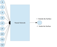
As previously mentioned, there is literature that focus on modeling the 3D face clouds as in (Cretu et al.,, 2006). Here, a neural model is designed as shown in Figure 2. In this network, the input consists of second order values for all input points cloud and the output is 0. Additional input values are added for extra generated surfaces inside and outside the point cloud surface. The output in this case should be proportional to the distance from the input point to the cloud surface as shown in Figure 3. The model however, requires the generation of at least 5 times the number of the original points cloud. Furthermore, the output is not guaranteed to be on the original surface since the acceptance tolerance $d$ is defined for scaling purposes making this model computationally expensive if a higher accuracy required.

Fig. 2: Neural network for 3D points modeling in Cretu et al.

Fig. 3: Extra surfaces generated for neural model learning in Cretu et al.

Despite the fact that there is an increase in the literature that includes Deep-learning and Deep-neural systems in 3D object recognition as in (Richard Socher and Brody Huval and Bharath Bhat and Christopher D. Manning and Andrew Y. Ng,, 2012; Alexandre,, 2016; Nair and Hinton,, 2009), none of these techniques have been applied to 3D face recognition, or it can use the regular 2D representation of the 3D face as in (Kim et al.,, 2017). One reason for this lack of applicability is the high sensitivity and the closeness of features between the faces of different individuals, specifically if the 3D data is used alone without any texture.

Addressing these issues, the main contributions of the proposed 3D neural recognition and verification system are listed as follows.

1. Designing neural generative model for representation and reconstruction of 3D faces,

2. Significantly reducing the storage space used for the 3D point clouds, by replacing the stored point clouds with the generated neural model representations,

3. Using the generated presentation from the 3D regression models of gallery set for recognition and verification against generated model representation for probe points cloud,

4. Combining generated face model representation with Siamese network to generate a comprehensive framework for 3D face verification.

2 Proposed 3D Based Face Recognition System

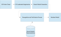
In some cases, due to lighting conditions and/or makeup or other 2D effects in the face image, the regular 2D image becomes insufficient for face recognition. In order to address these issues, this work presents a 3D based face recognition system that is able to work on the texture free 3D point clouds extracted by depth cameras to identify or verify the person. In this regard, this research introduces a new technique for 3D cloud regeneration using a neural generative model to handle the differences caused by heterogeneous depth cameras, and to generate a new face canonical compact representation. The proposed system reduces the stored 3D dataset size and if required, provides an accurate dataset regeneration. Furthermore, the system generates neural models for all gallery point clouds and stores these models to represent these faces in the recognition or verification process. For the probe cloud to be verified, the system obtains the 3D points cloud as an input with face landmark points. These landmark points are then registered to reference points to align and to scale the input cloud correctly. After the registration step, a neural model is generated for this prob cloud to provide a compact representation of the 3D face data. The extracted neural model is then applied to a face recognition or verification step to detect the best matched model from the pre-stored gallery model presentations. This work also introduces the utilization of Siamese deep neural network in 3D face verification using generated model representation as a raw data for the deep network. The complete proposed system is depicted in Figure 4. The following sections will explain each step used in the system.

Fig. 4: Proposed 3D based face recognition system.

3 3D Registration

The first step in the proposed system is the registration that transforms all 3D data into a canonical standard position. This step involves 3D data using Iterative Closest Point (ICP) algorithm. Before applying ICP on the input clouds, these clouds have to be normalized around their means and to be placed inside a cube with maximum dimensions of $2\times 2\times 2$ with each axis having a range $\left[-1,1\right]$. After the normalization step, the landmark points registration is applied to obtain the suitable rigid transformation between input landmark points and the reference points. The output transformation is then applied to all input points to obtain the registered points which will be used in the following steps.

3.1 Iterative Closest Point (ICP)

Iterative Closest Point (ICP), a.k.a., Iterative Corresponding Point, is an algorithm used to obtain the corresponding points and transformations between two groups of points in 2D or 3D. However, the algorithm is mostly used in the 3D cases for registration between some query mesh and standard canonical mesh. The main algorithm was introduced in (Besl and McKay,, 1992). The main goal of (Besl and McKay,, 1992) work is to obtain the optimum transformation matrix $T=\left[R|t\right]$ (where $R$ is the $3\times 3$ rotation matrix and $t$ is $3\times 1$ translation vector) that can convert moving landmark points set $M=\left\{m_{i}\right\}$ to the static points set $S=\left\{s_{i}\right\}$. Assuming that the number of points for both sets are equal ($N_{M}=N_{s}$), the objective function required to be minimized should be

$$f\left(T\right)=\frac{1}{N_{S}}\sum_{i=1}^{N_{s}}\left\|s_{i}-Rm_{i}-t\right\|^{2}.$$ (1)

To achieve this goal the following steps are followed:

1. Starting from iteration $k=0$, $M_{k}=M_{0}=M$

2. Find the closest corresponding points (on Euclidean space) between $M_{k}$ set and $S$ set. These correspondence set will be $Y_{k}=C\left(M_{k},S\right)$.

3. For the particular $Y_{k}$, minimize equation (1) solving for the value of $T$ (using least square techniques). The solution will be $T_{k}$

4. Apply $T_{k}$over $M_{k}$ set to generate $M_{k+1}=R_{k}M_{k}+t_{k}$

5. Set $k=k+1$

6. Repeat steps 2,3 and 4 until the stopping criteria are satisfied.

The main disadvantage of this technique is its computational complexity which reaches to significant levels when the number of points are large ($O\left(N_{m}N_{s}\right)$). However, some research uses other techniques rather than Nearest Neighborhood (NN), which used in step 2, to improve the computation. K-D Tree is one of these alternative algorithms that can be used for this improvement. Other modified versions of ICP have also been introduced to make the algorithm more computationally efficient. As stated in (Rusinkiewicz and Levoy,, 2001) these improvements have been summarized in the following steps:

1. Selecting some set of points in one or both sets.

2. Matching these points to samples in the other set.

3. Weighting the corresponding pairs appropriately.

4. Rejecting certain pairs by looking at each pair individually or considering the entire set of pairs.

5. Assigning an error metric based on the point pairs.

6. Minimizing the error metric.

Based on the new steps, the algorithm will not work on these entire sets, but on some selected samples from both sets. The sampling and rejection steps in the modified algorithm improve the computation complexity, even though this new approach leads to other concerns regarding the best sampling and rejection mechanisms that can be used to obtain the best matching result.

4 Neural Regression Model for 3D Face Representation

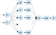
As mentioned previously, one of the problems in the 3D point clouds is the storage size. The storage size for one 3D face including about 80,000 points is in the order of tens if not hundreds of mega bytes. Therefore, finding an alternative representation that can reduce the size while providing the same accuracy is important. An additional concern is th different 3D cameras will produce different cloud resolution (different 3D sensors produce different number of 3D points for the same object). This concern is valid regardless of that the image representing a single person or multiple individuals. To address these issues, a new neural representation is proposed as shown in Figure 5. The proposed neural model will obtain $X$ and $Y$ coordinates as input from the points cloud and will generate the corresponding $\bar{Z}$ values for the same points, which should represent the actual $Z$ values of these points. The mathematical representation of the model will be as the following equations:

$$\bar{Z}^{i}=\tanh\left(n_{f}^{i}\right),$$ (2)

$$n_{f}^{i}=\sum_{j=1}^{M}Wo_{jf}\cdot\tanh\left(n_{j}^{i}\right)+Bo_{f},$$ (3)

$$n_{j}^{i}=\left(Wi_{1j}\cdot X^{i}+Wi_{2j}\cdot Y^{i}\right)+Bi_{j},$$ (4)

where $M$ is the number of hidden units, $\left(X^{i},Y^{i},Z^{i}\right)$ is a 3D point in the point cloud and its corresponding neural output $\bar{Z}^{i}$ and $j$ is the hidden node index.

To obtain the weights $Wi$ and $Wo$ for the neural model, a loss function should be defined and optimized. In this work, the Mean Squared Error (MSE) will be used as stated in equation (5).

$$\mathcal{L}\left(P\right)=\frac{1}{N}\sum_{i=1}^{N}\left\|\bar{Z}^{i}\left(X^{i},Y^{i},P\right)-Z^{i}\right\|{}^{2}.$$ (5)

where $P=\left\{Wi_{1j},Wi_{2j},Bi_{j},Wo_{jf},Bo_{f}\right\}$, $N$ is the number of samples in the points cloud, $Wi_{1,j}$ is the weight of the hidden node $j$ for the first input (the $X$ coordination), $Wi_{2,j}$ is the weight of the hidden node $j$ for the second input (the $Y$ coordination), $Bi_{j}$ is the bias of the hidden node $j$ and $Bo_{f}$ is the bias of the final output node.

To solve this optimization problem, Levenberg–Marquardt Back-Propagation (LM) will be used to obtain the values of $P$ that provides the minimum Mean Squared Error (MSE).

The main advantages of this proposed model are:

• Can be used as a raw data for recognition or verification process: as will be explained and tested in the next sections, the weight matrix $P$ can be flattened (converted to 1D vector) and used as a raw data for verification and recognition.

• Easer in data augmentation (if the model is used as a raw data features for the verification process): in various machine learning problems, the number of available samples for training or testing are limited. To overcome this issue, data augmentation is commonly used to generate additional samples by manipulating the existing data (via shifting, rotating and clipping in the case of image learning). However, in 3D cases, especially for faces, these processes can generate limited number of samples. For the proposed model however, significantly large numbers of new models can be generated for the same face by only swapping rows in the matrix $P$. For example, assuming the structure of the network is 2-500-1 (2 is the number of inputs ($X$ and $Y$ coordinates), $M$ (number of hidden layers) is 500 and 1 output ($Z$ coordinate)), then the size of $Bo_{f}$ will be $1\times 1$ which can be concatenated to the matrix $P$ after flatting it, and the value of $B_{f}$ will not change in all augmented models generated from the original model $P$. So if the original trained model weights $P=P_{1}=\left[\begin{array}[]{cccc}wi_{1,1}&wi_{2,1}&bi_{1}&wo_{1,1}\\ wi_{1,2}&wi_{2,2}&bi_{2}&wo_{2,1}\\ wi_{1,3}&wi_{2,3}&bi_{3}&wo_{3,1}\\ \vdots&\vdots&\vdots&\vdots\\ wi_{1,500}&wi_{2,500}&bi_{500}&wo_{500,1}\end{array}\right]$ then another model $P_{2}=\left[\begin{array}[]{cccc}wi_{1,3}&wi_{2,3}&bi_{3}&wo_{3,1}\\ wi_{1,2}&wi_{2,2}&bi_{2}&wo_{2,1}\\ wi_{1,1}&wi_{2,1}&bi_{1}&wo_{1,1}\\ \vdots&\vdots&\vdots&\vdots\\ wi_{1,500}&wi_{2,500}&bi_{500}&wo_{500,1}\end{array}\right]$ can be generated as a new model that represents the same face as $P_{1}$ by only swapping rows 1 and 3. Therefore, assuming that $M$ equal to 500, this technique can generate $500!$ different models for the same face from a single trained model.

• Reduce the storage size of the face representation: because to store a 3D face only the network weights need to be stored (assuming the network structure is known). For instance, if the network structure is (2-500-1), the number of stored weights will be 2001 (taking into account the network biases). This means that instead of storing about 80,000 double precision numbers or more (the original number of points in the cloud), only 2,000 float precision numbers can be stored which will improve the storage size with a factor of 80.

• Independent of the number of points in the trained cloud: to train the proposed neural model you don’t need specific number of points in the cloud (you can train the model with 80,000, 50,000 or 15,000 points). Which means that the generated model can be trained using different camera’s resolution. This makes this technique suitable for heterogeneous cameras.

• Can be used in 3D super-resolution: the neural generated model designed in this work is a regression model that can be used for smoother accurate interpolation to generate higher resolution version from the original 3D points, which can considered as 3D super-resolution algorithm.

Fig. 5: Proposed neural representation of face depth data .

5 Levenberg–Marquardt Back-Propagation

In the Gradient Decent Back-Propagation algorithm, the back-propagated recurrent form of sensitivity at layer $k$ in the neural network has been formulated as

$$\delta^{k}=\dot{F}^{k}\left(n^{k}\right).W^{k+1^{T}}.\delta^{k+1},$$ (6)

where

$$\dot{F}^{k}\left(n^{k}\right)=\left[\begin{array}[]{cccc}\dot{f}^{k}\left(n^{k}\left(1\right)\right)&0&\cdots&0\\ 0&\dot{f}^{k}\left(n^{k}\left(2\right)\right)&\cdots&0\\ \vdots&\vdots&\ddots&\vdots\\ 0&0&\cdots&\dot{f}^{k}\left(n^{k}\left(S_{k}\right)\right)\end{array}\right],$$ (7)

and

$$\dot{f}^{k}\left(n^{k}\left(i\right)\right)=\frac{df^{k}\left(n^{k}\left(i\right)\right)}{dn^{k}\left(i\right)}.$$ (8)

where $f^{k}\left(n^{k}\left(i\right)\right)$ is the activation function of node $i$ in layer $k$, $n^{k}\left(i\right)$ is the output of node $i$ in layer $k$ and $W$ represents all weights and biases in the network.

The Gradient Decent method works well when the network task is a classification with softmax loss function. However, for some tasks, the loss function is defined as Mean Squared Error (MSE) function between neural network output $a^{M}$and required output $y$. Based on this, the loss function can be defined as

$$e_{i}\left(W\right)=\left(y_{i}-a_{i}^{M}\left(W\right)\right),$$ (9)

$$\mathcal{L}\left(W\right)=\frac{1}{2}\sum_{i=1}^{N}e_{i}^{2}\left(W\right),$$ (10)

where $N=Q\times S_{m}$

Based on Levenberg–Marquardt algorithm used in (Hagan and Menhaj,, 1994), weights and biases update can be calculated as

$$\Delta W=-\left[\nabla^{2}\mathcal{L}\left(W\right)\right]^{-1}\nabla\mathcal{L}\left(W\right),$$ (11)

where $\nabla^{2}\mathcal{L}\left(W\right)$ is the Hessian matrix and $\nabla\mathcal{L}\left(W\right)$is the gradient. The gradient term can be expressed as

$$\nabla\mathcal{L}\left(W\right)=J^{T}\left(W\right)e\left(W\right),$$ (12)

where $e\left(w\right)=\left[\begin{array}[]{c}e_{1}\left(W\right)\\ e_{2}\left(W\right)\\ \vdots\\ e_{N}\left(W\right)\end{array}\right]$, and the Hessian matrix can be approximated as

$$\nabla^{2}\mathcal{L}\left(W\right)=J^{T}\left(W\right)J\left(W\right),$$ (13)

where $J$ is the Jacobian matrix stated as

$$J\left(W\right)=\left[\begin{array}[]{cccc}\frac{\partial e_{1}\left(W\right)}{\partial W_{1}}&\frac{\partial e_{1}\left(W\right)}{\partial W_{2}}&\cdots&\frac{\partial e_{1}\left(W\right)}{\partial W_{n}}\\ \frac{\partial e_{2}\left(W\right)}{\partial W_{1}}&\frac{\partial e_{2}\left(W\right)}{\partial W_{2}}&\cdots&\frac{\partial e_{2}\left(W\right)}{\partial W_{n}}\\ \vdots&\vdots&\ddots&\vdots\\ \frac{\partial e_{N}\left(W\right)}{\partial W_{1}}&\frac{\partial e_{N}\left(W\right)}{\partial W_{2}}&\cdots&\frac{\partial e_{N}\left(W\right)}{\partial W_{n}}\end{array}\right],$$ (14)

From equations (12), (13), (14) and (11) can be expressed as

$$\Delta W=\left[J^{T}\left(W\right)J\left(W\right)\right]^{-1}J^{T}\left(W\right)e\left(W\right),$$ (15)

Adding one more control parameter the update can be stated as

$$\Delta W=\left[J^{T}\left(W\right)J\left(W\right)+\mu I\right]^{-1}J^{T}\left(W\right)e\left(W\right),$$ (16)

The new added parameter $\mu$ is used as a variable step control for the updates based on the loss value. Every time the loss $\mathcal{L}\left(W\right)$ reduces, the value of $\mu$ is divided over some other constant parameter $\beta$ to go closer to the minimum loss value.

Applying the new equation to back-propagation algorithm in section 3 resulting in new weight update equation

$$\Delta w^{k+1}\left(i,j\right)=-\alpha.\frac{\partial L_{q}}{\partial w^{k+1}\left(i,j\right)}=-\alpha.\frac{\partial\sum_{m=1}^{S_{M}}e_{q}^{2}\left(m\right)}{\partial w^{k+1}\left(i,j\right)},$$ (17)

$$\Delta b^{k+1}\left(i\right)=-\alpha.\frac{\partial L_{q}}{\partial b^{k+1}\left(i\right)}=\Delta b^{k+1}\left(i\right)=-\alpha.\frac{\partial\sum_{m=1}^{S_{M}}e_{q}^{2}\left(m\right)}{\partial b^{k+1}\left(i\right)},$$ (18)

Identical steps used in the regular back-propagation can also be used with the LM method to fill the Jacobian matrix with small modification at the final step

$$\delta^{M}=-\dot{F}^{M}\left(n^{M}\right).$$ (19)

Based on these equations, the LM back-propagation algorithm will work as follows:

Apply all $Q$ inputs to the network and calculate network outputs and errors corresponding to these output and loss value.

1. Use equations (19), (8), (7), (6), (14) to calculate Jacobian matrix (other efficient Jacobian calculation methods can be used in this step).

2. Solve equation (16) (using Cholesky factorization) for the $\Delta W$.

3. Use the calculated $\Delta W$ to calculate the new value of $W+\Delta W$.

4. Check the new loss value, if the loss value decrease, then decrease $\mu$ by $\beta$ , update $W=W+\Delta W$ and go to step 1. If the loss didn’t reduce increase $\mu$ by $\beta$ and go to step 3.

5. Repeat the these steps until the stopping criteria are satisfied.

Algorithm 1 Levenberg–Marquardt algorithm

6 Recognition and Verification

Using similarity metric for face verification is proven to be an efficient method, especially if the number of images per class is low. Therefore, this work utilizes the similarity metric method with Convolutional Neural Network (CNN) to perform a Siamese Network that will be applied in the final step of the proposed system to perform the verification process.

Using Siamese Network for face verification has been introduced in (Chopra et al.,, 2005), where two input images $X_{1}$ and $X_{2}$ are applied to the same nonlinear mapping $G_{W}$ to extract the main features that minimize the main energy function $E$ when $X_{1}$ and $X_{2}$ belong to the same person and maximize it when they belong to different persons. The typical structure for this network is shown in Figure 6 (Chopra et al.,, 2005). The formal definition of the function $E$ can be expressed as in equation (20)

$$E\left(W,X_{1},X_{2}\right)=\left\|G_{W}\left(X_{1}\right)-G_{W}\left(X_{2}\right)\right\|,$$ (20)

where $W$ are the shared weight filters between the two input images.

Fig. 6: Typical structure of Siamese network.

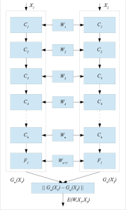
To achieve this goal for the $E$ function, the loss function should monotonically increase with same person pairs’ energy and monotonically decrease with different persons pairs’ energy. Based on this, the final loss function will be formed as in equations (21),(22),(23),(24),(25)

$$\mathcal{L}\left(W\right)=\sum_{i=1}^{N}L\left(W,\left(Y,X_{1},X_{2}\right)^{i}\right),$$ (21)

$$L\left(W,\left(Y,X_{1},X_{2}\right)^{i}\right)=Y\cdot L^{s}\left(E\left(W,X_{1},X_{2}\right)^{i}\right)+\\ \left(1-Y\right)\cdot L^{d}\left(E\left(W,X_{1},X_{2}\right)^{i}\right),$$ (22)

$$L^{s}\left(E\left(W,X_{1},X_{2}\right)^{i}\right)=\frac{2}{Q}\left(E\left(W,X_{1},X_{2}\right)^{i}\right)^{2},$$ (23)

$$L^{d}\left(E\left(W,X_{1},X_{2}\right)^{i}\right)=2Q\cdot e^{\left(-\frac{2.77}{Q}E\left(W,X_{1},X_{2}\right)^{i}\right)},$$ (24)

$$Y=\begin{cases}1&X_{1}\equiv X_{2}\\ 0&X_{1}\not\equiv X_{2}\end{cases}.$$ (25)

where $N$ is the number of training samples, $Y$ is equal to $1$ if $X_{1}$ and $X_{2}$ belong to the same person and $0$ if they present different persons. $L^{s}$ is the loss function in the case of same persons, $L^{d}$ is the loss function in the case of different ones and $Q$ is a constant representing the upper bound of $E$.

Since the energy is monotonically changing for both $L^{s}$ and $L^{d}$, the optimization of the loss function can be easily achieved using simple gradient decent algorithm, and the weights $W$ can be learned using back-propagation algorithm.

The final step of the proposed system involves detecting the identity of the query person or verifying his/her identity. This step utilizes this network structure. For the proposed system, the extracted weights $P$ from the previous section constiture the feature vector used in the recognition or verification process. This means that a 1D Siamese structure network will be used for this verification task. The network structure is depicted in Figure 6. However, $X_{1}$ and $X_{2}$ will be replaced by vectorized $P_{1}$ and $P_{2}$ extracted from the previous step. All calculations stated by equations (20),(21),(22),(23),(24) and (25) will remain identical. However, $W$ will consist of 1D vectors as opposed to 2D as in the original case.

7 Results

The proposed system has been tested over the Bosphorus (Savran et al.,, 2008) database. This dataset consists of 3D and textures for 105 persons with different facial expressions. For this test only the 3D faces with neutral expressions are used to test the efficiency of the proposed neural model. Each person has between 1 to 4 neutral faces with a total of 299 neutral 3D texture free faces each of them has on average 80,000 3D points. The target mean squared error (MSE) value for the trained models is below 0.0002. The network structure for this problem is provided in Figure 7. For the sake of simplicity, only one hidden layer is used in the experiment with the number of nodes in the hidden layer being 500. The proposed neural model has been implemented using Neural Network Toolbox of MATLAB.

Fig. 7: Structure of the network used in the experiment.

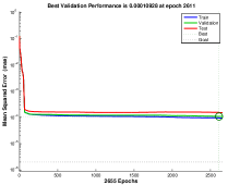
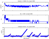
As shown in the sample training in Figure 8, the training loss improved in the first 100 epochs. Following this, all upcoming epochs worked as fine tuner for the learning parameters.

(a)

(b)

Fig. 8: Training performance of one of the generated models.

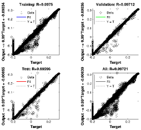
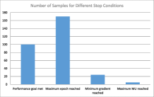
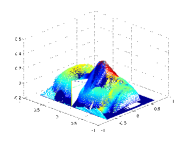
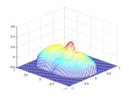
A sample of the resulting regression model accuracy is shown in Figure 9. It can easily be observed that the accuracy of the generated model is more than 99% for presenting target points cloud. Out of all trained models (299 models), 100 models achieved the required training MSE of 0.0002, and 170 models terminated when the maximum number of epochs were reached with an average MSE of 0.00031, which is still considered to be very low error. Also as shown in Figure 10, only few models (29 models) terminated for achieving maximum gradient or maximum $\mu$ value for equation (16). Figure 11 shows a sample of the generated points cloud compared to the original one. As also seen in this figure, the original depth points cloud contains a significantly large noise due to camera and environment. However, the generated points cloud is smoother and provides better view of 3D faces.

Fig. 9: Regression result for one of the generated model.

Fig. 10: Number of training models and their stop conditions.

(a)

(b)

Fig. 11: Sample of original depth points cloud (a) and points cloud generated by regression model (b).

(a)

(b)

(c)

Fig. 12: (a) Training loss of the Siamese Network over 50000 iterations and (b) testing loss of the Siamese Network and (c) testing accuracy of the same network for verification.

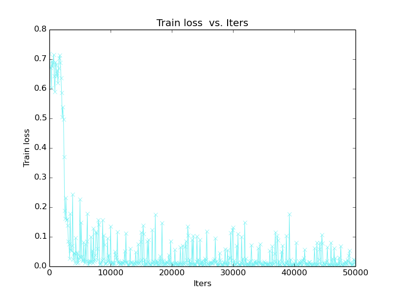
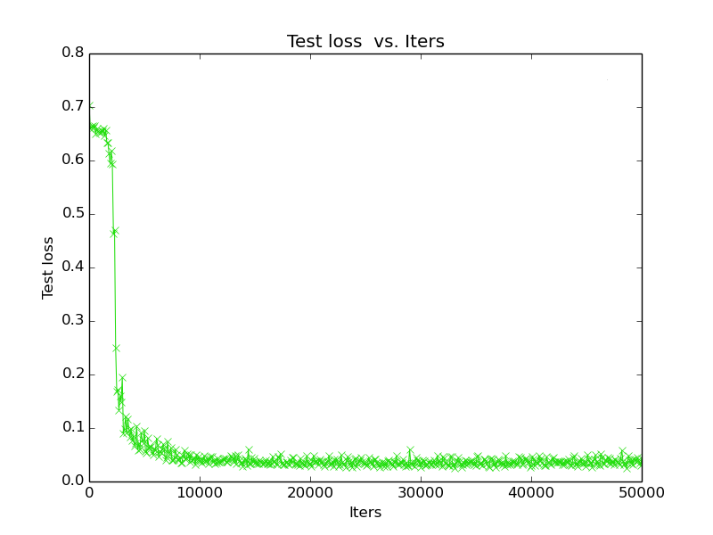
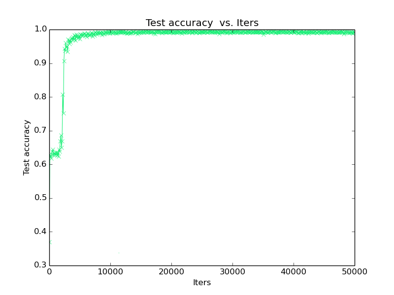
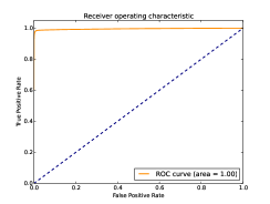
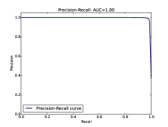
A Siamese network followed by a verification system has been implemented using Caffe library with Python wrapper. The structure of the this network is shown in Figure 13. The 299 neural models which are generated for the 105 persons have been used for training and testing. Randomly selected pairs from the generated models have been selected as a positive (pairs for the same person) and negative (pairs for different persons) training data for the Siamese network. Since the number of positive samples are so limited, the data augmentation technique proposed in section 4 has been used to generate additional pairs for the training and testing. Using this data augmenting technique, the number of generated samples for same person class (positive pairs) is 50,000 samples and for different person class (negative pairs) is 70,000 samples. In the training phase only 50% of the generated pairs (50% of the positive pairs and 50% of the negative ones) are used and the remaining 50% of the data are used for testing. As it can be seen from Figure 12, the loss function of the trained network did not over-fit, and the network is efficiently trained. The accuracy of the trained network over training pairs achieved 100% and 100% for testing pairs. The receiver operation characteristic (ROC) and Precision-Recall curves for the trained network over the testing pairs are also shown in Figure 14. As also provided in Table 1, the achieved verification performance is comparable to the state-of-the-art results published on the same dataset on the neutral expression faces. These techniques include ICP, Average Regional Models (ARMs), Histogram of Gradient (HoG), Histogram of Shape index (HoS), Histogram of Gradient Shape index (HoGS) and the fusion of these histograms (HoG+HoS+HoGS). Once again, these generated neural models for these faces can regenerate the 3D point clouds again to be utilized with any of these mentioned recognition techniques, which give the proposed model more flexibility if the user want to use or develop different algorithm.

Fig. 13: Proposed Siamese network structure.

(a)

(b)

Fig. 14: (a) ROC curve of the Siamese network over testing data and (b) Precision-Recall curve for the same network on the same data.

Method	Rate (%)
ICP-based holistic approach (Alyuz et al.,, 2008)	71.39
Average Regional Models (ARMs) (Alyuz et al.,, 2008)	98.87
HoG+HoS+HoGS (Li et al.,, 2011)	99.98
proposed Siamese Network	100

Table 1: Comparison of recognition rate using different techniques over 3D neutral expression faces of Bosporus dataset.

8 Conclusions

In this work, a neural generative modeling technique for texture free 3D faces has been proposed. The neural models have been used for presentation and regeneration of the 3D faces. The proposed models have been proven to be accurate representations of the original 3D point clouds with additional benefits such as reduced 3D cloud storage size, and their ability to accommodate interpolation and 3D super-resolution. One other advantage of these models is the flexibility of training from different number of points in the cloud, which makes them suitable for heterogeneous cameras. The weights of the trained models have been used as a raw data with Siamese CNN network for a complete neural 3D face recognition and verification system. These weights have advantage over the regular 3D clouds for data augmentation. Furthermore, they allow generation of additional models from a given single model, which makes this technique advantageous for small dataset recognition given that one of the limitations of using CNN that it required large dataset for training and validation. The Siamese network has been trained over the generated pairs (positive and negative) from the trained models. The results obtained from the trained Siamese network outperformed all reported results over the Bosporus dataset for the neutral 3D faces.

References

- Achermann and Bunke, (2000) Achermann, B. and Bunke, H. (2000). Classifying range images of human faces with hausdorff distance. In 2000. Proceedings. 15th International Conference on Pattern Recognition,, volume 2, pages 809–813 vol.2.
- Achermann et al., (1997) Achermann, B., Jiang, X., and Bunke, H. (1997). Face recognition using range images. In Proceedings., International Conference on Virtual Systems and MultiMedia, 1997. VSMM ’97., pages 129–136.
- Alexandre, (2016) Alexandre, L. (2016). 3d object recognition using convolutional neural networks with transfer learning between input channels. In Menegatti, E., Michael, N., Berns, K., and Yamaguchi, H., editors, Intelligent Autonomous Systems 13, volume 302 of Advances in Intelligent Systems and Computing, pages 889–898. Springer International Publishing.
- Alyuz et al., (2008) Alyuz, N., Gokberk, B., and Akarun, L. (2008). A 3d face recognition system for expression and occlusion invariance. In 2008 IEEE Second International Conference on Biometrics: Theory, Applications and Systems, pages 1–7.
- Besl and McKay, (1992) Besl, P. J. and McKay, N. D. (1992). A method for registration of 3-d shapes. IEEE Trans. Pattern Anal. Mach. Intell., 14(2):239–256.
- Bowyer et al., (2006) Bowyer, K. W., Chang, K., and Flynn, P. (2006). A survey of approaches and challenges in 3d and multi-modal 3d + 2d face recognition. Comput. Vis. Image Underst., 101(1):1–15.
- Bronstein et al., (2003) Bronstein, A. M., Bronstein, M. M., and Kimmel, R. (2003). Expression-invariant 3d face recognition. In Kittler, J. and Nixon, M. S., editors, AVBPA, volume 2688 of Lecture Notes in Computer Science, pages 62–69. Springer.
- Cartoux et al., (1989) Cartoux, J. Y., LaPreste, J. T., and Richetin, M. (1989). Face authentication or recognition by profile extraction from range images. In Proceedings of the Workshop on Interpretation of 3D Scenes, pages 194–199.
- Chopra et al., (2005) Chopra, S., Hadsell, R., and LeCun, Y. (2005). Learning a similarity metric discriminatively, with application to face verification. In CVPR 2005. IEEE Computer Society Conference on Computer Vision and Pattern Recognition, 2005., volume 1, pages 539–546 vol. 1.
- Cretu et al., (2006) Cretu, A.-M., Petriu, E., and Patry, G. (2006). Neural-network-based models of 3-d objects for virtualized reality: a comparative study. IEEE Transactions on Instrumentation and Measurement,, 55(1):99–111.
- Daoudi et al., (2013) Daoudi, M., Srivastava, A., and Veltkamp, R. (2013). 3D Face Modeling, Analysis and Recognition. Wiley Publishing, 1st edition.
- Gordon, (1992) Gordon, G. (1992). Face recognition based on depth and curvature features. In Proceedings CVPR ’92., 1992 IEEE Computer Society Conference on Computer Vision and Pattern Recognition, 1992., pages 808–810.
- Hagan and Menhaj, (1994) Hagan, M. and Menhaj, M. (1994). Training feedforward networks with the marquardt algorithm. IEEE Transactions on Neural Networks,, 5(6):989–993.
- Hesher et al., (2003) Hesher, C., Srivastava, A., and Erlebacher, G. (2003). A novel technique for face recognition using range imaging. In Proceedings. Seventh International Symposium on Signal Processing and Its Applications, 2003., volume 2, pages 201–204 vol.2.
- Kim et al., (2017) Kim, D., Hernandez, M., Choi, J., and Medioni, G. (2017). Deep 3d face identification. In 2017 IEEE International Joint Conference on Biometrics (IJCB), pages 133–142.
- Lee and Milios, (1990) Lee, J. and Milios, E. (1990). Matching range images of human faces. In Proceedings, Third International Conference on Computer Vision, 1990., pages 722–726.
- Lee et al., (2003) Lee, Y., Park, K., Shim, J., and Yi, T. (2003). 3d face recognition using statistical multiple features for the local depth information. In 16th International Conference on Vision Interface.
- Li et al., (2011) Li, H., Huang, D., Lemaire, P., Morvan, J. M., and Chen, L. (2011). Expression robust 3d face recognition via mesh-based histograms of multiple order surface differential quantities. In 2011 18th IEEE International Conference on Image Processing, pages 3053–3056.
- Maes et al., (2010) Maes, C., Fabry, T., Keustermans, J., Smeets, D., Suetens, P., and Vandermeulen, D. (2010). Feature detection on 3d face surfaces for pose normalisation and recognition. In 2010 Fourth IEEE International Conference on Biometrics: Theory, Applications and Systems (BTAS), pages 1–6.
- Medioni and Waupotitsch, (2003) Medioni, G. and Waupotitsch, R. (2003). Face recognition and modeling in 3d. In IEEE International Workshop on Analysis and Modeling of Faces and Gestures (AMFG 2003), pages 232–233.
- Min et al., (2003) Min, J., Bowyer, K. W., and Flynn, P. (2003). Using multiple gallery and probe images per person to improve performance of face recognition. Technical report, Notre Dame Computer Science and Engineering Technical Report.
- Min et al., (2012) Min, R., Choi, J., Medioni, G., and Dugelay, J. (2012). Real-time 3d face identification from a depth camera. In 2012 21st International Conference on Pattern Recognition (ICPR),, pages 1739–1742.
- Moreno et al., (2003) Moreno, A. B., Ángel Sánchez, Vélez, J. F., and Díaz, F. J. (2003). Face recognition using 3d surface-extracted descriptors. In In Irish Machine Vision and Image Processing Conference (IMVIP 2003), Sepetember.
- Nagamine et al., (1992) Nagamine, T., Uemura, T., and Masuda, I. (1992). 3d facial image analysis for human identification. In Proceedings., 11th IAPR International Conference on Pattern Recognition, 1992. Vol.I. Conference A: Computer Vision and Applications,, pages 324–327.
- Nair and Hinton, (2009) Nair, V. and Hinton, G. E. (2009). 3d object recognition with deep belief nets. In Bengio, Y., Schuurmans, D., Lafferty, J., Williams, C., and Culotta, A., editors, Advances in Neural Information Processing Systems 22, pages 1339–1347. Curran Associates, Inc.
- Richard Socher and Brody Huval and Bharath Bhat and Christopher D. Manning and Andrew Y. Ng, (2012) Richard Socher and Brody Huval and Bharath Bhat and Christopher D. Manning and Andrew Y. Ng (2012). Convolutional-Recursive Deep Learning for 3D Object Classification. In Advances in Neural Information Processing Systems 25.
- Rusinkiewicz and Levoy, (2001) Rusinkiewicz, S. and Levoy, M. (2001). Efficient variants of the ICP algorithm. In Third International Conference on 3D Digital Imaging and Modeling (3DIM).
- Savran et al., (2008) Savran, A., Alyüz, N., Dibeklioğlu, H., Çeliktutan, O., Gökberk, B., Sankur, B., and Akarun, L. (2008). Biometrics and identity management. chapter Bosphorus Database for 3D Face Analysis, pages 47–56. Springer-Verlag, Berlin, Heidelberg.
- Scheenstra et al., (2005) Scheenstra, A., Ruifrok, A., and Veltkamp, R. (2005). A survey of 3d face recognition methods. In Kanade, T., Jain, A., and Ratha, N., editors, Audio- and Video-Based Biometric Person Authentication, volume 3546 of Lecture Notes in Computer Science, pages 891–899. Springer Berlin Heidelberg.
- Tanaka et al., (1998) Tanaka, H., Ikeda, M., and Chiaki, H. (1998). Curvature-based face surface recognition using spherical correlation. principal directions for curved object recognition. In Proceedings. Third IEEE International Conference on Automatic Face and Gesture Recognition, 1998., pages 372–377.