Voronoi Partition-based Scenario Reduction for Fast Sampling-based Stochastic Reachability Computation of LTI Systems

Hossein Sartipizadeh, Abraham P. Vinod, Behçet Açıkmeşe, and Meeko Oishi This material is based upon work supported by the National Science Foundation, the Air Force Office of Scientific Research, and the Office of Naval Research. Hossein Sartipizadeh and Behçet Açıkmeşe were supported by Air Force Research Laboratory grant FA8650-15-C-2546 and the Office of Naval Research (ONR) Grant No. N00014-15-IP-00052. Vinod and Oishi were supported under NSF Grant Number CMMI-1254990, NSF Grant No. IIS-1528047, and AFRL Grant No. FA9453-17-C-0087. Any opinions, findings, and conclusions or recommendations expressed in this material are those of the authors and do not necessarily reflect the views of the National Science Foundation.
H. Sartipizadeh (corresponding author) is with University of Texas at Austin, TX, US. Email: hsartipi@utexas.edu.
A. Vinod and M. Oishi are with the Electrical & Computer Engineering, University of New Mexico, Albuquerque, NM, US. Email: aby.vinod@gmail.com; oishi@unm.edu.
B. Açıkmeşe is with the Department of Aeronautics & Astronautics in the University of Washington, Seattle, WA. Email: behcet@uw.edu.
Abstract

In this paper, we address the stochastic reach-avoid problem for linear systems with additive stochastic uncertainty. We seek to compute the maximum probability that the states remain in a safe set over a finite time horizon and reach a target set at the final time. We employ sampling-based methods and provide a lower bound on the number of scenarios required to guarantee that our estimate provides an underapproximation. Due to the probabilistic nature of the sampling-based methods, our underapproximation guarantee is probabilistic, and the proposed lower bound can be used to satisfy a prescribed probabilistic confidence level. To decrease the computational complexity, we propose a Voronoi partition-based to check the reach-avoid constraints at representative partitions (cells), instead of the original scenarios. The state constraints arising from the safe and target sets are tightened appropriately so that the solution provides an underapproximation for the original sampling-based method. We propose a systematic approach for selecting these representative cells and provide the flexibility to trade-off the number of cells needed for accuracy with the computational cost.

1 Introduction

Reach-avoid analysis is an established verification tool for discrete-time stochastic dynamical systems, which provides probabilistic guarantees on the safety and performance [1, 2, 3, 4, 5]. This paper focuses on the finite time horizon terminal hitting time stochastic reach-avoid problem [1] (referred to here as the terminal time problem), that is, computation of the maximum probability of hitting a target set at the terminal time, while avoiding an unsafe set during all the preceding time steps using a controller that satisfies the specified control bounds.

The solution to the terminal time problem relies on dynamic programming [1, 6, 7], hence a variety of approximation methods have been suggested in literature. Researchers have looked for scalable approaches to solve this problem using approximate dynamic programming [8, 9], Gaussian mixtures [8], particle filters [9, 4], convex chance-constrained optimization [4], Fourier transform-based verification [10, 11], Lagrangian approaches [5], and semi-definite programming [12]. Currently, the largest system verified is a 404040-dimensional chain of double integrators [10, 11] using Fourier transform-based techniques. Existing methods impose a high computational complexity which makes them unrealistic for real-time applications.

In this paper, we reconsider the sampling-based approach, proposed in [4]. Similar sampling-based approach has been used successfully in robotics [13] and in stochastic optimal control [14, 15, 16, 17]. In the sampling-based stochastic reach-avoid problem, we sample the stochastic disturbance to produce a finite set of scenarios, and then formulate a mixed-integer linear program (MILP) to maximize the number of scenarios that satisfy the reach-avoid constraints [13, 4]. As expected, the approximated probability will converge to the true terminal time probability as the number of scenarios increases. However, the computational complexity of MILP increases exponentially with the number of binary decision variables (the number of scenarios) [18, Rem. 1] making the MILP formulation practically intractable.

The main contributions of this paper are two-fold. We first provide a lower bound on the number of scenarios needed to probabilistically guarantee a user-specified upper bound on the approximation error with a user-specified confidence level using concentration techniques. Using Hoeffding’s inequality, we demonstrate that the number of scenarios that need to be considered is inversely proportional to the square of the desired upper bound on the estimate error. Next, we propose a Voronoi-based undersampling technique that underapproximates the MILP-based solution in a computationally efficient manner. This approach allows us to partially mitigate the exponential computational complexity, and provides flexibility to select the number of partitions based on the allowable online computational complexity. We demonstrate the application of the proposed method in a problem of spacecraft rendezvous and docking.

The organization of the paper is as follows: Problem formulation and preliminary definitions are stated in Section 2. Lower bound on the required number of scenarios for the prescribed confidence level is given in Section 3. Section 4 presents the proposed partition-based method and the approximate solution reconstruction. The performance of the proposed method is investigated on a spacecraft rendezvous maneuvering and docking in Section 5.

2 Problem formulation

We presume \mathbb{R} and \mathbb{N} are sets of real and natural numbers, with nsuperscript𝑛\mathbb{R}^{n} a length n𝑛n vector of real numbers, and [a,b]subscript𝑎𝑏\mathbb{N}_{[a,b]} the set of natural numbers between a𝑎a and b𝑏b. For xn𝑥superscript𝑛x\in\mathbb{R}^{n}, xsuperscript𝑥topx^{\top} denotes the transpose of x𝑥x. Vector with all elements 1 is denoted 𝟏1\mathbf{1}.

2.1 System description

Consider a discrete-time stochastic LTI system,

xt+1=Axt+But+wtsubscript𝑥𝑡1𝐴subscript𝑥𝑡𝐵subscript𝑢𝑡subscript𝑤𝑡x_{t+1}=Ax_{t}+Bu_{t}+w_{t} (1)

with state xt𝒳=nxsubscript𝑥𝑡𝒳superscriptsubscript𝑛𝑥x_{t}\in\mathcal{X}=\mathbb{R}^{n_{x}}, input ut𝒰nusubscript𝑢𝑡𝒰superscriptsubscript𝑛𝑢u_{t}\in\mathcal{U}\subseteq\mathbb{R}^{n_{u}}, disturbance wt𝒲nxsubscript𝑤𝑡𝒲superscriptsubscript𝑛𝑥w_{t}\in\mathcal{W}\subseteq\mathbb{R}^{n_{x}} at time instant t𝑡t, and matrices A,B𝐴𝐵A,B assumed to be of appropriate dimensions. We assume that wksubscript𝑤𝑘w_{k} is an independent and identically distributed (i.i.d) random variable with a PDF ηwsubscript𝜂𝑤\eta_{w}. Note that we require ηwsubscript𝜂𝑤\eta_{w} only to be a probability density function from which we can draw samples, and do not require it to be Gaussian. The system (1) over a time horizon with length N𝑁N can be alternatively written in a “stacked” form,

X(x0,U,W)=Gxx0+GuU+GwW,𝑋subscript𝑥0𝑈𝑊subscript𝐺𝑥subscript𝑥0subscript𝐺𝑢𝑈subscript𝐺𝑤𝑊X(x_{0},U,W)=G_{x}x_{0}+G_{u}U+G_{w}W, (2)

with X=[x1,,xN]𝒳N𝑋superscriptsuperscriptsubscript𝑥1topsuperscriptsubscript𝑥𝑁toptopsuperscript𝒳𝑁X=[x_{1}^{\top},\cdots,x_{N}^{\top}]^{\top}\in\mathcal{X}^{N}, U=[u0,,uN1]𝒰N𝑈superscriptsuperscriptsubscript𝑢0topsuperscriptsubscript𝑢𝑁1toptopsuperscript𝒰𝑁U=[u_{0}^{\top},\cdots,u_{N-1}^{\top}]^{\top}\in\mathcal{U}^{N}, and W=[w0,,wN1]𝒲N𝑊superscriptsuperscriptsubscript𝑤0topsuperscriptsubscript𝑤𝑁1toptopsuperscript𝒲𝑁W=[w_{0}^{\top},\cdots,w_{N-1}^{\top}]^{\top}\in\mathcal{W}^{N} the concatenated state, input, and disturbance vectors over a N𝑁N-length horizon [15]. The matrices Gxsubscript𝐺𝑥G_{x}, Gusubscript𝐺𝑢G_{u}, and Gwsubscript𝐺𝑤G_{w} may be obtained from the system matrices in (1) (see [15]). Due to the stochastic nature of wksubscript𝑤𝑘w_{k}, the state xksubscript𝑥𝑘x_{k} and the concatenated state vector X𝑋X are random. We define Xx0,Usuperscriptsubscript𝑋subscript𝑥0𝑈\mathbb{P}_{X}^{x_{0},U} as the probability measure associated with the random vector X𝑋X, which is induced from the probability measure of the concatenated disturbance vector Wsubscript𝑊\mathbb{P}_{W} and (2). By the i.i.d. assumption on wksubscript𝑤𝑘w_{k}, Wsubscript𝑊\mathbb{P}_{W} is characterized by (ηw)Nsuperscriptsubscript𝜂𝑤𝑁(\eta_{w})^{N}.

2.2 Stochastic reach-avoid problem

We are interested in the terminal time problem [1]. As in [1], we seek open-loop control laws, to assure tractability (at the cost of conservativeness [10, 4, 11]). We define the terminal time probability, rx0U(𝒮,𝒯)superscriptsubscript𝑟subscript𝑥0𝑈𝒮𝒯r_{x_{0}}^{U}(\mathcal{S},\mathcal{T}), for a given initial state x0𝒳subscript𝑥0𝒳x_{0}\in\mathcal{X} and an open-loop control U𝒰N𝑈superscript𝒰𝑁U\in\mathcal{U}^{N}, as the probability that the state trajectory remains inside the safety set 𝒮𝒳𝒮𝒳\mathcal{S}\subseteq\mathcal{X} and reaches the target set 𝒯𝒳𝒯𝒳\mathcal{T}\subseteq\mathcal{X} at time N𝑁N,

rx0U(𝒮,𝒯)superscriptsubscript𝑟subscript𝑥0𝑈𝒮𝒯\displaystyle r_{x_{0}}^{U}(\mathcal{S},\mathcal{T}) =Xx0,U{xN𝒯xt𝒮,t[0,N1]}=Xx0,U{X}1𝒮(x0).\displaystyle=\mathbb{P}_{X}^{x_{0},U}\left\{x_{N}\in\mathcal{T}\wedge x_{t}\in\mathcal{S},\forall t\in\mathbb{N}_{[0,N-1]}\right\}=\mathbb{P}_{X}^{x_{0},U}\left\{X\in\mathcal{R}\right\}1_{\mathcal{S}}(x_{0}). (3)

with =𝒮N1×𝒯superscript𝒮𝑁1𝒯\mathcal{R}=\mathcal{S}^{N-1}\times\mathcal{T}. The stochastic reach-avoid problem is formulated as:

Problem 1.

Open-loop terminal time problem: {maxi} —s— UU^Nr_x_0^U(S, T) p^( x_0)= Problem 1 is equivalent to (see [1, Sec. 4]), {maxi} —s— UU^N1_S( x_0)E_z^x_0,U[ z ],p^( x_0)= where z=1𝒯(xN)t=1N11𝒮(xt)=1(X)𝑧subscript1𝒯subscript𝑥𝑁superscriptsubscriptproduct𝑡1𝑁1subscript1𝒮subscript𝑥𝑡subscript1𝑋z=1_{\mathcal{T}}(x_{N})\prod_{t=1}^{N-1}1_{\mathcal{S}}(x_{t})=1_{\mathcal{R}}(X) is a Bernoulli random variable with a discrete probability measure zx0,Usuperscriptsubscript𝑧subscript𝑥0𝑈\mathbb{P}_{z}^{x_{0},U} induced from Xx0,Usuperscriptsubscript𝑋subscript𝑥0𝑈\mathbb{P}_{X}^{x_{0},U}.

Remark 1.

In Problem 1, p(x0)superscript𝑝subscript𝑥0p^{\ast}(x_{0}) is trivially zero when x0𝒮subscript𝑥0𝒮x_{0}\not\in\mathcal{S}, irrespective of the choice of the controller.

In [4, 13], a mixed-integer linear program (MILP) was formulated as an approximation of Problem 1 when the safe and the target sets are polytopic. Note that restriction of the safe and the target sets to polytopes is not severe since convex and compact sets admit tight polytopic underapproximations [19, Ex. 2.25]. We will denote the safe set 𝒮𝒮\mathcal{S}, the target set 𝒯𝒯\mathcal{T}, and the reach-avoid constraint set \mathcal{R} as

𝒮𝒮\displaystyle\mathcal{S} ={x|f𝒮xh𝒮},absentconditional-set𝑥subscript𝑓𝒮𝑥subscript𝒮\displaystyle=\{x|f_{\mathcal{S}}x\leq h_{\mathcal{S}}\}, (4a)
𝒯𝒯\displaystyle\mathcal{T} ={x|f𝒯xh𝒯},absentconditional-set𝑥subscript𝑓𝒯𝑥subscript𝒯\displaystyle=\{x|f_{\mathcal{T}}x\leq h_{\mathcal{T}}\}, (4b)
\displaystyle\mathcal{R} ={x|FXh}absentconditional-set𝑥𝐹𝑋\displaystyle=\{x|FX\leq h\} (4c)

with l𝒮,l𝒯,L=(N1)l𝒮+l𝒯,f𝒮l𝒮×nxformulae-sequencesubscript𝑙𝒮subscript𝑙𝒯formulae-sequence𝐿𝑁1subscript𝑙𝒮subscript𝑙𝒯subscript𝑓𝒮superscriptsubscript𝑙𝒮subscript𝑛𝑥l_{\mathcal{S}},l_{\mathcal{T}}\in\mathbb{N},L=(N-1)l_{\mathcal{S}}+l_{\mathcal{T}},f_{\mathcal{S}}\in\mathbb{R}^{l_{\mathcal{S}}\times n_{x}}, f𝒯l𝒯×nxsubscript𝑓𝒯superscriptsubscript𝑙𝒯subscript𝑛𝑥f_{\mathcal{T}}\in\mathbb{R}^{l_{\mathcal{T}}\times n_{x}}, and FL×nx𝐹superscript𝐿subscript𝑛𝑥F\in\mathbb{R}^{L\times n_{x}} is constructed using f𝒮subscript𝑓𝒮f_{\mathcal{S}} and f𝒯subscript𝑓𝒯f_{\mathcal{T}}. Using the “big-M” approach [18, 13, 4], and a sampling-based empirical mean for rx0U(𝒮,𝒯)superscriptsubscript𝑟subscript𝑥0𝑈𝒮𝒯r_{x_{0}}^{U}(\mathcal{S},\mathcal{T}) that replaces 𝒲Nsuperscript𝒲𝑁\mathcal{W}^{N} by a finite set of K𝐾K random samples,

𝒲K={W(1),,W(K)},subscript𝒲𝐾superscript𝑊1superscript𝑊𝐾\mathcal{W}_{K}=\{W^{(1)},\cdots,W^{(K)}\}, (5)

we obtain a MILP approximation to Problem 1.

Problem 2.

A MILP approximation to Problem 1 is given by {maxi*}—s— UU^N1K_i=1^Kz^(i)\addConstraintX^(i)= G_xx_0 + G_u U + G_wW^(i), iN_[1,K] \addConstraintFX^(i)h + M(1-z^(i))1, iN_[1,K] \addConstraintz^(i)∈{0,1}, iN_[1,K] with the optimal value denoted by pK(x0)superscriptsubscript𝑝𝐾subscript𝑥0p_{K}^{\ast}(x_{0}), optimal control input UKsubscriptsuperscript𝑈𝐾U^{\ast}_{K}, M𝑀M\in\mathbb{R} some large positive number, and W(i)superscript𝑊𝑖W^{(i)} that are concatenated disturbance realizations sampled from 𝒲Nsuperscript𝒲𝑁\mathcal{W}^{N}, based on the probability law Wsubscript𝑊\mathbb{P}_{W}.

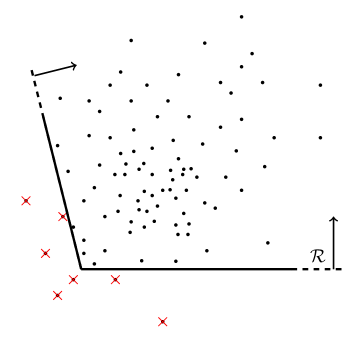
As observed in [4, 18, 13], z(i)superscript𝑧𝑖z^{(i)} takes the value 111 if and only if FX(i)h𝐹superscript𝑋𝑖FX^{(i)}\leq h for all i[1,K]𝑖subscript1𝐾i\in\mathbb{N}_{[1,K]}. For any sampled trajectory that violates the reach-avoid constraint X(j),j[1,K]formulae-sequencesuperscript𝑋𝑗𝑗subscript1𝐾X^{(j)}\in\mathcal{R},\ j\in\mathbb{N}_{[1,K]}, we have FX(j)>h𝐹superscript𝑋𝑗FX^{(j)}>h which is encoded by z(j)=0superscript𝑧𝑗0z^{(j)}=0 . This concept is illustrated in Figure 1; red crosses indicate the sampled trajectories which fail to remain in \mathcal{R} and, therefore, their corresponding binary variables are zero. From [4], we have,

limKpK(x0)=p(x0).subscript𝐾superscriptsubscript𝑝𝐾subscript𝑥0superscript𝑝subscript𝑥0\displaystyle\lim_{{K\rightarrow\infty}}p_{K}^{\ast}(x_{0})=p^{\ast}(x_{0}). (6)

However, Problem 2 becomes computationally intractable for large values of K𝐾K since the worst-case time complexity of MILP problems exponentially increases in the number of binary decision variables [18, Rem. 1].
Refer to caption
Figure 1: Sampling-based approach illustration for reach-avoid problem in 222D. Reach-avoid set \mathcal{R} is distinguished with lines. Black dots and red crosses represent the sampled state trajectories corresponding to sampled disturbance 𝒲Ksubscript𝒲𝐾\mathcal{W}_{K} for a given U𝑈U and x0subscript𝑥0x_{0} that succeed and fail to remain in \mathcal{R}, respectively. Empirical mean of remaining in reach-avoid set is obtained by dividing the number of samples inside \mathcal{R} to the total number of samples.

2.3 Problem statements

Based on Problem 2, we define the random vector Z=[z(1)z(K)]𝑍superscriptdelimited-[]superscript𝑧1superscript𝑧𝐾topZ={[z^{(1)}\ \ldots\ z^{(K)}]}^{\top}, the concatenation of an i.i.d process consisting of Bernoulli random variables {z(i)}i=1Ksuperscriptsubscriptsuperscript𝑧𝑖𝑖1𝐾\{z^{(i)}\}_{i=1}^{K}. By definition, the probability measure associated with Z𝑍Z is Zx0,U=i=1Kzx0,Usuperscriptsubscript𝑍subscript𝑥0𝑈superscriptsubscriptproduct𝑖1𝐾superscriptsubscript𝑧subscript𝑥0𝑈\mathbb{P}_{Z}^{x_{0},U}=\prod_{i=1}^{K}\mathbb{P}_{z}^{x_{0},U}.

We will address the following questions:

Question 1.

Given a violation parameter δ[0,1]𝛿01\delta\in[0,1] and a risk of failure β[0,1]𝛽01\beta\in[0,1], characterize the sufficient number of scenarios K𝐾K to guarantee Zx0,UK{pK(x0)p(x0)δ}βsuperscriptsubscript𝑍subscript𝑥0subscriptsuperscript𝑈𝐾superscriptsubscript𝑝𝐾subscript𝑥0superscript𝑝subscript𝑥0𝛿𝛽\mathbb{P}_{Z}^{x_{0},U^{\ast}_{K}}\{p_{K}^{\ast}(x_{0})-p^{\ast}(x_{0})\geq\delta\}\leq\beta or equivalently Zx0,UK{p(x0)pK(x0)δ}1βsuperscriptsubscript𝑍subscript𝑥0subscriptsuperscript𝑈𝐾superscript𝑝subscript𝑥0superscriptsubscript𝑝𝐾subscript𝑥0𝛿1𝛽\mathbb{P}_{Z}^{x_{0},U^{\ast}_{K}}\{p^{\ast}(x_{0})\geq p_{K}^{\ast}(x_{0})-\delta\}\geq 1-\beta, for all x0𝒮subscript𝑥0𝒮x_{0}\in\mathcal{S}.

Question 2.

Given K𝐾K scenarios as characterized in Question 1 to meet desired specifications, construct an under-approximate MILP with K^<K^𝐾𝐾\hat{K}<K scenarios (hence binary decision variables) that results in the terminal time probability estimate p^(x0)^𝑝subscript𝑥0\hat{p}(x_{0}) with p^(x0)pK(x0)^𝑝subscript𝑥0superscriptsubscript𝑝𝐾subscript𝑥0\hat{p}(x_{0})\leq p_{K}^{\ast}(x_{0}).

We will address Question 1 using Hoeffding’s inequality. By solving Question 1, we seek sufficient number of scenarios that leads to a desired upper bound on the likelihood that the approximate solution exceeds the true solution by some threshold (δ𝛿\delta). Note that a smaller δ𝛿\delta implies less conservatism as well as higher accuracy in estimation, but requires more scenarios for a fixed β𝛽\beta, as claimed in next section. Then we address Question 2 using Voronoi partitions to reduce the number of scenarios while preserving the original specifications δ𝛿\delta and β𝛽\beta.

2.4 Voronoi partition and data clustering

Here we introduce some preliminaries on Voronoi partition that we will use in the rest of this paper. Given a set of seeds (centres) 𝒞={c(1),,c(K^)}𝒞superscript𝑐1superscript𝑐^𝐾\mathcal{C}=\left\{c^{(1)},\cdots,c^{(\hat{K})}\right\}, c(i)dsuperscript𝑐𝑖superscript𝑑c^{(i)}\in\mathbb{R}^{d}, a Voronoi partition 𝒱(𝒞)𝒱𝒞\mathcal{V}(\mathcal{C}) partitions the dsuperscript𝑑\mathbb{R}^{d} space to K^^𝐾\hat{K} cells V(1),,V(K^)superscript𝑉1superscript𝑉^𝐾V^{(1)},\cdots,V^{(\hat{K})} such that any point in V(j)superscript𝑉𝑗V^{(j)}, j[1,K^]for-all𝑗subscript1^𝐾\forall j\in\mathbb{N}_{[1,\hat{K}]}, is closer to c(j)superscript𝑐𝑗c^{(j)} than the other seeds. Given a set of points 𝒫={p(1),,p(K)}𝒫superscript𝑝1superscript𝑝𝐾\mathcal{P}=\left\{p^{(1)},\cdots,p^{(K)}\right\} in dsuperscript𝑑\mathbb{R}^{d}, we use 𝒱𝒫(𝒞)subscript𝒱𝒫𝒞\mathcal{V}_{\mathcal{P}}(\mathcal{C}) to show the partition of 𝒫𝒫\mathcal{P} through a Voronoi partition with seeds 𝒞𝒞\mathcal{C}. We define each cell (may also be referred to as partition in this paper) of 𝒱𝒫(𝒞)subscript𝒱𝒫𝒞\mathcal{V}_{\mathcal{P}}(\mathcal{C}) as

V𝒫(j)(𝒞)subscriptsuperscript𝑉𝑗𝒫𝒞\displaystyle V^{(j)}_{\mathcal{P}}(\mathcal{C}) ={p𝒫|d(p,c(j))d(p,c()),j,[1,K^]andj},absentconditional-set𝑝𝒫formulae-sequence𝑑𝑝superscript𝑐𝑗𝑑𝑝superscript𝑐for-all𝑗formulae-sequencesubscript1^𝐾and𝑗\displaystyle=\{p\in\mathcal{P}|d(p,c^{(j)})\leq d(p,c^{(\ell)}),\forall j,\ell\in\mathbb{N}_{[1,\hat{K}]}\leavevmode\nobreak\ \leavevmode\nobreak\ \text{and}\leavevmode\nobreak\ \leavevmode\nobreak\ j\neq\ell\}, (7)

where d(p(1),p(2))𝑑superscript𝑝1superscript𝑝2d(p^{(1)},p^{(2)}) is the distance of p(1)dsuperscript𝑝1superscript𝑑p^{(1)}\in\mathbb{R}^{d} from p(2)dsuperscript𝑝2superscript𝑑p^{(2)}\in\mathbb{R}^{d} in any valid metric (Euclidean norm is used in this paper). We denote the number of elements in V(j)superscript𝑉𝑗V^{(j)} by |V(j)|superscript𝑉𝑗|V^{(j)}|.

A given set 𝒫𝒳K𝒫superscript𝒳𝐾\mathcal{P}\in\mathcal{X}^{K} with K𝐾K points in dsuperscript𝑑\mathbb{R}^{d} can be clustered in K^^𝐾\hat{K} clusters by finding a set of seeds 𝒞𝒳K^𝒞superscript𝒳^𝐾\mathcal{C}\in\mathcal{X}^{\hat{K}} that minimizes the within-cluster sum of squares, as proposed by k𝑘k-means method/Lloyd’s algorithm [20]. The within-cluster sum of squares, denoted by WSS(K^,𝒱𝒫(𝒞))WSS^𝐾subscript𝒱𝒫𝒞\mathrm{WSS}(\hat{K},\mathcal{V}_{\mathcal{P}}(\mathcal{C})), simply represents the total sum of squared deviations of points in cells from their seeds, i.e., given a set of points 𝒫𝒫\mathcal{P}, a set of seeds 𝒞𝒞\mathcal{C}, and a partition set 𝒱𝒫(𝒞)={V(1),,V(K^)}subscript𝒱𝒫𝒞superscript𝑉1superscript𝑉^𝐾\mathcal{V}_{\mathcal{P}}(\mathcal{C})=\{V^{(1)},\cdots,V^{(\hat{K})}\},

WSS(K^,𝒱𝒫(𝒞))=j=1K^i=1K1V(j)(p(i))p(i)c(j)2.WSS^𝐾subscript𝒱𝒫𝒞superscriptsubscript𝑗1^𝐾superscriptsubscript𝑖1𝐾subscript1superscript𝑉𝑗superscript𝑝𝑖superscriptnormsuperscript𝑝𝑖superscript𝑐𝑗2\mathrm{WSS}(\hat{K},\mathcal{V}_{\mathcal{P}}(\mathcal{C}))=\sum_{j=1}^{\hat{K}}\sum_{i=1}^{K}1_{V^{(j)}}(p^{(i)})\|p^{(i)}-c^{(j)}\|^{2}. (8)

where 1V(j)(p(i))subscript1superscript𝑉𝑗superscript𝑝𝑖1_{V^{(j)}}(p^{(i)}) is an indicator function which is one if p(i)superscript𝑝𝑖p^{(i)} belongs to cell V(j)superscript𝑉𝑗V^{(j)}, and zero otherwise. Let

𝒞=argmin𝒞𝒳K^WSS(K^,𝒱𝒫(𝒞)),superscript𝒞𝒞superscript𝒳^𝐾argminWSS^𝐾subscript𝒱𝒫𝒞\mathcal{C}^{\ast}=\underset{\mathcal{C}\in\mathcal{X}^{\hat{K}}}{\operatorname{arg\ min}}\ \mathrm{WSS}(\hat{K},\mathcal{V}_{\mathcal{P}}(\mathcal{C})), (9)

be the set of optimal seeds. Given 𝒞superscript𝒞\mathcal{C}^{\ast}, cells of 𝒱𝒫(𝒞)subscript𝒱𝒫superscript𝒞\mathcal{V}_{\mathcal{P}}(\mathcal{C}^{\ast}) represent the optimal K^^𝐾\hat{K} clusters of 𝒫𝒫\mathcal{P}. Although solving (9) is an NP-hard problem [21], efficient algorithms exist to compute a local minima. Starting from an initial guess of 𝒞𝒞\mathcal{C}, a successive algorithm with time complexity 𝒪(ndKK^)𝒪𝑛𝑑𝐾^𝐾\mathcal{O}(ndK\hat{K}) for n𝑛n iterations can be used to update each seed by replacing it with the centroid of its cluster elements [22]. This process continues until convergence or n𝑛n reaches its maximum value. Note that the set of optimal seeds 𝒞superscript𝒞\mathcal{C}^{\ast} is not necessarily a subset of 𝒫𝒫\mathcal{P}. In addition, WSS(K^,𝒱𝒫(𝒞))WSS^𝐾subscript𝒱𝒫𝒞\mathrm{WSS}(\hat{K},\mathcal{V}_{\mathcal{P}}(\mathcal{C})) is non-increasing in K^^𝐾\hat{K}, and the number of required clusters can be decided by making a trade-off between WSS(K^,𝒱𝒫(𝒞))WSS^𝐾subscript𝒱𝒫𝒞\mathrm{WSS}(\hat{K},\mathcal{V}_{\mathcal{P}}(\mathcal{C})) (representing accuracy) and K^^𝐾\hat{K} (representing computational complexity).

Lemma 1.

Seed selection and Voronoi configuration are preserved under translation.

  1. 1.

    Let 𝒞={c(1),,c(K^)}superscript𝒞superscript𝑐1superscript𝑐^𝐾\mathcal{C}^{\ast}=\{c^{(1)},\cdots,c^{(\hat{K})}\} be the set of K^^𝐾\hat{K} optimal seeds of 𝒫={p(1),,p(K)}𝒫superscript𝑝1superscript𝑝𝐾\mathcal{P}=\{p^{(1)},\cdots,p^{(K)}\}, calculated as in (9). For any fixed vector a𝑎a, 𝒞a={a+c(1),,a+c(K^)}subscriptsuperscript𝒞𝑎𝑎superscript𝑐1𝑎superscript𝑐^𝐾\mathcal{C}^{\ast}_{a}=\{a+c^{(1)},\cdots,a+c^{(\hat{K})}\} represents the optimal seeds of 𝒫a={a+p(1),,a+p(K)}subscript𝒫𝑎𝑎superscript𝑝1𝑎superscript𝑝𝐾\mathcal{P}_{a}=\{a+p^{(1)},\cdots,a+p^{(K)}\}.

  2. 2.

    For any p(i)𝒫superscript𝑝𝑖𝒫p^{(i)}\in\mathcal{P}, let p(i)V𝒫(j)(𝒞)superscript𝑝𝑖subscriptsuperscript𝑉𝑗𝒫superscript𝒞p^{(i)}\in V^{(j)}_{\mathcal{P}}(\mathcal{C}^{\ast}). Then a+p(i)V𝒫a(j)(𝒞a)𝑎superscript𝑝𝑖subscriptsuperscript𝑉𝑗subscript𝒫𝑎superscriptsubscript𝒞𝑎a+p^{(i)}\in V^{(j)}_{\mathcal{P}_{a}}(\mathcal{C}_{a}^{\ast}).

Proof: The proof is straight forward since both WSSWSS\mathrm{WSS} and Voronoi partitions (as given in (8) and (7)) are functions of the relative distance of the points in each cell to their seed.   

3 Scenarios required to meet given failure tolerance

Given i.i.d. y(1),y(2),,y(K)superscript𝑦1superscript𝑦2superscript𝑦𝐾y^{(1)},y^{(2)},\ldots,y^{(K)} for K>0𝐾0K>0 and y(i)[0,1],i[1,K]formulae-sequencesuperscript𝑦𝑖01for-all𝑖subscript1𝐾y^{(i)}\in[0,1],\ \forall i\in\mathbb{N}_{[1,K]} with probability measure ysubscript𝑦\mathbb{P}_{y}, we define the concatenation of these random variables Y=[y(1)y(2)y(K)][0,1]K𝑌superscriptdelimited-[]superscript𝑦1superscript𝑦2superscript𝑦𝐾topsuperscript01𝐾Y=[y^{(1)}\ y^{(2)}\ \ldots\ y^{(K)}]^{\top}\in{[0,1]}^{K}. The probability measure associated with Y𝑌Y is YK=i=1Kysuperscriptsubscript𝑌𝐾superscriptsubscriptproduct𝑖1𝐾subscript𝑦\mathbb{P}_{Y}^{K}=\prod_{i=1}^{K}\mathbb{P}_{y}. We have the following inequalities from Hoeffding [23, Thm. 1].

Lemma 2.

(Hoeffding’s inequality) Define Y¯=𝟏YK=i=1Ky(i)K¯Ysuperscript1topYKsuperscriptsubscripti1KsuperscriptyiK\overline{Y}=\frac{\mathbf{1}^{\top}Y}{K}=\frac{\sum_{i=1}^{K}y^{(i)}}{K}, and μY¯𝔼[Y¯]subscriptμ¯Y𝔼delimited-[]¯Y\mu_{\overline{Y}}\triangleq\mathbb{E}\left[\overline{Y}\right]. For any δ>0δ0\delta>0,

YK{Y¯μY¯δ}superscriptsubscript𝑌𝐾¯𝑌subscript𝜇¯𝑌𝛿\displaystyle\mathbb{P}_{Y}^{K}\left\{\overline{Y}-\mu_{\overline{Y}}\geq\delta\right\} e2Kδ2.absentsuperscript𝑒2𝐾superscript𝛿2\displaystyle\leq e^{-2K\delta^{2}}. (10)
Theorem 1.

Given a violation parameter δ[0,1]𝛿01\delta\in[0,1], risk of failure β[0,1]𝛽01\beta\in[0,1], initial state x0𝒮subscript𝑥0𝒮x_{0}\in\mathcal{S}, and the optimal solution UK𝒰Nsubscriptsuperscript𝑈𝐾superscript𝒰𝑁U^{\ast}_{K}\in\mathcal{U}^{N} to Problem 2, we have the risk of failure Zx0,UK{p(x0)pK(x0)δ}βsuperscriptsubscript𝑍subscript𝑥0subscriptsuperscript𝑈𝐾superscript𝑝subscript𝑥0superscriptsubscript𝑝𝐾subscript𝑥0𝛿𝛽\mathbb{P}_{Z}^{x_{0},U^{\ast}_{K}}\{p^{\ast}(x_{0})-p_{K}^{\ast}(x_{0})\geq\delta\}\leq\beta, if

Kln(β)2δ2.𝐾𝛽2superscript𝛿2\displaystyle K\geq\frac{-\ln(\beta)}{2\delta^{2}}. (11)

Proof: Let the optimal solution to Problem 1 be U𝒰Nsuperscript𝑈superscript𝒰𝑁U^{\ast}\in\mathcal{U}^{N} (which may not be equal to UKsubscriptsuperscript𝑈𝐾U^{\ast}_{K}). For x0𝒮subscript𝑥0𝒮x_{0}\in\mathcal{S},

p(x0)superscript𝑝subscript𝑥0\displaystyle p^{\ast}(x_{0}) =𝔼zx0,U[z]=𝔼Zx0,U[𝟏Z]K,absentsuperscriptsubscript𝔼𝑧subscript𝑥0superscript𝑈delimited-[]𝑧superscriptsubscript𝔼𝑍subscript𝑥0superscript𝑈delimited-[]superscript1top𝑍𝐾\displaystyle=\mathbb{E}_{z}^{x_{0},U^{\ast}}\left[z\right]=\frac{\mathbb{E}_{Z}^{x_{0},U^{\ast}}\left[\mathbf{1}^{\top}Z\right]}{K}, (12a)
pK(x0)subscriptsuperscript𝑝𝐾subscript𝑥0\displaystyle p^{\ast}_{K}(x_{0}) =1Ki=1Kz(i)=𝟏ZK under UK,absent1𝐾superscriptsubscript𝑖1𝐾superscript𝑧𝑖superscript1top𝑍𝐾 under subscriptsuperscript𝑈𝐾\displaystyle=\frac{1}{K}\sum_{i=1}^{K}z^{(i)}=\frac{\mathbf{1}^{\top}Z}{K}\mbox{ under }U^{\ast}_{K}, (12b)
𝔼zx0,U[z]superscriptsubscript𝔼𝑧subscript𝑥0superscript𝑈delimited-[]𝑧\displaystyle\mathbb{E}_{z}^{x_{0},U^{\ast}}\left[z\right] 𝔼zx0,UK[z]absentsuperscriptsubscript𝔼𝑧subscript𝑥0subscriptsuperscript𝑈𝐾delimited-[]𝑧\displaystyle\geq\mathbb{E}_{z}^{x_{0},U^{\ast}_{K}}\left[z\right] (12c)

Using (12a) and (12b),

Zx0,UK{pK(x0)p(x0)δ}superscriptsubscript𝑍subscript𝑥0subscriptsuperscript𝑈𝐾superscriptsubscript𝑝𝐾subscript𝑥0superscript𝑝subscript𝑥0𝛿\displaystyle\mathbb{P}_{Z}^{x_{0},U^{\ast}_{K}}\{p_{K}^{\ast}(x_{0})-p^{\ast}(x_{0})\geq\delta\} =Zx0,UK{(1Ki=1Kz(i)𝔼zx0,U[z])δ}.absentsuperscriptsubscript𝑍subscript𝑥0subscriptsuperscript𝑈𝐾1𝐾superscriptsubscript𝑖1𝐾superscript𝑧𝑖superscriptsubscript𝔼𝑧subscript𝑥0superscript𝑈delimited-[]𝑧𝛿\displaystyle=\mathbb{P}_{Z}^{x_{0},U^{\ast}_{K}}\left\{\left(\frac{1}{K}\sum_{i=1}^{K}z^{(i)}-\mathbb{E}_{z}^{x_{0},U^{\ast}}\left[z\right]\right)\geq\delta\right\}. (13)

Adding and subtracting 𝔼zx0,UK[z]superscriptsubscript𝔼𝑧subscript𝑥0subscriptsuperscript𝑈𝐾delimited-[]𝑧\mathbb{E}_{z}^{x_{0},U^{\ast}_{K}}\left[z\right], we have

(1Ki=1Kz(i)𝔼zx0,U[z])1𝐾superscriptsubscript𝑖1𝐾superscript𝑧𝑖superscriptsubscript𝔼𝑧subscript𝑥0superscript𝑈delimited-[]𝑧\displaystyle\left(\frac{1}{K}\sum_{i=1}^{K}z^{(i)}-\mathbb{E}_{z}^{x_{0},U^{\ast}}\left[z\right]\right) =(1Ki=1Kz(i)𝔼zx0,UK[z])+(𝔼zx0,UK[z]𝔼zx0,U[z])absent1𝐾superscriptsubscript𝑖1𝐾superscript𝑧𝑖superscriptsubscript𝔼𝑧subscript𝑥0subscriptsuperscript𝑈𝐾delimited-[]𝑧superscriptsubscript𝔼𝑧subscript𝑥0subscriptsuperscript𝑈𝐾delimited-[]𝑧superscriptsubscript𝔼𝑧subscript𝑥0superscript𝑈delimited-[]𝑧\displaystyle\ =\left(\frac{1}{K}\sum_{i=1}^{K}z^{(i)}-\mathbb{E}_{z}^{x_{0},U^{\ast}_{K}}\left[z\right]\right)+\left(\mathbb{E}_{z}^{x_{0},U^{\ast}_{K}}\left[z\right]-\mathbb{E}_{z}^{x_{0},U^{\ast}}\left[z\right]\right)
(1Ki=1Kz(i)𝔼zx0,UK[z])absent1𝐾superscriptsubscript𝑖1𝐾superscript𝑧𝑖superscriptsubscript𝔼𝑧subscript𝑥0subscriptsuperscript𝑈𝐾delimited-[]𝑧\displaystyle\ \leq\left(\frac{1}{K}\sum_{i=1}^{K}z^{(i)}-\mathbb{E}_{z}^{x_{0},U^{\ast}_{K}}\left[z\right]\right) (14)

where (14) follows from (12c). Thus, {Z¯{0,1}K:(𝟏Z¯K𝔼zx0,U[z])δ}conditional-set¯𝑍superscript01𝐾superscript1top¯𝑍𝐾superscriptsubscript𝔼𝑧subscript𝑥0superscript𝑈delimited-[]𝑧𝛿\left\{\overline{Z}\in\{0,1\}^{K}:\left(\frac{\mathbf{1}^{\top}\overline{Z}}{K}-\mathbb{E}_{z}^{x_{0},U^{\ast}}\left[z\right]\right)\geq\delta\right\} is a subset of
{Z¯{0,1}K:(𝟏Z¯K𝔼zx0,UK[z])δ}conditional-set¯𝑍superscript01𝐾superscript1top¯𝑍𝐾superscriptsubscript𝔼𝑧subscript𝑥0subscriptsuperscript𝑈𝐾delimited-[]𝑧𝛿\left\{\overline{Z}\in\{0,1\}^{K}:\left(\frac{\mathbf{1}^{\top}\overline{Z}}{K}-\mathbb{E}_{z}^{x_{0},U^{\ast}_{K}}\left[z\right]\right)\geq\delta\right\} by (12b) and (14). Using the fact that {𝒮1}{𝒮2}subscript𝒮1subscript𝒮2\mathbb{P}\{\mathcal{S}_{1}\}\leq\mathbb{P}\{\mathcal{S}_{2}\} for any two sets 𝒮1𝒮2subscript𝒮1subscript𝒮2\mathcal{S}_{1}\subseteq\mathcal{S}_{2}, Hoeffding’s inequality (10), 𝔼zx0,UK[z]=𝔼Zx0,UK[𝟏Z]Ksuperscriptsubscript𝔼𝑧subscript𝑥0subscriptsuperscript𝑈𝐾delimited-[]𝑧superscriptsubscript𝔼𝑍subscript𝑥0subscriptsuperscript𝑈𝐾delimited-[]superscript1top𝑍𝐾\mathbb{E}_{z}^{x_{0},U^{\ast}_{K}}\left[z\right]=\frac{\mathbb{E}_{Z}^{x_{0},U^{\ast}_{K}}\left[\mathbf{1}^{\top}Z\right]}{K}, and (13), we have

Zx0,UK{pK(x0)p(x0)δ}Zx0,UK{(𝟏ZK𝔼Zx0,UK[𝟏Z]K)δ}e2Kδ2.superscriptsubscript𝑍subscript𝑥0subscriptsuperscript𝑈𝐾superscriptsubscript𝑝𝐾subscript𝑥0superscript𝑝subscript𝑥0𝛿superscriptsubscript𝑍subscript𝑥0subscriptsuperscript𝑈𝐾superscript1top𝑍𝐾superscriptsubscript𝔼𝑍subscript𝑥0subscriptsuperscript𝑈𝐾delimited-[]superscript1top𝑍𝐾𝛿superscript𝑒2𝐾superscript𝛿2\displaystyle\mathbb{P}_{Z}^{x_{0},U^{\ast}_{K}}\{p_{K}^{\ast}(x_{0})-p^{\ast}(x_{0})\geq\delta\}\leq\mathbb{P}_{Z}^{x_{0},U^{\ast}_{K}}\left\{\left(\frac{\mathbf{1}^{\top}Z}{K}-\frac{\mathbb{E}_{Z}^{x_{0},U^{\ast}_{K}}\left[\mathbf{1}^{\top}Z\right]}{K}\right)\geq\delta\right\}\leq e^{-2K\delta^{2}}.

To obtain the desired probabilistic guarantee Zx0,UK{pK(x0)p(x0)δ}βsuperscriptsubscript𝑍subscript𝑥0subscriptsuperscript𝑈𝐾superscriptsubscript𝑝𝐾subscript𝑥0superscript𝑝subscript𝑥0𝛿𝛽\mathbb{P}_{Z}^{x_{0},U^{\ast}_{K}}\{p_{K}^{\ast}(x_{0})-p^{\ast}(x_{0})\geq\delta\}\leq\beta, we require e2Kδ2βsuperscript𝑒2𝐾superscript𝛿2𝛽e^{-2K\delta^{2}}\leq\beta. Solving for K𝐾K, we obtain Kln(β)2δ2𝐾𝛽2superscript𝛿2K\geq\frac{-\ln(\beta)}{2\delta^{2}}.   

Theorem 1 addresses Question 1. Specifically, choosing at least K𝐾K scenarios, Theorem 1 guarantees that the probability of the event that the MILP-based estimated terminal time probability (the optimal solution to Problem 2) exceeds the true terminal time probability (the optimal solution to Problem 1) by more than δ𝛿\delta is less than β𝛽\beta (a small value). Here, both δ𝛿\delta and β𝛽\beta are provided by the user. Note that although psuperscript𝑝p^{\ast} and pKsuperscriptsubscript𝑝𝐾p_{K}^{\ast} are functions of the time horizon N𝑁N, K𝐾K is independent of the choice of N𝑁N. A similar bound is used for the application of aircraft conflict detection in [24].

4 Partition-based sample reduction

As implied from the concentration probability bounds given in Theorem 1, Problem 2 typically needs a large number of samples to provide a precise approximation for Problem 1 with a small deviation δ𝛿\delta and small risk of failure β𝛽\beta. Therefore, solving Problem 2 can be computationally expensive or even intractable for real-time applications. In this section, we address Question 2 by proposing a partition-based method which provides an underapproximation to Problem 2 with flexible computational complexity, as opposed to the sampling-based approach, presented in Problem 2. To this end, we propose the following MILP problem with K^^𝐾\hat{K} binary variables, where K^^𝐾\hat{K} can be significantly smaller than K𝐾K and is selected by the user.

Problem 3.

The partition-based terminal time problem is {maxi*}—s— UU^N 1K_j=1^^Kα^(j)^z^(j)\addConstraint^X^(j)= G_xx_0 + G_u U + ψ^(j), jN_[1,^K] \addConstraintF^X^(j)h -ε^(j)+ M(1-^z^(j))1, jN_[1,^K] \addConstraint^z^(j)∈{0,1}, jN_[1,^K] with the optimal value denoted by pK^(x0)superscriptsubscript𝑝^𝐾subscript𝑥0p_{\hat{K}}^{\ast}(x_{0}). Here, M𝑀M\in\mathbb{R} is some large positive number, and ψ(j)superscript𝜓𝑗\psi^{(j)} for j[1,K^]𝑗subscript1^𝐾j\in\mathbb{N}_{[1,\hat{K}]} are K^^𝐾\hat{K} selected representatives (seeds) of uncertainty, computed in a prediction mapping ϕ:𝒲N𝒳N:italic-ϕsuperscript𝒲𝑁superscript𝒳𝑁\phi:\mathcal{W}^{N}\rightarrow\mathcal{X}^{N} with

ϕ(W):=GwW.assignitalic-ϕ𝑊subscript𝐺𝑤𝑊\phi(W):=G_{w}W.

α(j)superscript𝛼𝑗\alpha^{(j)} is the importance rate of the jthsuperscript𝑗𝑡j^{th} seed with j=1K^α(j)=Ksuperscriptsubscript𝑗1^𝐾superscript𝛼𝑗𝐾\sum_{j=1}^{\hat{K}}\alpha^{(j)}=K and α(j)[1,K]superscript𝛼𝑗subscript1𝐾\alpha^{(j)}\in\mathbb{N}_{[1,K]}. For j[1,K^]𝑗subscript1^𝐾j\in\mathbb{N}_{[1,\hat{K}]}, ε(j)superscript𝜀𝑗\varepsilon^{(j)} is an appropriately designed buffer that guarantees the solution of Problem 3 is a lower bound on the solution of Problem 2.

In Problem 3, the state uncertainty is characterized by K^^𝐾\hat{K} seeds where the jthsuperscript𝑗𝑡j^{th} seed represents α(j)superscript𝛼𝑗\alpha^{(j)} scenarios of 𝒲Ksubscript𝒲𝐾\mathcal{W}_{K}. Then the reach-avoid constraints are only checked at the selected seeds instead of being checked at every scenario, which reduces the number of binary variables and constraints.

4.1 Seed Selection and Buffer Computation

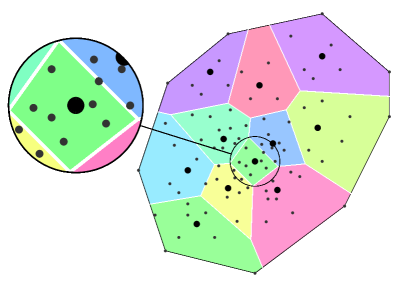
Given a sample set 𝒲Ksubscript𝒲𝐾\mathcal{W}_{K}, x0𝒮subscript𝑥0𝒮x_{0}\in\mathcal{S}, and U𝑈U, we define 𝒳Kx0,U:=X(x0,U,𝒲K)assignsuperscriptsubscript𝒳𝐾subscript𝑥0𝑈𝑋subscript𝑥0𝑈subscript𝒲𝐾\mathcal{X}_{K}^{x_{0},U}:=X(x_{0},U,\mathcal{W}_{K}) as the set of sampled state trajectories. We desire that the elements 𝒳Kx0,Usuperscriptsubscript𝒳𝐾subscript𝑥0𝑈\mathcal{X}_{K}^{x_{0},U} remain in reach-avoid set \mathcal{R}. The set 𝒳Kx0,Usuperscriptsubscript𝒳𝐾subscript𝑥0𝑈\mathcal{X}_{K}^{x_{0},U} can be partitioned into cells, where each cell consists of some of the random state trajectories and is represented by a seed. Figure 2 shows a 222D partition with 11 seeds.

Refer to caption
Figure 2: Partitioning the state uncertainty region of Figure 1 to K^^𝐾\hat{K} cells using a Voronoi partition. Larger dots indicate the selected Voronoi seeds. Samples inside each cell are closer to their own seed than other seeds.
Lemma 3.

Let ΨK^:={ψ(1),,ψ(K^)}assignsubscriptΨ^𝐾superscript𝜓1superscript𝜓^𝐾\Psi_{\hat{K}}:=\{\psi^{(1)},\cdots,\psi^{(\hat{K})}\} be the set of optimal seeds of ΦK:=ϕ(𝒲K)assignsubscriptΦ𝐾italic-ϕsubscript𝒲𝐾\Phi_{K}:=\phi(\mathcal{W}_{K}) with ϕ(W):=GwWassignitalic-ϕ𝑊subscript𝐺𝑤𝑊\phi(W):=G_{w}W that minimizes WSSWSS\mathrm{WSS}. Then 𝒳^K^x0,U=X^(ΨK^)={X^(ψ(1)),,X^(ψ(K^))}superscriptsubscript^𝒳^𝐾subscript𝑥0𝑈^𝑋subscriptΨ^𝐾^𝑋superscript𝜓1^𝑋superscript𝜓^𝐾\hat{\mathcal{X}}_{\hat{K}}^{x_{0},U}=\hat{X}(\Psi_{\hat{K}})=\{\hat{X}(\psi^{(1)}),\cdots,\hat{X}(\psi^{(\hat{K})})\} with

X^(ψ(j))=Gxx0+GuU+ψ(j),^𝑋superscript𝜓𝑗subscript𝐺𝑥subscript𝑥0subscript𝐺𝑢𝑈superscript𝜓𝑗\hat{X}(\psi^{(j)})=G_{x}x_{0}+G_{u}U+\psi^{(j)},

represents the set of optimal seeds for sampled state trajectory set 𝒳Kx0,Usuperscriptsubscript𝒳𝐾subscript𝑥0𝑈\mathcal{X}_{K}^{x_{0},U}.

Proof: Results directly from Lemma 1. Since there is no uncertainty in Gxsubscript𝐺𝑥G_{x} and Gusubscript𝐺𝑢G_{u}, Gxx0+GuUsubscript𝐺𝑥subscript𝑥0subscript𝐺𝑢𝑈G_{x}x_{0}+G_{u}U in (2) can be interpreted as a translation term.   

According to Lemma 3, although the state trajectory is an optimization variable, it can be clustered through the prediction mapping ϕ(W)italic-ϕ𝑊\phi(W) offline, independent of the choice of x0subscript𝑥0x_{0} and U𝑈U.

Lemma 4.

Let a set of points ΦKsubscriptΦ𝐾\Phi_{K}, a set of selected seeds ΨK^subscriptΨ^𝐾\Psi_{\hat{K}}, as defined in Lemma 3, and their Voronoi partition 𝒱ΦK(ΨK^)subscript𝒱subscriptΦ𝐾subscriptΨ^𝐾\mathcal{V}_{\Phi_{K}}(\Psi_{\hat{K}}) with cells VΦK(1)(ΨK^),,VΦK(K^)(ΨK^)superscriptsubscript𝑉subscriptΦ𝐾1subscriptΨ^𝐾superscriptsubscript𝑉subscriptΦ𝐾^𝐾subscriptΨ^𝐾V_{\Phi_{K}}^{(1)}(\Psi_{\hat{K}}),\cdots,V_{\Phi_{K}}^{(\hat{K})}(\Psi_{\hat{K}}) be given. Then, for j[1,K^]𝑗subscript1^𝐾j\in\mathbb{N}_{[1,\hat{K}]}, every point ϕVΦK(j)(ΨK^)italic-ϕsuperscriptsubscript𝑉subscriptΦ𝐾𝑗subscriptΨ^𝐾\phi\in V_{\Phi_{K}}^{(j)}(\Psi_{\hat{K}}) remains in the original constraint set FXh𝐹𝑋FX\leq h if ψ(j)superscript𝜓𝑗\psi^{(j)}, the jthsuperscript𝑗𝑡j^{th} seed, remains in the buffered constraint set FX^(ψ(j))hε(j)𝐹^𝑋superscript𝜓𝑗superscript𝜀𝑗F\hat{X}(\psi^{(j)})\leq h-\varepsilon^{(j)} with

ε(j)=[ϵ1(j),,ϵL(j)],superscript𝜀𝑗superscriptsuperscriptsubscriptitalic-ϵ1𝑗superscriptsubscriptitalic-ϵ𝐿𝑗top\varepsilon^{(j)}=\left[{\epsilon_{1}^{(j)}},\cdots,{\epsilon_{L}^{(j)}}\right]^{\top}, (15)

and

ϵ(j):=maxϕVΦK(j)(ΨK^)(FϕFψ(j)),[1,L].formulae-sequenceassignsuperscriptsubscriptitalic-ϵ𝑗subscriptitalic-ϕsuperscriptsubscript𝑉subscriptΦ𝐾𝑗subscriptΨ^𝐾subscript𝐹italic-ϕsubscript𝐹superscript𝜓𝑗subscript1𝐿\epsilon_{\ell}^{(j)}:=\max_{\phi\in V_{\Phi_{K}}^{(j)}(\Psi_{\hat{K}})}\left(F_{\ell}\phi-F_{\ell}\psi^{(j)}\right),\hskip 14.22636pt\ell\in\mathbb{N}_{[1,L]}. (16)

Proof: From (16) we conclude that for all [1,L]subscript1𝐿\ell\in\mathbb{N}_{[1,L]}, j[1,K^]𝑗subscript1^𝐾j\in\mathbb{N}_{[1,\hat{K}]},

FϕFψ(j)+ϵ(j)ϕVΦK(j)(ΨK^).formulae-sequencesubscript𝐹italic-ϕsubscript𝐹superscript𝜓𝑗superscriptsubscriptitalic-ϵ𝑗for-allitalic-ϕsuperscriptsubscript𝑉subscriptΦ𝐾𝑗subscriptΨ^𝐾F_{\ell}\phi\leq F_{\ell}\psi^{(j)}+\epsilon_{\ell}^{(j)}\hskip 28.45274pt\forall\phi\in V_{\Phi_{K}}^{(j)}(\Psi_{\hat{K}}). (17)

By adding F(Gxx0+GuU)subscript𝐹subscript𝐺𝑥subscript𝑥0subscript𝐺𝑢𝑈F_{\ell}\left(G_{x}x_{0}+G_{u}U\right) to the right and left sides of (17), we have

F(Gxx0+GuU+ϕ)F(Gxx0+GuU+ψ(j))+ϵ(j).subscript𝐹subscript𝐺𝑥subscript𝑥0subscript𝐺𝑢𝑈italic-ϕsubscript𝐹subscript𝐺𝑥subscript𝑥0subscript𝐺𝑢𝑈superscript𝜓𝑗superscriptsubscriptitalic-ϵ𝑗F_{\ell}\left(G_{x}x_{0}+G_{u}U+\phi\right)\leq F_{\ell}\left(G_{x}x_{0}+G_{u}U+\psi^{(j)}\right)+\epsilon_{\ell}^{(j)}. (18)

Consequently, for all ϕVΦK(j)(ΨK^)italic-ϕsuperscriptsubscript𝑉subscriptΦ𝐾𝑗subscriptΨ^𝐾\phi\in V_{\Phi_{K}}^{(j)}(\Psi_{\hat{K}}), the following holds for any initial state and input trajectory,

FX(x0,U,ϕ)FX^(x0,U,ψ(j))+ϵ(j).subscript𝐹𝑋subscript𝑥0𝑈italic-ϕsubscript𝐹^𝑋subscript𝑥0𝑈superscript𝜓𝑗superscriptsubscriptitalic-ϵ𝑗F_{\ell}X(x_{0},U,\phi)\leq F_{\ell}\hat{X}(x_{0},U,\psi^{(j)})+\epsilon_{\ell}^{(j)}. (19)

Denoting FX(x0,U,ϕ)subscript𝐹𝑋subscript𝑥0𝑈italic-ϕF_{\ell}X(x_{0},U,\phi) and FX^(x0,U,ψ(j))subscript𝐹^𝑋subscript𝑥0𝑈superscript𝜓𝑗F_{\ell}\hat{X}(x_{0},U,\psi^{(j)}) with FX(ϕ)subscript𝐹𝑋italic-ϕF_{\ell}X(\phi) and FX^(ψ(j))subscript𝐹^𝑋superscript𝜓𝑗F_{\ell}\hat{X}(\psi^{(j)}), when FX^(ψ(j))hϵ(j)subscript𝐹^𝑋superscript𝜓𝑗subscriptsuperscriptsubscriptitalic-ϵ𝑗F_{\ell}\hat{X}(\psi^{(j)})\leq h_{\ell}-\epsilon_{\ell}^{(j)}, it is concluded from (19) that FX(ϕ)hsubscript𝐹𝑋italic-ϕsubscriptF_{\ell}X(\phi)\leq h_{\ell}, ϕVΦK(j)(ΨK^)for-allitalic-ϕsuperscriptsubscript𝑉subscriptΦ𝐾𝑗subscriptΨ^𝐾\forall\phi\in V_{\Phi_{K}}^{(j)}(\Psi_{\hat{K}}). Since (19) is valid for all [1,L]subscript1𝐿\ell\in\mathbb{N}_{[1,L]} and j[1,K^]𝑗subscript1^𝐾j\in\mathbb{N}_{[1,\hat{K}]}, the proof is completed.   

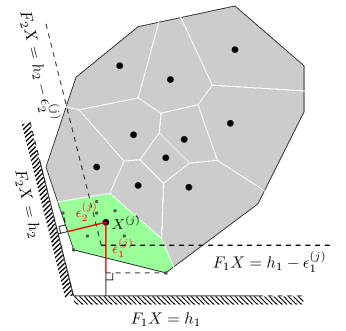
The buffering concept is illustrated in Figure 3.
Refer to caption
Figure 3: Buffering process. Cell V(j)superscript𝑉𝑗V^{(j)} is shown in green. If X(ψ(j))𝑋superscript𝜓𝑗X(\psi^{(j)}), the state trajectory corresponding to the seed of V(j)superscript𝑉𝑗V^{(j)}, remains in the buffered constraint FX(j)hϵ(j)subscript𝐹superscript𝑋𝑗subscriptsuperscriptsubscriptitalic-ϵ𝑗F_{\ell}X^{(j)}\leq h_{\ell}-\epsilon_{\ell}^{(j)}, the state trajectory of every sample in V(j)superscript𝑉𝑗V^{(j)} will satisfy the original constraint FXhsubscript𝐹𝑋subscriptF_{\ell}X\leq h_{\ell}.
Remark 2.

Computing ϵ(j)superscriptsubscriptitalic-ϵ𝑗\epsilon_{\ell}^{(j)} for =1,,L1𝐿\ell=1,\cdots,L and j[1,K^]𝑗subscript1^𝐾j\in\mathbb{N}_{[1,\hat{K}]} is a sorting problem in 111D and can be executed by worst time complexity of 𝒪(j=1K^α(j)logα(j))𝒪superscriptsubscript𝑗1^𝐾superscript𝛼𝑗superscript𝛼𝑗\mathcal{O}(\sum_{j=1}^{\hat{K}}\alpha^{(j)}\log\alpha^{(j)}).

Theorem 2.

Let ΦKsubscriptΦ𝐾\Phi_{K} be a set of K𝐾K disturbance samples mapped through the prediction mapping ϕ(W):=GwWassignitalic-ϕ𝑊subscript𝐺𝑤𝑊\phi(W):=G_{w}W and let ΨK^subscriptΨ^𝐾\Psi_{\hat{K}} be a set of selected seeds. Let α(j)=|VΦK(j)(ΨK^)|superscript𝛼𝑗superscriptsubscript𝑉subscriptΦ𝐾𝑗subscriptΨ^𝐾\alpha^{(j)}=|V_{\Phi_{K}}^{(j)}(\Psi_{\hat{K}})|, j[1,K^]𝑗subscript1^𝐾j\in\mathbb{N}_{[1,\hat{K}]}, denote the number of elements of VΦK(j)(ΨK^)superscriptsubscript𝑉subscriptΦ𝐾𝑗subscriptΨ^𝐾V_{\Phi_{K}}^{(j)}(\Psi_{\hat{K}}) and define ε(j)superscript𝜀𝑗\varepsilon^{(j)} as in Lemma 4. Problem 3 provides a lower bound for Problem 2.

Proof: According to the definition of the buffers, if seed X^(ψ(j))^𝑋superscript𝜓𝑗\hat{X}(\psi^{(j)}), j[1,K^]for-all𝑗subscript1^𝐾\forall j\in\mathbb{N}_{[1,\hat{K}]}, remains in the buffered constraint set, all α(j)superscript𝛼𝑗\alpha^{(j)} points of cell VΦK(j)(ΨK^)superscriptsubscript𝑉subscriptΦ𝐾𝑗subscriptΨ^𝐾V_{\Phi_{K}}^{(j)}(\Psi_{\hat{K}}) remain in the original constraint set. Otherwise, at most α(j)superscript𝛼𝑗\alpha^{(j)} samples belonging to cell VΦK(j)(ΨK^)superscriptsubscript𝑉subscriptΦ𝐾𝑗subscriptΨ^𝐾V_{\Phi_{K}}^{(j)}(\Psi_{\hat{K}}) may violate the original constraints. Since in Problem 3 the worst case is considered by weighting the jthsuperscript𝑗𝑡j^{th} seed with α(j)superscript𝛼𝑗\alpha^{(j)}, pK^subscriptsuperscript𝑝^𝐾p^{*}_{\hat{K}} provides a lower bound on pKsubscriptsuperscript𝑝𝐾p^{*}_{K}.   

Remark 3.

If initial state x0𝒮subscript𝑥0𝒮x_{0}\in\mathcal{S} is uncertain, the proposed method can be applied by defining ϕ(x0,W):=Gxx0+GwWassignitalic-ϕsubscript𝑥0𝑊subscript𝐺𝑥subscript𝑥0subscript𝐺𝑤𝑊\phi(x_{0},W):=G_{x}x_{0}+G_{w}W.

Obviously, having more cells results in a higher accuracy and when number of cells tends to the number of samples, pK^subscriptsuperscript𝑝^𝐾p^{*}_{\hat{K}} tends to pKsubscriptsuperscript𝑝𝐾p^{*}_{K}. However, this improved accuracy comes at a higher computational cost. We thus have to select K^^𝐾\hat{K} by trading off accuracy and computational cost.

4.2 Tightening the Voronoi-based terminal time probability estimate

Given UK^superscriptsubscript𝑈^𝐾U_{\hat{K}}^{*} obtained from Problem 3, a tighter underapproximation on pKsubscriptsuperscript𝑝𝐾p^{*}_{K} can be recalculated by simply checking the percentage of the original K𝐾K sampled trajectories that remain in reach-avoid set \mathcal{R}, after applying UK^superscriptsubscript𝑈^𝐾U_{\hat{K}}^{*} to the stochastic system. In contrast to solving a large MILP (as done in Problem 2) whose computational complexity grows exponentially with K𝐾K, this improved estimate (see (20)) is obtained by a policy evaluation that has a computational complexity of 𝒪(K)𝒪𝐾\mathcal{O}(K). The following theorem presents the probability underapproximation proposed in this paper.

Theorem 3.

Let pKsuperscriptsubscript𝑝𝐾p_{K}^{*} and pK^superscriptsubscript𝑝^𝐾p_{\hat{K}}^{*} be the optimal values of Problem 2 and Problem 3, respectively, with corresponding optimal solutions UKsuperscriptsubscript𝑈𝐾U_{K}^{*} and UK^superscriptsubscript𝑈^𝐾U_{\hat{K}}^{*}. Define p^^𝑝\hat{p} as

p^=1Ki[1,K]1(X(x0,UK^,W(i))).^𝑝1𝐾subscript𝑖subscript1𝐾subscript1𝑋subscript𝑥0subscriptsuperscript𝑈^𝐾superscript𝑊𝑖\hat{p}=\frac{1}{K}\sum_{i\in\mathbb{N}_{[1,K]}}1_{\mathcal{R}}\left(X(x_{0},U^{*}_{\hat{K}},W^{(i)})\right). (20)

Then

pK^p^pK.superscriptsubscript𝑝^𝐾^𝑝superscriptsubscript𝑝𝐾p_{\hat{K}}^{*}\leq\hat{p}\leq p_{K}^{*}.

Proof: i) Since pKsubscriptsuperscript𝑝𝐾p^{*}_{K} is the optimal terminal time probability with K𝐾K samples and p^^𝑝\hat{p} is the evaluation of an open-loop controller UK^superscriptsubscript𝑈^𝐾U_{\hat{K}}^{\ast} over these K𝐾K samples, we conclude that p^pK^𝑝superscriptsubscript𝑝𝐾\hat{p}\leq p_{K}^{*}. Equality holds if UK^=UKsuperscriptsubscript𝑈^𝐾superscriptsubscript𝑈𝐾U_{\hat{K}}^{*}=U_{K}^{*}.

ii) Let 𝒥={j[1,K^]|z^(j)=1}𝒥conditional-set𝑗subscript1^𝐾superscript^𝑧𝑗1\mathcal{J}=\{j\in\mathbb{N}_{[1,\hat{K}]}|\hat{z}^{(j)}=1\}, the subset of 𝒞superscript𝒞\mathcal{C}^{\ast} which were deemed safe by Problem 3. By definition of α(j)superscript𝛼𝑗\alpha^{(j)}, {i[1,K]:W(i)V(j)}1(X(x0,UK^,W(i)))={i[1,K]:W(i)V(j)}1subscriptconditional-set𝑖subscript1𝐾superscript𝑊𝑖superscript𝑉𝑗subscript1𝑋subscript𝑥0subscriptsuperscript𝑈^𝐾superscript𝑊𝑖subscriptconditional-set𝑖subscript1𝐾superscript𝑊𝑖superscript𝑉𝑗1\sum_{\{i\in\mathbb{N}_{[1,K]}:W^{(i)}\in V^{(j)}\}}1_{\mathcal{R}}\left(X(x_{0},U^{*}_{\hat{K}},W^{(i)})\right)=\sum_{\{i\in\mathbb{N}_{[1,K]}:W^{(i)}\in V^{(j)}\}}1 for every j𝒥𝑗𝒥j\in\mathcal{J}. In other words, since α(j)superscript𝛼𝑗\alpha^{(j)} is the set of original scenarios that fall in the jthsuperscript𝑗thj^{\mathrm{th}} cell, whenever the solution of Problem 3 deems the representative seed safe, all the scenarios within it are safe. Thus, we have p^^𝑝\hat{p} at least as big as 1Kj𝒥α(j)=p^K^1𝐾subscript𝑗𝒥superscript𝛼𝑗superscriptsubscript^𝑝^𝐾\frac{1}{K}\sum_{j\in\mathcal{J}}\alpha^{(j)}=\hat{p}_{\hat{K}}^{\ast} since there might be other cells that were not deemed safe by Problem 3 (z(j)=0)superscript𝑧𝑗0(z^{(j)}=0) but contains scenarios that might be safe (1(X(x0,UK^,W(i)))=1)subscript1𝑋subscript𝑥0subscriptsuperscript𝑈^𝐾superscript𝑊𝑖1\left(1_{\mathcal{R}}\left(X(x_{0},U^{*}_{\hat{K}},W^{(i)})\right)=1\right). Hence, p^p^K^^𝑝superscriptsubscript^𝑝^𝐾\hat{p}\geq\hat{p}_{\hat{K}}^{\ast}.   

4.3 Implementation

  Input: LTI system (1), safe set 𝒮𝒮\mathcal{S}, target set 𝒯𝒯\mathcal{T}, initial state x0subscript𝑥0x_{0}.
  
  Offline (independent of x0subscriptx0x_{0}):
  
  1. 1.

    Generate 𝒲Ksubscript𝒲𝐾\mathcal{W}_{K} by taking K𝐾K i.i.d. samples from (ηw)Nsuperscriptsubscript𝜂𝑤𝑁(\eta_{w})^{N}.

  2. 2.

    Construct ΦK=ϕ(𝒲K)subscriptΦ𝐾italic-ϕsubscript𝒲𝐾\Phi_{K}=\phi(\mathcal{W}_{K}) with ϕ(W):=GwWassignitalic-ϕ𝑊subscript𝐺𝑤𝑊\phi(W):=G_{w}W.

  3. 3.

    Select K^^𝐾\hat{K} based on the required time complexity or from the WSSWSS\mathrm{WSS} vs. K^^𝐾\hat{K} curve.

  4. 4.

    Compute ΨK^subscriptΨ^𝐾\Psi_{\hat{K}}, the optimal K^^𝐾\hat{K} seeds of ΦKsubscriptΦ𝐾\Phi_{K}, by a clustering method.

  5. 5.

    Determine 𝒱ΦK(ΨK^)subscript𝒱subscriptΦ𝐾subscriptΨ^𝐾\mathcal{V}_{\Phi_{K}}(\Psi_{\hat{K}}) with cells VΦK(1)(ΨK^),,VΦK(K^)(ΨK^)superscriptsubscript𝑉subscriptΦ𝐾1subscriptΨ^𝐾superscriptsubscript𝑉subscriptΦ𝐾^𝐾subscriptΨ^𝐾V_{\Phi_{K}}^{(1)}(\Psi_{\hat{K}}),\cdots,V_{\Phi_{K}}^{(\hat{K})}(\Psi_{\hat{K}}) from (7).

  6. 6.

    Compute importance rate vector α={α(1),,α(K^)}𝛼superscript𝛼1superscript𝛼^𝐾\alpha=\{\alpha^{(1)},\cdots,\alpha^{(\hat{K})}\} with α(j)superscript𝛼𝑗\alpha^{(j)} the number of elements of VΦK(j)(ΨK^)superscriptsubscript𝑉subscriptΦ𝐾𝑗subscriptΨ^𝐾V_{\Phi_{K}}^{(j)}(\Psi_{\hat{K}}) for j[1,K^]𝑗subscript1^𝐾j\in\mathbb{N}_{[1,\hat{K}]}.

  7. 7.

    Compute ε(j)superscript𝜀𝑗\varepsilon^{(j)} for j[1,K^]𝑗subscript1^𝐾j\in\mathbb{N}_{[1,\hat{K}]} using Lemma 4.

  
  Online (depends on x0subscriptx0x_{0}):
  
  1. 1.

    Solve Problem 3 for UK^subscriptsuperscript𝑈^𝐾U^{*}_{\hat{K}}.

  2. 2.

    Compute p^^𝑝\hat{p} from (20).

  
  Output: p^^𝑝\hat{p}.
Algorithm 1 Proposed Voronoi-based reach-avoid solution

Algorithm 1 describes the proposed Voronoi-based method to solve the open-loop terminal time problem. Given a sample set 𝒲Ksubscript𝒲𝐾\mathcal{W}_{K} with K𝐾K random samples directly drawn from (ηw)Nsuperscriptsubscript𝜂𝑤𝑁(\eta_{w})^{N}, one can construct ϕ(𝒲K)italic-ϕsubscript𝒲𝐾\phi(\mathcal{W}_{K}) and find its optimal K^^𝐾\hat{K} seeds. The k𝑘k-means method can be used to find the seeds of a Voronoi partition as explained in Section 2.4. In addition, in order to determine the number of required seeds, WSSWSS\mathrm{WSS} can be used as a measure of variability of points in a cluster. A smaller WSSWSS\mathrm{WSS} implies more compact clusters which reduces the size of defined buffers ε(1),,ε(K^)superscript𝜀1superscript𝜀^𝐾\varepsilon^{(1)},\cdots,\varepsilon^{(\hat{K})} and the average number of samples in each cell. Note that by increasing K^^𝐾\hat{K}, clusters become smaller and the precision of Problem 3 grows. However, eventually, the improvement precision is insignificant compared to the imposed computational complexity. Therefore, we compute WSS as a function of K^^𝐾\hat{K}, to explore this trade-off. We propose that the “knee” of the curve provides an efficient compromise between precision and computational complexity. It is shown experimentally in the next section that the knee of WSSWSS\mathrm{WSS} vs. K^^𝐾\hat{K} curve can be a good representative of the knee on the p^^𝑝\hat{p} vs. K^^𝐾\hat{K}. As a result, K^^𝐾\hat{K} can be computed and selected in advance.

After selecting K^^𝐾\hat{K} based on the required running time for the real-time process or based on the WSSWSS\mathrm{WSS} vs. K^^𝐾\hat{K}, one can compute the Voronoi-based partition and the number of elements in each cell, and then compute the buffers from Lemma 4. All these steps are executed offline (independent of x0subscript𝑥0x_{0}), while solving Problem 3 and probability reconstruction using (20) is done online (dependent on x0subscript𝑥0x_{0}).

5 Illustrative Example: Spacecraft Rendezvous

We consider the spacecraft rendezvous example discussed in [4]. In this example, two spacecraft are in the same elliptical orbit. One spacecraft, referred to as the deputy, must approach and dock with another spacecraft, referred to as the chief, while remaining in a line-of-sight cone, in which accurate sensing of the other vehicle is possible. The relative dynamics are described by the Clohessy-Wiltshire-Hill (CWH) equations as given in [25],

x¨3ωx2ωy˙=md1Fx,y¨+2ωx˙=md1Fy.formulae-sequence¨𝑥3𝜔𝑥2𝜔˙𝑦superscriptsubscript𝑚𝑑1subscript𝐹𝑥¨𝑦2𝜔˙𝑥superscriptsubscript𝑚𝑑1subscript𝐹𝑦\displaystyle\ddot{x}-3\omega x-2\omega\dot{y}=m_{d}^{-1}F_{x},\qquad\ddot{y}+2\omega\dot{x}=m_{d}^{-1}F_{y}. (21)

The position of the deputy is denoted by x,y𝑥𝑦x,y\in\mathbb{R} when the chief, with the mass md=300subscript𝑚𝑑300m_{d}=300 kg, is located at the origin. For the gravitational constant μ𝜇\mu and the orbital radius of the spacecraft R0subscript𝑅0R_{0}, ω=μ/R03𝜔𝜇superscriptsubscript𝑅03\omega=\sqrt{\mu/R_{0}^{3}} represents the orbital frequency. In this example, the spacecraft is in a circular orbit at an altitude of 850850850 km above the earth.

We define ζ=[x,y,x˙,y˙]4𝜁𝑥𝑦˙𝑥˙𝑦superscript4\zeta=[x,y,\dot{x},\dot{y}]\in\mathbb{R}^{4} as the system state and u=[Fx,Fy]𝒰2𝑢subscript𝐹𝑥subscript𝐹𝑦𝒰superscript2u=[F_{x},F_{y}]\in\mathcal{U}\subseteq\mathbb{R}^{2} as the system input, then discretize the dynamics (21) with a sampling time of 202020 s to obtain the discrete-time LTI system,

ζt+1=Aζt+But+wt.subscript𝜁𝑡1𝐴subscript𝜁𝑡𝐵subscript𝑢𝑡subscript𝑤𝑡\zeta_{t+1}=A\zeta_{t}+Bu_{t}+w_{t}. (22)

The additive stochastic noise, modeled by the Gaussian i.i.d. disturbance wt4subscript𝑤𝑡superscript4w_{t}\in\mathbb{R}^{4}, with 𝔼[wt]=0𝔼delimited-[]subscript𝑤𝑡0\mathbb{E}[w_{t}]=0, and 𝔼[wtwt]=104×diag(1,1,5×104,5×104)𝔼delimited-[]subscript𝑤𝑡superscriptsubscript𝑤𝑡topsuperscript104diag115superscript1045superscript104\mathbb{E}[w_{t}w_{t}^{\top}]=10^{-4}\times\mbox{diag}(1,1,5\times 10^{-4},5\times 10^{-4}), accounts for disturbances and model uncertainty.

We define the target set and the safe set as in [4],

𝒯𝒯\displaystyle\mathcal{T} ={ζ4:|ζ1|0.1,0.1ζ20,|ζ3|0.01,|ζ4|0.01},absentconditional-set𝜁superscript4formulae-sequenceformulae-sequencesubscript𝜁10.10.1subscript𝜁20formulae-sequencesubscript𝜁30.01subscript𝜁40.01\displaystyle=\left\{\zeta\in\mathbb{R}^{4}:|\zeta_{1}|\leq 0.1,-0.1\leq\zeta_{2}\leq 0,|\zeta_{3}|\leq 0.01,|\zeta_{4}|\leq 0.01\right\}, (23)
𝒮𝒮\displaystyle\mathcal{S} ={ζ4:|ζ1|ζ2,1ζ2,|ζ3|0.05,|ζ4|0.05},absentconditional-set𝜁superscript4formulae-sequencesubscript𝜁1subscript𝜁2formulae-sequence1subscript𝜁2formulae-sequencesubscript𝜁30.05subscript𝜁40.05\displaystyle=\left\{\zeta\in\mathbb{R}^{4}:|\zeta_{1}|\leq\zeta_{2},-1\leq\zeta_{2},|\zeta_{3}|\leq 0.05,|\zeta_{4}|\leq 0.05\right\}, (24)

with a horizon of N=5𝑁5N=5. We consider the initial position x=y=0.75𝑥𝑦0.75x=y=-0.75 km, the initial velocity x˙=y˙=0˙𝑥˙𝑦0\dot{x}=\dot{y}=0 km/s and 𝒰=[0.1,0.1]×[0.1,0.1]𝒰0.10.10.10.1\mathcal{U}=[-0.1,0.1]\times[-0.1,0.1]. The terminal time probability for this problem using existing approaches [10, 4] is known to be 0.860.860.86, which we assume to be the best open-loop controller-based reach-avoid probability estimate.

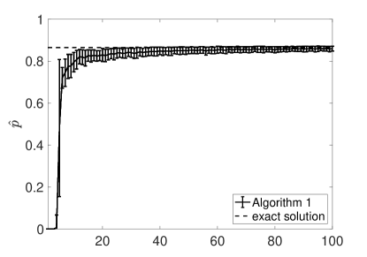
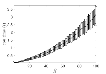
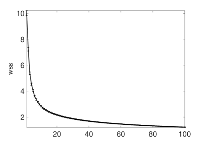
We set K=2000𝐾2000K=2000 as the number of original samples to estimate the terminal time probability, with guarantees afforded by Theorem 1, and run 100 random experiments in which in each experiment 𝒲Nsubscript𝒲𝑁\mathcal{W}_{N} is generated randomly. Simulations are carried out using CVX [26] on a 2.82.82.8 GHz processor Intel Core i555 with 161616 GB RAM. Figure 4a shows the WSSWSS\mathrm{WSS} curve (mean value and standard deviation of the results of the 100 experiments) with up to 100100100 cells. Figure 4b shows the terminal time probability approximation provided by Algorithm 1. As proposed, the “knee” of Figure 4a coincides the “knee” of Figure 4b; improvements in the accuracy of Algorithm 1 are insignificant beyond K^=20^𝐾20\hat{K}=20. In practice, K^^𝐾\hat{K} can be selected from one single experiment in which WSS𝑊𝑆𝑆WSS is calculated for a random disturbance set 𝒲Ksubscript𝒲𝐾\mathcal{W}_{K} for up to 100 (maximum allowable) cells. The computation of WSSWSS\mathrm{WSS} curve shown in Figure 4a, for one experiment using k𝑘k-means method, took only about 2.682.682.68 s, hence is reasonable for offline computation to select K^^𝐾\hat{K}. The reported time includes the computation time for solving 100100100 k𝑘k-means with 111 to 100100100 cells. This time, which is associated with offline step, can be further reduced by changing the step size of K^^𝐾\hat{K} variation (horizontal axis) or calculating WSSWSS\mathrm{WSS} for arbitrary K^^𝐾\hat{K}s (e.g. finer steps at the beginning and coarser steps at the end). The run time for the online component of Algorithm 1 is shown in Figure 4c. Since Problem 3 is a mixed-integer linear program, the time complexity exponentially increases exponentially with the number of cells [18, Rem. 1].

(a) Refer to caption
(b) Refer to caption

(c) Refer to caption

Figure 4: Mean and standard deviation of (a) within-cluster sum of squares (used to select K^^𝐾\hat{K}, offline) (b) terminal time probability (c) online run time with increasing number of cells K^^𝐾\hat{K}, obtained from 100100100 experiments with 200020002000 original scenarios.

We see in Figure 4b, that partitions with 202020 to 404040 cells provide a reasonable estimate of the terminal time probability, without significant loss of precision. The computed terminal time probability and the mean value of the online run time for K^=20^𝐾20\hat{K}=20, 404040 and 100100100 are reported in Table 1. As desired, Algorithm 1 provides a flexible trade-off between the accuracy and computation time by selecting a suitable partition, and can be significantly faster than the existing Fourier transform approach [10] and particle filter [4, 13] (which fails to deal with large K𝐾Ks due to the exponential complexity of MILP problem).

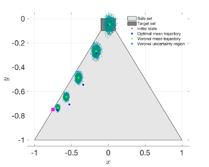
Figure 5 shows the position trajectory, associated with ζ1subscript𝜁1\zeta_{1} and ζ2subscript𝜁2\zeta_{2}, obtained by the Fourier method [10] (blue dots) and the proposed Voronoi partition-based method (green stars) with 404040 cells. Green regions show the uncertainty regions of Voronoi method at different time instants obtained by 2000 original scenarios.

Method Terminal reach-avoid probability Online run time (s)
Algorithm 1
K=2000,K^=20formulae-sequence𝐾2000^𝐾20K=2000,\hat{K}=20 0.83 0.2
K=2000,K^=40formulae-sequence𝐾2000^𝐾40K=2000,\hat{K}=40 0.8492 0.6
K=2000,K^=100formulae-sequence𝐾2000^𝐾100K=2000,\hat{K}=100 0.8604 2.7
Particle filter [4, 13] (Problem 2), K=2000𝐾2000K=2000 - -
Fourier transform [10] 0.862 66
Table 1: Terminal reach-avoid probability estimate and computation time of existing methods and Algorithm 1
Refer to caption
Figure 5: Position trajectory for Fourier algorithm given in [10] and the proposed Voronoi partition-based method with 40 cells.

6 Conclusion

In this paper we presented a novel partition-based method for under-approximating the terminal time probability through sample reduction. By using Hoeffding’s inequality, we provided a bound on the required number of scenarios to achieve a desired probabilistic bound on the approximation error. Furthermore, we proposed a method which clusters the taken scenarios in few cells, each cell represented by a seed, where the number of cells is selected by the user in a systematic manner using the trend of a given curve or based on the desired running time. The proposed method scales easily with dimension since the clustering computational complexity increases linearly with the dimension of data. In addition, the simulation results confirm that the proposed method significantly decrease the running time, and therefore, it can be easily applied to real-time systems.

References

  • [1] S. Summers and J. Lygeros, “Verification of discrete time stochastic hybrid systems: A stochastic reach-avoid decision problem,” Automatica, vol. 46, no. 12, pp. 1951–1961, 2010.
  • [2] B. HomChaudhuri, A. P. Vinod, and M. Oishi, “Computation of forward stochastic reach sets: Application to stochastic, dynamic obstacle avoidance,” in American Control Conf., Seattle, WA, 2017.
  • [3] N. Malone, K. Lesser, M. Oishi, and L. Tapia, “Stochastic reachability based motion planning for multiple moving obstacle avoidance,” in Proc. Hybrid Syst.: Comput. and Ctrl., 2014, pp. 51–60.
  • [4] K. Lesser, M. Oishi, and R. S. Erwin, “Stochastic reachability for control of spacecraft relative motion,” in Proc. IEEE Conf. Dec. & Ctrl.   IEEE, 2013, pp. 4705–4712.
  • [5] J. Gleason, A. Vinod, and M. Oishi, “Underapproximation of reach-avoid sets for discrete-time stochastic systems via Lagrangian methods,” in IEEE Conf. Dec. Ctrl., 2017. [Online]. Available: https://arxiv.org/abs/1704.03555.
  • [6] A. Abate, M. Prandini, J. Lygeros, and S. Sastry, “Probabilistic reachability and safety for controlled discrete time stochastic hybrid systems,” Automatica, vol. 44, no. 11, pp. 2724–2734, 2008.
  • [7] A. Abate, S. Amin, M. Prandini, J. Lygeros, and S. Sastry, “Computational approaches to reachability analysis of stochastic hybrid systems,” in Proc. Hybrid Syst.: Comput. and Ctrl., 2007, pp. 4–17.
  • [8] N. Kariotoglou, K. Margellos, and J. Lygeros, “On the computational complexity and generalization properties of multi-stage and stage-wise coupled scenario programs,” Syst. and Ctrl. Lett., vol. 94, pp. 63–69, 2016.
  • [9] G. Manganini, M. Pirotta, M. Restelli, L. Piroddi, and M. Prandini, “Policy search for the optimal control of Markov Decision Processes: A novel particle-based iterative scheme,” IEEE Trans. Cybern., pp. 1–13, 2015.
  • [10] A. Vinod and M. Oishi, “Scalable Underapproximation for the Stochastic Reach-Avoid Problem for High-Dimensional LTI Systems Using Fourier Transforms,” IEEE Ctrl. Syst. Letters., vol. 1, no. 2, pp. 316–321, 2017.
  • [11] ——, “Scalable underapproximative verification of stochastic LTI systems using convexity and compactness,” in Proc. Hybrid Syst.: Comput. and Ctrl., 2018, pp. 1–10.
  • [12] D. Drzajic, N. Kariotoglou, M. Kamgarpour, and J. Lygeros, “A semidefinite programming approach to control synthesis for stochastic reach-avoid problems,” in Int’l Workshop on Applied Verification for Continuous and Hybrid Syst., 2016, pp. 134–143.
  • [13] L. Blackmore, M. Ono, A. Bektassov, and B. C. Williams, “A probabilistic particle-control approximation of chance-constrained stochastic predictive control,” IEEE Trans. Robot., vol. 26, no. 3, pp. 502–517, 2010.
  • [14] H. Sartipizadeh and T. L. Vincent, “A new robust mpc using an approximate convex hull,” Automatica, 2018.
  • [15] H. Sartipizadeh and B. Açıkmeşe, “Approximate convex hull based sample truncation for scenario approach to chance constrained trajectory optimization,” in Proc. American Ctrl. Conf., 2018, pp. 4700–4705.
  • [16] G. C. Calafiore and L. Fagiano, “Stochastic model predictive control of LPV systems via scenario optimization,” Automatica, vol. 49, no. 6, pp. 1861–1866, 2013.
  • [17] G. C. Calafiore and M. C. Campi, “The scenario approach to robust control design,” IEEE Trans. Autom. Ctrl., vol. 51, no. 5, pp. 742–753, May 2006.
  • [18] A. Bemporad and M. Morari, “Control of systems integrating logic, dynamics, and constraints,” Automatica, vol. 35, no. 3, pp. 407–427, 1999.
  • [19] S. Boyd and L. Vandenberghe, Convex optimization.   Cambridge Univ. Press, 2004.
  • [20] J. A. Hartigan, Clustering algorithms.   Wiley, 1975.
  • [21] D. Aloise, A. Deshpande, P. Hansen, and P. Popat, “NP-hardness of euclidean sum-of-squares clustering,” Machine Learning, vol. 75, no. 2, pp. 245–248, May 2009. [Online]. Available: https://doi.org/10.1007/s10994-009-5103-0
  • [22] J. A. Hartigan and M. A. Wong, “Algorithm as 136: A k-means clustering algorithm,” J. Royal Statistical Society. Series C (Applied Statistics), vol. 28, no. 1, pp. 100–108, 1979.
  • [23] W. Hoeffding, “Probability Inequalities for Sums of Bounded Random Variables,” J. Amer. Statistical Asso., vol. 58, no. 301, pp. 13–30, 1963.
  • [24] M. Prandini, J. Hu, J. Lygeros, and S. Sastry, “A probabilistic approach to aircraft conflict detection,” IEEE Trans. Intelligent Transportation Syst., vol. 1, no. 4, pp. 199–220, 2000.
  • [25] W. E. Weisel, Spaceflight dynamics.   New York, McGraw-Hill Book Co, 1989, vol. 2.
  • [26] M. Grant and S. Boyd, “CVX: Matlab software for disciplined convex programming, version 2.1,” http://cvxr.com/cvx, Mar. 2014.