An optical transmission spectrum of the ultra-hot Jupiter WASP-33b

There has been increasing progress toward detailed characterization of exoplanetary atmospheres, in both observations and theoretical methods. Improvements in observational facilities and data reduction and analysis techniques are enabling increasingly higher quality spectra, especially from ground-based facilities. The high data quality also necessitates concomitant improvements in models required to interpret such data. In particular, the detection of trace species such as metal oxides has been challenging. Extremely irradiated exoplanets ($\sim$3000 K) are expected to show oxides with strong absorption signals in the optical. However, there are only a few hot Jupiters where such signatures have been reported. Here we aim to characterize the atmosphere of the ultra-hot Jupiter WASP-33 b using two primary transits taken 18 orbits apart. Our atmospheric retrieval, performed on the combined data sets, provides initial constraints on the atmospheric composition of WASP-33 b. We report a possible indication of aluminum oxide (AlO) at 3.3-$\sigma$ significance. The data were obtained with the long slit OSIRIS spectrograph mounted at the 10-meter Gran Telescopio Canarias. We cleaned the brightness variations from the light curves produced by stellar pulsations, and we determined the wavelength-dependent variability of the planetary radius caused by the atmospheric absorption of stellar light. A simultaneous fit to the two transit light curves allowed us to refine the transit parameters, and the common wavelength coverage between the two transits served to contrast our results. Future observations with HST as well as other large ground-based facilities will be able to further constrain the atmospheric chemical composition of the planet.

1 Introduction

Transiting exoplanets offer a unique opportunity to determine the physical and chemical properties of their atmospheres. In particular, the transmission spectra observed when the planet transits in front of its host star can reveal the composition and extent of the atmosphere at the day-night terminator region of the planet. Here, the extinction of the stellar photons travelling through the planetary atmosphere along the line of sight is imprinted on the observed stellar spectrum during the transit. Time-domain differential spectroscopy, between in and out of transit, reveals the absorption spectrum of the planetary atmosphere, also known as a ”transmission” spectrum. This technique and its variants have been used to detect several atomic and molecular species in exoplanetary atmospheres; for example sodium Charbonneau et al. (2002); Snellen et al. (2008); Redfield et al. (2008), H₂O and CO Snellen et al. (2010); Deming et al. (2013); Kreidberg et al. (2014b), and clouds and hazes Bean et al. (2010); Pont et al. (2013); Kreidberg et al. (2014a).

To characterize the chemical compositions of exoplanetary atmospheres two approaches of transit spectroscopy have been successfully used. High resolution transmission spectroscopy is ideally suited to resolve individual absorption lines of the chemical species in the atmosphere, in other words, via the imprint of the planetary lines on the stellar spectrum (e.g., Snellen et al., 2008; Wyttenbach et al., 2015; Khalafinejad et al., 2017). This technique first led to the detection of sodium in the atmosphere of HD 209458b from high-precision spectro-photometric observations (Charbonneau et al., 2002). At resolutions of R$\sim$100 000, the absorption line cores of individual chemical species such as sodium can be spectroscopically resolved, as well as the orbital motion, the diurnal rotation, and in some extreme cases exo-atmospheric wind speeds (Snellen et al., 2010; Louden & Wheatley, 2015). On the other hand, the use of low resolution spectra and broadband photometry allows investigations of broad spectral features over a wide wavelength range, such as the presence of clouds, hazes or Rayleigh scattering, along with strong atomic and molecular absorbers (e.g., Sing et al., 2016; Mallonn & Strassmeier, 2016; von Essen et al., 2017; Mallonn & Wakeford, 2017; Nikolov et al., 2018).

In tandem with observational advancements, there have also been key developments in atmospheric modeling of exoplanets. Several studies predict key atomic and molecular species to be present in exoplanetary atmospheres depending on the macroscopic conditions such the equilibrium temperature, gravity, and metallicity (see e.g., Seager & Sasselov, 2000; Hubbard et al., 2001; Fortney et al., 2010; Madhusudhan et al., 2016a). Early theoretical modeling suggested Hot Jupiters with equilibrium temperatures above 2500 K to be similar to M dwarfs containing gaseous oxides such as TiO and VO in cloud-free atmospheres (Hubeny et al., 2003; Fortney et al., 2008). The strong opacity of TiO/VO at optical wavelengths could result in thermal inversions, that is, rising temperatures with higher altitudes (Burrows et al., 2008). The first observational evidence for such inversion layers were published for a much cooler Hot Jupiter (Knutson et al., 2008). However, this and several other measurements were revised subsequently (see e.g., Diamond-Lowe et al., 2014; Hansen et al., 2014; Evans et al., 2015). In parallel, several mechanisms were investigated explaining why gaseous TiO might not play a role in the physics of the high altitude layers, including the gravitational settling to colder atmospheric layers were the molecules condense out as well as the carbon to oxygen ratio (Spiegel et al., 2009; Parmentier et al., 2013; Madhusudhan, 2012).

Recently, promising indications for the presence of TiO have been published for two of the hottest gas giants known. In the terminator region of the $T_{\mathrm{eq}}=2400$ K WASP-121b, Evans et al. (2016) found hints of additional opacity at optical wavelengths, indicative of TiO. Shortly thereafter, Evans et al. (2017) found stronger evidence for TiO and a thermal inversion in the day-side of the same planet. Transmission spectroscopy of WASP-19b ($T_{\mathrm{eq}}=2100$ K) resolved optical absorption bands from TiO (Sedaghati et al., 2017). However, measurements for the similarly hot gas giants WASP-12b ($T_{\mathrm{eq}}=2600$ K) showed no signs of TiO absorption at the terminator, making it more likely that these elements have been removed from these parts of the planetary atmosphere (Sing et al., 2013). Another difference between these three very hot gas giants is the level to which the transmission spectra are dominated by clouds and hazes. While it is substantial enough for WASP-12b to cause a featureless optical spectrum (Sing et al., 2013), the atmospheres of WASP-19b and WASP-121b seem to be less affected, showing absorption features. The formation of condensate clouds in ultra-hot Jupiter atmospheres was investigated by Wakeford et al. (2017).

The TiO signals in WASP-19b and WASP-121b have so far been the strongest evidence for the presence of the debated gaseous TiO, indicating a dependence of temperature. One of the hottest planets after KELT-9b is WASP-33 b with measured brightness temperature at its dayside of T_B = 3398 $\pm$ 302 K (von Essen et al., 2015). Very recently, Nugroho et al. (2017) found significant signal of TiO in its dayside including indications for a thermal inversion. The existence of this stratosphere in its dayside was also suggested by Haynes et al. (2015). An investigation of the phase curve of WASP-33 b by Zhang et al. (2018) described the planets heat recirculation as similar to cooler Hot Jupiters.

In this work we present the search for oxides and clouds and hazes at the terminator region of the atmosphere of WASP-33 b (Collier Cameron et al., 2010) by transmission spectroscopy in the optical. We exploit two transit observations taken 18 orbits apart with the 10 meter Gran Telescopio Canarias. The exoplanet orbits an A-type star every $\sim$1.22 days, making it one of the strongest irradiated planets known till date (Smith et al., 2011; von Essen et al., 2015). The host is a $\delta$ Scuti star, with pulsation amplitudes in the milli-magnitude regime and frequencies on the order of a few hours (Herrero et al., 2011; von Essen et al., 2014). Lehmann et al. (2015) carried out a spectroscopic follow-up of the host star, characterizing the mass of the planet to be around 2.1 M_J. WASP-33 b shows an unusually large radius ($\sim$1.6 R_J), making it inflated (Collier Cameron et al., 2010) and ideal for transmission spectroscopy studies. Along a 2.5-year photometric follow up we have characterized the pulsation spectrum of the host star (von Essen et al., 2014). From this analysis we found eight statistically significant pulsation frequencies, most of them well contained within a typical ground-based observation. Their proper representation is fundamental to correctly determine the transmission spectrum of WASP-33 b. In this work, Section 2 presents the observations and the data reduction, Section 3 shows a detailed description of the model parameters and fitting procedures, Section 4 shows our results on the transmission spectrum of WASP-33and constraints on its atmospheric properties, while Section 5 contains our final remarks.

2 Observations and data reduction

2.1 Instrumental setup

On the nights of August 7th (henceforth observing run 1, OR1) and August 30th (observing run 2, OR2), 2014, we simultaneously observed WASP-33 (V = 8.14) and the star BD+36 488 (V = 9.37) during primary transit. For our observations we used the longslit spectroscopic mode of OSIRIS, mounted at the 10-meter Gran Telescopio Canarias, Spain. The observations were carried out in its standard observing mode (binning 2$\times$2). To avoid saturation of the target we observed with the telescope slightly defocused. To minimize flux losses (e.g., Sing et al., 2012) the slit was opened to 10 arcsec.

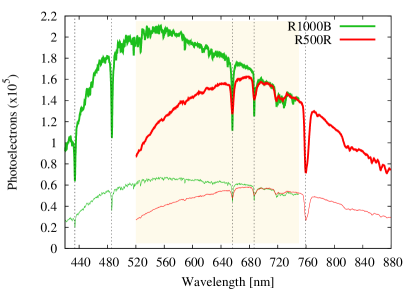
During OR1 we observed WASP-33 using the R1000B grism (spectral resolution, R = 1018), which allows for a wavelength coverage between 363 and 750 nm. We collected 587 spectra along a total of 4.24 hours, starting at 1:31 UT and finishing at 5:45 UT. Our observations cover the primary transit fully, plus about one our before and one hour after transit, respectively. The exposure time was set to one second. Due to readout time the final cadence of the data was 25 seconds. For OR1 we integrated fluxes between 420 and 750 nm, avoiding the wavelengths where the signal was too low. During OR2 we observed WASP-33 for 4.4 hours using the R500R grism (R = 587), covering the wavelengths between 480 and 1000 nm. The exposure time was set to 0.4 seconds. Using a faster readout mode, the final cadence was 19 seconds. The observations started at 0:11 UT and ended at 4:35 UT, which corresponds to full transit coverage plus an hour before and after transit, respectively. We considered fluxes between 520 and 880 nm, and neglected the wavelength region around telluric oxygen (760 $\pm$ 10 nm). The considered wavelength coverage for each one of the grisms, along with the instrumental fluxes of WASP-33 and BD+36 488, can be seen in Figure 1.

Figure 1: Extracted spectra in photoelectrons for WASP-33 (continuous thick lines) and BD+36 488 (continuous thin lines) for the R1000B and R500R grisms (green and red colors, respectively). Vertical dashed black lines indicate the atmospheric and stellar lines used to align the spectra. The yellow shaded region highlights the wavelength coverage of the data sets used to construct the white light curves (see Section 3.1).

2.2 Spectral extraction and determination of environmental quantities

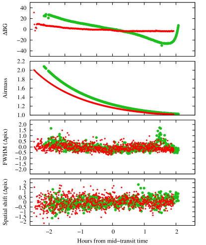
Before extracting the spectra, we began our analysis by computing the changes in airmass, seeing, centroid positions and background analyzing each stellar spectra. Airmass values were extracted from the header of the images. We fitted a Gaussian function to several cuts along the two-dimensional spectra. The fitting parameters are the means, $\mu$ and standard deviations, $\sigma$. The one-on-one differences of the means between the frame with the lowest airmass (i.e., the reference frame) and all the remaining frames were averaged and used to estimate the spatial shifts. The changes of full-width at half-maximum (FWHM) were determined from FWHM = 2$\sqrt{2ln(2)}<\sigma>$, where $<\sigma>$ is the average of the standard deviations. Background values were computed averaging the number of counts in predefined regions left and right from WASP-33’s spectra, along all wavelengths. Figure 2 shows these quantities as a function of time. In the figure, time is given in hours from mid-transit time. Both nights are photometrically stable, and the spatial shifts are well contained within two binned pixels. Due to the observed spatial stability, we did not flat-field the spectra. This would only add an unnecessary source of noise. To test this, we produced light curves with and without flatfielding the spectra, finding no significant difference with respect to the photometric precision of the derived spectro-photometric light curves. The light curves produced from flatfielded data showed only slightly larger photometric scatter.

To avoid saturation of the target, the telescope was scarcely defocused. In consequence, we can not report averaged seeing values from our data. Typical seeing on Roque de los Muchachos observatory is about or below 1 arcsec. During OR1 the FWHM was $\sim$2.7 arcsec, while for OR2 it was around 2.8 arcsec, thus we do not expect significant flux loses in the 10^′′ slit. We carried out the wavelength calibration in the usual way, using the identify IRAF task. The RMS of the pixel-to-wavelength conversion was, in both runs, lower than 0.05 arccec/pixel, well contained within the spectral resolution. Since the exposure time was low in both observing nights, we did not carry out cosmic ray removal.

Before extracting stellar fluxes, we carried out the background subtraction with IRAF’s task apall, fitting the sky spectrum with a constant offset along predefined background regions at least 10 FWHM away from the WASP-33 spectra in the spatial direction spectra. To test the impact of the aperture size into the accuracy of the spectro-photometric light curves, we extracted the one-dimensional spectra using IRAF’s apall task with apertures of between 1 and 15 arcseconds in steps of 1 arcsecond. For this exercise, photometric light curves were produced integrating fluxes between 520 and 750 nm for both OR1 and OR2. We then computed the standard deviation of each light curve taking into account only the off-transit data points, and chose the final apertures that minimized this standard deviation. As an independent test we also fitted a high order time-dependent polynomial to the data, that accounted for the transit shape and the pulsations of the host star. We then computed the standard deviation of the residuals, obtained subtracting this best-fit nonphysical polynomial to the photometric data sets. In both cases, and for both transits, the aperture minimizing the previously mentioned standard deviations was found to be 6 arcseconds. It is worth to mention that large apertures minimizing the standard deviation of the data have been observed before in spectrophotometric transit observations with OSIRIS (Mallonn et al., 2015; Mackebrandt et al., 2017; Chen et al., 2017).

Figure 2: From top to bottom, time-dependent changes of background counts (BG), airmass, FWHM, and spatial shifts. Both data sets have been shifted to their respective mid-transit times, and are shown in hours. Large green circles correspond to the R1000B (OR1) data, while small red diamonds correspond to R500R (OR2).

Throughout this work, time stamps are converted from the Julian Dates extracted from the header of the images to Barycentric Julian Dates, BJD_TDB. To carry out this conversion, we used the tools made available by Eastman et al. (2010).

3 White light curve: Data preparation and main analysis

3.1 Construction of light curves and computation of spectro-photometric errors

The two white light curves (OR1 and OR2) were constructed integrating the fluxes of both target and reference stars in the wavelengths between 520 and 750 nm (see shaded area on Figure 1). Limiting the wavelength region was intended to minimize any impact related to the wavelength-dependency of the pulsation amplitudes (e.g., Breger et al., 2005), and limb darkening differences between the two data sets. Although some flux was lost, this allowed us to carry out a coherent, simultaneous fit of both transit and pulsations. The Fraunhofer and stellar lines indicated with dashed vertical lines in Figure 1 were used to check that the spectra were aligned within each night, and among OR1 and OR2.

We computed the spectro-photometric errors using the formalism provided by IRAF, as described in detail in Sect. 3.2 of von Essen et al. (2017). In brief, uncertainties are computed using the integrated fluxes within a given wavelength range and chosen aperture, the respective area, the standard deviation of the sky region within the same wavelength range, the number of sky pixels, and the gain of the detector. Since errors determined in this way are known to be slightly underestimated (Gopal-Krishna et al., 1995), we scaled them up to meet the standard deviation of the off-transit data points. In this way, the spectro-photometric errors reflect not only the natural scatter of the data, but also the expected increase of noise with increasing airmass.

Huitson et al. (2017) reported the impact of wavelength-dependent ”stretches” in spectroscopic data over chromatic light curves, all wrapped up in the context of transmission spectroscopy studies. The stretches occur when a given pixel does not sample the same wavelength in each exposure, mostly due to be mechanical or atmospheric causes. The authors computed these stretches from cross-correlating their GEMINI/GMOS spectra during transit solely around the Na and H$\alpha$ lines. Their derived variability has an amplitude of about one pixel (their Figure 2). As expected, the authors found this effect to be more prominent for narrower wavelength bins than the ones they were using ($\sim$10 nm). Even though they failed at reproducing this variability by a physically-motivated model, they identify it to be connected to the instrument response function. For response functions steepening toward bluer wavelengths, the introduced flux changes should be more prominent and, thus, increase the error on the derived transmission spectrum.

To characterize this effect over our GTC/OSIRIS data and the potential impact on our results, we carried out the same procedure as in Huitson et al. (2017). Our derived stretches perfectly mimic the variability observed with FWHM, and the latter is found unimportant in the data detrending process by the BIC (see Section 3.4). Following the behaviour observed in Figure 2 (red points), the stretches for R500R have no systematic noise. Only white noise around $\pm$1 Å (equivalently, $\pm$0.2 pixels). In the case of R1000B (green points in Figure 2) the stretches have a systematic trend in agreement with the FWHM variability. However, the amplitude is smaller as the spectra are of better quality and, thus, the cross-correlation naturally improves. In this case, most of the points lie around $\pm$0.3 Å (equivalently, $\pm$ 0.1 pixels). All in all, our integration bands are double the size (20 vs. 10 nm), which would dilute this effect by construction. Furthermore, our derived stretches are on average an order of magnitude smaller. We did not consider for our analysis of the transmission spectrum the edges of the spectra, and in consequence we do not account in our analysis fluxes showing the largest pixel-to-pixel variability. Thus, we believe this effect is negligible. To avoid carrying out unnecessary changes to an already complicated data set, in this work we do not correct for the observed stretches.

From the derived light curves we first noticed a large scatter, growing with increasing airmass. Due to short exposure times and the large collecting area of the GTC, our photometric precision is strongly limited by scintillation (Young, 1993; Kjeldsen & Frandsen, 1992). However, owing to the large flux of both stars the choice of the integration band does not significantly affect the noise of the wavelength-binned light curves. Therefore, the impact of choosing a narrower integration band to construct the white light curves did not significantly diminished their overall quality. To fit the transit light curves we take into account a model with three main components: a transit, a detrending, and a pulsation model.

3.2 The transit model

As primary transit model we use Mandel & Agol (2002)’s occultquad routine. The parameters that we can infer are the semi-major axis in stellar radii, $\mathrm{a/R_{s}}$, the orbital inclination, i, the orbital period, Per, the mid-transit time, T₀, the planet-to-star radius ratio, $\mathrm{R_{P}/R_{S}}$, and the limb darkening coefficients, $\mathrm{u_{1}}$ and $\mathrm{u_{2}}$, from a quadratic limb-darkening law.

Throughout this work, limb darkening coefficients are computed as described in von Essen et al. (2017) for specific wavelength regions, for each transit, and for stellar parameters closely matching the ones of WASP-33. In order to properly compute the limb-darkening coefficients, the efficiency of both CCD and grisms -along with their wavelength dependency- have to be taken into consideration. Since the optical setup differs between one transit and the other, simply because two different grisms were used, we computed a set of linear and quadratic limb darkening coefficients per observing run. For the white light curve the derived values for OR1 are u₁ = 0.333(1) and u₂ = 0.245(6). For OR2, the limb darkening coefficients are u₁ = 0.322(9) and u₂ = 0.243(1). The similarity between the two sets of LDs does not come as a surprise. While the star and the integration wavelength region are exactly the same, the responses of the two grisms are similar. For the derived values, parenthesis indicate the precision in the fit of the stellar intensities as a function of distance between the stellar limb and center. As pointed out in von Essen et al. (2017) and as observed by Kervella et al. (2017), the precision of the limb-darkening coefficients only reflects a goodness of fit between models and a second order polynomial, and not the true accuracy at which we know any limb-darkening coefficients. The photometric precision of our data does not allow to detect differences in limb darkening in the third decimal. Therefore, for both white light curves we used as linear and quadratic limb-darkening values their average. This means that we fit only one transit model to the two data sets, simplifying the number of parameters. Further considerations in the wavelength-dependent light curves will be given in future sections. For WASP-33A, we considered stellar atmospheric models provided by PHOENIX (Hauschildt & Baron, 1999; Witte et al., 2009) for a surface gravity of 4.5, an effective temperature of 7400 K, and a metallicity of 0, closely matching WASP-33’s values reported by Collier Cameron et al. (2010) ($\log(g)=4.3\pm 0.2$, $T_{eff}$ = 7430 $\pm$ 100 K, and [Fe/H] = 0.1 $\pm$ 0.2, respectively).

Along this work, the limb darkening coefficients are considered as fixed, and are computed in the same way described here per integration band width. We fitted all the transit parameters, with the exception of the orbital period (von Essen et al., 2014), since its known to a high degree of accuracy. For the transit parameters we considered Gaussian priors using as starting values the ones derived in von Essen et al. (2014) (where the pulsations were accounted for) and as width for their Gaussian priors five times their errors.

3.3 Pulsation model

As done in von Essen et al. (2015), to represent the stellar pulsations our model comprises the sum of eight sinusoidal functions. Here, the model parameters are the pulsation frequencies, amplitudes and phases. To constrain the parameter space we used our prior knowledge about the pulsation spectrum of the star, along with its behaviour in time. For instance, in von Essen et al. (2014) (see Section 3.5) we detected a time-dependent change of the phases of the pulsations. In order to characterize their shifts, we divided the data in monthly groups and computed the shifts there. The closest two groups were taken one month apart, which is approximately the time between OR1 and OR2. Within this time lapse, some of the pulsations showed differences in phases smaller than 0.2$\times$2$\pi$ (pulsations 1, 4, and 6), while the others showed a phase shift with an amplitude up to 0.4$\times$2$\pi$. To both minimize the number of fitting parameters and take the phase shifts into consideration, our pulsation model comprises eight phases that are fitted simultaneously to the two transits, plus eight phase shifts. We note, however, that both phases and phase shifts can be degenerate. Thus, we fit them to the data using Gaussian priors. Each shift has a Gaussian distribution around zero, with standard deviations equal to the previously mentioned phase shift amplitudes. Each phase has a Gaussian distribution around our best initial guesses, with a standard deviation equal to 0.2. This value is completely arbitrary. Since OR1 and OR2 are two years apart from the data analyzed in von Essen et al. (2014) and we don’t know how the phases continuously evolve in time, we don’t know their current values. Our initial guesses were thus computed evaluating the pulsation model in different phase values, particularly dividing each phase space in a grid ranging from 0 to 1 and a step of 0.05. Our initial estimates for the phases are the ones that minimize the standard deviation of the light curves once each pulsation model is subtracted.

As the frequency resolution is 1/$\Delta$T (Kurtz, 1983), 2$\times$4 hours of data are not sufficient to determine the pulsations frequencies. Therefore, during our fitting procedure we used the frequencies determined in von Essen et al. (2014) as fixed values. Furthermore, it is known that $\delta$ Scuti stars have pulsation amplitudes that are also wavelength dependent (Breger, 1979; Breger et al., 2005). The observations performed in von Essen et al. (2014) were taken mostly in the visible ($\sim$550 $\pm$ 70 nm) not matching with the wavelength coverage of the white light curves. Since the overall amplitudes of the pulsations are small and differential variability is not detectable from the photometric precision of our data, at this stage, the amplitudes are considered as fixed parameters with values equal to the ones derived in von Essen et al. (2014). However, we account for any possible offset between these and those from our observations by adding to our model parameter space a constant amplitude offset per wavelength channel equal to all the eight amplitudes, and to the two transits, separately. In other words, while the transit parameters are fitted simultaneously to the two light curves, the amplitudes in the wavelength bins that match between OR1 and OR2 are completely disconnected. However, if the wavelength range is the same for two given light-curves between OR1 and OR2, as it is the case of the white light curves, the resulting amplitude offsets should be consistent between each other. The results obtained from this approach will serve as consistency check of our methodology. All in all, the pulsation model (PM) is as follows:

$$\mathrm{PM(t)} = \mathrm{PM(t)_{OR1}+PM(t)_{OR2}}$$ (1)

$$= \sum_{i=1}^{8}(A_{i}+A_{j})\times\sin[2\pi(\nu_{i}t+\phi_{i})]+$$

$$\sum_{i=1}^{8}(A_{i}+A_{k})\times\sin[2\pi(\nu_{i}t+\phi_{i}+\Delta\phi_{k})]\,.$$

Here $\mathrm{A_{i}}$ and $\mathrm{\nu_{i}}$ correspond to the eight amplitudes and frequencies found in von Essen et al. (2014) considered as fixed, $\mathrm{\phi_{i}}$ are the eight fitted phases, and $\mathrm{A_{j}}$ and $\mathrm{A_{k}}$ are scaling factors that account for wavelength-dependent amplitude differences. The indexes j and k range between one and the number of wavelength bins of OR1 and OR2, respectively. Thus, for the white light curves j = 1 and k = 1. $\mathrm{\Delta\phi_{k}}$ accounts for the phase shifts between OR1 and OR2. The best-fit amplitudes and phases can be seen in Table 2. For both OR1 and OR2, the values of the phases are absolute, and not differential. The amplitudes of OR1 and OR2 are fully consistent within 1-$\sigma$ uncertainties, and the phase differences are within the expected ranges. The errors of the phases are purely statistical and are influenced by our choice of using Gaussian priors. Thus, they should be considered with care.

3.4 Detrending model

To account for systematic noise in our data, we tested several dependencies. Due to the deformations caused by the pulsations it is hard to visually inspect the success of our detrending strategy. Thus, to choose the amount of detrending components we made use of the minimization of the Bayesian Information Criterion, BIC = $\chi^{2}$ + k ln N. For the BIC, k is the number of model parameters and N is the number of data points. Besides the linear and quadratic time-dependent polynomials, we used a linear combination of airmass (also considered quadratically), FWHM, background counts and spatial position, combining them in several ways. The detrending function minimizing the BIC corresponds to a quadratic function of airmass plus a linear function of background counts. This coincides with the variability observed in Figure 2. The FWHM and the spatial position, not favored by the BIC, are actually the ones that vary the less along the ORs. The detrending model (DM) looks as follows:

$$\mathrm{DM(t)}=c_{0}+c_{1}\times\chi+c_{2}\times\chi^{2}+c_{3}\times bc,\,$$ (2)

where $c_{0}$, $c_{1}$, $c_{2},$ and $c_{3}$ are the detrending coefficients, $\chi$ corresponds to the airmass, and bc to the background counts. The four detrending coefficients have all uniform priors. Since stellar light suffers a wavelength-dependent absorption when crossing our atmosphere, a set of four detrending coefficients is fitted to each chromatic light curve individually.

3.5 Computation of model parameters

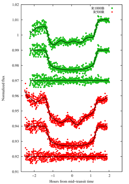
To derive the model parameters we fitted the two white light curves simultaneously using a Markov-chain Monte Carlo (MCMC) approach, all wrapped up in PyAstronomy, a collection of Python routines providing a convenient interface for fitting and sampling algorithms implemented in the PyMC (Patil et al., 2010) and SciPy (Jones et al., 2001) packages. After 1$\times$10⁶ iterations and a burn-in of the initial 2$\times$10⁵ samples, we computed the mean and standard deviation (1-$\sigma$) of the posterior distributions of the parameters and used them as best-fit values and uncertainties, respectively. The best-fit solutions, along with their errors, are displayed in Table 1. To check for convergence of the MCMC chains we divided them in three equally large subgroups and computed their respective mean and standard deviations. We considered a chain to converge if these values were consistent between each other at 1-$\sigma$ level. We finished up with a visual inspection of the chains. The transit photometry corresponding to OR1 and OR2, the best-fit model, the detrended light curves and the residual light curves can be seen in Figure 3. The transit parameters derived in this work show smaller uncertainties than bibliographic values.

Figure 3: White light curves of WASP-33 b obtained with the GTC, artificially shifted for visual inspection. Green filled circles correspond to OR1, and red filled diamonds to OR2. Each OR is presented in three sections, described from top to bottom as follows: the raw photometry along with the best-fit model in black continuous line, the transit light curve after the pulsations and detrending models are subtracted, along with the best-fit transit model in black continuous line, and the residual light curves on the bottom.

Table 1: Best-fit parameters derived from the two white light curves, compared to the values reported in von Essen et al. (2014).

Parameter	OR1/OR2	von Essen et al. (2014)
a/Rs	3.62 $\pm$ 0.02	3.68 $\pm$ 0.03
i (∘)	88.24 $\pm$ 0.28	87.90 $\pm$ 0.93
RP/Rs	0.1053 $\pm$ 0.0004	0.1046 $\pm$ 0.0006
T0 (BJDTDB)	1878.65739 $\pm$ 0.00015	507.5222 $\pm$ 0.0003
Per (days)	1.2198675 (fixed)	1.2198675 $\pm$1.1$\times$10-6
u1	0.327(8) (fixed)	(see Table 8, von Essen et al. (2014))
u2	0.244(3) (fixed)	(see Table 8, von Essen et al. (2014))

Table 2: Best-fit phases, $\phi_{i}$, and amplitudes, $\mathrm{A_{j}}$ and $\mathrm{A_{k}}$, derived from the two white light curves. Amplitudes are given in parts-per-thousand (ppt), phases in units of 2$\pi$, and the subindices follow the notation of Eq. 1.

Parameter	OR1	OR2
$\phi_{\mathrm{1}}$	0.334 $\pm$ 0.005	0.676 $\pm$ 0.005
$\phi_{\mathrm{2}}$	0.644 $\pm$ 0.005	0.334 $\pm$ 0.005
$\phi_{\mathrm{3}}$	0.867 $\pm$ 0.005	0.583 $\pm$ 0.005
$\phi_{\mathrm{4}}$	0.114 $\pm$ 0.005	0.984 $\pm$ 0.005
$\phi_{\mathrm{5}}$	0.843 $\pm$ 0.005	0.462 $\pm$ 0.005
$\phi_{\mathrm{6}}$	0.089 $\pm$ 0.005	0.116 $\pm$ 0.005
$\phi_{\mathrm{7}}$	0.323 $\pm$ 0.005	0.475 $\pm$ 0.005
$\phi_{\mathrm{8}}$	0.356 $\pm$ 0.005	0.691 $\pm$ 0.005
Aj/k	0.22 $\pm$ 0.05	0.19 $\pm$ 0.05

3.6 Treatment of correlated noise

Although our model accounts for the deformations produced by the pulsations, these are actually the ones that do not allow us to visually assess whether the detrending model is sufficient to describe our data. At this stage, we reply purely on statistical tools such as the BIC. To account for as much as possible either systematic effects not accounted for in our model, or a poor pulsation model (i.e., not enough pulsation frequencies yet discovered), we carried out the MCMC fitting process twice. After the first MCMC run that was carried out as described in the previous section, we computed residual light curves for OR1 and OR2 subtracting our best-fit models to each photometric light curve. Following the approach described in Gillon et al. (2006); Winn et al. (2008); Carter & Winn (2009), we computed the $\beta$-value from the residual light curves following their prescription, averaging $\beta$’s calculated within time bins equal to 0.8, 0.9, 1, 1.1, and 1.2 times the transit ingress/egress time. Then, we enlarged the spectro-photometric error bars by the $\beta$’s, and we re-run MCMC to re-compute the best-fit parameters. The derived values are reported in Table 1, and the $\beta$ values are $\beta_{OR1}$ = 1.05, and $\beta_{OR2}$ = 1.29.

3.7 Construction of the wavelength-binned light curves and corresponding fitting parameters

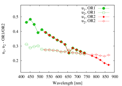
To derive the transmission spectrum of WASP-33 b from color-dependent light curves, we carried out a similar approach than the one of the white light curve regarding the computation of spectro-photometric errors, their respective scaling to meet the standard deviation, the computation of correlated noise, and the calculation of limb-darkening coefficients. To obtain the best-fit planet-to-star radius ratio as a function of spectral bin we made use of MCMC in the exact same fashion as with the white light curves. The values of planet-to-star radii ratio reported in this work are thus obtained from the second MCMC run of 1$\times$10⁶ iterations, after a burn-in phase of the first 2$\times$10⁵ samples. To compute the chromatic light curves we divided the total spectral coverage in wavelength bins with a width of $\sim$22 nm. Figure 4 shows the derived linear (full green circles) and quadratic (empty green circles) limb-darkening coefficients for OR1, along with the corresponding ones for OR2 (filled and empty red diamonds, respectively). As the figure reveals, there is an almost identical match between the limb-darkening values derived from the two observing runs in the wavelength regions where they coincide. The small differences are caused by the slightly different responses of the used grisms, R1000B and R500R.

Figure 4: Limb-darkening coefficients, u₁ and u₂, for OR1 in green circles and OR2 in red diamonds. The linear and quadratic coefficients are plotted in filled and empty points, respectively.

The strength at which absorption of stellar light takes place in our atmosphere strongly depends on wavelength and airmass. For both OR1 and OR2, airmass values at the beginning of the observations were slightly larger than 2. Therefore, our chromatic light curves have a differential deformation that can clearly be distinguished by visually inspecting the raw light curves. To account for this, we fit the four detrending coefficients to each light curve independently. We also tested a common mode correction by dividing the chromatic light curves by the white light curve residuals (see e.g., Lendl et al., 2016; Nikolov et al., 2016; Gibson et al., 2017). However, this exercise did not reduce the noise in the chromatic light curves nor did it notably change the results. Therefore, it was finally not included in the analysis procedure.

In order to properly propagate the errors on the transit parameters to the chromatic light curves, rather than fixing the transit parameters derived from the white light curves these were set free. In all cases the planet-to-star radius ratio, R_P/R_S, was fitted considering a uniform probability density function limited between 0 and 0.3, way above and below bibliographic values. The semi-major axis, inclination and mid-transit time were fitted to the chromatic light curves using Gaussian probability density functions with mean and standard deviation equal to the best-fit and error values obtained from the white light curves, respectively. These parameters do not depend on wavelength. In consequence, we treated them as equal during the MCMC fitting.

Equivalently to the transit parameters, rather than fixing the sixteen phases to the values obtained from the white light curves, these were fitted to the chromatic light curves simultaneously. Thus, rather than having (8$\times$2)$\times$n fitting phases, where n is the number of wavelength channels, we fitted only 8x2. As initial values we used the ones obtained from the white light curve analysis, along with a Gaussian probability density function with standard deviation equal to the reported 1-$\sigma$ errors. Finally, to account for wavelength-dependent variations of the pulsation amplitudes we considered the previously mentioned amplitude offset, A_j/k. We fitted one amplitude offset to each chromatic light curve, using uniform priors between -0.1 and 0.1 ppt. Pulsation amplitudes are expected to grow with stellar emission. Since WASP-33 emits most of its flux in the bluer wavelengths, it is expected for A to grow with decreasing wavelength. Figure 5 shows the best-fit values of A_j/k, along with 1-$\sigma$ uncertainties for OR1 (green filled circles) and OR2 (red filled diamonds). The figure shows two very important results. On one hand, as expected in $\delta$ Scuti stars the amplitude offset relative to the amplitudes found in von Essen et al. (2014) does decrease with increasing wavelength. On the other hand, even though the pulsation amplitudes were fitted to each transit with uniform priors individually, within 1-$\sigma$ errors they perfectly overlap in the common wavelength region.

Figure 5: Amplitude offset, A_j/k, as a function of wavelength channel. Here, j represents the wavelength channels of OR1, and k the ones of OR2. Best-fit values and 1-$\sigma$ uncertainties are plotted in green filled circles for OR1, and in red filled diamonds for OR2.

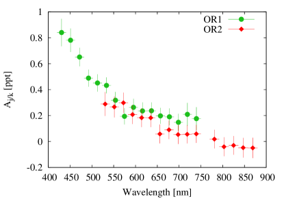
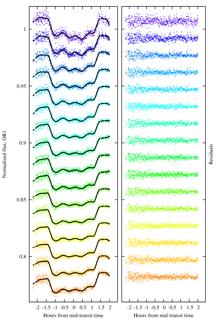
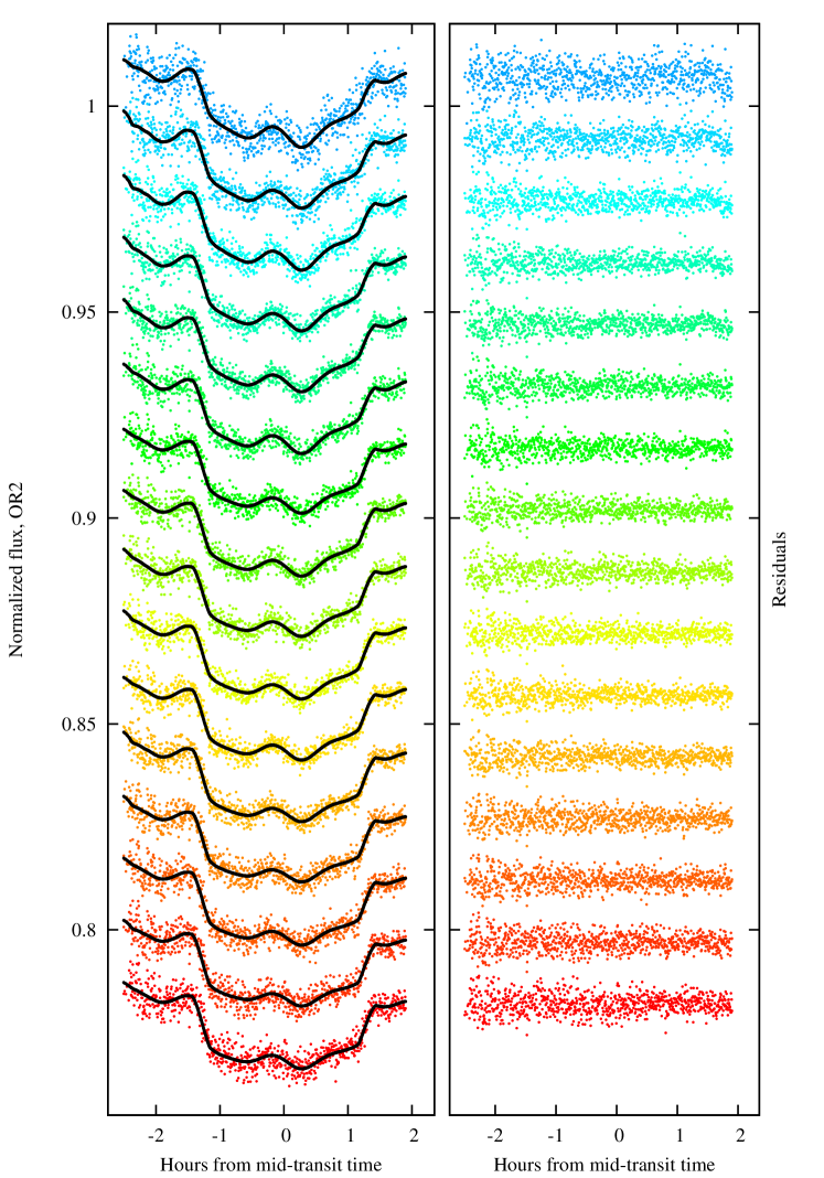
Figure 6 and Figure 7 show the chromatic light curves of WASP-33 b, shifted with respect to the best-fit mid-transit time and shown in hours. The light curves are color-coded with respect to the wavelength channel. Black continuous line shows the best-fit model, which comprises the transit, the detrending, and the pulsation models. Photometric errors are enlarged by their respective $\beta$ values. The chromatic light curves have been vertically shifted to allow for visual inspection. Table 3 specifies the wavelength channels, the derived planet-to-star radius along with their uncertainties, the limb darkening values, and the best-fit detrending coefficients.

Figure 6: Our 16 chromatic transit light curves obtained during OR1 on the left panels, and corresponding residuals on the right. The continuous black line represents our model, comprising the pulsations, the detrending, and the transit models. Transits are plotted in hours from mid-transit time, and are shifted vertically to allow for visual inspection.

Figure 7: Results obtained during OR2 (see Figure 6).

Table 3: From left to right, center of integration band and integration width, best fit planet-to-star radius ratio, detrending coefficients $\mathrm{c_{0}}$, $\mathrm{c_{1}}$, $\mathrm{c_{2}}$, and $\mathrm{c_{3}}$, standard deviation of residuals in ppt, and $\beta$ values. Best-fit values are given with 1-$\sigma$ uncertainties.

$\lambda_{o}\pm\Delta\lambda$ (nm)	$\mathrm{R_{P}/R_{s}}$	$\mathrm{c_{0}}$	$\mathrm{c_{1}}$	$\mathrm{c_{2}}$	$\mathrm{c_{3}}$	$\sigma$ (ppt)	$\beta$
OR1
430.3 $\pm$ 10.3	0.1082 $\pm$ 0.0014	1.0091 $\pm$ 0.0003	0.025 $\pm$ 0.003	-0.020 $\pm$ 0.004	-0.67 $\pm$ 0.09	2.4	1.63
450.9 $\pm$ 10.3	0.1070 $\pm$ 0.0012	1.0085 $\pm$ 0.0003	0.015 $\pm$ 0.002	-0.012 $\pm$ 0.003	-0.50 $\pm$ 0.07	2.0	1.69
471.6 $\pm$ 10.3	0.1073 $\pm$ 0.0009	1.0085 $\pm$ 0.0002	0.007 $\pm$ 0.002	-0.009 $\pm$ 0.003	-0.35 $\pm$ 0.06	1.6	1.66
492.2 $\pm$ 10.3	0.1080 $\pm$ 0.0009	1.0083 $\pm$ 0.0002	0.003 $\pm$ 0.002	-0.006 $\pm$ 0.002	-0.24 $\pm$ 0.05	1.5	1.15
512.8 $\pm$ 10.3	0.1067 $\pm$ 0.0009	1.0082 $\pm$ 0.0002	0.000 $\pm$ 0.002	-0.007 $\pm$ 0.002	-0.17 $\pm$ 0.05	1.5	1.37
533.4 $\pm$ 10.3	0.1067 $\pm$ 0.0008	1.0084 $\pm$ 0.0002	0.000 $\pm$ 0.002	-0.011 $\pm$ 0.002	-0.21 $\pm$ 0.05	1.4	1.28
554.1 $\pm$ 10.3	0.1057 $\pm$ 0.0009	1.0080 $\pm$ 0.0002	-0.004 $\pm$ 0.002	-0.005 $\pm$ 0.002	-0.10 $\pm$ 0.05	1.5	1.01
574.7 $\pm$ 10.3	0.1048 $\pm$ 0.0009	1.0075 $\pm$ 0.0002	-0.010 $\pm$ 0.002	0.001 $\pm$ 0.002	0.04 $\pm$ 0.05	1.4	1.20
595.3 $\pm$ 10.3	0.1037 $\pm$ 0.0009	1.0076 $\pm$ 0.0002	-0.004 $\pm$ 0.002	-0.003 $\pm$ 0.002	-0.09 $\pm$ 0.05	1.5	1.05
615.9 $\pm$ 10.3	0.1060 $\pm$ 0.0009	1.0078 $\pm$ 0.0002	-0.006 $\pm$ 0.002	-0.002 $\pm$ 0.002	-0.02 $\pm$ 0.05	1.5	1.06
636.6 $\pm$ 10.3	0.1041 $\pm$ 0.0009	1.0074 $\pm$ 0.0002	-0.004 $\pm$ 0.002	0.001 $\pm$ 0.002	-0.13 $\pm$ 0.05	1.5	1.07
657.2 $\pm$ 10.3	0.1048 $\pm$ 0.0009	1.0073 $\pm$ 0.0002	-0.003 $\pm$ 0.002	0.002 $\pm$ 0.002	-0.13 $\pm$ 0.05	1.4	1.07
677.8 $\pm$ 10.3	0.1049 $\pm$ 0.0009	1.0075 $\pm$ 0.0002	-0.002 $\pm$ 0.002	-0.001 $\pm$ 0.002	-0.18 $\pm$ 0.05	1.4	1.08
698.4 $\pm$ 10.3	0.1043 $\pm$ 0.0009	1.0072 $\pm$ 0.0002	-0.002 $\pm$ 0.002	0.004 $\pm$ 0.002	-0.23 $\pm$ 0.05	1.5	1.12
719.1 $\pm$ 10.3	0.1057 $\pm$ 0.0009	1.0076 $\pm$ 0.0002	0.001 $\pm$ 0.002	-0.001 $\pm$ 0.002	-0.33 $\pm$ 0.05	1.5	1.11
739.7 $\pm$ 10.3	0.1055 $\pm$ 0.0009	1.0076 $\pm$ 0.0002	0.002 $\pm$ 0.002	-0.004 $\pm$ 0.002	-0.39 $\pm$ 0.05	1.6	1.06
OR2
530.5 $\pm$ 10.5	0.1046 $\pm$ 0.0021	1.0061 $\pm$ 0.0003	0.010 $\pm$ 0.005	0.010 $\pm$ 0.003	-0.58 $\pm$ 0.65	3.0	1.16
551.4 $\pm$ 10.5	0.1037 $\pm$ 0.0013	1.0060 $\pm$ 0.0003	0.016 $\pm$ 0.004	0.016 $\pm$ 0.003	-1.31 $\pm$ 0.54	2.4	1.03
572.3 $\pm$ 10.5	0.1037 $\pm$ 0.0013	1.0061 $\pm$ 0.0003	0.014 $\pm$ 0.004	0.014 $\pm$ 0.003	-1.20 $\pm$ 0.56	2.1	1.05
593.2 $\pm$ 10.5	0.1044 $\pm$ 0.0012	1.0060 $\pm$ 0.0002	0.019 $\pm$ 0.004	0.019 $\pm$ 0.003	-0.74 $\pm$ 0.51	1.9	1.06
614.1 $\pm$ 10.5	0.1043 $\pm$ 0.0012	1.0060 $\pm$ 0.0002	0.018 $\pm$ 0.004	0.018 $\pm$ 0.003	-0.79 $\pm$ 0.57	1.8	1.04
635.0 $\pm$ 10.5	0.1033 $\pm$ 0.0012	1.0059 $\pm$ 0.0002	0.016 $\pm$ 0.004	0.016 $\pm$ 0.003	-0.43 $\pm$ 0.48	1.8	1.26
655.9 $\pm$ 10.5	0.1049 $\pm$ 0.0012	1.0063 $\pm$ 0.0002	0.013 $\pm$ 0.004	0.013 $\pm$ 0.003	-0.27 $\pm$ 0.52	1.8	1.05
676.8 $\pm$ 10.5	0.1063 $\pm$ 0.0011	1.0064 $\pm$ 0.0002	0.016 $\pm$ 0.004	0.016 $\pm$ 0.002	-0.26 $\pm$ 0.52	1.7	1.05
697.7 $\pm$ 10.5	0.1044 $\pm$ 0.0012	1.0060 $\pm$ 0.0002	0.019 $\pm$ 0.004	0.019 $\pm$ 0.003	-0.36 $\pm$ 0.50	1.8	1.01
718.6 $\pm$ 10.5	0.1072 $\pm$ 0.0011	1.0064 $\pm$ 0.0002	0.016 $\pm$ 0.004	0.016 $\pm$ 0.003	-0.59 $\pm$ 0.50	1.7	1.08
739.5 $\pm$ 10.5	0.1058 $\pm$ 0.0011	1.0062 $\pm$ 0.0002	0.015 $\pm$ 0.004	0.015 $\pm$ 0.003	-0.28 $\pm$ 0.52	1.7	1.07
781.0 $\pm$ 11.0	0.1073 $\pm$ 0.0012	1.0065 $\pm$ 0.0002	0.014 $\pm$ 0.004	0.014 $\pm$ 0.003	-0.79 $\pm$ 0.52	1.7	1.09
803.0 $\pm$ 11.0	0.1054 $\pm$ 0.0012	1.0062 $\pm$ 0.0002	0.013 $\pm$ 0.004	0.013 $\pm$ 0.003	-0.64 $\pm$ 0.54	1.9	1.03
825.0 $\pm$ 11.0	0.1069 $\pm$ 0.0012	1.0065 $\pm$ 0.0002	0.011 $\pm$ 0.004	0.011 $\pm$ 0.003	-0.25 $\pm$ 0.49	1.9	1.05
847.0 $\pm$ 11.0	0.1078 $\pm$ 0.0013	1.0067 $\pm$ 0.0003	0.010 $\pm$ 0.004	0.010 $\pm$ 0.003	-0.61 $\pm$ 0.50	2.0	1.04
869.0 $\pm$ 11.0	0.1082 $\pm$ 0.0013	1.0066 $\pm$ 0.0003	0.011 $\pm$ 0.004	0.011 $\pm$ 0.003	-0.19 $\pm$ 0.58	2.3	1.39

3.8 Consistency checkup of our results

We identify three critical components of our model and model strategy that might have an effect on the derived transmission spectrum of WASP-33 b. These are the selection of particular detrending components, the specific integration bandwidths, and the particular way we treat the pulsations.

To investigate the impact of the choice of detrending model into the determination of the transmission spectrum of WASP-33 b, we carried out the same procedure but as for the detrending models, we considered the following:

1. A first order, time-dependent polynomial,
   DM(t) = $c_{0}$ + $c_{1}$t.

2. A second order, time-dependent polynomial,
   DM(t) = $c_{0}$ + $c_{1}$t + $c_{2}$t².

3. A linear relation with airmass and background,
   DM($\chi$, bc) = $c_{0}$ + $c_{1}\chi$ + $c_{2}$bg.

4. A linear relation with airmass, and quadratic with background,
   DM($\chi$, bc) = $c_{0}$ + $c_{1}\chi$ + $c_{2}$bc + $c_{3}$bc².

5. A quadratic relation with airmass,
   DM($\chi$) = $c_{0}$ + $c_{1}\chi$ + $c_{2}\chi^{2}$.

To investigate if the choice of integration bandwidth has an impact in the transmission spectrum of WASP-33 b, we changed their width and re-computed new light curves. For each detrending function and choice of bandwidth, we fitted the chromatic light curves in the exact same fashion as described in previous sections.

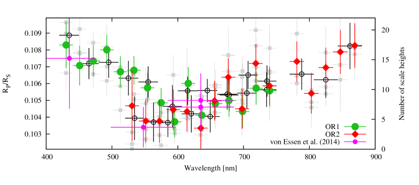
Our results are shown in Figure 8. The green circles and red diamonds correspond to the OR1 and OR2, respectively. Over-plotted as gray squares and black empty circles we show the results derived from different detrending components and bandwidths, respectively. Pink filled circles show values reported in von Essen et al. (2014). As the figure shows, our results are fully consistent at 1-$\sigma$ uncertainties. In addition, similarly to von Essen et al. (2015) we also considered additional models for the stellar pulsations, included in our data analysis considering the following changes:

1. Eight frequencies fitted with Gaussian priors, using our best-fit values from von Essen et al. (2014) and their respective errors as mean and standard deviations for the priors.

2. A unique set of eight phases for the two transits, fitted to the data with uniform priors.

3. A unique set of planet-to-star radius ratio for each wavelength bin where the two transits coincide.

4. A unique set of amplitude offsets for each wavelength bin where the two transits coincide.

5. Two sets of phases with uniform priors.

Figure 8: Transmission spectrum of WASP-33 b. Green circles and red diamonds correspond to the planet-to-star radius ratio obtained from OR1 and OR2, respectively. Gray light squares are derived fitting different detrending components to the data. Pink filled circles are from von Essen et al. (2014), and open black circles are considering larger integration bins. In all cases, error bars are at 1-$\sigma$ level and horizontal lines indicate the size of the wavelength bin.

In this analysis, point 1. returned consistent results for $\mathrm{R_{P}/R_{S}}$ but with slightly larger error bars. So did points 2. and 3., but with slightly smaller error bars where the wavelengths coincided. A visual inspection of the residuals obtained from point 4. repeated systematically using different detrending functions showed clear signs of pulsations not properly accounted for. For example, when fitting the two white light curves with two set of phases, as stated in previous sections the derived beta-values were $\beta_{OR1}$ = 1.05, and $\beta_{OR2}$ = 1.29. After considering one set of phases and recomputing the beta-values, we obtained $\beta_{OR1,min}$ = 1.74, $\beta_{OR1,max}$ = 6.93, $\beta_{OR2,min}$ = 2.16, and $\beta_{OR2,max}$ = 7.03 as minimum and maximum values of our best-fit models. The corresponding BIC values were in all cases larger than 1700. This supports the need for the two sets of phases.

4 Transmission spectrum of WASP-33 b

4.1 Atmospheric retrieval

We performed an atmospheric retrieval on the combined spectrum of WASP-33b to constrain the atmospheric properties at the day-night terminator region. We employed an atmospheric retrieval code for transit spectroscopy adapted from the recent work of Gandhi & Madhusudhan (2018). Our code computes line-by-line radiative transfer in a transmission geometry and assumes a plane parallel planetary atmosphere in hydrostatic equilibrium. The model parametrizes the pressure-temperature profile of the atmosphere using the prescription of Madhusudhan & Seager (2009) containing six free parameters. The volumetric mixing ratios of the chemical species in the atmosphere are also free parameters in the retrieval framework. We employed chemical opacities adopted from the work of Gandhi & Madhusudhan (2017, 2018). Our models consider molecules, metal oxides and hydrides, and atomic species that could be present in hot Jupiter atmospheres: H₂O, CO, CH₄, NH₃, CO₂, TiO, AlO, VO, FeH, TiH, CrH, Na, and K (Madhusudhan et al., 2016b).

Furthermore, our model considers inhomogeneous cloud coverage and scattering hazes. Our model considers cloudy regions of the atmosphere to consist of an opaque cloud deck at pressures larger than P${}_{\text{c}}$ in units of bar and scattering due to hazes above the clouds. We employed the cloud and haze parametrization of MacDonald & Madhusudhan (2017) in which the haze component is included as $\sigma=a\sigma_{0}(\lambda/\lambda_{0})^{\gamma}$, where $\gamma$ is the scattering slope, $a$ is the Rayleigh-enhancement factor, and $\sigma_{0}$ is the H₂ Rayleigh scattering cross-section ($5.31\times 10^{-31}$ m²) at the reference wavelength $\lambda_{0}=350$ nm. For the consideration of inhomogeneous clouds and scattering hazes, the parameter $\bar{\phi}$ is the cloud and haze fraction cover in the planet’s atmosphere. The retrieval framework allows for the possibility of a flat spectrum (e.g., due to weak gaseous absorption and/or a gray homogeneous cloud cover) in the explored parameter space. Parameter estimation and Bayesian model comparisons are performed using MultiNest (Feroz et al., 2009) through the Python interface PyMultiNest (Buchner et al., 2014).

Figure 9: Transmission spectrum of WASP-33b and retrieved models. The blue and black circles represent transit depths from OR1 and OR2, respectively. Horizontal lines indicate the size of the wavelength bin. Error bars are at the 1-$\sigma$ level. The red curve shows the retrieved median model and the 1-$\sigma$ and 2-$\sigma$ confidence envelopes are shown by the shaded regions. The gold diamonds show the binned median model at the same resolution as the data. The spectrum shows a feature from $\sim$450$-$550 nm that is explained by the model spectrum including AlO.

Table 4: Bayesian model comparison detection of atmospheric compositions at the terminator of WASP-33b.

Model	Evidence	Bayes factor	Detection
	$\ln(\mathcal{Z})$	$\mathcal{B}_{0i}$	of Ref.
Reference	215.1	Ref.	Ref.
No AlO	211.3	46.7	3.28-$\sigma$
Flat line model	208.0	1232.3	4.18-$\sigma$
No hazes/clouds	215.8	0.5	N/A

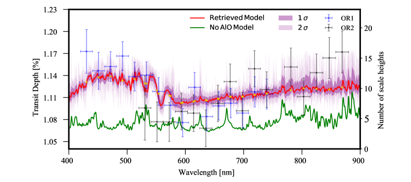
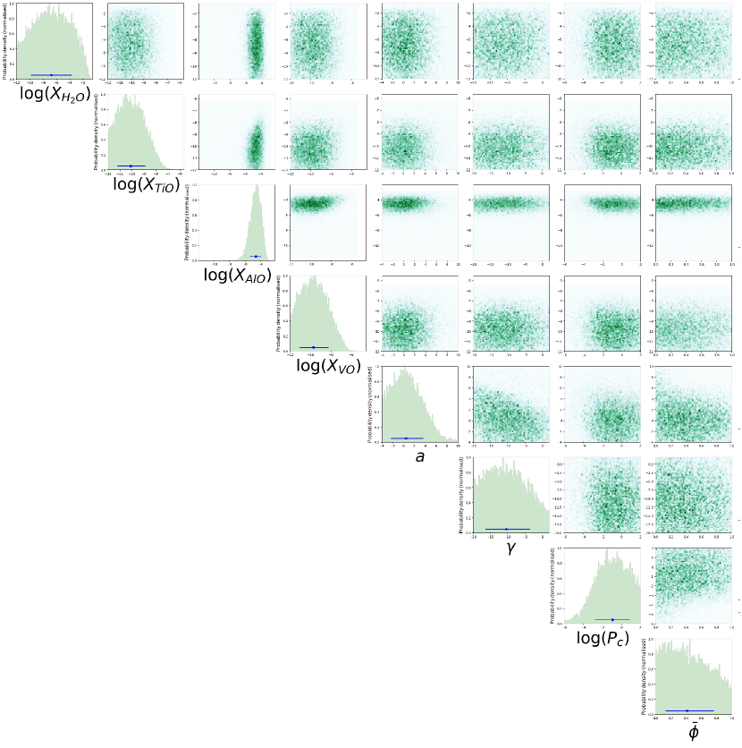
The analysis of the transmission spectrum of WASP-33b provides initial constraints on its atmospheric composition. Figure 9 shows the retrieved median fit to the observations along with the 1-$\sigma$ and 2-$\sigma$ confidence contours. In particular, we report a possible detection of AlO at 3.3-$\sigma$ significance as shown in Table 4. We retrieve a volume mixing ratio of $\log(X_{\mathrm{AlO}})=-4.58^{+0.67}_{-0.79}$ for AlO. Although we do not find statistically significant evidence for the other species considered in our retrieval, the upper limits at the 99th percentile for TiO and VO are $\log(X_{\mathrm{TiO}})=-7.52$ and $\log(X_{\mathrm{VO}})=-6.74$. Although water vapor was considered in our models, the long-wavelength data do not show any features corresponding to H₂O absorption. Models without AlO fail to explain the features from 450-550 nm, as can be seen in Fig. 9.

We used Bayesian model comparisons to evaluate the detection significance of AlO as shown in Table 4. We find that our full 28-parameter model with AlO is preferred over a 27-parameter model without AlO at a 3.3-$\sigma$ significance. We also investigated fits to the data with a featureless spectrum represented by a constant transit depth, that is, a one-parameter flat line model, using MultiNest. We find that the full 28-parameter model is preferred over the one-parameter flat spectrum model at 4.2-$\sigma$ significance. We present the Bayesian evidence and model comparisons in Table 4.

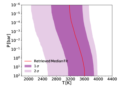
The retrieved pressure-temperature profile is shown in Figure 10. We obtain a relatively unconstrained profile consistent with the equilibrium temperature of $T_{eq}\sim$2700 K, reported in Smith et al. (2011), within the 2-$\sigma$ region. The retrieved median fit for the $P$-$T$ profile varies from $\sim$3200 K at the top of the atmosphere to $\sim$3600 K at the 1-bar surface. The retrieved $P$-$T$ profile is also consistent with the average dayside brightness temperature of 3144 $\pm$ 114 K in the near-infrared reported in Zhang et al. (2018). Transmission spectra probe the day-night terminator region, sampling temperatures of both the dayside and nightside of the atmosphere. Furthermore, transmission spectra in the optical probe higher regions in the atmosphere than emission spectra. If WASP-33b has a thermal inversion (e.g., Haynes et al., 2015) it is conceivable that the upper atmosphere probed by a transmission spectrum may be comparable in temperature to that of the dayside photosphere reported by Zhang et al. (2018). Our model considers the presence of clouds and hazes in the atmosphere of WASP-33b. However, the data does not constrain the cloud and haze properties of the planet. The data in the optical wavelengths lacks features indicative of a scattering slope. We performed a retrieval test for a clear atmosphere and the molecular abundances remained unchanged. A clear atmosphere is consistent with studies showing that the condensation temperatures of expected cloud- and haze-forming species are well below that of WASP-33b (Pinhas & Madhusudhan, 2017; Wakeford et al., 2017). The posterior distributions for the relevant parameters are shown in Figure 11.

Our detection significance for AlO of 3.3-$\sigma$ represents a conservative limit. Given the large number of model parameters used for completeness in our full retrieval the evidence, and hence the significance, is conservative. In practice, several of the 28 model parameters do not contribute significantly in the observed visible band. Retrieval with a model considering only the parameters that affect the visible spectrum constitute a more meaningful measure of the detection significance. To further test the significance of the AlO detection we consider an additional simplified retrieval. Given that our full retrieval was not able to constrain the cloud properties of WASP-33b or the P-T profile, our simplified model is a clear atmosphere with absorption from TiO and AlO only, and an isothermal temperature profile, that is, four free parameters. The resulting retrieval obtains a log evidence of 217.7. Using this four-parameter model with AlO as our reference in a Bayesian model comparison, we estimate its detection significance relative to models without AlO. We find that the reference model is preferred over a three-parameter model without AlO at 4.7-$\sigma$ significance. Similarly, the reference models is preferred over a one-parameter flat line model at 4.8-$\sigma$ significance. Although this analysis suggests that our detection of AlO is at a confidence level higher than 3.3-$\sigma$, we still adopt the more conservative detection significance obtained using the full 28-parameter model.

Our retrieved AlO abundance constrains the Al/H ratio in the atmosphere. The volume mixing ratio of $\log(X_{\mathrm{AlO}})=-4.58^{+0.67}_{-0.79}$ corresponds to an abundance of $\log(\mathrm{AlO/H})=-4.81^{+0.67}_{-0.79}$. Assuming all the Al is contained in AlO, our derived estimate of Al/H is consistent with a solar value of $\log(\mathrm{Al/H})=-5.55\pm 0.03$ (Asplund et al., 2009). However, Al can also be present in other refractory species, in which case our derived estimate is a lower limit on the true Al/H abundance in the atmosphere of WASP-33b. In particular, the dominant Al-containing species in a solar-composition atmosphere in equilibrium, at temperatures near 3000 K, include Al and AlH (Woitke et al., 2018). Under such conditions, our retrieved AlO abundance is $\sim$ 10³ $\times$ higher than that predicted in chemical equilibrium with solar abundances. Future studies may investigate the feasibility of our retrieved abundance of AlO in WASP-33b, possibly due to chemical disequilibrium or other mechanisms. Future observations may also provide better constraints on the same.

Figure 10: Retrieved temperature structure along the planetary limb. The retrieved median profile is shown in red and the 1-$\sigma$ and 2-$\sigma$ confidence intervals are shown as the shaded areas.

Figure 11: Marginalized posterior probability densities for the detected molecule (AlO) and the molecules for which upper bounds have been determined (TiO and VO), along with the cloud and haze parameters. The posterior distribution for water is included for reference.

4.2 The aluminum oxide feature

The main spectral feature of the optical transmission spectrum reported in this work is an increase in the planet-star radius ratio blueward of about 560 nm. In general, an increase toward short wavelengths can be caused by third light of an additional stellar companion in the aperture of flux extraction. Moya et al. (2011) detected a stellar object 2 arcsec away from WASP-33, well included within our aperture. The authors estimated that the probable physical companion of WASP-33 should have an effective temperature of about $\sim$3000 K. As carried out in von Essen et al. (2015), within our wavelength region we estimated that the M dwarf should be at least $10^{3}$ times dimmer than WASP-33. This would create a variability of planet-to-star radius ratio as large as 60 ppm. This upper value is well contained within our error bars given that the median precision of the dataset is 245 ppm. Thus, it is safe to neglect the contribution of WASP-33’s companion. Also, star spots might in principle cause a spectral slope in the transmission spectrum (Sing et al., 2011; Oshagh et al., 2014). This possibility plays no role for WASP-33 either, since it has no or a too thin outer convection zone, making star spots unlikely to occur. In consequence, we have interpreted the spectral feature shortward of 560 nm as an increase in opacity in the planetary atmosphere of WASP-33 b.

In Section 4.1 we retrieved AlO as the opacity source of the spectral feature between 450 nm and 550 nm. Spectral absorption features by gaseous AlO have not been reported in the literature of exoplanet observations, though atmospheric models predict its importance in hot Jupiters (Gandhi, S., & Madhusudhan, N., 2018, MNRAS (submitted). AlO was described as a potential condensate forming clouds or hazes in very hot exoplanet atmospheres (e.g., Lodders, 2002; Wakeford et al., 2017; Pinhas & Madhusudhan, 2017). AlO is difficult to observe for M or L type stellar objects, first because the optical spectra of these low-mass stars are dominated by TiO and VO absorption features, and second because such spectral feature at $\sim$ 500 nm is challenging to observe for very late type stars because of their intrinsic faintness at these wavelengths. As for the exoplanet atmospheres, AlO is mentioned in the literature of low mass stellar objects as condensate forming species (e.g., Burrows & Sharp, 1999; Allard et al., 2011; Helling et al., 2017).

5 Conclusions

In this work we report GTC/OSIRIS low resolution spectroscopic observations of WASP-33 b carried out during two transits taken 18 orbits apart. Our combined observations cover wavelengths between 420 and 880 nm. Our main aim is to characterize the chemical composition of the atmosphere of the ultra-hot Jupiter WASP-33 b, one of the hottest exoplanets known to date. We used our previous knowledge of the pulsations of the host star to create a physical model that, besides the intrinsic variability of the host star, included the transit feature and the effects induced by our Earth’s atmosphere, along with the imperfections in the instruments collecting these data. Fitting the chromatic transit light curves simultaneously, but the pulsations and the planet-to-star radii ratios independently, allowed us to contrast our results. Within the common wavelengths, our derived transmission spectra are fully consistent within 1-$\sigma$ uncertainties. Using detailed atmospheric retrieval methods we find that the feature observed between 450 and 550 nm can be best explained by aluminum oxide in the planetary atmosphere at a detection significance of 3.3-$\sigma$. We find no significant evidence for other chemical species, but report upper limits for TiO and VO which are indicative of subsolar abundances of these species at the terminator region of WASP-33 b. The obtained transmission spectrum does not constrain the cloud and haze properties of the planet. While the data shows strong evidence for AlO, we note that the retrieved AlO abundance is $\sim$ 10³ $\times$ higher than that predicted assuming thermochemical equilibrium with solar elemental abundances. More observations of the transmission spectrum of WASP-33b in the visible, both from ground-based facilities Sedaghati et al. (2017); Chen et al. (2018) as well as with HST Sing et al. (2016), could help improve upon the present constraints.