Quantizers with Parameterized Distortion Measures

Abstract

In many quantization problems, the distortion function is given by the Euclidean metric to measure the distance of a source sample to any given reproduction point of the quantizer. We will in this work regard distortion functions, which are additively and multiplicatively weighted for each reproduction point resulting in a heterogeneous quantization problem, as used for example in deployment problems of sensor networks. Whereas, normally in such problems, the average distortion is minimized for given weights (parameters), we will optimize the quantization problem over all weights, i.e., we tune or control the distortion functions in our favor. For a uniform source distribution in one-dimension, we derive the unique minimizer, given as the uniform scalar quantizer with an optimal common weight. By numerical simulations, we demonstrate that this result extends to two-dimensions where asymptotically the parameter optimized quantizer is the hexagonal lattice with common weights. As an application, we will determine the optimal deployment of unmanned aerial vehicles (UAVs) to provide a wireless communication to ground terminals under a minimal communication power cost. Here, the optimal weights relate to the optimal flight heights of the UAVs.

I Introduction

For a set $\Omega\subset{\mathbb{R}}^{d}$ in $d=1,2$ dimensions, a quantizer is given by $N$ reproduction or quantization points $\mathbf{Q}=\{\mathbf{q}_{1},\dots,\mathbf{q}_{N}\}\subset\Omega$ associated with $N$ quantization regions $\mathcal{R}=\{\mathcal{R}_{1},\dots,\mathcal{R}_{N}\}\subset\Omega$, defining a partition of $\Omega$. To measure the quality of a given quantizer, the Euclidean distance between the source samples and reproduction points is commonly used as the distortion function. We will study quantizers with parameter depending distortion functions which minimize the average distortion over $\Omega$ for a given continuous source sample distribution $\lambda:\Omega\to[0,1]$, as investigated for example in [Erdem16, KJ17, KKSS18] with a fixed set of parameters. Contrary to a fixed parameter selection, we will assign to each quantization point variable parameters to control the distortion function of the each quantization point individually. Such controllable distortion functions widens the scope of quantization theory and allows one to apply quantization techniques to many parameter dependent network and locational problems. In this work, we will consider for the distortion function of $\mathbf{q}_{n}$ a Euclidean square-distance, which is multiplicatively weighted by some $a_{n}>0$ and additively weighted by some $b_{n}>0$. Furthermore, we exponentially weight all distortion functions by some fixed exponent $\gamma\geq 1$. To minimize the average distortion, the optimal quantization regions are known to be generalized Voronoi (Möbius) regions, which can be non-convex and disconnected sets [BWY07]. In many applications, as in sensor or vehicle deployments, the optimal weights and parameters are usually unknown, but adjustable, and one wishes therefore to optimize the deployment over all admissible parameter values, see for example [ML]. We will characterize such quantizers with parameterized distortion measures over one-dimensional convex target regions, i.e., over closed intervals. As a motivation, we will demonstrate such a parameter driven quantizer for an unmanned aerial vehicle (UAV) deployment to provide energy-efficient communication to ground terminals in a given target region $\Omega$. Here, the parameters relate to the UAVs flight heights.

Notation

By $[N]=\{1,2,\dots,N\}$ we denote the first $N$ natural numbers, ${\mathbb{N}}$. We will write real numbers in ${\mathbb{R}}$ by small letters and row vectors by bold letters. The Euclidean norm of ${\mathbf{x}}$ is given by $\left\|{\mathbf{x}}\right\|=\sqrt{\sum_{n}x_{n}^{2}}$. The open ball in ${\mathbb{R}}^{d}$ centered at ${\mathbf{c}}\in{\mathbb{R}}^{d}$ with radius $r\geq 0$ is denoted by $\mathcal{B}\left({\mathbf{c}},r\right)=\left\{\left.\boldsymbol{\omega}\rule[-2.5pt]{0.0pt}{11.80444pt}\;\right|\;\|\boldsymbol{\omega}-{\mathbf{c}}\|^{2}\leq r\right\}$. We denote by $\mathcal{V}^{c}$ the complement of the set $\mathcal{V}\subset{\mathbb{R}}^{d}$. The positive real numbers are denoted by ${\mathbb{R}}_{+}:=\left\{\left.a\in{\mathbb{R}}\rule[-0.39098pt]{0.0pt}{6.83542pt}\;\right|\;a>0\right\}$. Moreover, for two points ${\mathbf{a}},{\mathbf{b}}\in{\mathbb{R}}^{d}$, we denote the generated half space between them, which contains ${\mathbf{a}}\in{\mathbb{R}}^{d}$, as $\mathcal{H}({\mathbf{a}},{\mathbf{b}})$.

II System model

To motivate the concept of parameterized distortion measures, we will investigate the deployment of $N$ UAVs positioned at $\mathbf{P}=\{\mathbf{p}_{1},\dots,\mathbf{p}_{N}\}\subset(\Omega\times{\mathbb{R}}_{+})^{N}$ to provide a wireless communication link to ground terminals (GTs) in a given target region $\Omega\subset{\mathbb{R}}^{d}$. Here, the $n$th UAV’s position, $\mathbf{p}_{n}=(\mathbf{q}_{n},h_{n})$, is given by its ground position $\mathbf{q}_{n}=(x_{n},y_{n})\in\Omega$, representing the quantization point, and its flight height $h_{n}$, representing its distortion parameter. The optimal UAV deployment is then defined by the minimum average communication power (distortion) to serve GTs distributed by a density function $\lambda$ in $\Omega$ with a minimum given data rate $R_{b}$. Hereby, each GT will select the UAV which requires the smallest communication power, resulting in so called generalized Voronoi (quantization) regions of $\Omega$, as used in [Erdem16, GJ, GJcom18, GJ18, KJ17, ML, MLCS, KKSS18]. We also assume that the communication between all users and UAVs is orthogonal, i.e., separated in frequency or time (slotted protocols).

In the recent decade, UAVs with directional antennas have been widely studied in the literature [BJL, MSF, HA, KMR, HSYR, MWMM], to increase the efficiency of wireless links. However, in [BJL, MSF, HA, KMR, HSYR, MWMM], the antenna gain was approximated by a constant within a 3dB beamwidth and set to zero outside. This ignores the strong angle-dependent gain of directional antennas, notably for low-altitude UAVs. To obtain a more realistic model, we will consider an antenna gain which depends on the actual radiation angle $\theta_{n}\in[0,\frac{\pi}{2}]$ from the $n$th UAV at $\mathbf{p}_{n}$ to a GT at $\boldsymbol{\omega}$, see Fig. (1). To capture the power falloff versus the line-of-sight distance $d_{n}$ along with the random attenuation and the path-loss, we adopt the following propagation model [Gol05, (2.51)]

$$PL_{dB}=10\log_{10}{K}-10\alpha\log_{10}(d_{n}/d_{0})-\psi_{dB},$$ (1)

where $K$ is a unitless constant depending on the antenna characteristics, $d_{0}$ is a reference distance, $\alpha\geq 1$ is the terrestrial path-loss exponent, and $\psi_{dB}$ is a Gaussian random variable following $\mathcal{N}\left(0,\sigma^{2}_{\psi_{dB}}\right)$. This air-to-ground or terrestrial path-loss model is widely used for UAV basestations path-loss models [MSBD16a]. Practical values of $\alpha$ are between $2$ and $6$ and depend on the Euclidean distance of GT $\boldsymbol{\omega}$ and UAV $\mathbf{p}_{n}$

$$d_{n}(\boldsymbol{\omega})=d(\mathbf{p}_{n},(\boldsymbol{\omega},0))=\sqrt{\|\mathbf{q}_{n}-\boldsymbol{\omega}\|^{2}+h_{n}^{2}}=\sqrt{(x_{n}-x)^{2}+(y_{n}-y)^{2}+h_{n}^{2}}.$$ (2)

For common practical measurements, see for example [AG18]. Typically maximal heights for UAVs are $<1000$m, due to flight zone restrictions of aircrafts. Hence, the received power at UAV $n$ can be represented as $P_{RX}=P_{TX}G_{TX}G_{RX}Kd^{\alpha}_{0}d_{n}^{-\alpha}(\boldsymbol{\omega})10^{-\frac{\psi_{dB}}{10}}$, where $G_{TX}$ and $G_{RX}$ are the antenna gains of the transmitter and the receiver, respectively. Here, we assume perfect omnidirectional transmitter GT antennas with an isotropic gain and directional receiver UAV antennas. The angle dependent antenna gains are

$$G_{\text{GT}}>0\quad,\quad G_{\text{UAV}}=\cos\left(\theta_{n}\right)=h_{n}/d_{n}(\boldsymbol{\omega}),$$ (3)

see [Bal05a, p.52]. The combined antenna intensity is then proportional to $G=G_{\text{UAV}}G_{\text{GT}}K$, see Fig. (1).

Figure 1: UAV deployment with directed antenna beam and associated GT cells for $\alpha=2$ and $N=2$ for a uniform GT distribution.

Accordingly, the received power can be rewritten as

$$P_{RX}=P_{TX}h_{n}G_{\text{GT}}Kd^{\alpha}_{0}d_{n}^{-\alpha-1}(\boldsymbol{\omega})10^{-\frac{\psi_{dB}}{10}}.$$ (4)

To achieve a reliable communication between GT and UAV with bit-rate at least $R_{b}$ for a channel bandwidth $B$ and noise power density $N_{0}$, the Shannon formula requires $B\log_{2}\left(1+\frac{P_{RX}}{BN_{0}}\right)\geq R_{b}$. The minimum transmission power to UAV $\mathbf{p}_{n}$ is then given by

$$P_{TX}=\big{(}2^{\frac{R_{b}}{B}}\!-\!1\big{)}BN_{0}d(\mathbf{p}_{n},(\boldsymbol{\omega},0))^{\alpha+1}10^{\frac{\psi_{dB}}{10}}(h_{n}G_{\text{GT}}Kd^{\alpha}_{0})^{-1}$$ (5)

with expectation

$${\mathbb{E}[P_{TX}]} \!=\!\frac{(2^{\frac{R_{b}}{B}}-1)N_{0}}{h_{n}G_{\text{GT}}Kd^{\alpha}_{0}}\frac{d_{n}^{\alpha+1}(\boldsymbol{\omega})}{\sqrt{2\pi}\sigma_{\psi_{dB}}}\int_{{\mathbb{R}}}\exp\left(\!-\frac{\psi^{2}_{dB}}{2\sigma^{2}_{\psi_{dB}}}\!+\!\ln(10)\frac{\psi_{dB}}{10}\right)\!d\psi_{dB}\!=\!\frac{\beta}{h_{n}}d_{n}^{2\gamma}(\boldsymbol{\omega})$$ (6)

where the independent and fixed parameters are given by

$$\beta=(2^{\frac{R_{b}}{B}}-1)BN_{0}\exp\big{(}-\frac{\sigma_{\psi_{dB}}^{2}(\ln 10)^{2}}{200}\big{)}(G_{\text{GT}}K)^{-1}d_{0}^{-\alpha}\quad\text{and}\quad\gamma=\frac{\alpha+1}{2}.$$ (7)

Since our goal is to minimize the average transmission power (6) we define the $n$th parameter distortion function as

$$D(\boldsymbol{\omega},\mathbf{q}_{n},a_{n},b_{n})=\beta\cdot\left(a_{n}\left\|\mathbf{q}_{n}-\omega\right\|_{2}^{2}+b_{n}\right)^{\gamma}$$ (8)

where $a_{n}=h_{n}^{-1/\gamma}$ and $b_{n}=h_{n}^{2-1/\gamma}$. As can be seen from (8), the distortion is a function of the parameter $h_{n}$ in addition to the distance between the reproduction point $\mathbf{q}_{n}$ and the represented point $\boldsymbol{\omega}$. From a quantization point of view, one can start with the distortion function (8) without knowing the UAV power consumption formulas in this section. This is what we will do in the next section. For simplicity, we will set from here on $\beta=1$, since it will not affect the quantizer.

III Optimizing Quantizers with parameterized distortion measures

The communication power cost (8) defines, with $h_{n}$ and fixed $\gamma\geq 1$, a parameter-dependent distortion function for $\mathbf{q}_{n}$. For a given source sample GT density $\lambda$ in $\Omega$ and UAV deployment, the average power is the average distortion for given quantization and parameter points $(\mathbf{Q},{\mathbf{h}})$ with quantization sets $\mathcal{R}=\{\mathcal{R}_{n}\}$, which is called the average distortion of the quantizer $(\mathbf{Q},{\mathbf{h}},\mathcal{R})$

$$\bar{D}(\mathbf{Q},{\mathbf{h}},\mathcal{R})=\sum_{n=1}^{N}\int_{\mathcal{R}_{n}}D(\boldsymbol{\omega},\mathbf{q}_{n},h_{n})\lambda(\boldsymbol{\omega})d\boldsymbol{\omega}.$$ (9)

The $N$ quantization sets, which minimize the average distortion for given quantization and parameter points $(\mathbf{Q},{\mathbf{h}})$, define a generalized Voronoi tessellation $\mathcal{V}=\{\mathcal{V}_{n}(\mathbf{Q},{\mathbf{h}})\}$

$$\bar{D}(\mathbf{Q},{\mathbf{h}},\mathcal{V}):=\!\int_{\Omega}\min_{n\in[N]}\left\{D(\boldsymbol{\omega},\mathbf{q}_{n},h_{n})\right\}\lambda(\boldsymbol{\omega})d\boldsymbol{\omega}=\sum_{n=1}^{N}\int_{\mathcal{V}_{n}(\mathbf{Q},{\mathbf{h}})}\!\!\!\!\!D(\boldsymbol{\omega},\mathbf{q}_{n},h_{n})\lambda(\boldsymbol{\omega})d\boldsymbol{\omega},$$ (10)

where the generalized Voronoi regions $\mathcal{V}_{n}(\mathbf{Q},{\mathbf{h}})$ are defined as the set of sample points $\boldsymbol{\omega}$ with smallest distortion to the $n$th quantization point $\mathbf{q}_{n}$ with parameter $h_{n}$. Minimizing the average distortion $\bar{D}(\mathbf{Q},{\mathbf{h}},\mathcal{V})$ over all parameter and quantization points can be seen as an $N-$facility locational-parameter optimization problem [GJ, GJcom18, GJ18, OBSC00]. By the definition of the Voronoi regions (10), this is equivalent to the minimum average distortion over all $N-$level parameter quantizers

$$\bar{D}(\mathbf{Q}^{*},{\mathbf{h}}^{*},\mathcal{V}^{*})=\min_{(\mathbf{Q},{\mathbf{h}})\in\Omega^{N}\times{\mathbb{R}}_{+}^{N}}\bar{D}(\mathbf{Q},{\mathbf{h}},\mathcal{V})=\min_{(\mathbf{Q},{\mathbf{h}})\in\Omega^{N}\times{\mathbb{R}}_{+}^{N}}\min_{\mathcal{R}=\{\mathcal{R}_{n}\}\subset\Omega}\bar{D}(\mathbf{Q},{\mathbf{h}},\mathcal{R}),$$ (11)

which we call the $N-$level parameter optimized quantizer. To find local extrema of (10) analytically, we will need that the objective function $\bar{D}$ be continuously differentiable at any point in $\Omega^{N}\times{\mathbb{R}}_{+}^{N}$, i.e., the gradient should exist and be a continuous function. Such a property was shown to be true for piecewise continuous non-decreasing distortion functions in the Euclidean metric over $\Omega^{N}$ [CMB05, Thm.2.2] and weighted Euclidean metric [GJ]. Then the necessary condition for a local extremum is the vanishing of the gradient at a critical point. First, we will derive the generalized Voronoi regions for convex sets $\Omega$ in $d$ dimensions for any parameters $h_{n}\in{\mathbb{R}}_{+}$ for the quantization points $\mathbf{q}_{n}$, which are special cases of Möbius diagrams (tessellations), introduced in [BWY07].

Lemma 1.

Let $\mathbf{Q}=\{\mathbf{q}_{1},\mathbf{q}_{2},\dots,\mathbf{q}_{N}\}\subset\Omega^{N}\subset({\mathbb{R}}^{d})^{N}$ for $d\in\{1,2\}$ be the quantization points and ${\mathbf{h}}=(h_{1},\dots,h_{N})\in{\mathbb{R}}_{+}^{N}$ the associated parameters. Then the average distortion of $(\mathbf{Q},{\mathbf{h}})$ over all samples in $\Omega$ distributed by $\lambda$ for some exponent $\gamma\geq 1$

$$\bar{D}\left(\mathbf{Q},{\mathbf{h}},\mathcal{V}\right)=\sum_{n=1}^{N}\int_{\mathcal{V}_{n}}\!\frac{(\left\|\mathbf{q}_{n}-\boldsymbol{\omega}\right\|^{2}+h_{n}^{2})^{\gamma}}{h_{n}}\lambda(\boldsymbol{\omega})d\boldsymbol{\omega}$$ (12)

has generalized Voronoi regions $\mathcal{V}_{n}=\mathcal{V}_{n}(\mathbf{Q},{\mathbf{h}})=\bigcap_{m\not=n}\mathcal{V}_{nm}$, where the dominance regions of quantization point $n$ over $m$ are given by

$$\mathcal{V}_{nm}=\Omega\cap\begin{cases}\mathcal{H}(\mathbf{q}_{n},\mathbf{q}_{m})&,h_{m}=h_{n}\\ \mathcal{B}({\mathbf{c}}_{nm},r_{nm})&,h_{n}<h_{m}\\ \mathcal{B}^{c}({\mathbf{c}}_{nm},r_{nm})&,h_{n}>h_{m}\end{cases}$$ (13)

and center and radii of the balls are given by

$${\mathbf{c}}_{nm}\!=\!\frac{\mathbf{q}_{n}-h_{nm}\mathbf{q}_{m}}{1-h_{nm}}\quad\text{and}\quad r_{nm}\!=\!\left(\frac{h_{nm}}{\left(1-h_{nm}\right)^{2}}\left\|\mathbf{q}_{n}-\mathbf{q}_{m}\right\|^{2}+h_{n}^{2}\frac{h_{nm}^{1-2\gamma}-1}{1-h_{nm}}\right)^{\frac{1}{2}}.$$ (14)

Here, we introduced the parameter ratio of the $n$th and $m$th quantization point as

$$h_{nm}=\left(h_{n}/h_{m}\right)^{\frac{1}{\gamma}}.$$ (15)

Remark. It is also possible that two quantization points are equal, but have different parameters. If the parameter ratio is very small or very large, one quantization point can become redundant, i.e., if its optimal quantization set is empty. In fact, if we optimize over all quantizer points, such a case will be excluded, which we will show for one-dimension in Lemma (3).

Proof.

The minimization of the distortion functions over $\Omega$ defines an assignment rule for a generalized Voronoi diagram $\mathcal{V}(\mathbf{Q},{\mathbf{h}})=\{\mathcal{V}_{1},\mathcal{V}_{2},\dots,\mathcal{V}_{N}\}$ where

$$\mathcal{V}_{n}=\mathcal{V}_{n}(\mathbf{Q},{\mathbf{h}}):= \left\{\left.\boldsymbol{\omega}\in\Omega\rule[-2.5pt]{0.0pt}{11.80444pt}\;\right|\;a_{n}\left\|\mathbf{q}_{n}-\boldsymbol{\omega}\right\|^{2}+b_{n}\leq a_{m}\left\|\mathbf{q}_{m}-\boldsymbol{\omega}\right\|^{2}+b_{m},m\not=n\right\}$$ (16)

is the $n$th generalized Voronoi region, see for example [OBSC00, Cha.3]. Here we denoted the weights by the positive numbers

$$a_{n}=h_{n}^{-\frac{1}{\gamma}},\quad b_{n}=h_{n}^{2-\frac{1}{\gamma}}$$ (17)

which define a Möbius diagram [BK06b, BWY07]. The bisectors of Möbius diagrams are circles or lines in ${\mathbb{R}}^{2}$ as we will show below. The $n$th Voronoi region is defined by $N-1$ inequalities, which can be written as the intersection of the $N-1$ dominance regions of $\mathbf{q}_{n}$ over $\mathbf{q}_{m}$, given by

$$\mathcal{V}_{nm}=\left\{\left.\boldsymbol{\omega}\in\Omega\rule[-2.5pt]{0.0pt}{11.80444pt}\;\right|\;a_{n}\left\|\mathbf{q}_{n}-\boldsymbol{\omega}\right\|^{2}+b_{n}\leq a_{m}\left\|\mathbf{q}_{m}-\boldsymbol{\omega}\right\|^{2}+b_{m}\right\}.$$ (18)

If $h_{n}=h_{m}$ then $a_{n}=a_{m}$ and $b_{n}=b_{m}$, such that $\mathcal{V}_{nm}=\mathcal{H}(\mathbf{q}_{n},\mathbf{q}_{m})$, the left half-space between $\mathbf{q}_{n}$ and $\mathbf{q}_{m}$. For $a_{n}>a_{m}$ we can rewrite the inequality as

$$\left\|\boldsymbol{\omega}\right\|^{2}-2\left\langle{\mathbf{c}}_{nm},\boldsymbol{\omega}\right\rangle+\frac{a_{n}^{2}\left\|\mathbf{q}_{n}\right\|^{2}\!+\!a_{m}^{2}\left\|\mathbf{q}_{m}\right\|^{2}\!-\!a_{n}a_{m}(\left\|\mathbf{q}_{n}\right\|^{2}\!+\!\left\|\mathbf{q}_{m}\right\|^{2})}{(a_{n}-a_{m})^{2}}+\frac{b_{n}-b_{m}}{a_{n}-a_{m}}\leq 0$$

where the center point is given by

$${\mathbf{c}}_{nm}=\frac{a_{n}\mathbf{q}_{n}-a_{m}\mathbf{q}_{m}}{a_{n}-a_{m}}=a_{n}\frac{\mathbf{q}_{n}-h_{nm}\mathbf{q}_{m}}{a_{n}-a_{m}}=\frac{\mathbf{q}_{n}-h_{nm}\mathbf{q}_{m}}{1-h_{nm}}$$ (19)

where we introduced the parameter ratio of the $n$th and $m$th quantization point as

$$h_{nm}:=a_{m}/a_{n}=\left(h_{n}/h_{m}\right)^{\frac{1}{\gamma}}>0.$$ (20)

If $0<a_{n}-a_{m}$, which is equivalent to $h_{n}<h_{m}$, then this defines a ball (disc) and for $h_{n}>h_{m}$ its complement. Hence we get

$$\mathcal{V}_{nm}=\begin{cases}\mathcal{B}({\mathbf{c}}_{nm},r_{nm})=\left\{\left.\boldsymbol{\omega}\in\Omega\rule[-2.5pt]{0.0pt}{10.0pt}\;\right|\;\left\|\boldsymbol{\omega}-{\mathbf{c}}_{nm}\right\|<r_{nm}\right\},&h_{n}<h_{m}\\ \mathcal{H}(\mathbf{q}_{n},\mathbf{q}_{m})=\left\{\left.\boldsymbol{\omega}\in\Omega\rule[-2.5pt]{0.0pt}{10.0pt}\;\right|\;\left\|\boldsymbol{\omega}-\mathbf{q}_{n}\right\|\leq\left\|\boldsymbol{\omega}-\mathbf{q}_{m}\right\|\right\},&h_{n}=h_{m}\\ \mathcal{B}^{c}({\mathbf{c}}_{nm},r_{nm})=\left\{\left.\boldsymbol{\omega}\in\Omega\rule[-2.5pt]{0.0pt}{10.0pt}\;\right|\;\left\|\boldsymbol{\omega}-{\mathbf{c}}_{nm}\right\|>r_{nm}\right\},&h_{n}>h_{m}\end{cases}$$ (21)

where the radius square is given by

$$r_{nm}^{2} =a_{n}a_{m}\frac{\left\|\mathbf{q}_{n}-\mathbf{q}_{m}\right\|^{2}}{(a_{n}-a_{m})^{2}}+\frac{b_{m}-b_{n}}{a_{n}-a_{m}}=\frac{a_{n}}{a_{m}}\frac{\left\|\mathbf{q}_{n}-\mathbf{q}_{m}\right\|^{2}}{(1-\frac{a_{n}}{a_{m}})^{2}}+\frac{b_{m}-b_{n}}{a_{n}-a_{m}}.$$ (22)

The second summand can be written as

$$\frac{b_{m}-b_{n}}{a_{n}-a_{m}} =\frac{h_{m}^{2-\frac{1}{\gamma}}-h_{n}^{2-\frac{1}{\gamma}}}{h_{n}^{-\frac{1}{\gamma}}-h_{m}^{-\frac{1}{\gamma}}}=\frac{h_{n}^{2}\left(\left(h_{n}/h_{m}\right)^{\frac{1}{\gamma}-2}-1\right)}{1-\left(h_{n}/h_{m}\right)^{\frac{1}{\gamma}}}=h_{n}^{2}\frac{h_{nm}^{-\alpha}-1}{1-h_{nm}}.$$ (23)

For any $\gamma\geq 1$, we have $h_{nm}=(h_{n}/h_{m})^{1/\gamma}<1$ if $h_{n}<h_{m}$ and $h_{nm}\geq 1$ else. In both cases (23) is positive, which implies a radius $r_{nm}>0$ whenever $\mathbf{q}_{n}\not=\mathbf{q}_{m}$. Inserting (23) in (22) yields the result.  

Example 1. We plotted in Fig. (1), for $N=2$ and $\Omega=[0,1]^{2}$, the GT regions for a uniform distribution with UAVs placed on

$$\mathbf{q}_{1}=(0.1,0.2),h_{1}=0.5,\quad\text{and}\quad\mathbf{q}_{2}=(0.6,0.6),h_{2}=1.$$ (24)

If the second UAV reaches an altitude of $h_{2}\geq 2.3$, its Voronoi region $\mathcal{V}_{2}=\mathcal{V}_{2,1}$ will be empty and hence become “inactive“.

III-A Local optimality conditions

To find the optimal $N-$level parameter quantizer (10), we have to minimize the average distortion (9) over all possible quantization-parameter points, i.e., we have to solve a non-convex $N-$facility locational-parameter optimization problem,

$$\bar{D}(\mathbf{Q}^{*},{\mathbf{h}}^{*},\mathcal{V}^{*})=\min_{\mathbf{Q}\in\Omega^{N},{\mathbf{h}}\in{\mathbb{R}}_{+}^{N}}\sum_{n=1}^{N}\int_{\mathcal{V}_{n}(\mathbf{Q},{\mathbf{h}})}h_{n}^{-1}(\left\|\mathbf{q}_{n}-\boldsymbol{\omega}\right\|^{2}+h_{n}^{2})^{\gamma}\lambda(\boldsymbol{\omega})d\boldsymbol{\omega}$$ (25)

where $\mathcal{V}_{n}(\mathbf{Q},{\mathbf{h}})$ are the Möbius regions given in (13) for each fixed $(\mathbf{Q},{\mathbf{h}})$. A point $(\mathbf{Q}^{*},{\mathbf{h}}^{*})$ with Möbius diagram $\mathcal{V}^{*}=\mathcal{V}(\mathbf{Q}^{*},{\mathbf{h}}^{*})=\{\mathcal{V}_{1}^{*},\dots,\mathcal{V}^{*}_{N}\}$ is a critical point of (25) if all partial derivatives of $\bar{D}$ are vanishing, i.e., if for each $n\in[N]$ it holds

$$0 =\int_{\mathcal{V}^{*}_{n}}(\mathbf{q}^{*}_{n}-\boldsymbol{\omega})(\left\|\mathbf{q}^{*}_{n}-\boldsymbol{\omega}\right\|^{2}+h_{n}^{*2})^{\gamma-1}\lambda(\boldsymbol{\omega})d\boldsymbol{\omega}$$ (26)

$$0 =\int_{\mathcal{V}^{*}_{n}}(\left\|\mathbf{q}^{*}_{n}-\boldsymbol{\omega}\right\|^{2}+h_{n}^{*2})^{\gamma-1}\cdot(\left\|\mathbf{q}_{n}^{*}-\boldsymbol{\omega}\right\|^{2}-(2\gamma-1)h_{n}^{*2})\lambda(\boldsymbol{\omega})d\boldsymbol{\omega}.$$ (27)

For $N=1$ the integral regions will not depend on $\mathbf{Q}$ or ${\mathbf{h}}$ and since the integral kernel is continuous differentiable, the partial derivatives will only apply to the integral kernel. For $N>1$, the conservation-of-mass law, can be used to show that the derivatives of the integral domains will cancel each other out, see also [CMB05].

Remark. The shape of the regions depend on the parameters, which if different for each quantization point (heterogeneous), generate spherical and not polyhedral regions. We will show later, that homogeneous parameter selection with polyhedral regions will be the optimal regions for $d=1$.

III-B The optimal $N-$level parameter quantizer in one-dimension for uniform density

In this section, we discuss the parameter optimized quantizer for a one-dimensional convex source $\Omega\subset{\mathbb{R}}$, i.e., for an interval $\Omega=[s,t]$ given by some real numbers $s<t$. Under such circumstances, the quantization points are degenerated to scalars, i.e., $\mathbf{q}_{n}=x_{n}\in[s,t],\;\forall\;n\in[N]$. If we shift the interval $\Omega$ by an arbitrary $a\in{\mathbb{R}}$, then the average distortion, i.e., the objective function, will not change if we shift all quantization points by the same number $a$. Hence, if we set $a=-s$, we can shift any quantizer for $[s,t]$ to $[0,A]$ where $A=t-s$ without loss of generality. Let us assume a uniform distribution on $\Omega$, i.e. $\lambda(\omega)=1/A$. To derive the unique $N-$level parameter optimized quantizer for any $N$, we will first investigate the case $N=1$.

Lemma 2.

Let $A>0$ and $\gamma\geq 1$. The unique $1-$level parameter optimized quantizer $(x^{*},h^{*})$ with distortion function (8) is given for a uniform source density in $[0,A]$ by

$$x^{*}\!=\!\frac{A}{2},h^{*}\!=\!\frac{A}{2}g(\gamma)\quad\text{and the minimum average distortion}\quad\bar{D}(x^{*},h^{*})\!=\!\left(\frac{A}{2}\right)^{\!2\gamma-1}\!\!\!\!g(\gamma)$$

where $g(\gamma)=\arg\min_{u>0}F(u,\gamma)<1/\sqrt{2\gamma-1}$ is the unique minimizer of

$$F(u,\gamma)=\int_{0}^{1}f(\omega,u,\gamma)d\omega\quad\text{with}\quad f(\omega,u,\gamma)=\frac{(\omega^{2}+u^{2})^{\gamma}}{u}$$ (28)

which is for fixed $\gamma$ a continuous and convex function over ${\mathbb{R}}_{+}$. For $\gamma\in\{1,2,3\}$ the minimizer can be derived in closed form as

$$g(1)=\sqrt{1/3},\ \ g(2)=\sqrt{(\sqrt{32/5}-1)/9},\ \ g(3)=\sqrt{\Big{(}(32/7)^{1/3}-1\Big{)}/5}.$$ (29)

Proof.

See Appendix (A).  

Remark. The convexity of $F(\cdot,\gamma)$ can be also shown by using extensions of the Hermite-Hadamard inequality [ZC10], which allows to show convexity over any interval. Let us note here that for any fixed parameter $h_{n}>0$, the average distortion $\bar{D}(x_{n}^{*}\pm\epsilon,h_{n})$ is strictly monotone increasing in $\epsilon>0$. Hence, $x_{n}^{*}$ is the unique minimizer for any $h_{n}>0$. We will use this decoupling property repeatedly in the proofs [GWJ18b].

To derive our main result, we need some general properties of the optimal regions.

Lemma 3.

Let $\Omega=[0,A]$ for some $A>0$. The $N-$level parameter optimized quantizer $(\mathbf{Q}^{*},{\mathbf{h}}^{*})\in\Omega^{N}\times{\mathbb{R}}_{+}^{N}$ for a uniform source density in $\Omega$ has optimal quantization regions $\mathcal{V}_{n}(\mathbf{Q}^{*},{\mathbf{h}}^{*})=[b^{*}_{n-1},b^{*}_{n}]$ with $0\leq b^{*}_{n-1}<b^{*}_{n}\leq A$ and optimal quantization points $x_{n}^{*}=(b_{n}^{*}+b^{*}_{n-1})/2$ for $n\in[N]$, i.e., each region is a closed interval with positive measure and centroidal quantization points.

Proof.

See Appendix (B).  

Remark. Hence, for an $N-$level parameter optimized quantizer, all quantization points are used, which is intuitively, since each additional quantization point should reduce the distortion of the quantizer by partitioning the source in non-zero regions.

Theorem 1.

Let $N\in{\mathbb{N}}$, $\Omega=[0,A]$ for some $A>0$, and $\gamma\geq 1$. The unique $N-$level parameter optimized quantizer $(\mathbf{Q}^{*},{\mathbf{h}}^{*},\mathcal{R}^{*})$ is the uniform scalar quantizer with identical parameter values, given for $n\in[N]$ by

$$\mathbf{q}_{n}^{*}=x^{*}_{n}=\frac{A}{2N}(2n-1),\quad h^{*}=h_{n}^{*}=\frac{A}{2N}g(\gamma),\quad\mathcal{R}_{n}^{*}=\left[\frac{A}{N}(n-1),\frac{A}{N}n\right]$$ (30)

with minimum average distortion

$$\bar{D}(\mathbf{Q}^{*},{\mathbf{h}}^{*},\mathcal{R}^{*})=\left(\frac{A}{2N}\right)^{2\gamma-1}\int_{0}^{1}\frac{\big{(}\omega^{2}+g^{2}(\gamma)\big{)}^{\gamma}}{g(\gamma)}d\omega.$$ (31)

For $\gamma\in\{1,2,3\}$, the closed form $g(\gamma)$ is provided in (29).

Proof.

See Appendix (C).  

Example 2. We plot the optimal heights and optimal average distortion for a uniform GT density in $[0,1]$ over various $\alpha$ and $N=2$ in Fig. (3). Note that the factor $A/2N=1/4$ will play a crucial role for the height and distortion scaling. Moreover, the distortion decreases exponentially in $\alpha$ if $A/2N<1$.

Let us set $\beta=1=A$. Then, the optimal UAV deployment is pictured in Fig. (3) for $N=2$ and $N=4$. The maximum elevation angle $\theta_{\text{max}}$ is hereby constant for each UAV and does not change if the number of UAVs, $N$, increases. Moreover, it is also independent of $A$ and $\beta$, since with (30) we have $\mu_{n}^{*}=x^{*}_{n}-x^{*}_{n-1}=A/N$ and

$$\cos(\theta_{\text{max}})=\cos(\theta_{n})=\frac{h^{*}}{\mu^{*}_{n}/2}=\frac{2N}{A}\frac{A}{2N}g(1)=\frac{1}{\sqrt{3}}.$$ (32)

Figure 2: Optimal height (solid) with bound (dashed) and average distortion (dotted) for $N=2,A=1$ and uniform GT density.

Figure 3: Optimal UAV deployment in one dimension for $A=1,\alpha=1$ and $N=2,4$ over a uniform GT density by (30).

IV Llyod-like Algorithms and Simulation Results

In this section, we introduce two Lloyd-like algorithms, Lloyd-A and Lloyd-B, to optimize the quantizer for two-dimensional scenarios. The proposed algorithms iterate between two steps: (1) The reproduction points are optimized through gradient descent while the partitioning is fixed; (ii) The partitioning is optimized while the reproduction points are fixed. In Lloyd-A, all UAVs (or reproduction points) share the common flight height while Lloyd-B allows UAVs at different flight heights.

In what follows, we provide the simulation results over the two-dimensional target region $\Omega=[0,10]^{2}$ with uniform and non-uniform density functions. The non-uniform density function is a Gaussian mixture of the form $\sum_{k=1}^{3}\frac{A_{k}}{\sqrt{2\pi}\sigma^{2}_{k}}\exp{\left(-\frac{\|\omega-c_{k}\|^{2}}{2\sigma_{k}}\right)}$, where the weights, $A_{k}$, $k=1,2,3$ are $0.5$, $0.25$, $0.25$, the means, $c_{k}$, are $(3,3)$, $(6,7)$, $(7.5,2.5)$, the standard deviations, $\sigma_{k}$, are $1.5$, $1$, and $2$, respectively.

(a)

(b)

Figure 4: The performance comparison of Lloyd-A, Lloyd-B and Random Deployment (RD). (a) Uniform density. (b) Non-uniform density.

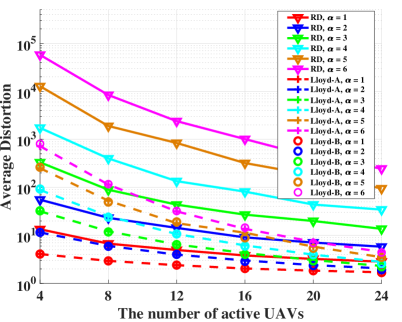
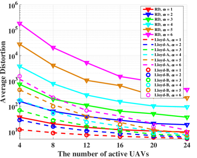
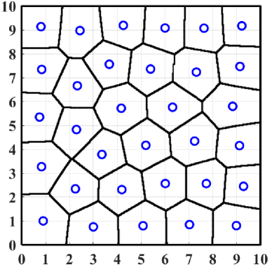
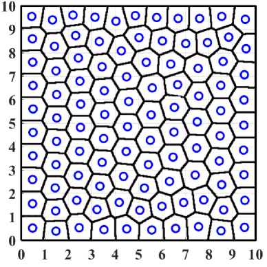
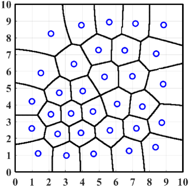
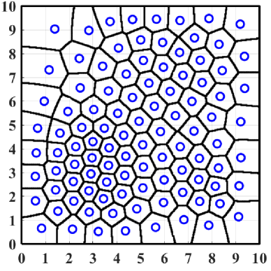
To evaluate the performance of the proposed algorithms, we compare them with the average distortion of $100$ random deployments (RDs). Figs. (4a) and (4b), show that the proposed algorithms outperform the random deployment on both uniform and non-uniform distributed target regions. From Fig. (4a), one can also find that the distortion achieved by Lloyd-A and Lloyd-B are very close, indicating that the optimality of the common height, as proved for the one-dimensional case in Section (III), might be extended to the two-dimensional case when the density function is uniform. However, one can find a non-negligible gap between Lloyd-A and Lloyd-B in Fig. (4b) where the density function is non-uniform. For instance, given $16$ UAVs and the path-loss exponent $\alpha=6$, Lloyd-A’s distortion is $40.17$ while Lloyd-B obtains a smaller distortion, $28.25$, by placing UAVs at different heights. Figs. (5a) and (5b) illustrate the UAV ground projections and their partitions on a uniform distributed square region. As the number of UAVs increases, the UAV partitions approximate hexagons which implies that the optimality of congruent partition (Theorem (1)) might be extended to uniformly distributed users for two-dimensional sources. However, the UAV projections in Figs. (6a) and (6b) show that congruent partition is no longer a necessary condition for the optimal quantizer when distribution is non-uniform.

(a)

(b)

Figure 5: The UAV projections on the ground with generalized Voronoi Diagrams where $\alpha=2$ and the source distribution is uniform. (a) 32 UAVs. (b) 100 UAVs.

(a)

(b)

Figure 6: The UAV projections on the ground with generalized Voronoi Diagrams where $\alpha=2$ and the source distribution is non-uniform. (a) 32 UAVs. (b) 100 UAVs.

V Conclusion

We studied quantizers with parameterized distortion measures for an application to UAV deployments. Instead of using the traditional mean distance square as the distortion, we introduce a distortion function which models the energy consumption of UAVs in dependence of their heights. We derived the unique parameter optimized quantizer – a uniform scalar quantizer with an optimal common parameter – for uniform source density in one-dimensional space. In addition, two Lloyd-like algorithms are designed to minimize the distortion in two-dimensional space. Numerical simulations demonstrate that the common weight property extends to two-dimensional space for a uniform density.

Appendix A Proof of Lemma (2)

To find the optimal $1-$level parameter quantizer $(x^{*},h^{*})$ for a uniform density $\lambda(\omega)=1/A$, we need to satisfy (27), i.e., for $\Omega=\mathcal{V}_{1}=\mathcal{V}_{1}^{*}=[0,A]$

$$0 =\int_{0}^{A}(x^{*}-\omega)\big{(}(x^{*}-\omega)^{2}+h^{*2}\big{)}^{\gamma-1}d\omega.$$ (33)

Substituting $x^{*}-\omega$ by $\omega$ we get

$$0 =\int_{x^{*}-A}^{x^{*}}\omega\big{(}\omega^{2}+h^{*2}\big{)}^{\gamma-1}d\omega.$$ (34)

Since the integral kernel is an odd function in $\omega$ and $x^{*}\in[0,A]$, it must hold

$$0=-\int_{0}^{x^{*}-A}\omega(\omega^{2}+h^{*2})^{\gamma-1}d\omega+\int_{0}^{x^{*}}\omega(\omega^{2}+h^{*2})^{\gamma-1}d\omega$$ (35)

by substituting $$\omega -\omega$$ by we get

$$\int_{0}^{A-x^{*}}\omega(\omega^{2}+h^{*2})^{\gamma-1}d\omega=\int_{0}^{x^{*}}\omega(\omega^{2}+h^{*2})^{\gamma-1}d\omega.$$ (36)

Hence for any choice of $h^{*}$ it must hold $x^{*}=A-x^{*}$, which is equivalent to $x^{*}=A/2$. To find the optimal parameter, we can just insert $x^{*}$ into the average distortion

$$\bar{D}(x^{*},h) =\frac{1}{A}\int_{0}^{A}\frac{(x^{*}-\omega)^{2}+h^{2})^{\gamma}}{h}d\omega=\frac{1}{A}\int_{0}^{A/2}\frac{(\omega^{2}+h^{2})^{\gamma}}{h}d\omega$$ (37)

where we substituted again and inserted $$x^{*}=A/2 \omega 2\omega/A h u=2h/A$$. By substituting with and with we get

$$=\int_{0}^{1}\frac{2}{A}\frac{((A\omega/2)^{2}+(Au/2)^{2})^{\gamma}}{u}d\omega=\left(\frac{A}{2}\right)^{2\gamma-1}\int_{0}^{1}f(\omega,u,\gamma)d\omega$$ (38)

where for each $\gamma\geq 1$ the integral kernel $f$ is a convex function in ${\mathbf{x}}=(\omega,u)$ over ${\mathbb{R}}_{+}^{2}$. Let us rewrite $f$ as

$$f(\omega,u,\gamma)=\frac{(\omega^{2}+u^{2})^{\gamma}}{u}=\frac{\left\|(\omega,u)\right\|_{2}^{2\gamma}}{u}.$$ (39)

Clearly, $\left\|{\mathbf{x}}\right\|_{2}$ is a convex and continuous function in ${\mathbf{x}}$ over ${\mathbb{R}}^{2}$ and since $(\cdot)^{2\gamma}$ with $2\gamma\geq 2$ is a strictly increasing continuous function, the concatenation $f({\mathbf{x}},\gamma)$ is a strict convex and continuous function over ${\mathbb{R}}_{+}^{2}$. Hence, for any ${\mathbf{x}}_{1},{\mathbf{x}}_{2}\in{\mathbb{R}}^{2}$ we have

$$\left\|\lambda{\mathbf{x}}_{1}+(1-\lambda){\mathbf{x}}_{2}\right\|_{2}^{2\gamma}<\lambda\left\|{\mathbf{x}}_{1}\right\|_{2}^{2\gamma}+(1-\lambda)\left\|{\mathbf{x}}_{2}\right\|_{2}^{2\gamma}$$ (40)

for all $\lambda\in(0,1)$. But then we have also for any $u_{1},u_{2}\in{\mathbb{R}}^{2}_{+}$ and $\omega\geq 0$

$$f(\lambda u_{1}+(1-\lambda)u_{2},\omega,\gamma)<\frac{\lambda\left\|(\omega,u_{1})\right\|_{2}^{2\gamma}+(1-\lambda)\left\|(\omega,u_{2})\right\|_{2}^{2\gamma}}{\lambda u_{1}+(1-\lambda)u_{2}}.$$ (41)

Considering the following inequality

$$\frac{1}{u_{1}}\!+\!\frac{1}{u_{2}} =\left(\frac{1}{u_{1}}\!+\!\frac{1}{u_{2}}\right)\frac{\lambda u_{1}\!+\!(1\!-\!\lambda)u_{2}}{\lambda u_{1}\!+\!(1\!-\!\lambda)u_{2}}=\frac{\left(\lambda\!+\!\frac{(1\!-\!\lambda)u_{2}}{u_{1}}\!+\!(1\!-\!\lambda)\!+\!\frac{\lambda u_{1}}{u_{2}}\right)}{\lambda u_{1}\!+\!(1\!-\!\lambda)u_{2}}>\frac{1}{\lambda u_{1}\!+\!(1\!-\!\lambda)u_{2}}$$

and (41), we will have

$$f(\lambda u_{1}+(1-\lambda)u_{2},\omega,\gamma)<\lambda f(u_{1},\omega,\gamma)+(1-\lambda)f(u_{2},\omega,\gamma)$$ (42)

for every $\lambda\in(0,1)$. Hence, the integral kernel is a strictly convex function for every $\omega\geq 0,\gamma\geq 1$, and since the infinite sum (integral) of convex functions is again a convex function, for $u>0$, we have shown convexity of $F(u,\gamma)$. Note, $f(u,\omega,\gamma)$ is continuous in ${\mathbb{R}}_{+}^{2}$ since it is a product of the continuous functions $\left\|(u,\omega)\right\|_{2}^{2\gamma}$ and $1/(u+0\cdot\omega)$, and so is $F(u,\gamma)$. Therefore, the only critical point of $F(\cdot,\gamma)$ will be the unique global minimizer

$$g(\gamma)=\arg\min_{u>0}F(u,\gamma),$$ (43)

which is defined by the vanishing of the first derivative:

$$F^{\prime}(u) \!=\!\int_{0}^{1}\!(\omega^{2}\!+\!u^{2})^{\gamma-1}\left((2\gamma\!-\!1)-\frac{\omega^{2}}{u^{2}}\right)d\omega\!=\!\frac{1}{u^{2}}\!\int_{0}^{1}(\omega^{2}\!+\!u^{2})^{\gamma-1}\left((2\gamma\!-\!1)u^{2}-\omega^{2}\right)d\omega.$$ (44)

Hence, $F^{\prime}(u)$ can only vanish if $u<1/\sqrt{2\gamma-1}$, which is an upper bound on $g(\gamma)$. The optimal parameter for minimizing the average distortion (37) is then

$$h^{*}=\frac{A}{2}g(\gamma)\quad\text{with}\quad\bar{D}(x^{*},h^{*})=\left(\frac{A}{2}\right)^{2\gamma-1}g(\gamma).$$ (45)

Analytical solutions for $F^{\prime}(u)=0$ are possible for integer valued $\gamma$. Let us set $0<x=u^{2}$ in (44), then for $\gamma\in{\mathbb{N}}$, the integrand in (44) will be a polynomial in $\omega$ of degree $2\gamma$ and in $x$ of degree $\gamma$. For $\gamma\in\{1,2,3\}$ the integrand will be

$$(\omega^{2}+x)^{0}(1x-\omega^{2}) =x-\omega^{2}$$ (46)

$$(\omega^{2}+x)^{1}(3x-\omega^{2}) =3x^{2}+2\omega^{2}x-\omega^{4}$$ (47)

$$(\omega^{2}+x)^{2}(5x-\omega^{2}) =5x^{3}+9\omega^{2}x^{2}+3\omega^{4}x-\omega^{6}$$ (48)

which yield with the definite integrals to

$$0 =\omega(x-\frac{\omega^{2}}{3})\Big{|}_{\omega=1}$$ (49)

$$0 =\omega(3x^{2}+\frac{2\omega^{2}x}{3}-\frac{\omega^{4}}{5})\Big{|}_{\omega=1}$$ (50)

$$0 =\omega(5x^{3}+3\omega^{2}x^{2}+\frac{3\omega^{4}x}{5}-\frac{\omega^{6}}{7})\Big{|}_{\omega=1}$$ (51)

Solving (49) for $x$ yields to the only feasible solution

$$x=\frac{1}{3}\quad\Rightarrow\quad g(1)=\frac{1}{\sqrt{3}}\approx 0.577.$$ (52)

The solutions of (50) are

$$x_{\pm}=-\frac{1}{9}\pm\sqrt{\frac{1}{81}+\frac{1}{15}}=\frac{\pm\sqrt{32/5}-1}{9}$$ (53)

Since only positive roots are allowed, we get as the only feasible solution

$$g(3)=\frac{\sqrt{\sqrt{32/5}-1}}{3}\approx 0.412.$$ (54)

Finally, the cubic equation (51) results in

$$5x^{3}+3x^{2}+\frac{3}{5}x-\frac{1}{7}=0$$ (55)

The solution of a cubic equation can be found in [Zwi03, 2.3.2] by calculating the discriminant

$$\Delta=q^{2}+4p^{3}\quad\text{with}\quad q=\frac{2b^{3}-9abc+27a^{2}d}{27a^{3}},p=\frac{3ac-b^{2}}{9a^{2}}$$ (56)

Let us identify $a=5,b=3,c=3/5$ and $d=-1/7$, then we get

$$q =\frac{6\cdot 9-9\cdot 9-27\cdot 5^{2}\cdot 1/7}{27\cdot 5^{3}}=-\frac{3}{3\cdot 5\cdot 25}-\frac{1}{5\cdot 7}=-\frac{32}{25\cdot 35}$$ (57)

$$\Delta =q^{2}+4\left(\frac{3\cdot 3-9}{9\cdot 5^{2}}\right)^{3}=q^{2}>0$$ (58)

which indicates only one real-valued root, given by

$$x=\alpha_{+}^{1/3}+\alpha_{-}^{1/3}-\frac{b}{3a}\quad\text{with}\quad\alpha_{\pm}=\frac{-q\pm\sqrt{\Delta}}{2}=\left\{0,\frac{32}{25\cdot 35}\right\}$$ (59)

which computes to

$$x=\left(\frac{32}{5^{3}\cdot 7}\right)^{1/3}-\frac{1}{5}=\frac{(\frac{32}{7})^{1/3}-1}{5}\Rightarrow g(5)=\sqrt{\frac{(\frac{32}{7})^{1/3}-1}{5}}\approx 0.363.$$ (60)

Appendix B Proof of Lemma (3)

Although, this statement seems to be trivial, it is not straight forward to show. We will use the quantization relaxation for the average distortion $\bar{D}$ in (9) to show that the $N-$level parameter optimized quantizer has strictly smaller distortion than the $(N-1)-$level optimized quantizer (10). We define, as in quantization theory, see for example [GN98], an $N-$level quantizer for $\Omega$, by a (disjoint) partition $\mathcal{R}=\{\mathcal{R}_{n}\}_{n=1}^{N}\subset\Omega$ of $\Omega$ and assign to each partition region $\mathcal{R}_{n}$ a quantization-parameter point $(\mathbf{q}_{n},h_{n})\in\Omega\times{\mathbb{R}}_{+}$. The assignment rule or quantization rule can be anything such that the regions are independent of the value of the quantization and parameter points. Minimizing over the quantizer, that is, over all partitions and possible quantization-parameter points will yield to the parameter optimized quantizer, which is by definition the optimal deployment which generate the generalized Voronoi regions as the optimal partition (tessellation). This holds for any density function $\lambda(\omega)$ and target area $\Omega$. To see this, let us start with any quantizer $(\mathbf{Q},{\mathbf{h}},\mathcal{R})$ for $\Omega$ yielding to the average distortion

$$\bar{D}(\mathbf{Q},{\mathbf{h}},\mathcal{R}) =\sum_{n=1}^{N}\int_{\mathcal{R}_{n}}D(\mathbf{q}_{n},h_{n},\omega)\lambda(\omega)d\omega\geq\sum_{n=1}^{N}\int_{\mathcal{R}_{n}}\left(\min_{m\in[N]}D(\mathbf{q}_{m},h_{n},\omega)\right)\lambda(\omega)d\omega$$

$$=\int_{\Omega}\min_{m\in[N]}D(\mathbf{q}_{m},h_{n},\omega)\lambda(\omega)d\omega=\sum_{n=1}^{N}\int_{\mathcal{V}_{n}(\mathbf{Q},{\mathbf{h}})}D(\mathbf{q}_{n},h_{n},\omega)\lambda(\omega)d\omega$$ (61)

where the first inequality is only achieved if for any $\omega\in\mathcal{R}_{n}$ we have chosen $(\mathbf{q}_{n},h_{n})$ to be the optimal quantization point with respect to $D$, or vice versa, if every $(\mathbf{q},h_{n})$ is optimal for every $\omega\in\mathcal{R}_{n}$, which is the definition of the generalized Voronoi region $\mathcal{V}(\mathbf{Q},{\mathbf{h}})$. Therefore, minimizing over all partitions gives equality, i.e.

$$\min_{\mathcal{R}}\bar{D}(\mathbf{Q},{\mathbf{h}},\mathcal{R})=\bar{D}(\mathbf{Q},{\mathbf{h}},\mathcal{V}(\mathbf{Q},{\mathbf{h}}))$$ (62)

for any $(\mathbf{Q},{\mathbf{h}})\in\Omega^{N}\times{\mathbb{R}}_{+}^{N}$. Hence, we have shown that the parameterized distortion quantizer optimization problem is equivalent to the locational-parameter optimization problem

$$\min_{\mathbf{Q}\in\Omega^{N},{\mathbf{h}}\in{\mathbb{R}}_{+}^{N}}\min_{\mathcal{R}\in\Omega^{N}}\bar{D}(\mathbf{Q},{\mathbf{h}},\mathcal{R})=\min_{\mathbf{Q}\in\Omega^{N},{\mathbf{h}}\in{\mathbb{R}}_{+}^{N}}\bar{D}(\mathbf{Q},{\mathbf{h}},\mathcal{V}(\mathbf{Q},{\mathbf{h}}))=\bar{D}(\mathbf{Q}^{*},{\mathbf{h}}^{*},\mathcal{V}^{*}).$$ (63)

We need to show that for the optimal $N-$level parameter-quantizer $(\mathbf{Q}^{*},{\mathbf{h}}^{*},\mathcal{V}^{*})$ with $\mathcal{V}^{*}=\mathcal{V}(\mathbf{Q}^{*},{\mathbf{h}}^{*})$, we have $\mu(\mathcal{V}_{n})>0$ for all $n\in[N]$. Let us first show that each region is indeed a closed interval, i.e., $\mathcal{V}_{n}^{*}=[b^{*}_{n-1},b^{*}_{n}]$ with $0\leq b^{*}_{n-1}\leq b^{*}_{n}\leq A$.

By the definition of the Möbius regions in Lemma (1), each dominance region is either a single interval (if it is a ball not contained in the target region or a halfspace) or two disjoint intervals (if its a ball contained in the target region), we can not have more than $K_{n}\leq 2N-2$ disjoint closed intervals for each Möbius (generalized Voronoi) region. Therefore, the $n$th optimal Möbius region is given as $\mathcal{V}^{*}_{n}=\bigcup_{k=1}^{K_{n}}v_{n,k}$, where $v_{n,k}=[a_{n,k-1},a_{n,k}]$ are intervals for some $0\leq a_{n,k-1}\leq a_{n,k}\leq A$.

Let us assume there are quantization points with disconnected regions, i.e. $K_{n}>1$ for $n\in\mathcal{I}_{d}$ and some $\mathcal{I}_{d}\subset[N]$. Then, we will re-arrange the partition $\mathcal{V}^{*}$ by concatenating the $K_{n}$ disconnected intervals $v_{n,k}$ to $\mathcal{R}_{n}=[b_{n-1},b_{n}]$ for $n\in\mathcal{I}_{d}$ and move the connected regions appropriatly such that for all $n\in[N]$ it holds $\mu(\mathcal{R}_{n})=\mu(\mathcal{V}^{*}_{n})=b_{n}-b_{n-1}$ and $b_{n-1}\leq b_{n}$, where we set $b_{0}=0$ and $b_{N}=A$. For the new concatenated regions, we move each $q_{n}^{*}$ to the center of the new arranged regions, i.e., $\tilde{q}_{n}=\frac{b_{n}+b_{n-1}}{2}$ for $n\in\mathcal{I}_{d}$. If for the connected regions $n\in[N]\setminus\mathcal{I}_{d}$, the quantization point $q^{*}_{n}$ is not centroidal, by placing it at the center of the corresponding closed interval, we will obtain a strictly smaller distortion by Lemma (2). Hence, for the optimal quantizer, the quantization points must be centroidal and we can assume $\tilde{q}_{n}=(b_{n}+b_{n-1})/2$ for all $n\in[N]$. In this rearrangement, we did not change the parameters $h_{n}^{*}$ at all. The rearranged partition $\mathcal{R}=\{\mathcal{R}_{n}\}$ and replaced quantization points $\tilde{\mathbf{q}}=(\tilde{q}_{1},\dots,\tilde{q}_{N})$ provide the average distortion

$$\bar{D}(\tilde{\mathbf{q}},{\mathbf{h}}^{*},\mathcal{R})=\sum_{n=1}^{N}\int_{b_{n-1}}^{b_{n}}\frac{((\tilde{q}_{n}\!-\!\omega)^{2}+h_{n}^{*2})^{\gamma}}{h_{n}^{*}}d\omega=2\sum_{n=1}^{N}\int_{0}^{\frac{b_{n}-b_{n-1}}{2}}\frac{(\omega^{2}+h_{n}^{*2})^{\gamma}}{h_{n}^{*}}d\omega$$ (64)

where we substituted $\omega$ by $\tilde{q}_{n}\!-\!\omega$. Since the function $(\omega^{2}+h_{n}^{*2})^{\gamma}$ is strictly monotone increasing in $\omega$ for each $\gamma>0$, for any $n\in\mathcal{I}_{d}$, we have

$$\bar{D}_{n}=\bar{D}(\tilde{q}_{n},h_{n}^{*},\mathcal{R}_{n})=2\int_{0}^{\frac{b_{n}-b_{n-1}}{2}}\frac{(\omega^{2}+h_{n}^{*2})^{\gamma}}{h_{n}^{*}}d\omega<\sum_{k=1}^{K_{n}}\int_{a_{n,k}-q_{n}^{*}}^{a_{n,k-1}-q_{n}^{*}}\frac{(\omega^{2}+h_{n}^{*2})^{\gamma}}{h_{n}^{*}}d\omega$$ (65)

since the non-zero gaps in $\bigcup_{k}[a_{n,k}-q_{n}^{*},a_{n,k-1}-q_{n}^{*}]$ will lead to larger $\omega$ in the RHS integral and therefore to a strictly larger average distortion. Therefore, the points $(\tilde{\mathbf{q}},{\mathbf{h}}^{*})$ with closed intervals $\{\mathcal{R}_{n}\}$ have a strictly smaller average distortion, which contradicts the assumption that $(\mathbf{q}^{*},{\mathbf{h}}^{*})$ is the parameter-optimized quantizer (11). Hence, $K_{n}=1$ for each $n\in[N]$ and every $\gamma\geq 1$. Moreover, the optimal quantization points must be centroids of the intervals, i.e. $x_{n}^{*}=(b_{n}^{*}+b^{*}_{n-1})/2$.

Now, we have to show that the optimal quantization regions $\mathcal{V}_{n}^{*}=\{[b^{*}_{n-1},b^{*}_{n}]\}_{n=1}^{N}$ are not points, i.e., it should hold $b^{*}_{n}>b^{*}_{n-1}$ for each $n\in[N]$. If $b^{*}_{n}=b^{*}_{n-1}$ for some $n$, then the $n$th average distortion $\bar{D}_{n}$ will be zero for this quantization point, since the integral is vanishing. But, then we only optimize over $N-1$ quantization points. So we only need to show that an additional quantization point strictly decreases the minimum average distortion. Hence, take any non-zero optimal quantization region $\mathcal{V}_{n}^{*}=[b^{*}_{n-1},b^{*}_{n}]$. We know by Lemma (2) that the optimal quantizer $q_{n}^{*}$ for some closed interval $\mathcal{V}_{n}^{*}$ must be centroidal for any parameter $h_{n}$. Hence, if we split $\mathcal{V}_{n}^{*}$ with $\mu_{n}^{*}=b^{*}_{n}-b^{*}_{n-1}$ by a half and put two quantizers $q_{n_{1}}$ and $q_{n_{2}}$ with the same parameter $h_{n}^{*}$ in the center, we will get by using (65)

$$\bar{D}_{n_{1}}\!+\!\bar{D}_{n_{2}} =\frac{1}{h_{n}^{*}}\left(\int_{b^{*}_{n-1}}^{b^{*}_{n-1}+\frac{\mu_{n}^{*}}{2}}((q_{n_{1}}-\omega)^{2}+h_{n}^{*2})^{\gamma}d\omega+\int_{b_{n-1}^{*}+\frac{\mu_{n}^{*}}{2}}^{b_{n}^{*}}((q_{n_{2}}-\omega)^{2}+h_{n}^{*2})^{\gamma}d\omega\right)$$

Substituting $$q_{n_{i}}-\omega \omega$$ by , we get

$$=\int_{-\frac{\mu_{n}^{*}}{4}}^{\frac{\mu_{n}^{*}}{4}}\frac{(\omega^{2}+h_{n}^{*2})^{\gamma}}{h_{n}^{*}}d\omega+\int_{-\frac{\mu_{n}^{*}}{4}}^{\frac{\mu_{n}^{*}}{4}}\frac{(\omega^{2}+h_{n}^{*2})^{\gamma}}{h_{n}^{*}}d\omega$$ (66)

$$=2\int_{0}^{\frac{\mu_{n}^{*}}{4}}\frac{(\omega^{2}+h_{n}^{*2})^{\gamma}}{h_{n}^{*}}d\omega+w\int_{0}^{\frac{\mu_{n}^{*}}{4}}\frac{(\omega^{2}+h_{n}^{*2})^{\gamma}}{h_{n}^{*}}d\omega$$ (67)

$$<2\!\int_{0}^{\frac{\mu_{n}^{*}}{4}}\frac{(\omega^{2}\!+\!h_{n}^{*2})^{\gamma}}{h_{n}^{*}}d\omega+2\!\int_{\frac{\mu_{n}^{*}}{4}}^{\frac{\mu_{n}^{*}}{2}}\frac{(\omega^{2}\!+\!h_{n}^{*2})^{\gamma}}{h_{n}^{*}}d\omega=2\!\int_{0}^{\frac{\mu_{n}^{*}}{2}}\frac{(\omega^{2}\!+\!h_{n}^{*2})^{\gamma}}{h_{n}^{*}}d\omega=\bar{D}_{n}.$$ (68)

Hence, the average distortion will strictly decrease if $\mu_{n}^{*}>0$. Therefore, the $N-$level parameter optimized quantizer will have quantization boundaries $b_{n}\!>\!b_{n\!-\!1}$ for $n\in[N]$.

Appendix C Proof of Theorem (1)

We know by Lemma (3) that the optimal quantization regions are closed non-vanishing intervals $\mathcal{V}_{n}^{*}=[b_{n-1}^{*},b_{n}^{*}]$ for some $b^{*}_{n-1}<b_{n}^{*}$ with quantization points

$$\mathbf{q}_{n}^{*}=x_{n}^{*}=\frac{b^{*}_{n}+b^{*}_{n-1}}{2}$$ (69)

for $n\in[N]$. Let us set $\mu_{n}^{*}=b_{n}^{*}-b_{n-1}^{*}$ for $n\in[N]$. By substituting $\frac{2(x_{n}^{*}-\omega)}{\mu_{n}}={\tilde{\omega}}$ and $h^{*}_{n}=\frac{u^{*}_{n}\mu_{n}^{*}}{2}$ in the average distortion, we get

$$\bar{D}(\mathbf{Q}^{*},{\mathbf{h}}^{*},\mathcal{V}^{*}) =\sum_{n=1}^{N}\int_{b_{n-1}^{*}}^{b_{n}^{*}}\frac{((x^{*}_{n}-\omega)^{2}+{h^{*}_{n}}^{2})^{\gamma}}{h^{*}_{n}}\frac{d\omega}{A}=\sum_{n=1}^{N}\int_{1}^{-1}-\frac{(\mu_{n}^{*2}{\tilde{\omega}}^{2}/4+u_{n}^{*2}\mu_{n}^{*2}/4)^{\gamma}}{u_{n}^{*}\mu_{n}^{*}/2}\frac{\mu_{n}}{2A}d{\tilde{\omega}}$$

$$=\frac{1}{2^{2\gamma-1}A}\sum_{n=1}^{N}\mu_{n}^{*2\gamma}\cdot\int_{0}^{1}\frac{(\omega^{2}+u^{*2}_{n})^{\gamma}}{u^{*}_{n}}d\omega$$ (70)

where we used (69) to get for the integral boundaries $2(x^{*}_{n}-b_{n-1}^{*})/\mu_{n}^{*}=1=-2(x^{*}_{n}-b_{n}^{*})/\mu^{*}_{n}$. We do not know the value of $u^{*}_{n}$ and $\mu_{n}^{*}$ but we know that $\mu_{n}^{*}>0$ and $\sum_{n=1}^{N}\mu_{n}^{*}=A$ by Lemma (3). Furthermore, (70) is the minimum over all such $\mu_{n}>0$ and $u_{n}>0$. Hence, it must hold

$$\bar{D}(\mathbf{Q}^{*},{\mathbf{h}}^{*},\mathcal{V}^{*})=\frac{1}{2^{2\gamma-1}A}\min_{u_{n}>0}\min_{\begin{subarray}{c}\mu_{n}>0\\ A\!=\!\sum_{n\!=\!1}^{N}\mu_{n}\end{subarray}}\sum_{n=1}^{N}\mu_{n}^{2\gamma}\cdot\left(\int_{0}^{1}\frac{(\omega^{2}+u^{2}_{n})^{\gamma}}{u_{n}}d\omega\right)=\frac{g(\gamma)}{2^{2\gamma-1}A}\min_{\begin{subarray}{c}\mu_{n}>0\\ A\!=\!\sum_{n\!=\!1}^{N}\mu_{n}\end{subarray}}\sum_{n=1}^{N}\mu_{n}^{2\gamma}$$

where in the last equality we used Lemma (2). By the Hölder inequality we get for $p=2\gamma,q=2\gamma/(2\gamma-1)$

$$\sum_{n=1}^{N}\mu_{n}^{2\gamma}=\sum_{n=1}^{N}\mu_{n}^{p}=\sum_{n=1}^{N}\mu_{n}^{p}\cdot\Big{(}\sum_{n=1}^{N}(1/N)^{q}\Big{)}^{p/q}\cdot N\geq\Big{(}\sum_{n=1}^{N}\frac{\mu_{n}}{N}\Big{)}^{p}\cdot N=\left(\frac{A}{N}\right)^{2\gamma}N$$

where the equality is achieved if and only if $\mu_{n}^{*}=A/N$. Hence, the optimal parameter-quantizer is the uniform scalar quantizer $x_{n}^{*}=(2n-1)A/2N$ with identical parameters $h^{*}=(A/2N)g(\gamma)$ resulting in the minimum average distortion (31).

Let us note here, that for identical parameters, the Möbius regions are closed intervals and reduce to Euclidean Voronoi regions by Lemma (1), for which the optimal tessellation is known to be the uniform scalar quantizer, see for example [GN98].

References