Learning and Interpreting Multi-Multi-Instance Learning Networks

Abstract

We introduce an extension of the multi-instance learning problem where examples are organized as nested bags of instances (e.g., a document could be represented as a bag of sentences, which in turn are bags of words). This framework can be useful in various scenarios, such as text and image classification, but also supervised learning over graphs. As a further advantage, multi-multi instance learning enables a particular way of interpreting predictions and the decision function. Our approach is based on a special neural network layer, called bag-layer, whose units aggregate bags of inputs of arbitrary size. We prove theoretically that the associated class of functions contains all Boolean functions over sets of sets of instances and we provide empirical evidence that functions of this kind can be actually learned on semi-synthetic datasets. We finally present experiments on text classification, on citation graphs, and social graph data, which show that our model obtains competitive results with respect to accuracy when compared to other approaches such as convolutional networks on graphs, while at the same time it supports a general approach to interpret the learnt model, as well as explain individual predictions.

Keywords: Multi-multi instance learning, relational learning, deep learning

1 Introduction

Relational learning takes several different forms ranging from purely symbolic (logical) representations, to a wide collection of statistical approaches (De Raedt et al., 2008a) based on tools such as probabilistic graphical models (Jaeger, 1997; De Raedt et al., 2008b; Richardson and Domingos, 2006; Getoor and Taskar, 2007), kernel machines (Landwehr et al., 2010), and neural networks (Frasconi et al., 1998; Scarselli et al., 2009; Niepert et al., 2016).

Multi-instance learning (MIL) is perhaps the simplest form of relational learning where data consists of labeled bags of instances. Introduced in (Dietterich et al., 1997), MIL has attracted the attention of several researchers during the last two decades and has been successfully applied to problems such as image and scene classification (Maron and Ratan, 1998; Zha et al., 2008; Zhou et al., 2012), image annotation (Yang et al., 2006), image retrieval (Yang and Lozano-Perez, 2000; Rahmani et al., 2005), Web mining (Zhou et al., 2005), text categorization (Zhou et al., 2012) and diagnostic medical imaging (Hou et al., 2015; Yan et al., 2016). In classic MIL, labels are binary and bags are positive iff they contain at least one positive instance (existential semantics). For example, a visual scene with animals could be labeled as positive iff it contains at least one tiger. Various families of algorithms have been proposed for MIL, including axis parallel rectangles (Dietterich et al., 1997), diverse density (Maron and Lozano-Pérez, 1998), nearest neighbors (Wang and Zucker, 2000), neural networks (Ramon and De Raedt, 2000), and variants of support vector machines (Andrews et al., 2002). Several other formulations of MIL are possible, see e.g. (Foulds and Frank, 2010) and under the mildest assumptions MIL and supervised learning on sets, i.e. the problem also formulated in previous works such as (Kondor and Jebara, 2003; Vinyals et al., 2016; Zaheer et al., 2017), essentially come together.

In this paper, we extend the MIL setting by considering examples consisting of labeled nested bags of instances. Labels are observed for top-level bags, while instances and lower level bags have associated latent labels. For example, a potential offside situation in a soccer match can be represented by a bag of images showing the scene from different camera perspectives. Each image, in turn, can be interpreted as a bag of players with latent labels for their team membership and/or position on the field. We call this setting multi-multi-instance learning (MMIL), referring specifically to the case of bags-of-bags. In our framework, we also relax the classic MIL assumption of binary instance labels, allowing categorical labels lying in a generic alphabet. This is important since MMIL with binary labels under the existential semantics would reduce to classic MIL after flattening the bag-of-bags.

Our solution to the MMIL problem is based on neural networks with a special layer called bag-layer (Tibo et al., 2017), which fundamentally relies on weight sharing like other neural network architectures such as convolutional networks (LeCun et al., 1989), graph convolutional networks (Kipf and Welling, 2016; Gilmer et al., 2017) and essentially coincides with the invariant model used in DeepSets (Zaheer et al., 2017). Unlike previous neural network approaches to MIL learning (Ramon and De Raedt, 2000), where predicted instance labels are aggregated by (a soft version of) the maximum operator, bag-layers aggregate internal representations of instances (or bags of instances) and can be naturally intermixed with other layers commonly used in deep learning. Bag-layers can be in fact interpreted as a generalization of convolutional layers followed by pooling, as commonly used in deep learning.

The MMIL framework can be immediately applied to solve problems where examples are naturally described as bags-of-bags. For example, a text document can be described as a bag of sentences, where in turn each sentence is a bag of words. The range of possible applications of the framework is however larger. In fact, every structured data object can be recursively decomposed into parts, a strategy that has been widely applied in the context of graph kernels (see e.g., (Haussler, 1999; Gärtner et al., 2004; Passerini et al., 2006; Shervashidze et al., 2009; Costa and De Grave, 2010; Orsini et al., 2015)). Hence, MMIL is also applicable to supervised graph classification. Experiments on bibliographical and social network datasets confirm the practical viability of MMIL for these forms of relational learning.

As a further advantage, multi-multi instance learning enables a particular way of interpreting the models by reconstructing instance and sub-bag latent variables. This allows to explain the prediction for a particular data point, and to describe the structure of the decision function in terms of symbolic rules. Suppose we could recover the latent labels associated with instances or inner bags. These labels would provide useful additional information about the data since we could group instances (or inner bags) that share the same latent label and attach some semantics to these groups by inspection. For example, in the case of textual data, grouping words or sentences with the same latent label effectively discovers topics and the decision of a MMIL text document classifier can be interpreted in terms of the discovered topics. In practice, even if we cannot recover the true latent labels, we may still cluster the patterns of hidden units activations in the bag-layers and use the cluster indices as surrogates of the latent labels.

This paper is an extended version of (Tibo et al., 2017), where the MMIL problem was first introduced and solved with networks of bag layers. The main extensions contained in this paper are a general strategy for interpreting MMIL networks via clustering and logical rules, and a much extended range of experiments on real-world data. The paper is organized as follows. In Section 2 we formally introduce the MMIL setting. In Section 2.3 we introduce bag layers and the resulting neural network architecture for MMIL, and derive a theoretical expressivity result. Section 3 relates MMIL to standard graph learning problems. Section 4 describes our approach to interpreting MMIL networks by extracting logical rules from trained networks of bag-layers. In Section 5 we discuss some related works. in Section 6 we report experimental results on five different types of real-world datasets. Finally we draw some conclusions in Section 7.

2 Framework

2.1 Traditional Multi-Instance Learning

In the standard multi-instance learning (MIL) setting, data consists of labeled bags of instances. In the following, $\mathcal{X}$ denotes the instance space (it can be any set), $\mathcal{Y}$ the bag label space for the observed labels of example bags, and $\mathcal{Y}^{\mathrm{inst}}$ the instance label space for the unobserved (latent) instance labels. For any set $A$, ${M}(A)$ denotes the set of all multisets of $A$. An example in MIL is a pair $(x,y)\in{M}(\mathcal{X})\times\mathcal{Y}$, which we interpret as the observed part of an instance-labeled example $(x^{\mathrm{labeled}},y)\in{M}(\mathcal{X}\times\mathcal{Y}^{\mathrm{inst}})\times\mathcal{Y}$. $x=\{x_{1},\dots,x_{n}\}$ is thus a multiset of instances, and $x^{\mathrm{labeled}}=\{(x_{1},y_{1}),\dots,(x_{n},y_{n})\}$ a multiset of labeled instances.

Examples are drawn from a fixed and unknown distribution $p(x^{\mathrm{labeled}},y)$. Furthermore, it is typically assumed that the label of an example is conditionally independent of the individual instances given their labels, i.e. $p(y|(x_{1},y_{1}),\dots,(x_{n},y_{n}))=p(y|y_{1},\dots,y_{n})$ In the classic setting, introduced in (Dietterich, 2000) and used in several subsequent works (Maron and Lozano-Pérez, 1998; Wang and Zucker, 2000; Andrews et al., 2002), the focus is on binary classification ($\mathcal{Y}^{\mathrm{inst}}=\mathcal{Y}=\{0,1\}$) and it is postulated that $y=\mathds{1}\!\left\{0<\sum_{j}y_{j}\right\}$, (i.e., an example is positive iff at least one of its instances is positive). More complex assumptions are possible and thoroughly reviewed in (Foulds and Frank, 2010). Supervised learning in this setting can be formulated in two ways: (1) learn a function $F:{M}(\mathcal{X})\mapsto\mathcal{Y}$ that classifies whole examples, or (2) learn a function $f:\mathcal{X}\mapsto\mathcal{Y}^{\mathrm{inst}}$ that classifies instances and then use some aggregation function defined on the multiset of predicted instance labels to obtain the example label.

2.2 Multi-Multi-Instance Learning

In multi-multi-instance learning (MMIL), data consists of labeled nested bags of instances. When the level of nesting is two, an example is a labeled bag-of-bags $(x,y)\in{M}({M}(\mathcal{X}))\times\mathcal{Y}$ drawn from a distribution $p(x,y)$. Deeper levels of nesting, leading to multi^K-instance learning are conceptually easy to introduce but we avoid them in the paper to keep our notation simple. We will also informally use the expression “bag-of-bags” to describe structures with two or more levels of nesting. In the MMIL setting, we call the elements of ${M}({M}(\mathcal{X}))$ and ${M}(\mathcal{X})$ top-bags and sub-bags, respectively.

Now postulating unobserved labels for both the instances and the sub-bags, we interpret examples $(x,y)$ as the observed part of fully labeled data points $(x^{\mathrm{labeled}},y)\in{M}({M}(\mathcal{X}\times\mathcal{Y}^{\mathrm{inst}})\times\mathcal{Y}^{\mathrm{sub}})\times\mathcal{Y}$, where $\mathcal{Y}^{\mathrm{sub}}$ is the space of sub-bag labels. Fully labeled data points are drawn from a distribution $p(x^{\mathrm{labeled}},y)$.

As in MIL, we make some conditional independence assumptions. Specifically, we assume that instance and sub-bag labels only depend on properties of the respective instances or sub-bags, and not on other elements in the nested multiset structure $x^{\mathrm{labeled}}$ (thus excluding models for contagion or homophily, where, e.g., a specific label for an instance could become more likely, if many other instances contained in the same sub-bag also have that label). Furthermore, we assume that labels of sub-bags and top-bags only depend on the labels of their constituent elements. Thus, for $y_{j}\in\mathcal{Y}^{\mathrm{sub}}$, and a bag of labeled instances $S^{\mathrm{labeled}}=\{(x_{{j},{1}},y_{{j},{1}}),\ldots,(x_{{j},{n_{j}}},y_{{j},{n_{j}}})\}$ we have:

$$p(y_{j}|S^{\mathrm{labeled}})=p(y_{j}|y_{{j},{1}},\dots y_{{j},{n_{j}}}).$$ (1)

Similarly for the probability distribution of top-bag labels given the constituent labeled sub-bags.

Example 2.1.

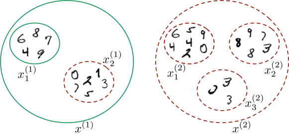
In this example we consider bags-of-bags of handwritten digits (as in the MNIST dataset). Each instance (a digit) has attached its own latent class label in $\{0,\dots,9\}$ whereas sub-bag (latent) and top-bag labels (observed) are binary. In particular, a sub-bag is positive iff it contains an instance of class 7 and does not contain an instance of class 3. A top-bag is positive iff it contains at least one positive sub-bag. Figure 1 shows a positive and a negative example.

Figure 1: A positive (left) and a negative (right) top-bag for Example 2.1. Solid green lines represent positive (sub-) bags while dashed red lines represent negative (sub-) bags.

Example 2.2.

A top-bag can consist of a set of images showing a potential offside situation in soccer from different camera perspectives. The label of the bag corresponds to the referee decision $\mathcal{Y}\in\{\mbox{offside},\mbox{not offside}\}$. Each individual image can either settle the offside question one way or another, or be inconclusive. Thus, there are (latent) image labels $\mathcal{Y}^{\mathrm{sub}}\in\{\mbox{offside},\mbox{not offside},\mbox{inconclusive}\}$. Since no offside should be called when in doubt, the top-bag is labeled as ‘not offside’ if and only if it either contains at least one image labeled ‘not offside’, or all the images are labeled ‘inconclusive’. Images, in turn, can be seen as bags of player instances that have a label $\mathcal{Y}^{\mathrm{inst}}\in\{\mbox{behind},\mbox{in front},\mbox{inconclusive}\}$ according to their relative position with respect to the potentially offside player of the other team. An image then is labeled ‘offside’ if all the players in the image are labeled ‘behind’; it is labeled ‘not offside’ if it contains at least one player labeled ‘in front’, and is labeled ‘inconclusive’ if it only contains players labeled ‘inconclusive’ or ‘behind’.

Example 2.3.

In text categorization, the bag-of-word representation is often used to feed documents to classifiers. Each instance in this case consists of the indicator vector of words in the document (or a weighted variant such as TF-IDF). The MIL approach has been applied in some cases (Andrews et al., 2002) where instances consist of chunks of consecutive words and each instance is an indicator vector. A bag-of-bags representation could instead describe a document as a bag of sentences, and each sentence as a bag of word vectors (constructed for example using Word2vec or GloVe).

2.3 A Network Architecture for MMIL

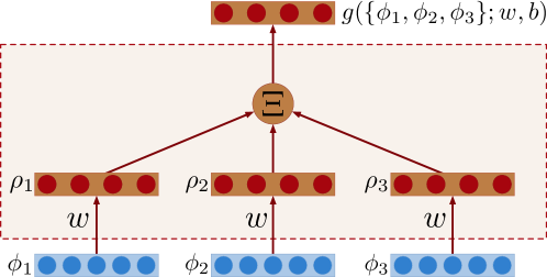
We model the conditional distribution $p(y|x)$ with a neural network architecture that handles bags-of-bags of variable sizes by aggregating intermediate internal representations. For this purpose, we define a bag-layer as follows:

• the input is a bag of $m$-dimensional vectors. $\{\phi_{1},\dots,\phi_{n}\}$

• First, $k$-dimensional representations are computed as

  $$\rho_{i}=\alpha\left(w\phi_{i}+b\right)$$ (2)

  using a weight matrix $w\in\mathds{R}^{k\times m}$, a bias vector $b\in\mathds{R}^{k}$ (both tunable parameters), and an activation function $\alpha$ (such as ReLU, tanh, or linear).

• The output is

  $$g(\{\phi_{1},\dots,\phi_{n}\};w,b)=\operatorname*{\Xi}_{i=1}^{n}\rho_{i}$$ (3)

  where $\operatorname*{\Xi}$ is element-wise aggregation operator (such as max or average). Both $w$ and $b$ are tunable parameters.

Note that Equation 3 works with bags of arbitrary cardinality. A bag-layer is illustrated in Figure 2.

Figure 2: A bag-layer receiving a bag of cardinality $n=3$. In this example $k=4$ and $m=5$.

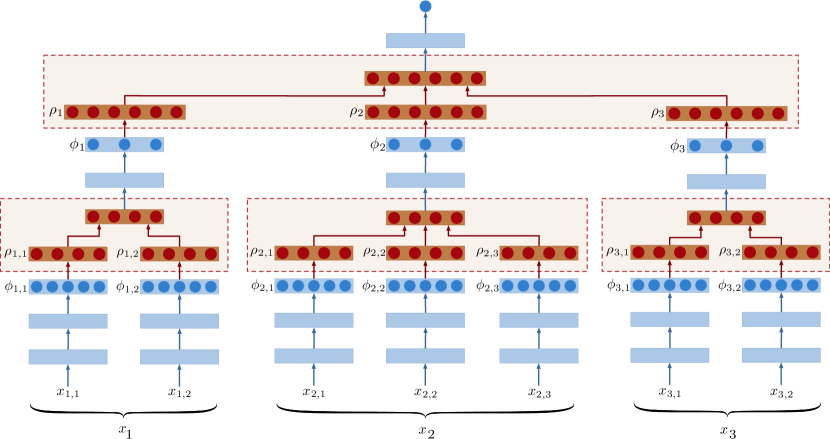
Networks with a single bag-layer can process bags of instances (as in the standard MIL setting). To solve the MMIL problem, two bag-layers are required. The bottom bag-layer aggregates over internal representations of instances; the top bag-layer aggregates over internal representations of sub-bags, yielding a representation for the entire top-bag. In this case, the representation of each sub-bag $x_{j}=\{x_{{j},{1}},\dots,x_{{j},{n_{j}}}\}$ would be obtained as

$$\phi_{j}=g(\{x_{{j},{1}},\dots,x_{{j},{n_{j}}}\};w^{\mathrm{inst}},b^{\mathrm{inst}})\ \ j=1,\dots,n$$ (4)

and the representation of a top-bag $x=\{x_{1},\dots,x_{n}\}$ would be obtained as

$$\phi=g(\{\phi_{1},\dots,\phi_{n}\};w^{\mathrm{sub}},b^{\mathrm{sub}})$$ (5)

where $(w^{\mathrm{inst}},b^{\mathrm{inst}})$ and $(w^{\mathrm{sub}},b^{\mathrm{sub}})$ denote the parameters used to construct sub-bag and top-bag representations. Multiple bag-layers with different aggregation functions can be also be used in parallel, and bag-layers can be intermixed with standard neural network layers, thereby forming networks of arbitrary depth. An illustration of a possible overall architecture involving two bag-layers is shown in Figure 3.

Figure 3: Network for multi-multi instance learning applied to the bag-of-bags $\{\{x_{1,1},x_{1,2}\},\{x_{2,1},x_{2,2},x_{2,2}\},\{x_{3,1},x_{3,2}\}\}$. Bag-layers are depicted in red with dashed borders. Blue boxes are standard (e.g., dense) neural network layers. Parameters in each of the seven bottom vertical columns are shared, and so are the parameters in the middle three columns.

It is shown in (Tibo et al., 2017) that networks with two bag layers with max aggregation can solve all MMIL problems that satisfy the restrictions if being deterministic (essentially saying that the conditional probability distributions (1) become deterministic functions) and non-counting (the multiplicities of elements in the bags do not matter).

3 MMIL for Graph Learning

The MMIL perspective can also be used to derive algorithms suitable for supervised learning over graphs, i.e., tasks such as graph classification, node classification, and edge prediction. In all these cases, one first needs to construct a representation for the object of interest (a whole graph, a node, a pair of nodes) and then apply a classifier. A suitable representation can be obtained in our framework by first forming a bag-of-bags associated with the object of interest (a graph, a node, or an edge) and then feeding it to a network with bag-layers. In order to construct bags-of-bags, we follow the classic $R$-decomposition strategy introduced by Haussler (1999). In the present context, it simply requires us to introduce a relation $R(A,a)$ which holds true if $a$ is a “part” of $A$ and to form $R^{-1}(A)=\{a:R(A,a)\}$, the bag of all parts of $A$. Parts can in turn be decomposed in a similar fashion, yielding bags-of-bags. In the following, we focus on undirected graphs $G=(V,E)$ where $V$ is the set of nodes and $E=\{\{u,v\}:u,v\in V\}$ is the set of edges. We also assume that a labeling function $\xi:V\mapsto\mathcal{X}$ attaches attributes to vertices. Variants with directed graphs or labeled edges are straightforward and omitted here in the interest of brevity.

Graph classification.

A simple solution is to define the part-of relation $R(G,g)$ between graphs to hold true iff $g$ is a subgraph of $G$ and to introduce a second part-of relation $S(g,v)$ that holds true iff $v$ is a node in $g$. The bag-of-bags associated with $G$ is then constructed as $x=\{\{\xi(v):v\in S^{-1}(g)\}:g\in R^{-1}(G)\}$. In general, considering all subgraphs is not practical but suitable feasible choices for $R$ can be derived borrowing approaches already introduced in the graph kernel literature, for example decomposing $G$ into cycles and trees (Horváth et al., 2004), or into neighbors or neighbor pairs (Costa and De Grave, 2010) (some of these choices may require three levels of bag nesting, e.g., for grouping cycles and trees separately).

Node classification.

In some domains, the node labeling function itself is bag-valued. For example in a citation network, $\xi(v)$ could be the bag of words in the abstract of the paper associated with node $v$. A bag-of-bags in this case may be formed by considering a paper $v$ together all papers in its neighborhood $N(v)$ (i.e., its cites and citations): $x^{(v)}=\{\xi(u),u\in\{v\}\cup N(v)\}$. A slightly more rich description with three layers of nesting could be used to set apart a node and its neighborhood: $x^{(v)}=\{\{\xi(v)\},\{\xi(u),u\in N(v)\}\}$.

4 Interpreting Networks of Bag-Layers

Interpreting the predictions in the supervised learning setting amounts to provide a human understandable explanation of the prediction. Transparent techniques such as rules or trees retain much of the symbolic structure of the data and are well suited in this respect. On the contrary, predictions produced by methods based on numerical representations are often opaque, i.e., difficult to explain to humans. In particular, representations in neural networks are highly distributed, making it hard to disentangle a clear semantic interpretation of any specific hidden unit. Although many works exist that attempt to interpret neural networks, they mostly focus on specific application domains such as vision (Lapuschkin et al., 2016; Samek et al., 2016).

The MMIL settings offers some advantages in this respect. Indeed, if instance or sub-bag labels were observed, they would provide more information about bag-of-bags than mere predictions. To clarify our vision, MIL approaches like mi-SVM and MI-SVM in (Andrews et al., 2002) are not equally interpretable: the former is more interpretable than the latter since it also provides individual instance labels rather than simply providing a prediction about the whole bag. These standard MIL approaches make two assumptions: first all labels are binary, second the relationship between the instance labels and the bag label is predefined to be the existential quantifier. The MMIL model relaxes these assumptions by allowing labels in an a-priori unknown categorical alphabet, and by allowing more complex mappings between bags of instance labels and sub-bag labels. We follow the standard MIL approaches in that our interpretation approach is also based on the assumption of a deterministic mapping from component to bag labels, i.e., 0,1-valued probabilities in (1).

The idea we propose in the following consists of two major components. First, given MMIL data and a MMIL network, we infer label sets $\mathcal{C}^{\mathrm{inst}},\mathcal{C}^{\mathrm{sub}}$, labeling functions for instances and sub-bags, and sets of rules for the mapping from instance to sub-bag labels, and sub-bag to top-bag labels. This component is purely algorithmic and described in Section 4.1. Second, in order to support interpretation, semantic explanations of the constructed labels and inferred rules are provided. This component is hightly domain and data-depend. Several general solution strategies are described in Section 4.2.

4.1 Learning Symbolic Rules

For ease of exposition, we first describe the construction of synthetic labels and the learning of classification rules as two separate procedures. In the final algorithm these two procedures are interleaved (cf. Algorithms 1, 2 3).

Synthetic Label Construction.

We construct sets $\mathcal{C}^{\mathrm{inst}},\mathcal{C}^{\mathrm{sub}}$ as clusters of internal instance and sub-bag representations. Let $F$ be a MMIL network trained on labeled top-bag data $\{(x^{(i)},y^{(i)}),i=1,\dots,m\}$. Let $k^{\mathrm{inst}},k^{\mathrm{sub}}$ be target cardinalities for $\mathcal{C}^{\mathrm{inst}}$ and $\mathcal{C}^{\mathrm{sub}}$, respectively.

The inputs $\{x^{(i)},i=1,\dots,m\}$ generate multi-sets of sub-bag and instance representations computed by the bag layers of $F$:

$$S=\{\rho^{(i)}_{j}\mid i=1,\dots,m,j=1,\dots,n^{(i)}\}.$$ (6)

$$I=\{\rho^{(i)}_{j,\ell}\mid i=1,\dots,m,j=1,\dots,n^{(i)},\ell=1,\dots,n_{j}^{(i)}\}$$ (7)

where the $\rho^{(i)}_{j}$ and $\rho^{(i)}_{j,\ell}$ are the representations according to (2) (cf. Figure 3). We cluster (separately) the sets $I,S$, setting the target number of clusters to $k^{\mathrm{inst}}$ and $k^{\mathrm{sub}}$, respectively. Each resulting cluster is associated with a synthetic cluster identifier $u_{i}$, respectively $v_{i}$, so that $\mathcal{C}^{\mathrm{inst}}:=\{u_{1},\ldots,u_{k^{\mathrm{inst}}}\}$ and $\mathcal{C}^{\mathrm{sub}}:=\{v_{1},\ldots,v_{k^{\mathrm{sub}}}\}$. Any instance $x_{{j},{\ell}}$ and sub-bag $x_{j}$ in an example $x$ (either one of the training examples $x^{(i)}$, or a new test example) is then associated with the identifier of the cluster whose centroid is closest to the representation $\rho_{j,\ell}$, respectively $\rho_{j}$ computed by $F$ on $x$. We denote the resulting labeling with cluster identifiers by $y_{{j},{\ell}}^{(i)}\in\mathcal{C}^{\mathrm{inst}}$ and $y_{j}^{(i)}\in\mathcal{C}^{\mathrm{sub}}$.

We use K-means clustering as the underlying clustering method. While other clustering methods could be considered, it is important that the clustering method also provides a function that maps new examples to one of the constructed clusters.

Learning rules.

We next describe how we construct symbolic rules that approximate the actual (potentially noisy) relationships between cluster identifiers in the MMIL network.

Let us denote a bag of cluster identifiers as $\{y_{\ell}:c_{\ell}\mid\ell=1,\dots,|\mathcal{Y}|\}$, where $c_{\ell}$ is the multiplicity of $y_{\ell}$. An attribute-value representation of the bag can be immediately obtained in the form of a frequency vector $(f_{c_{1}},\ldots,f_{c_{|\mathcal{Y}|}})$, where $f_{c_{\ell}}=c_{\ell}/\sum_{p=1}^{|\mathcal{Y}|}c_{p}$ is the frequency of identifier $\ell$ in the bag. Alternatively, we can also use a $0/1$-valued occurrence vector $(o_{c_{1}},\ldots,o_{c_{|\mathcal{Y}|}})$ with $o_{c_{l}}=\mathds{1}\!\left\{c_{l}>0\right\}$. Jointly with the example label $y$, this attribute-value representation provides a supervised example that is now described at a compact symbolic level. Examples of this kind are well suited for transparent and interpretable classifiers that can naturally operate at the symbolic level. Any rule-based learner could be applied here and in the following we will use decision trees because of their simplicity and low bias.

In the two level MMIL case, we learn in this way functions $s,t$ mapping multisets of instance cluster identifiers to sub-bag cluster identifiers, and multisets of sub-bag cluster identifiers to top-bag labels, respectively. In the second case, our target labels are the predicted labels of the original MMIL network, not the actual labels of the training examples. Thus, we aim to construct rules that best approximate the MMIL model, not rules that provide the highest accuracy themselves.

Let $r(x_{{j},{\ell}}):=y_{{j},{\ell}}$ be the instance labeling function defined for all $x_{{j},{\ell}}\in\mathcal{X}$. Together with the learned functions $s,t$ we obtain a complete classification model for a top-bag based on the input features of its instances: $\hat{F}(x)\doteq t(s(r(x)))$. We refer to the accuracy of this model with regard to the predictions of the original MMIL model as its fidelity, defined as

$$\mathrm{Fidelity}=\frac{1}{|\mathcal{D}|}\sum_{(x,y)\in\mathcal{D}}\mathds{1}\!\left\{F(x)=\hat{F}(x)\right\}.$$

We use fidelity on a validation set as the criterion to select the cardinalities for $\mathcal{C}^{\mathrm{sub}}$ and $\mathcal{C}^{\mathrm{inst}}$ by performing a grid search over $k^{\mathrm{sub}},k^{\mathrm{inst}}$ value combinations. In Algorithms 1, 2,  3 we reported the pseudo-codes for learning the best symbolic rules for a MMIL network $F$. In particular Algorithm 1 computes an explainer, an object consisting of cluster centroids and a decision tree, for interpreting a single level of $F$. Algorithm 2 calculates the fidelity score, and Algorithm 3 searches the best explainer for $F$. For the sake of simplicity we condensed the pseudo-codes by exploiting the following subroutines:

• Flatten($S$) is a function which takes as input a set of multi-sets and return a set containing all the elements of each multi-set of $S$;

• KMeans($T$, $k$) is the KMeans algorithm which takes as input a set of vectors $T$ and $k$ clusters and returns the $k$ $centroids$;

• Assign-Labels($S$, $centroids$) is a function that takes as input a set of multi-sets $S$ and returns a set of multi-sets $labels$. $labels$ has the same structure of $S$ and each instance is replaced by its cluster index with respect to the $centroids$;

• Frequencies($labels$) is a function which takes as input a set of multi-sets $S$ of cluster index and returns for each multi-set a vectors containing the frequencies of each cluster index within the muti-set;

• Intermediate-Representations($F$, $X$) takes as input a MMIL network $F$ and a set of top-bags $X$ and return the multi-sets of intermediate representations for sub-bags and instances as described in Equations 6 and 7, respectively.

4.2 Explaining Rules and Predictions

The functions $r$, $s$, $t$ provide a complete symbolic approximation $\hat{F}$ of the given MMIL model $F$. Being expressed in terms of a (small number of) categorical symbols and simple classification rules, this approximation is more amenable to human interpretation than the original $F$. However, the interpretability of $\hat{F}$ sill hinges on the interpretability of its constituents, notably the semantic interpretability of the cluster identifiers. There is no general algorithmic solution to provide such semantic interpretations, but a range of possible (standard) strategies that we briefly mention here, and whose use in our particular context is illustrated in our experiments:

• Direct visualization: in the case where the instances forming a cluster are given by points in low-dimensional Euclidean space, whole clusters can be plotted directly. Examples of this case will be found in Sections 6.5 and 6.6.

• Cluster representatives: often clusters are described in terms of a small number of most representative elements. For example, in the case of textual data, this was suggested in the area of topic modelling (Blei et al., 2003; Griffiths and Steyvers, 2004). We follow a similar approach in Section 6.2.

• Ground truth labels: in some cases the cluster elements may be equipped with some true, latent label. In such cases we can alternatively characterize clusters in terms of their association with these actual labels. An example of this can be found in Section 6.1.

$\hat{F}$ in conjunction with an interpretation of the cluster identifiers constitutes a global (approximate) explanation of the model $F$. This global explanation leads to example-specific explanations of individual predictions by tracing for an example $x$ the rules in $s$, $t$ that were were used to determine $\hat{F}(x)$, and by identifying the critical substructures of $x$ (instances, sub-bags) that activated these rules (cf. the classic multi-instance setting, where a positive classification will be triggered by a single positive instance).

Algorithm 1 Explain a bag-layer for a MMIL network

1:$S$ set of multi-sets of representations computed by the bag layer, with corresponding labels $Y$; $k$ number of desired clusters.

2:an object explainer $e$ which consists of two attributes: cluster $centroids$ and decision tree $f$.

3:procedure Build-Explainer($S$, $Y$, $k$)

4:     $e.centroids=$ KMeans(Flatten($S$), $k$)

5:     $labels=$ Assign-Labels($S$, $e.centroids$)

6:     $F=$ Frequencies($labels$)

7:     $e.f=$ Decision-Tree($F$, $Y$)

8:     return $e$

9:end procedure

Algorithm 2 Compute the fidelity between an explainer and a MMIL network

1:$e^{\mathrm{inst}}$, $e^{\mathrm{sub}}$ explainers for instances and sub-bags; $F$ MMIL network; set of top-bags $X$.

2:the fidelity $fid$.

3:procedure Fidelity($e^{\mathrm{inst}}$, $e^{\mathrm{sub}}$, $F$, $X$)

4:     $I$, $S$ = Intermediate-Representations($F$, $X$)

5:     $r=$ Assign-Labels($I$, $e^{\mathrm{inst}}.centroids$)

6:     $s,\ t=e^{\mathrm{inst}}.f,\ e^{\mathrm{sub}}.f$

7:     $\hat{F}=t(\mbox{{Frequency}}(s(\mbox{{Frequency}}(r))))$

8:     $fid=\frac{1}{|X|}\sum_{i=1}^{|X|}\mathds{1}\!\left\{F(X_{i})=\hat{F}_{i}\right\}$

9:     return $fid$

10:end procedure

Algorithm 3 Best Explainer for a MMIL network

1:$F$ MMIL network; $X_{\mathrm{train}}$, $X_{\mathrm{valid}}$ training and validation sets of top-bags ; $k_{\mathrm{max}}$ maximum number of clusters.

2:best explainer for $F$.

3:procedure Find-Best-Explainer($F$, $X_{\mathrm{train}}$, $X_{\mathrm{valid}}$, $k_{\mathrm{max}}$)

4:     $E=\emptyset$

5:     $I_{\mathrm{train}}$, $S_{\mathrm{train}}=$ Intermediate-Representations($F,X_{\mathrm{train}}$)

6:     for $k^{\mathrm{sub}}=2$ to $k_{\mathrm{max}}$ do

7:         $e^{\mathrm{sub}}=$ Build-Explainer($S_{\mathrm{train}}$, $F(X_{\mathrm{train}})$, $k^{\mathrm{sub}}$)

8:         for $k^{\mathrm{inst}}=2$ to $k_{\mathrm{max}}$ do

9:              $c=\mbox{{Assign-Labels}}(S_{\mathrm{train}},e^{\mathrm{sub}}.centroids)$

10:              $e^{\mathrm{inst}}=$ Build-Explainer($I_{\mathrm{train}}$, $c$, $k^{\mathrm{inst}}$)

11:              $E=E\cup\left\{(e^{\mathrm{sub}},e^{\mathrm{inst}})\right\}$

12:         end for

13:     end for

14:     return $\displaystyle\arg\max_{(e^{\mathrm{inst}},e^{\mathrm{sub}})\in E}\textsc{Fidelity}(e^{\mathrm{inst}},e^{\mathrm{sub}},F,X_{\mathrm{valid}})$

15:end procedure

5 Related Works

5.1 Invariances, Symmetries, DeepSets

Understanding invariances in neural networks is a foundational issue that has attracted the attention of researchers since (Minsky and Papert, 1988) with results for multilayered neural networks going back to (Shawe-Taylor, 1989). Sum-aggregation of representations constructed via weight sharing has been applied for example in (Lusci et al., 2013) where molecules are described as sets of breadth-first trees constructed from every vertex. Zaheer et al. (2017) proved that a function operating on sets over a countable universe can always be expressed as a function of the sum of a suitable representation of the set elements. Based on this result they introduced the DeepSets learning architecture. The aggregation of representations exploited in the bag-layer defined in Section 2.3 has been used in the invariant model version of DeepSets (Zaheer et al., 2017) (in the case of examples described by bags, i.e. in the MIL setting), and in the preliminary version of this paper (Tibo et al., 2017) (in the case of examples described by bags of bags).

5.2 Multi-Instance Neural Networks

Ramon and De Raedt (2000) proposed a neural network solution to MIL where each instance $x_{j}$ in a bag $x=\{x_{1},\dots,x_{n_{j}}\}$ is first processed by a replica of a neural network $f$ with weights $w$. In this way, a bag of output values $\{f(x_{1};w),\dots,f(x_{n_{j}};w)\}$ computed for each bag of instances. These values are then aggregated by a smooth version of the max function:

$$F(x)=\frac{1}{M}\log\left(\sum_{j}e^{Mf(x_{j};w)}\right)$$

where $M$ is a constant controlling the sharpness of the aggregation (the exact maximum is computed when $M\to\infty$). A single bag-layer (or a DeepSets model) can used to solve the MIL problem. Still, a major difference compared to the work of (Ramon and De Raedt, 2000) is the aggregation is performed at the representation level rather than at the output level. In this way, more layers can be added on the top of the aggregated representation, allowing for more expressiveness. In the classic MIL setting (where a bag is positive iff at least one instance is positive) this additional expressiveness is not required. However, it allows us to solve slightly more complicated MIL problems. For example, suppose each instance has a latent variable $y_{j}\in{0,1,2}$, and suppose that a bag is positive iff it contains at least one instance with label $0$ and no instance with label $2$. In this case, a bag-layer with two units can distinguish positive and negative bags, provided that instance representations can separate instances belonging to the classes $0,1$ and $2$. In this case, the network proposed in (Ramon and De Raedt, 2000) would not be able to separate positive from negative bags.

5.3 Convolutional Neural Networks

Convolutional neural networks (CNN) (Fukushima, 1980; LeCun et al., 1989) are the state-of-the-art method for image classification (see, e.g., (Szegedy et al., 2017)). It is easy to see that the representation computed by one convolutional layer followed by max-pooling can be emulated with one bag-layer by just creating bags of adjacent image patches. The representation size $k$ corresponds to the number of convolutional filters. The major difference is that a convolutional layer outputs spatially ordered vectors of size $k$, whereas a bag-layer outputs a set of vectors (without any ordering). This difference may become significant when two or more layers are sequentially stacked.

Figure 4: One convolutional layer with subsampling (left) and the corresponding bag-layer (right). Note that the convolutional layer outputs $[\phi_{1},\phi_{2},\phi_{3},\phi_{4}]$ whereas the bag-layer outputs $\{\phi_{1},\phi_{2},\phi_{3},\phi_{4}\}$.

Figure 4 illustrates the relationship between a convolutional layer and a bag-layer, for simplicity assuming a one-dimensional signal (i.e., a sequence). When applied to signals, a bag-layer essentially correspond to a disordered convolutional layer and its output needs further aggregation before it can be fed into a classifier. The simplest option would be to stack one additional bag-layer before the classification layer. Interestingly, a network of this kind would be able to detect the presence of a short subsequence regardless of its position within the whole sequence, achieving invariance to arbitrarily large translations

We finally note that it is possible to emulate a CNN with two layers by properly defining the structure of bags-of-bags. For example, a second layer with filter size 3 on the top of the CNN shown in Figure 4 could be emulated with two bag-layers fed by the bag-of-bags

$$\{\{\{x_{1,1},x_{1,2}\},\{x_{2,1},x_{2,2}\},\{x_{3,1},x_{3,2}\}\},\{\{x_{2,1},x_{2,2}\},\{x_{3,1},x_{3,2}\},\{x_{4,1},x_{4,2}\}\}\}.$$

A bag-layer, however, is not limited to pooling adjacent elements in a feature map. One could for example segment the image first (e.g., using a hierarchical strategy (Arbelaez et al., 2011)) and then create bags-of-bags by following the segmented regions.

5.4 Graph Convolutional Networks

The convolutional approach has been also recently employed for learning with graph data. The idea is to reinterpret the convolution operator as a message passing algorithm on a graph where each node is a signal sample (e.g., a pixel) and edges connect a sample to all samples covered by the filter when centered around its position (including a self-loop). In a general graph neighborhoods are arbitrary and several rounds of propagation can be carried out, each refining representations similarly to layer composition in CNNs. This message passing strategy over graphs was originally proposed in (Gori et al., 2005; Scarselli et al., 2009) and has been reused with variants in several later works. A general perspective of several such algorithms is presented in (Gilmer et al., 2017). In this respect, when our MMIL setting is applied to graph learning (see Section 3), message passing is very constrained and only occurs from instances to subbags and from subbags to the topbag.

When extending convolutions from signals to graphs, a major difference is that no obvious ordering can be defined on neighbors. Kipf and Welling (2016) for example, propose to address the ordering issue by sharing the same weights for each neighbor (keeping them distinct from the self-loop weight), which is the same form of sharing exploited in a bag-layer (or in a DeepSet layer). They show that their message-passing is closely related to the 1-dimensional Weisfeiler-Lehman (WL) method for isomorphism testing (one convolutional layer corresponding to one iteration of the WL-test) and can be also motivated in terms of spectral convolutions on graphs. On a side note, similar message-passing strategies were also used before in the context of graph kernels (Shervashidze et al., 2011; Neumann et al., 2012).

Several other variants exist. Niepert et al. (2016) proposed ordering via a “normalization” procedure that extends the classic canonicalization problem in graph isomorphism. Hamilton et al. (2017) propose an extension of the approach in (Kipf and Welling, 2016) with generic aggregators and a neighbor sampling strategy, which is useful for large networks of nodes with highly variable degree. Additional related works include (Duvenaud et al., 2015), where CNNs are applied to molecular fingerprint vectors, and (Atwood and Towsley, 2016) where a diffusion process across general graph structures generalizes the CNN strategy of scanning a regular grid of pixels.

A separate aspect of this family of architectures for graph data concerns the function used to aggregate messages arriving from neighbors. GCN (Kipf and Welling, 2016) rely on a simple sum. GraphSAGE (Hamilton et al., 2017), besides performing a neighborhood sampling, aggregates messages using a general differentiable function that can be as simple as the sum or average, the maximum, or as complex as a recurrent neural network, which however requires messages to be linearly ordered. An even more sophisticated strategy is employed in graph attention networks (GAT) (Velickovic et al., 2018) where each message receives a weight computed as a tunable function of the other messages. In this respect, the aggregator in our formulation in Eq. (3) is typically instantiated as the maximum (as in one version of GraphSAGE) or the sum (as in GCNs) and could be modified to incorporate attention. Tibo et al. (2017) showed that the maximum aggregator is sufficient if labels do not depend on instance counts.

To gain more intuition about the similarities and differences between GCNs and our approach, observe that a MMIL problem could be mapped to a graph classification problem by representing each bag-of-bags as an MMI tree whose leaves are instances, internal (empty) nodes are subbags, and whose root is associated with the topbag. This is illustrated in Figure 5. The resulting MMI trees could be given as input to any graph learning algorithm, including GCNs. For example when using the (Kipf and Welling, 2016) GCN, in order to ensure an equivalent computation, the self-loop weights should be set to zero and the message passing protocol should be modified to prevent propagating information “downwards” in the tree (otherwise information from one subbag would leak into the representation of other subbags).

Figure 5: Mapping a bag-of-bags into an MMI tree.

Note, however, that in the scenario of Section 3 (where the MMIL problem is derived from a graph learning problem) the above reduction would produce a rather different graph learning problem instead of recovering the original one. Interestingly, we shown in Section 6.4 that using a MMIL formulation can outperform many types of neural networks for graphs on the original node classification problem.

5.5 Nested SRL Models

In Statistical Relational Learning (SRL) a great number of approaches have been proposed for constructing probabilistic models for relational data. Relational data has an inherent bag-of-bag structure: each object $o$ in a relational domain can be interpreted as a bag whose elements are all the other objects linked to $o$ via a specific relation. These linked objects, in turn, also are bags containing the objects linked via some relation. A key component of SRL models are the tools employed for aggregating (or combining) information from the bag of linked objects. In many types of SRL models, such an aggregation only is defined for a single level. However, a few proposals have included models for nested combination (Jaeger, 1997; Natarajan et al., 2008). Like most SRL approaches, these models employ concepts from first-order predicate logic for syntax and semantics, and (Jaeger, 1997) contains an expressivity result similar in spirit to the one reported in Tibo et al. (2017) for MMIL.

A key difference between SRL models with nested combination constructs and our MMIL network models is that the former build models based on rules for conditional dependencies which are expressed in first-order logic and typically only contain a very small number of numerical parameters (such as a single parameter quantifying a noisy-or combination function for modelling multiple causal influences). MMI network models, in contrast, make use of the high-dimensional parameter spaces of (deep) neural network architectures. Roughly speaking, MMIL network models combine the flexibility of SRL models to recursively aggregate over sets of arbitrary cardinalities with the power derived from high-dimensional parameterisations of neural networks.

5.6 Interpretable Models

Recently, the question of interpretability has become particularly prominent in image processing and the neural network context in general (Uijlings et al., 2012; Hentschel and Sack, 2015; Bach et al., 2015; Lapuschkin et al., 2016; Samek et al., 2016). In all of these works, the predictions of a classifier $f$ are explained for each instance $x\in\mathds{R}^{n}$, by attributing scores to each entry of $x$. A positive $R_{i}>0$ or negative $R_{i}<0$ score is then assigned to $x_{i}$, depending whether $x_{i}$ contributes for predicting the target or not. In the case where input instances $x$ are images, the relevance scores are usually illustrated in the form of heatmaps over the images.

Ribeiro et al. (2016) also provided explanations for individual predictions as a solution to the “trusting a prediction” problem by approximating a machine learning model with an interpretable model. The authors assumed that instances are given in a representation which is understandable to humans, regardless of the actual features used by the model. For example for text classification an interpretable representation may be the binary vector indicating the presence or absence of a word. An “interpretable” model is defined as a model that can be readily presented to the user with visual or textual artefacts (linear models, decision trees, or falling rule lists), which locally approximates the original machine learning model.

A number of interpretation approaches have been described for classification models that use a transformation of the raw input data (e.g. images) to a bag of (visual) word representation by some form of vector quantization (Uijlings et al., 2012; Hentschel and Sack, 2015; Bach et al., 2015). Our construction of synthetic labels via clustering of internal representations also is a form of vector quantization, and we also learn classification models using bags of cluster identifiers as features. However, our approach described in Section 4 differs from previous work in fundamental aspects: first, in previous work, bag of words representations were used in the actual classifier, whereas in our approach only the interpretable approximation $\hat{F}$ uses the bag of identifiers representation. Second, the cluster identifiers and their interpretability are a core component of our explanations, both at the model level, and the level of individual predictions. In previous work, the categorical (visual) words were not used for the purpose of explanations, which at the end always are given as a relevance map over the original input features.

The most fundamental differences between all those previous methods and our interpretation framework, however, is that with the latter we are able to provide a global explanation for the whole MMIL network, and not only to explain predictions for individual examples.

6 Experimental Results

We performed experiments in the MMIL setting in several different problems, summarized below:

Pseudo-synthetic data

derived from MNIST as in Example 2.1, with the goal of illustrating the interpretation of models trained in the MMIL setting in a straightforward domain.

Sentiment analysis

The goal is to compare models trained in the MIL and in the MMIL settings in terms of accuracy and interpretability on textual data.

Graphs data

We report experiments on standard citation datasets (node classification) and social networks (graph classification), with the goal of comparing our approach against several neural networks for graphs.

Point clouds

A problem where data is originally described in terms of bags and where the MMIL setting can be applied by describing objects as bags of point clouds with random rotations, with the goal of comparing MIL (DeepSets) against MMIL.

Plant Species

A novel dataset of geo-localized plant species in Germany, with the goal of comparing our MMIL approach against more traditional techniques like Gaussian processes and matrix factorization.

6.1 A Semi-Synthetic Dataset

The problem is described in Example 2.1. We formed a balanced training set of 5,000 top-bags using MNIST digits. Both sub-bag and top-bag cardinalities were uniformly sampled in $[2,6]$. Instances were sampled with replacement from the MNIST training set (60,000 digits). A test set of 5,000 top-bags was similarly constructed but instances were sampled from the MNIST test set (10,000 digits). Details on the network architecture and the training procedure are reported in Appendix A in Table 13. We stress the fact that instance and sub-bag labels were not used for training. The learned network achieved an accuracy on the test set of $98.42\%$, confirming that the network is able to recover the latent logic function that was used in the data generation process with a high accuracy.

We show next how the general approach of Section 4 for constructing interpretable rules recovers the latent labels and logical rules used in the data generating process. Interpretable rules are learnt with the procedure described in Section 4. Clustering was performed with K-Means using the Euclidean distance. Decision trees were used as propositional learners. As described in Section 4, we determined the number of clusters at the instance and at the sub-bag level by maximizing the fidelity of the interpretable model on the validation data via grid search, and in this way found $k^{\mathrm{inst}}=6$, and $k^{\mathrm{sub}}=2$, respectively. Full results of the grid search are depicted as a heat-map in Appendix A (Figure 16).

Figure 6: Correspondence between cluster identifiers $u_{i}$ and actual digit class labels

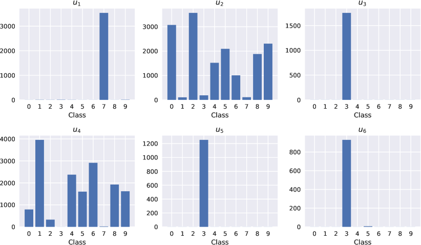
We can interpret the instance clusters by analysing their correspondence with the actual digit labels. It is then immediate to recognize that cluster $u_{1}$ corresponds to the digit 7, $u_{3}$, $u_{5}$, and $u_{6}$ all correspond to digit 3, and $u_{2}$ and $u_{4}$ correspond to digits other than 7 and 3. All correspondences are shown by histograms in Figure 6. From a decision tree trained to predict cluster identifiers of sub-bags $x_{j}$ from instance-level occurrence vectors $(o_{u_{1}},\ldots,o_{u_{6}})$ we then extract the following rules defining the function $s$:

$$\begin{array}[]{ll}1&s=v_{1}\leftarrow o_{u_{1}}\mathord{=}1,o_{u_{3}}\mathord{=}0,o_{u_{5}}\mathord{=}0,o_{u_{6}}\mathord{=}0.\\ 2&s=v_{2}\leftarrow o_{u_{1}}\mathord{=}0.\\ 3&s=v_{2}\leftarrow o_{u_{3}}\mathord{=}1.\\ 4&s=v_{2}\leftarrow o_{u_{5}}\mathord{=}1.\\ 5&s=v_{2}\leftarrow o_{u_{6}}\mathord{=}1.\\ \end{array}$$ (8)

Based on the already established interpretation of the instance clusters $u_{1},u_{3},u_{5},u_{6}$ we thus find that the sub-bag cluster $v_{1}$ gets attached to the sub-bags that contain a seven and not a three, i.e., it corresponds to the latent ’positive’ label for sub-bags.

Similarly, we extracted the following rule that predict the class label of a top-bag $x$ based on the sub-bag occurrence vector $(o_{v_{1}},o_{v_{2}})$.

$$\begin{array}[]{ll}1&t=\mbox{positive}\leftarrow o_{v_{1}}\mathord{=}1\\ 2&t=\mbox{negative}\leftarrow o_{v_{1}}\mathord{=}0\\ \end{array}$$ (9)

Hence, in this example, the true rules behind the data generation process were perfectly recovered. Note that perfect recovery does not necessarily imply perfect accuracy of the resulting rule-based classification model $r,s,t$, since the initial instance clusters $r(x_{{j},{\ell}})$ do not correspond to digit labels with 100% accuracy. Nonetheless, in this experiment the classification accuracy of the interpretable rule model on the test set was $98.18\%$, only $0.24\%$ less than the accuracy of the original model, which it approximated with a fidelity of $99.16\%$.

6.2 Sentiment Analysis

In this section, we apply our approach to a real-world dataset for sentiment analysis. The main objective of this experiment is to demonstrate the feasibility of our model interpretation framework on real-world data, and to explore the trade-offs between an MMIL and MIL approach. We use the IMDB (Maas et al., 2011) dataset, which is a standard benchmark movie review dataset for binary sentiment classification. We remark that this IMDB dataset differs from the IMDB graph datasets described in Section 6.4. IMDB consists of 25,000 training reviews, 25,000 test reviews and 50,000 unlabeled reviews. Positive and negative labels are balanced within the training and test sets. Text data exhibits a natural bags-of-bags structure by viewing a text as a bag of sentences, and each sentence as a bag of words. Moreover, for the IMDB data it is reasonable to associate with each sentence a (latent) sentiment label (positive/negative, or maybe something more nuanced), and to assume that the overall sentiment of the review is a (noisy) function of the sentiments of its sentences. Similarly, sentence sentiments can be explained by latent sentiment labels of the words it contains.

A MMIL dataset was constructed from the reviews, where then each review (top-bag) is a bag of sentences. However, instead of modeling each sentence (sub-bag) as a bag of words, we represented sentences as bags of trigrams in order to take into account possible negations, e.g. “not very good”, “not so bad”. Figure 7 depicts an example of the decomposition of a two sentence review $x$ into MMIL data.

Figure 7: A review transformed into MMIL data. The word “_” represents the padding.

Each word is represented with Glove word vectors (Pennington et al., 2014) of size 100, trained on the dataset. The concatenation of its three Glove word vectors then is the feature vector we use to represent a trigram. We here use Glove word vectors for a more pertinent comparison of our model with the state-of-the-art (Miyato et al., 2016). Nothing prevents us from using a one-hot representation even for this scenario. In order to compare MMIL against multi-instance (MIL) we also constructed a multi-instance dataset in which a review is simply represented as a bag of trigrams.

We trained two neural networks for MMIL and MIL data respectively, which have the following structure:

• MMIL network: a Conv1D layer with 300 filters (each trigram is treated separately), ReLU activations and kernel size of 100 (with stride 100), two stacked bag-layers (with ReLU activations) with 500 units each (250 max-aggregation, 250 mean-aggregation) and an output layer with sigmoid activation;

• MIL network: a Conv1D layer with 300 filters (each trigram is treated separately), ReLU activations and kernel size of 100 (with stride 100), one bag-layers (with ReLU activations) with 500 units (250 max-aggregation, 250 mean-aggregation) and an output layer with sigmoid activation;

The models were trained by minimizing the binary cross-entropy loss. We ran 20 epochs of the Adam optimizer with learning rate 0.001, on mini-batches of size 128. We used also virtual adversarial training (Miyato et al., 2016) for regularizing the network and exploiting the unlabeled reviews during the training phase. Although our model does not outperform the state-of-the-art ($94.04\%$,  Miyato et al. (2016)), we obtained a final accuracy of $92.18\pm 0.04$ for the MMIL network and $91.41\pm 0.08$ for the MIL network, by running the experiments 5 times for both the networks. Those results show that the MMIL representation here leads to a slightly higher accuracy than the MIL representation.

When accuracy is not the only concern, our models have the advantage that we can distill them into interpretable sets of rules following our general strategy. As in Section 6.1, we constructed interpretable rules both in the MMIL and in the MIL setting. Using 2,500 reviews as a validation set, we obtained in the MMIL case 4 and 5 clusters for sub-bags and instances, respectively, and in the MIL case 6 clusters for instances. Full grid search results on the validation set are reported in Appendix B (Figure 17).

In this case we interpret clusters by representative elements. Using centroids or points close to centroids as representatives here produced points (triplets, respectively sentences) with relatively little interpretative value. We therefore focused on inter-cluster separation rather than intra-cluster cohesion, and used the minimum distance to any other cluster centroid as a cluster representativeness score.

Tables 1 and 2 report the top-scoring sentences and trigrams, respectively, sorted by decreasing score. It can be seen that sentences labeled by $v_{1}$ or $v_{4}$ express negative judgments, sentences labeled by $v_{2}$ are either descriptive, neutral or ambiguous, while sentences labeled by $v_{3}$ express a positive judgment. Similarly, we see that trigrams labeled by $u_{1}$ express positive judgments while trigrams labeled by $u_{2}$ or $u_{4}$ express negative judgments. Columns printed in grey correspond to clusters that do not actually appear in the extracted rules (see below), and they do not generally correspond to a clearly identifiable sentiment. Percentages in parenthesis in the headers of these tables refer to fraction of sentences or trigrams associated with each cluster (the total number of sentences in the dataset is approximately 250 thousand while the total number of trigrams is approximately 4.5 million). A similar analysis was performed in the MIL setting (results in Table 3).

Table 1: Interpreting sentence (sub-bag) clusters in the MMIL setting.

$v_{1}$ $(11.37\%)$	$v_{2}$ $(41.32\%)$	$v_{3}$ $(15.80\%)$	$v_{4}$ $(31.51\%)$
overrated poorly written badly acted	I highly recommend you to NOT waste your time on this movie as I have	I loved this movie and I give it an 8/ 10	It’s not a total waste
It is badly written badly directed badly scored badly filmed	This movie is poorly done but that is what makes it great	Overall I give this movie an 8/ 10	horrible god awful
This movie was poorly acted poorly filmed poorly written and overall horribly executed	Although most reviews say that it isn’t that bad i think that if you are a true disney fan you shouldn’t waste your time with…	final rating for These Girls is an 8/ 10	Awful awful awful
Poorly acted poorly written and poorly directed	I’ve always liked Madsen and his character was a bit predictable but this movie was definitely a waste of time both to watch and make…	overall because of all these factors this film deserves an 8/ 10 and stands as my favourite of all the batman films	junk forget it don’t waste your time etc etc
This was poorly written poorly acted and just overall boring	If you want me to be sincere The Slumber Party Massacre Part 1 is the best one and all the others are a waste of…	for me Cold Mountain is an 8/ 10	Just plain god awful

Table 2: Interpreting trigram (instance) clusters in the MMIL setting.

$u_{1}$ $(5.73\%)$	$u_{2}$ $(8.68\%)$	$u_{3}$ $(28.86\%)$	$u_{4}$ $(2.82\%)$	$u_{5}$ $(53.91\%)$
_ 8/ 10	trash 2 out	had read online	it’s pretty poorly	give this a
an 8/ 10	to 2 out	had read user	save this poorly	like this a
for 8/ 10	_ 2 out	on IMDb reading	for this poorly	film is 7
HBK 8/ 10	a 2 out	I’ve read innumerable	just so poorly	it an 11
Score 8/ 10	3/5 2 out	who read IMDb	is so poorly	the movie an
to 8/ 10	2002 2 out	to read IMDb	were so poorly	this movie an
verdict 8/ 10	garbage 2 out	had read the	was so poorly	40 somethings an
Obscura 8/ 10	Cavern 2 out	I’ve read the	movie amazingly poorly	of 5 8
Rating 8/ 10	Overall 2 out	movie read the	written poorly directed	gave it a
it 8/ 10	rating 2 out	Having read the	was poorly directed	give it a
fans 8/ 10	film 2 out	to read the	is very poorly	rating it a
Hero 8/ 10	it 2 out	I read the	It’s very poorly	rated it a
except 8/ 10	score 2 out	film reviews and	was very poorly	scored it a
Tracks 8/ 10	Grade 2 out	will read scathing	a very poorly	giving it a
vote 8/ 10	Just 2 out	_ After reading	very very poorly	voting it a
as 8/ 10	as 2 out	about 3 months	Poorly acted poorly	are reasons 1
strong 8/ 10	and 2 out	didn’t read the	are just poorly	it a 8
rating 8/ 10	rated 2 out	even read the	shown how poorly	vote a 8
example 8/ 10	Rating 2 out	have read the	of how poorly	a Vol 1
… 8/ 10	conclusion 2 out	the other posted	watching this awful	this story an

Table 3: Interpreting trigram (instance) clusters in the MIL setting.

$u_{1}$ $(13.53\%)$	$u_{2}$ $(41.53\%)$	$u_{3}$ $(3.03\%)$	$u_{4}$ $(5.47\%)$	$u_{5}$ $(31.58\%)$	$u_{6}$ $(4.85\%)$
production costs _	give it a	only 4/10 _	is time well-spent	… 4/10 …	_ Recommended _
all costs _	gave it a	score 4/10 _	two weeks hairdressing	.. 1/10 for	Highly Recommended _
its costs _	rated it a	a 4/10 _	2 hours _	rate this a	Well Recommended _
ALL costs _	rating it a	_ 4/10 _	two hours _	gave this a	_ 7/10 _
possible costs _	scored it a	average 4/10 _	finest hours _	give this a	13 7/10 _
some costs _	giving it a	vote 4/10 _	off hours _	rated this a	rate 7/10 _
cut costs _	voting it a	Rating 4/10 _	few hours _	_ Not really	.. 7/10 _
rate this a	gave this a	.. 4/10 _	slow hours _	4/10 Not really	this 7/10 _
gave this a	give this a	is 4/10 _	three hours _	a 4/10 or	Score 7/10 _
rating this a	rate this a	this 4/10 _	final hours _	of 4/10 saying	solid 7/10 _
give this a	giving this a	of 4/10 _	early hours _	rate it a	a 7/10 _
and this an	gives this a	movie 4/10 _	six hours _	give it a	rating 7/10 _
give this an	like this a	verdict 4/10 _	48 hours _	gave it a	to 7/10 _
given this an	film merits a	gave 4/10 _	4 hours _	given it a	viewing 7/10 _
gave this an	Stupid Stupid Stupid	13 4/10 _	6 hours _	giving it a	it 7/10 _
rating this an	_ Stupid Stupid	disappointment 4/10 _	five hours _	scored it a	score 7/10 _
rate this an	award it a	at 4/10 _	nocturnal hours _	award it a	movie 7/10 _
all costs …	given it a	rating 4/10 _	17 hours _	Cheesiness 0/10 Crappiness	is 7/10 _
all costs ..	makes it a	… 4/10 _	for hours _	without it a	drama 7/10 _
_ Avoid _	Give it a	rate 4/10 _	wasted hours _	deserves 4/10 from	Recommended 7/10 _

MMIL rules

Using a decision tree learner taking frequency vectors $(f_{u_{1}},\ldots,f_{u_{5}})$ as inputs, we obtained the rules reported in Table 4.

Table 4: MMIL rules mapping instance cluster frequencies ($f_{u_{i}}$) into sub-bag cluster identifiers. Numbers express percentages and rules are written as definite clauses in a Prolog-like syntax where $\leftarrow$ is the implication and conjuncted literals are joined by a comma.

$$\begin{array}[]{ll}\hline\cr\hline\cr 1&v_{1}\leftarrow f_{u_{1}}\mathord{\leq}6.03,f_{u_{2}}\mathord{>}10.04,f_{u_{4}}\in(2.77,12.59].\\ 2&v_{1}\leftarrow f_{u_{1}}\mathord{\leq}16.90,f_{u_{4}}\mathord{>}12.59.\\ {\color[rgb]{0.56640625,0.56640625,0.56640625}\definecolor[named]{pgfstrokecolor}{rgb}{0.56640625,0.56640625,0.56640625}3}&{\color[rgb]{0.56640625,0.56640625,0.56640625}\definecolor[named]{pgfstrokecolor}{rgb}{0.56640625,0.56640625,0.56640625}v_{2}\leftarrow f_{u_{1}}\mathord{\leq}8.43,f_{u_{2}}\mathord{\leq}8.88,f_{u_{4}}\mathord{\leq}2.77}.\\ {\color[rgb]{0.56640625,0.56640625,0.56640625}\definecolor[named]{pgfstrokecolor}{rgb}{0.56640625,0.56640625,0.56640625}4}&{\color[rgb]{0.56640625,0.56640625,0.56640625}\definecolor[named]{pgfstrokecolor}{rgb}{0.56640625,0.56640625,0.56640625}v_{2}\leftarrow f_{u_{1}}\mathord{>}3.20,f_{u_{2}}\in(8.88,20.39],f_{u_{4}}\mathord{\leq}2.77}.\\ {\color[rgb]{0.56640625,0.56640625,0.56640625}\definecolor[named]{pgfstrokecolor}{rgb}{0.56640625,0.56640625,0.56640625}5}&{\color[rgb]{0.56640625,0.56640625,0.56640625}\definecolor[named]{pgfstrokecolor}{rgb}{0.56640625,0.56640625,0.56640625}v_{2}\leftarrow f_{u_{1}}\mathord{>}6.03,f_{u_{2}}\mathord{\leq}6.03,f_{u_{4}}\in(2.77,12.59]}.\\ 6&v_{3}\leftarrow f_{u_{1}}\mathord{>}8.43,f_{u_{2}}\mathord{\leq}8.88,f_{u_{4}}\mathord{\leq}2.77.\\ 7&v_{4}\leftarrow f_{u_{1}}\mathord{\leq}3.20,f_{u_{2}}\mathord{>}8.88,f_{u_{4}}\mathord{\leq}2.77.\\ 8&v_{4}\leftarrow f_{u_{1}}\mathord{>}3.20,f_{u_{2}}\mathord{>}20.39,f_{u_{4}}\mathord{\leq}2.77.\\ 9&v_{4}\leftarrow f_{u_{1}}\mathord{\leq}6.03,f_{u_{2}}\mathord{\leq}10.04,f_{u_{4}}\in(2.77,12.59].\\ 10&v_{4}\leftarrow f_{u_{1}}\mathord{>}6.03,f_{u_{2}}\mathord{>}6.03,f_{u_{4}}\in(2.77,12.59].\\ 11&v_{4}\leftarrow f_{u_{1}}\mathord{>}16.90,f_{u_{4}}\mathord{>}12.59.\\ \hline\cr\hline\cr\end{array}$$

Even though these rules are somewhat more difficult to parse than the ones we obtained in Section 6.1, they still express relatively simple relationships between the triplet and sentence clusters. Especially the single sentence cluster $v_{3}$ that corresponds to a clearly positive sentiment has a very succinct explanation given by the rule of line 6. Rules related to sentence cluster $v_{2}$ are printed in grey. Since $v_{2}$ is not used by any of the rules shown in Table 5 that map sub-bag (sentence) cluster identifiers to the top-bag (review) class labels, the rules for $v_{2}$ will never be required to explain a particular classification.

Table 5: MMIL rules mapping sentence cluster frequencies into review sentiment labels. See the caption of Table 4 for details on the syntax.

$$\begin{array}[]{ll}\hline\cr\hline\cr 1&\mbox{positive}\leftarrow f_{v_{1}}\mathord{\leq}4.04,f_{v_{3}}\mathord{\leq}12.63,f_{v_{4}}\mathord{\leq}39.17.\\ 2&\mbox{positive}\leftarrow f_{v_{1}}\mathord{\leq}12.97,f_{v_{3}}\mathord{>}12.63.\\ 3&\mbox{positive}\leftarrow f_{v_{1}}\mathord{>}12.97,f_{v_{3}}\mathord{>}25.66.\\ 4&\mbox{negative}\leftarrow f_{v_{1}}\mathord{\leq}4.04,f_{v_{3}}\mathord{\leq}12.63,f_{v_{4}}\mathord{>}39.17.\\ 5&\mbox{negative}\leftarrow f_{v_{1}}\mathord{>}4.04,f_{v_{3}}\mathord{\leq}12.63.\\ 6&\mbox{negative}\leftarrow f_{v_{1}}\mathord{>}12.97,f_{v_{3}}\in(12.63,25.66].\\ \hline\cr\hline\cr\end{array}$$

MIL rules.

For the MIL model, rules map a bag $x$, described by its instance frequency vector $(f_{u_{1}},\ldots,f_{u_{5}})$, to the bag class label. They are reported in Table 6. Note that only two out of the six instance clusters are actually used in these rules.

Table 6: MIL classification rules. See the caption of Table 4 for details on the syntax.

$$\begin{array}[]{ll}\hline\cr\hline\cr 1&\mbox{positive}\leftarrow f_{u_{3}}\mathord{\leq}1.11,f_{u_{6}}\mathord{\leq}3.42.\\ 2&\mbox{positive}\leftarrow f_{u_{3}}\mathord{\leq}2.21,f_{u_{6}}\mathord{>}3.42.\\ 3&\mbox{positive}\leftarrow f_{u_{3}}\in(2.21,5.81],f_{u_{6}}\mathord{>}6.30.\\ 4&\mbox{negative}\leftarrow f_{u_{3}}\in(1.11,2.21],f_{u_{6}}\mathord{\leq}3.42.\\ 5&\mbox{negative}\leftarrow f_{u_{3}}\mathord{>}2.21,f_{u_{6}}\mathord{\leq}6.30.\\ 6&\mbox{negative}\leftarrow f_{u_{3}}\mathord{>}5.81,f_{u_{6}}\mathord{>}6.30.\\ \hline\cr\hline\cr\end{array}$$

By classifying IMDB using the rules and cluster identifiers, we achieved an accuracy of $87.49\%$ on the test set for the MMIL case and $86.37\%$ for the MIL case. Fidelities in the MMIL and in the MIL settings were $90.40\%$ and $88.10\%$, respectively. We thus see that the somewhat higher complexity of the rule-based explanation of the model learned in the MMIL setting also corresponds to a somewhat higher preservation of accuracy. As we demonstrate by the following example, the multi-level explanations derived from model learned in the MMIL setting can also lead to more transparent explanations for individual predictions.

An example of prediction explanation.

As an example we consider a positive test-set review for the movie Bloody Birthday, which was classified correctly by the MMIL rules and incorrectly by the MIL rules. Its full text is reported in Table 7. Classification in the MMIL setting was positive due to applicability of rule 2 in Table 5. This rule only is based on sentences in clusters $v_{1}$ and $v_{3}$, and therefore sentences assigned in any other cluster do not actively contribute to this classification. These irrelevant sentences are dimmed in the printed text (Table 7, top part). A first, high-level explanation of the prediction is thus obtained by simply using the sentences that are active for the classification as a short summary of the most pertinent parts of the review.

This sentence-level explanation can be refined by also explaining the clusters for the individual sentences. For example, sentence “Bloody Birthday a $\dots$” was assigned to identifier $v_{1}$ using rule 2 of Table 4. This rule is based on frequencies of the trigram cluster identifiers $u_{1}$ and $u_{4}$. Occurrences of trigrams with these identifiers are highlighted in boldface and superscripted with the trigram cluster identifier in the text, thus exhibiting the sub-structures in the sentence that are pertinent for the classification. Similarly, the other three relevant sentences were all assigned to identifier $v_{3}$ because of rule 6 in Table 4, which is based on identifiers $u_{1},u_{2},u_{4}$. These formal, logical explanations for the classifications are complemented by the semantic insight into the cluster identifiers provided by Tables 2 and 1.

The review was classified as negative in the MIL setting. The applicable rule here was rule 5 in Table 6 which involved triplet identifiers $u_{3}$, and $u_{6}$. The relevant triplets are highlighted in boldface in the lower part of Table 7.

A second example of prediction explanation is reported in Appendix B.

Table 7: A sample positive review. Top: MMIL labeling. Bottom: MIL labeling.

6.3 Citation Datasets

In the following experiments, we apply MMIL to graph learning according to the general strategy described in Section 3. We also present a (generalized) MIL approach to graph learning in which latent instance labels need not be binary, and need not be related to the bag label according to the conventional MIL rule. We considered three citation datasets from (Sen et al., 2008): Citeseer, Cora, and PubMed. Finally, the MMIL network trained on PubMed will be mapped into an interpretable model using the procedure described in Section 4.

We view the datasets as graphs where nodes represent papers described by titles and abstracts, and edges are citation links. We treat the citation links as undirected edges, in order to have a setup as close as possible to earlier works, (Kipf and Welling, 2016; Hamilton et al., 2017). The goal is to classify papers according to their subject area.

We collected the years of publication for all the papers of each dataset, and for each dataset determined two thresholds $yr_{1}<yr_{2}$, so that papers with publication year $yr\leq yr_{1}$ amount to approximately $40\%$ of the data and are used as the training set, papers with publication year $yr_{1}<yr\leq yr_{2}$ formed a validation set of about $20\%$, and papers with publication year $yr>yr_{2}$ are the test set of $40\%$ of the data. Table 8 reports the statistics for each dataset. More details on the temporal distributions in the three datasets are given in Appendix C (Figure 18). This particular split is justified by the fact that we would like to evaluate those datasets in a more realistic and challenging scenario, where we used past publications to predict the class of the new ones. Furthermore, CiteSeer, Cora, and PubMed are typically evaluated in a transductive setting, where the feature vectors, associated with the test set nodes, are allowed to be used during the training. Here, instead, we consider an inductive setup, where the test set nodes remain unobserved during the training. However, for an exhaustive comprehension, we evaluated the three datasets considering also 10 random splits (with the same proportions reported in Table 8) while maintaining the inductive setting.

Table 8: Structure of the citation graphs. With $yr$ we denote the year of publication. Citeseer classes are 6 among Agents, Artificial Intelligence (AI), Database (DB), Human-computer Interaction (HCI), Information Retrieval (IR), Machine Learning (ML). Cora classes are 7 among Case Based, Genetic Algorithms, Neural Networks, Probabilist Methods, Reinforcement Learning, Rule Learning, Theory. PubMed classes are 3 among Diabetes Mellitus Experimental (DME), Diabetes Mellitus Type 1 (DMT1), Diabetes Mellitus Type 2(DMT2).

Dataset	# Classes	# Nodes	# Edges	# Training	# Validation	# Test
CiteSeer	6	3,327	4,732	1,560	779	988
				$(yr\leq`99)$	$(`99<yr\leq`00)$	$(yr>`00)$
Cora	7	2,708	5,429	1,040	447	1,221
				$(yr\leq`94)$	$(`94<yr\leq`95)$	$(yr>`95)$
PubMed	3	19,717	44,338	8,289	3,087	8,341
				$(yr\leq`97)$	$(`97<yr\leq`01)$	$(yr>`01)$

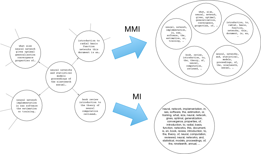
MMIL data was constructed from citation networks in which a top-bag $x$ corresponds to a paper represented as the bag of nodes $x_{j}$ containing the paper itself and all its neighbors. The nodes $x_{j}\in x$ are further decomposed as (sub-) bags of the words contained in the text (i.e. title and abstract) attached to the node. An instance $x_{{j},{\ell}}\in x_{j}$ is a word. Similarly, MIL data was constructed in which each paper is simply represented as the bag of all words appearing in the text of the paper or its neighbors. Figure 8 shows an example of MMIL and MIL decompositions starting from a node and its neighborhood of a citation graph. Words are encoded as one-hot vectors, in order to evaluate the capability of our model to learn relevant intermediate representations of bags from scratch.

Figure 8: Given node an its neighborhood of a citation graph (left picture) we decomposed it as MMIL data (upper right picture) and MIL data (bottom right picture).

We used an MMIL network model with two stacked bag-layers with ReLU activations with 250 units. The MIL model has one bag-layer with ReLU activations with 250 units. For both MMIL and MIL we proposed two versions which differ only for the aggregation functions for the bag-layers: one version uses max, the other uses mean aggregation. All models were trained by minimizing the softmax cross-entropy loss. We ran 100 epochs of the Adam optimizer with learning rate 0.001 and we early stopped the training according to the loss on the validation set.

As baselines, we considered Näive Bayes and logistic regression. For these two models we reduced the task to a standard classification problem in which papers are represented by bag of words feature vectors (only for the words associated with the papers themselves, not considering citation neighbors). We also compared our models against GCN (Kipf and Welling, 2016), GraphSAGE (Hamilton et al., 2017) and GAT (Velickovic et al., 2018), which are briefly described in Section 5. GCN and GAT represent nodes as bags of words, while GraphSAGE exploits the sentence embedding approach described by (Arora et al., 2016). For comparison reasons and given that bag of words represent the most challenging and standalone approach which does not rely in any embedding representation of words, we encoded the nodes as bag of words for GCN, GraphSAGE, and GAT. As GraphSAGE allows to use both max and mean as aggregation functions, we compared our models against both versions, with a subsampling neighbor size of 25.

Results in Table 9 report the accuracy and the standard deviation for all the models. The columns Temp refer to our temporal splits, while the columns Rnd refer to random splits. The random splits are kept fixed for all the experiments. The standard deviations are evaluated on 10 restarts for the Temp and on 10 randoms splits for the Rnd. The MMIL networks outperform the other methods. MIL networks show a similar performance to GCN, GraphSage and GAT on Cora and Citeseer, and are close to MMIL on PubMed. It is noteworthy that the quite generic MMIL framework which here only is instantiated for graph data as a special case outperforms the methods that are specifically designed for graphs. urthermore, the experimental results suggest that the temporal splits provide a more challenging task than random splits. Finally, as typically Cora, CiteSeer, and PubMed are used in the transductive setup we also report in Table 10 the results for this setting. Here we used the same splits described in Kipf and Welling (2016) and Velickovic et al. (2018). MMIL-Mean achieved comparable results with GCN and slightly worse than GAT. Hyperparameters for models appearing in both Table 9, and 10 are the same and they come from the respective papers.

Table 9: Inductive setting. Accuracies with standard deviations on the test sets. Best results are highlighted in bold.

Model	Cora		CiteSeer		PubMed
	Temp	Rnd	Temp	Rnd	Temp	Rnd
N. Bayes	71.3	$73.8\pm 1.4$	63.8	$71.6\pm 1.0$	75.5	$79.4\pm 0.5$
Log Reg	74.9	$76.5\pm 1.0$	64.4	$71.1\pm 1.7$	73.7	$86.0\pm 0.3$
GCN	$81.2\pm 0.7$	$83.7\pm 0.8$	$66.4\pm 0.6$	$73.6\pm 1.5$	$78.0\pm 1.0$	$83.7\pm 0.3$
GS-Mean	$80.1\pm 0.8$	$83.4\pm 1.1$	$65.3\pm 1.6$	$73.6\pm 0.6$	$75.4\pm 0.9$	$83.8\pm 0.4$
GS-Max	$80.0\pm 0.7$	$83.4\pm 1.1$	$65.3\pm 1.2$	$73.3\pm 1.1$	$74.3\pm 0.7$	$83.9\pm 0.6$
GAT	$80.2\pm 2.4$	$82.0\pm 1.7$	$68.2\pm 1.8$	$68.7\pm 1.7$	$80.8\pm 1.4$	$84.9\pm 0.8$
Mil-Mean	$81.0\pm 1.0$	$84.0\pm 1.4$	$70.2\pm 0.6$	$\bm{75.5\pm 1.5}$	$80.1\pm 0.9$	$\bm{86.2\pm 0.2}$
Mil-Max	$81.3\pm 0.8$	$83.8\pm 1.2$	$68.7\pm 0.8$	$75.0\pm 1.2$	$79.2\pm 0.9$	$84.7\pm 0.6$
Mmil-Mean	$83.0\pm 0.9$	$83.3\pm 1.2$	$\bm{71.3\pm 1.1}$	$74.5\pm 1.6$	$\bm{82.4\pm 0.9}$	$86.0\pm 0.3$
Mmil-Max	$\bm{83.6\pm 0.5}$	$\bm{84.1\pm 1.5}$	$70.1\pm 0.6$	$75.0\pm 1.4$	$79.0\pm 1.7$	$85.0\pm 0.7$

Table 10: Transductive setting. Accuracies with standard deviations on the test sets. Best results are highlighted in bold.

Model	Cora	CiteSeer	PubMed
GCN	$81.5$	$70.3$	$79.0$
GAT	$83.0\pm 0.7$	$72.5\pm 0.7$	$79.0\pm 0.3$
Mil-Mean	$78.5\pm 0.7$	$66.8\pm 0.9$	$77.1\pm 0.5$
Mil-Max	$75.7\pm 0.9$	$66.8\pm 1.1$	$73.1\pm 0.6$
Mmil-Mean	$82.1\pm 0.5$	$69.7\pm 0.4$	$78.1\pm 0.3$
Mmil-Max	$77.9\pm 0.7$	$66.6\pm 1.2$	$73.4\pm 0.6$

Our general approach to interpretability can also be applied to models learned in the MIL and in the MMIL settings for the citation graphs. The associated interpretability study on PubMed data is reported in Appendix C.

6.4 Social Network Datasets

We finally test our model on a slightly different type of prediction problems for graph data, where the task is graph classification, rather than node classification as in the previous section. For this we use the following six publicly available datasets first proposed by Yanardag and Vishwanathan (2015).

• COLLAB is a dataset where each graph represent the ego-network of a researcher, and the task is to determine the field of study of the researcher, which is one of High Energy Physics, Condensed Matter Physics, or Astro Physics.

• IMDB-BINARY, IMDB-MULTI are datasets derived from IMDB. First, genre-specific collaboration networks are constructed where nodes represent actors/actresses who are connected by an edge if they have appeared together in a movie of a given genre. Collaboration networks are generated for the genres Action and Romance for IMDB-BINARY and Comedy, Romance, and Sci-Fi for IMDB-MULTI. The data then consists of the ego-graphs for all actors/actresses in all genre networks, and the task is to identify the genre from which an ego-graph has been extracted.

• REDDIT-BINARY, REDDIT-MULTI5K, REDDIT-MULTI12K are datasets where each graph is derived from a discussion thread from Reddit. In those graphs each vertex represent a distinct user and two users are connected by an edge if one of them has responded to a post of the other in that discussion. The task in REDDIT-BINARY is to discriminate between threads originating from a discussion-based subreddit (TrollXChromosomes, atheism) or from a question/answers-based subreddit (IAmA, AskReddit).

  The task in REDDIT-MULTI5K and REDDIT-MULTI12K is a multiclass classification problem where each graph is labeled with the subreddit where it has originated (worldnews, videos, AdviceAnimals, aww, mildlyinteresting for REDDIT-MULTI5K and AskReddit, AdviceAnimals, atheism, aww, IAmA, mildlyinteresting, Showerthoughts, videos, todayilearned, worldnews, TrollXChromosomes for REDDIT-MULTI12K).

We transformed each dataset into MMIL data by treating each graph as a top-bag $x$. Each node of the graph with its neighborhood, is a sub-bag $x_{j}\in x$ while each node $x_{{j},{\ell}}\in x_{j}$ is an instance.

In these six datasets no features are attached to the nodes. We therefore defined a node feature vector based on the degrees $deg(x_{{j},{\ell}})$ of the nodes as follows: let $deg^{*}$ be the maximum degree of any node. For $i=1,\ldots,deg^{*}$ we then define

$$x_{{j},{\ell}}^{i}=\begin{cases}\frac{1}{\sqrt{deg(x_{{j},{\ell}})}}&\quad if\ i<deg(x_{{j},{\ell}})\\ 0&\quad otherwise,\end{cases}$$ (10)

By using this representation the scalar product of two node feature vectors will be high if the nodes have similar degrees, and it will be low for nodes with very different degrees.

The MMIL networks have the same structure for all the datasets: a dense layer with 500 nodes and ReLU activation, two stacked bag-layers with 500 units (250 max units and 250 mean units), and a dense layer with $dim_{out}$ nodes and linear activation, where $dim_{out}$ is $3$ for COLLAB, $2$ for IMDB-Binary, and $3$ for IMDB-MULTI, $2$ for REDDIT-BINARY, $5$ for REDDIT-MULTI5K, and $11$ for REDDIT-MULTI12K. We performed a 10 times 10 fold cross-validation, training the MMIL networks by minimizing the binary cross-entropy loss (for REDDIT-BINARY and IMDB-BINARY) and the softmax cross-entropy loss (for COLLAB, IMDB-MULTI, REDDIT-5K, REDDIT-12K). We ran 100 epochs of the Adam optimizer with learning rate 0.001 on mini-batches of size 20.

We compared our method against DGK (Yanardag and Vishwanathan, 2015), Patchy-SAN (Niepert et al., 2016), and SAEN (Orsini et al., 2018).

Table 11: Accuracies with standard deviations in graph classification. Best results are highlighted in bold.

Dataset	DGK	Patchy-SAN	SAEN	MMIL
Collab	$73.09\pm 0.25$	$72.60\pm 2.15$	$78.50\pm 0.69$	$\bm{79.46\pm 0.31}$
Imdb-Binary	$66.96\pm 0.56$	$71.00\pm 2.29$	$71.59\pm 1.20$	$\bm{72.62\pm 1.04}$
Imdb-Multi	$44.55\pm 0.52$	$45.23\pm 2.84$	$48.53\pm 0.76$	$\bm{49.42\pm 0.68}$
Reddit-Binary	$78.04\pm 0.39$	$86.30\pm 1.58$	$\bm{87.22\pm 0.80}$	$86.54\pm 0.64$
Reddit-Multi5k	$41.27\pm 0.18$	$49.10\pm 0.70$	$\bm{53.63\pm 0.51}$	$53.42\pm 0.67$
Reddit-Multi12k	$32.22\pm 0.10$	$41.32\pm 0.42$	$\bm{47.27\pm 0.42}$	$45.25\pm 0.48$

Results in Table 11 show that MMIL networks and SAEN perform comparably, with some advantages of these two methods over Patch-SAN, and more pronounced advantages over DGK.

6.5 Point Clouds

Following the experiments reported in (Zaheer et al., 2017), we aim at illustrating the benefits of the MMIL setting for point clouds datasets and at demonstrating results of our interpretation framework. We start from the ModelNet40 dataset (Wu et al., 2015) which consists of $9,843$ training and $2,468$ test point clouds of objects distributed over $40$ classes. The dataset is preprocessed with the same procedure described by Zaheer et al. (2017). To investigate the effect of spatial resolution, we produce point clouds with 100 and 5,000 three-dimensional points (instances) from the mesh representation of objects using the point-cloud library’s sampling routine (Rusu and Cousins, 2011). Each set is normalized to have zero mean (along individual axes) and unit (global) variance. We call P100 and P5000 the two datasets, which are readily usable for the MIL setting (or DeepSets).

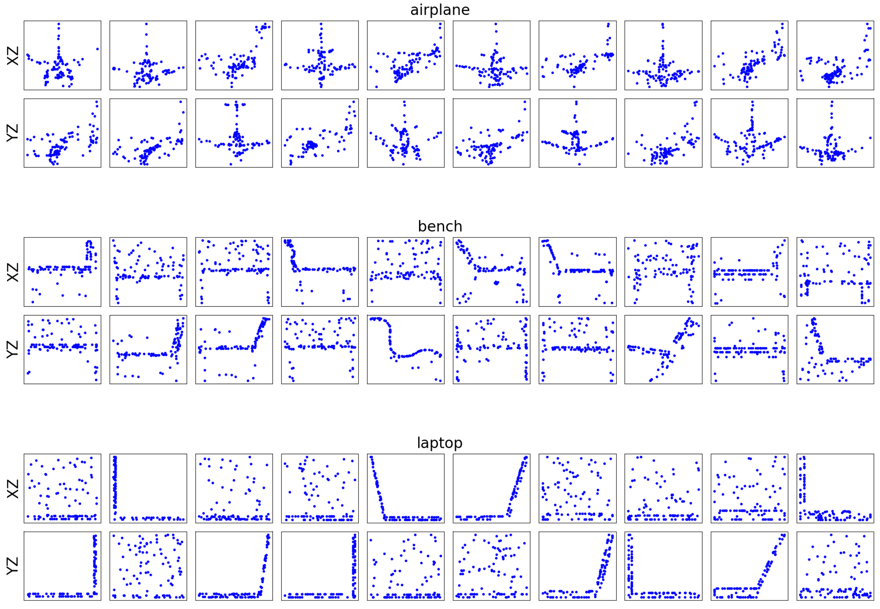
The orientations of the point clouds in the dataset are different as clearly shown in Figure 9, where we reported the projections on the XZ and YZ planes of some point clouds drawn from airplane, bench, and laptop classes. Each column of each class represents the same point cloud projected into the XZ and YZ planes, respectively. Methods that do not take into account this fact might encounter difficulties. On other hand, the bags-of-bags representation is a very natural way to effectively handle different orientations for this dataset. Therefore, we subsequently created bags of bags by considering $R$ equally distributed rotations, i.e. $\{\frac{2\pi i}{R}\}_{i=1}^{N}$, around the $z$-axis. We used $R=5$ in P100 and $R=16$ in P5000. A top-bag $x$ is thus a set of rotated versions of the same point cloud, i.e. a set of sub-bags $x_{j}\in x,\ j=1,\dots,R$.

Figure 9: Examples of point clouds projected into the XZ and YZ planes.

In the MMIL setting, networks have exactly the same structure (and the same hyper-parameters) of the DeepSets permutation invariant model described by Zaheer et al. (2017), except for adding a further Bag-Layer of $40$ sum units before the last layer. We compare our MMIL results against the DeepStets results reported in (Zaheer et al., 2017) but also against DeepSets trained on the “augmented” datasets obtained by flattening the MMIL datasets at the level of subbags. Results in Table 12 show that in both datasets there is an advantage in using the MMIL setting and the difference is more pronounced at low spatial resolution (i.e. on the P100 dataset).

We applied our interpretability approach also to the P100 dataset, whose study is reported in Appendix D.

Table 12: Accuracies with standard deviations for the ModelNet40 dataset. Best results are highlighted in bold.

Model	Dataset	Accuracy
MIL (DeepSets)	P100	$82.00+2.00\%$
MIL (DeepSets)	P100 w/ rotations	$85.35\pm 0.49\%$
MMIL	P100 bags-of-bags	$\bm{88.10\pm 0.43\%}$
MIL (DeepSets)	P5000	$90.00+0.30\%$
MIL (DeepSets)	P5000 w/ rotations	$89.28\pm 0.39\%$
MMIL	P5000 bags-of-bags	$\bm{91.17\pm 0.47\%}$

6.6 Plant Distribution Data

In this section we apply our MMIL framework to a botanical dataset containing plant species distribution data for Germany (geo, ). In this data, Germany is divided on a regular grid into 12,948 geographic regions. For each region $i$ and each of 4,842 different plant species $j$ the data contains a binary variable $a_{ij}$ indicating whether species $j$ has been observed to occur in region $i$. In addition, for each regions $i$ the data provides the latitude and longitude of $i$’s center. For our experiments, we reduced the data by selecting only the 842 most frequent species, which includes all plants that occur in at least 10 % of the regions. Deleting all regions that then do not contain any of the 842 selected species, also leads to a slight reduction in the number of regions to 12,665. The data is based on observations in the field by human experts, and is very unlikely to be completely correct. In particular, some occurrences of a species will be overlooked, leading to false negatives $a_{ij}=0$ in the data (there can also be false positives, but these can be assumed to be much more rare). The real-world task is to identify the most likely false negatives in the data, which could guide efforts to improve data completeness by additional field studies. We observe that our task is very similar to recommendation problems from binary, positive-only data (Verstrepen et al., 2017). The main difference to a generic collaborative filtering setting lies in the fact that in addition to the pure occurrence matrix $A$ we also can use the known spatial relationships between regions. In the following, we consider methods that do or do not try to exploit the spatial information. Methods of the latter type can be applied to a multitude of similarly structured recommendation problems.

Since we lack the ground truth complete data, we proceed as follows to evaluate the potential of different prediction techniques with regard to the real-world task: let $A=(a_{ij})\in\{0,1\}^{12,665\times 842}$ denote the original data. We take $A$ as a surrogate for the ground truth, and construct incomplete versions $A^{P}$ of $A$ by randomly setting for each plant $j$ $P\%$ of the occurrences $a_{ij}=1$ to $a^{P}_{ij}=0$. We constructed such matrices $A^{P}\in\{0,1\}^{12,665\times 842}$ for $P\in\{5,10,15,20,25,30\}$.

We now consider methods that using $A^{P}$ as training data compute for each pair $(i,j)$ a score $\hat{a}_{ij}$ for the actual occurrence of $j$ at $i$. We evaluate the methods based on how highly the false 0’s of $A^{P}$ are ranked by $\hat{a}_{ij}$. Concretely, for a fixed region $i$ let $Z_{i}:=\{j|a^{P}_{ij}=0\}$ and $Q_{i}:=\{j\in Z_{i}|a_{ij}=1\}$. For $j\in Z_{i}$ let $\rho(j)$ be the rank of $j$ when $Z_{i}$ is sorted according to the scores $\hat{a}_{ij}$. We then define the mean average precision for the scores at region $i$ as

$$mAP_{i}=\frac{1}{|Q_{i}|}\sum\limits_{i=1}^{|Q_{i}|}\frac{1}{i}\sum\limits_{r=1}^{i}a_{i\rho^{-1}(r)}.$$ (11)

$mAP_{i}$ attains a maximal value of 1 if the plants $j\in Q_{i}$ are exactly the highest scoring species in $Z_{i}$. Note that $mAP_{i}$ does not depend on the score values $\hat{a}_{ij}$ for species $j$ with $a^{P}_{ij}=1$. For an overall evaluation, we take the average of the $mAP_{i}$ over all regions $i$.

Several methods will depend on proximity measures between regions $i_{1}$ and $i_{2}$. In the following, $a_{i*}$ denotes the $i$th row in the matrix $A$. We consider the following two metrics:

• Hamming distance: the Hamming distance between the vectors $a^{P}_{i_{1}*}$ and $a^{P}_{i_{2}*}$.

• Euclidean distance: latitude and longitude of $i_{1},i_{2}$ are converted into Cartesian coordinates, and then Euclidean metric is applied.

Note that only Euclidean distance exploits the available spatial information.

From $A^{P}$ we created a MMIL dataset as follows: each region $i$ is a top-bag. Each plant $j$ with $a^{P}_{ij}=1$ is a sub-bag of $i$. The instances contained in a sub-bag $j$ are again regions: among all regions $i^{\prime}$ with $a^{P}_{i^{\prime}j}=1$ we include in $j$ the 25 regions with minimal Hamming distance to $i$. We also created MIL dataset where we simply merge all the sub-bags of the MMIL dataset. We compare both MIL and MMIL models against two Näive models, Gaussian processes for binary classification (Williams and Rasmussen, 2006), and matrix factorization (Zhou et al., 2008).

• Näive 1. For each region $i$, we first select the 25 closest regions ${k_{1}},\ldots,{k_{25}}$ according to the Hamming distance, and then define $\hat{a}_{i*}=\frac{1}{25}\sum_{t=1}^{25}a_{k_{t}*}$.

• Näive 2. As Näive 1, but closest regions are selected according to Euclidean distance: all neighboring regions with a Euclidean distance below a certain threshold are selected, where the threshold is set such that most regions have approximately 25 neighbors.

• Gaussian processes, (also known as kriging when applied to geostatistical problems, see e.g. Oliver and Webster (1990)). For each different plant we trained a separate Gaussian process model using the approach described by Hensman et al. (2015) and implemented by Gardner et al. (2018) within an efficient PyTorch framework. The models take as input the coordinates (representing a region) and outputs a real value between 0 and 1, which indicates the probability of the existence of the plants for the given inputs. We used the Mercer kernel as results of an hyper-parameter search.

• Matrix factorization. Motivated by the collaborative filtering analogy, we also considered a matrix factorization approach computing

  $$A^{P}\simeq U^{T}V=:\hat{A}$$

  with $U\in\{0,1\}^{12,665\times k},V\in\{0,1\}^{k\times 842}$ for some $k$ learned by minimizing a regularized sum of squared errors loss function. Hyperparameters $k$ and $\lambda_{1},\lambda_{2}$ for the matrix norms of $U$ and $V$ in the regularization term were determined through grid search as $k=50$, $\lambda_{1}=0$, $\lambda_{2}=0$.

• MMIL and MIL networks. We used a MMIL network model with two stacked bag-layers (only for the MIL network) with ReLU activations with 128 units and max as aggregation functions. On top of the bag-layers we used a dense layer with 128 units and ReLU activations, followed by the output dense layer with 842 units (corresponding to the number of plants) and sigmoid activations. Both the models are trained by minimizing the binary cross entropy loss for 100 epochs with Adam optimizer (learning rate $0.001$ until the 80th epoch and then $0.0001$) on batches of size 64.

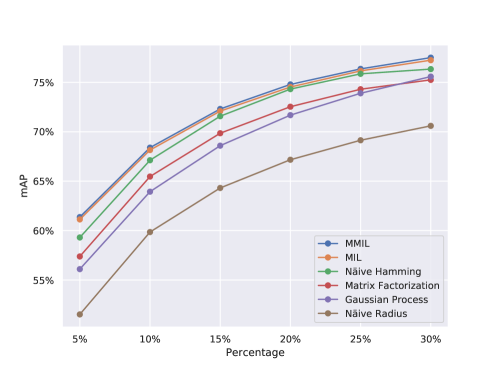
Results with respect the mAP measure (see Equation 11) are depicted in Figure 10. We can notice that MMIL and MIL outperforms the other models. Even though the difference between MMIL and MIL is small, it is consistent: we ran 6 repetitions of the experiment both for MMIL and MIL with different random initializations, and the best result of MIL was still worse than the worst result of MMIL. Among the alternative methods the naive Hamming approach showed the strongest performance by far. For most percentage values $P$ of deleted species there is still a marked gap between naive Hamming and the MI approaches. It is notable that methods that use the spatial information (Gaussian process, naive radius) perform generally worse than methods only based on the occurrence matrix $A$.

Figure 10: mAP for the all the methods and for all the datasets.

Even though our primary objective is ranking, we can also use all models as classifiers by setting a threshold for the scores $\hat{a}_{ij}$. For the following we selected one plant $j$=Vicia Villosa, used the scores learned from $A^{5}$, and determined for each method an optimal threshold for $\hat{a}_{ij}$ for predicting $a_{ij}=1$. Figure 11 shows the true distribution and the distributions predicted by MMIL, Gaussian processes, and matrix factorization.

Figure 11: True and predicted distributions of Vicia Villosa.

We also use the classification problem for Vicia Villosa to illustrate the interpretability of the MMIL model. Using 1,000 regions as validation set we obtained an optimal number of 6 and 8 clusters for sub-bags and instances, respectively. The decision tree had fidelity of $81.57\%$.

Figure 12: Visualization of the instance clusters: left: regions (colored yellow) belonging to clusters $u_{1}$-$u_{8}$; top right: combined visualization of partition defined by different clusters; bottom right: geological map of Germany (image adapted from %****␣paper.tex␣Line␣2100␣****https://commons.wikimedia.org/wiki/File:Geomap_Germany.png used under creative commons license CC BY 4.0).

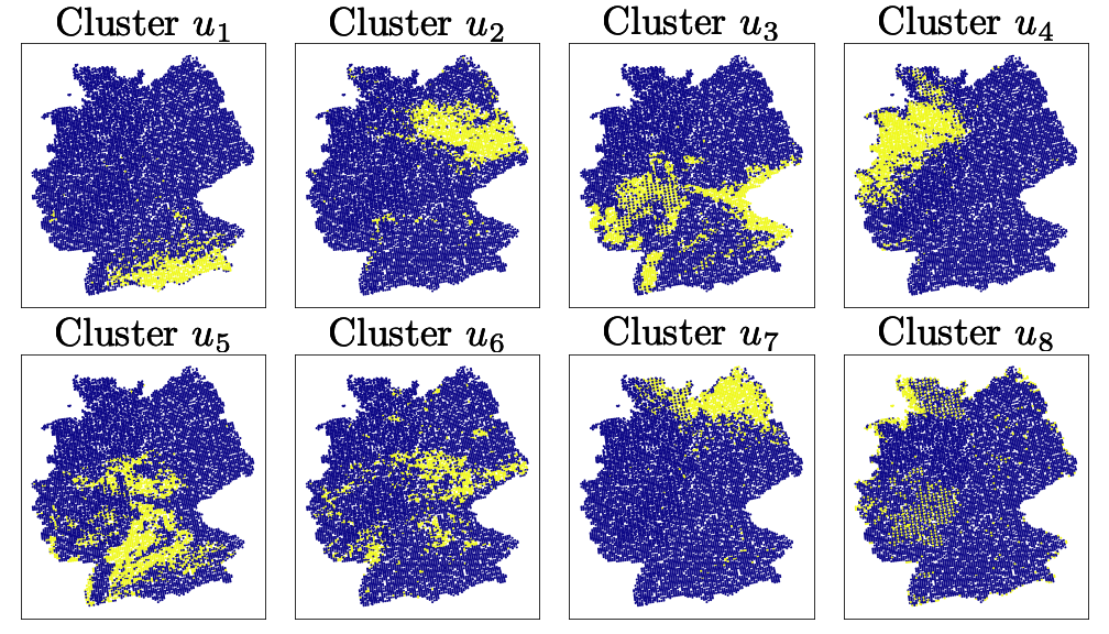
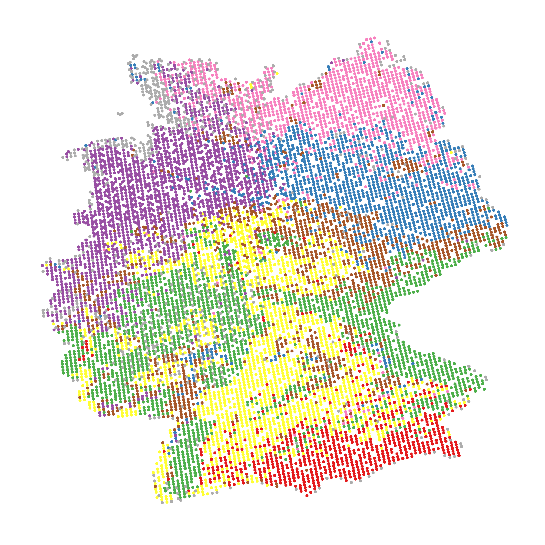
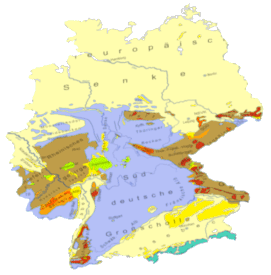
Figure 12 shows instance (region) clusters. A comparison with a geological map of Germany reveals that clusters correspond quite closely to distinct geological formations. Figure 13 shows the geographical distribution of sub-bags clusters (i.e., plants).

Figure 13: Visualization of the sub-bag clusters. Color is proportional to the number of species in each cluster.

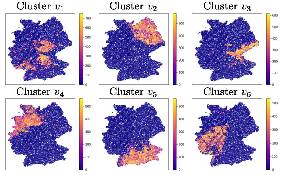
Instance to sub-bag and sub-bag to label rules are listed in Figures 14 and 15, respectively. Figure 14 illustrates some of the instance to sub-bag rules. Recall that each sub-bag (species) contains 25 instances (regions). Rule 1, for example, says that a sub-bag has cluster identifier $v_{1}$, if among these 25 regions there is at least one region in cluster $u_{5}$ (plotted in green), and none with in clusters $u_{1},u_{3},u_{4}$ (jointly plotted in red). Figure 15 illustrates sub-bag to label rules for the positive class. The top row corresponds to rules bodies (color proportional to the number of positive literals minus the number of negative literals); the bottom row shows regions that are classified as positive by each rule. The overall prediction is the union of these regions.

$1$	$v_{1}$	$\leftarrow$	$f_{u_{1}}=0,f_{u_{3}}=0,f_{u_{4}}=0,f_{u_{5}}=1.$
$2$	$v_{2}$	$\leftarrow$	$f_{u_{1}}=0,f_{u_{3}}=0,f_{u_{4}}=0,f_{u_{5}}=0.$
$3$	$v_{3}$	$\leftarrow$	$f_{u_{1}}=0,f_{u_{3}}=1,f_{u_{5}}=0,f_{u_{6}}=1.$
$4$	$v_{3}$	$\leftarrow$	$f_{u_{1}}=1,f_{u_{3}}=1,f_{u_{6}}=1,f_{u_{7}}=0.$
$5$	$v_{4}$	$\leftarrow$	$f_{u_{1}}=0,f_{u_{3}}=0,f_{u_{4}}=1,f_{u_{5}}=0.$
$6$	$v_{5}$	$\leftarrow$	$f_{u_{1}}=1,f_{u_{3}}=0.$
$7$	$v_{5}$	$\leftarrow$	$f_{u_{1}}=1,f_{u_{3}}=1,f_{u_{7}}=1.$
$8$	$v_{5}$	$\leftarrow$	$f_{u_{1}}=1,f_{u_{6}}=0.$
$9$	$v_{5}$	$\leftarrow$	$f_{u_{1}}=1,f_{u_{6}}=1,f_{u_{7}}=1.$
$10$	$v_{6}$	$\leftarrow$	$f_{u_{1}}=0,f_{u_{3}}=0,f_{u_{4}}=1,f_{u_{5}}=1.$
$11$	$v_{6}$	$\leftarrow$	$f_{u_{1}}=0,f_{u_{3}}=1,f_{u_{5}}=1,f_{u_{6}}=1.$
$12$	$v_{6}$	$\leftarrow$	$f_{u_{1}}=0,f_{u_{3}}=1,f_{u_{6}}=0.$

Figure 14: Top: Instance to sub-bag rules extracted from the MMIL network. Bottom: Visualization of instance to sub-bag rules $1$, $4$, $7$, $9$, and $11$.

$1$	$negative$	$\leftarrow$	$f_{v_{1}}=0,f_{v_{2}}=0,f_{v_{3}}=0.$
$2$	$negative$	$\leftarrow$	$f_{v_{1}}=0,f_{v_{2}}=0,f_{v_{4}}=0.$
$3$	$negative$	$\leftarrow$	$f_{v_{1}}=1,f_{v_{2}}=0,f_{v_{5}}=1,f_{v_{6}}=0.$
$4$	$negative$	$\leftarrow$	$f_{v_{1}}=1,f_{v_{2}}=0,f_{v_{6}}=1.$
$5$	$negative$	$\leftarrow$	$f_{v_{2}}=1,f_{v_{3}}=0,f_{v_{4}}=1,f_{v_{6}}=1.$
$6$	$positive$	$\leftarrow$	$f_{v_{2}}=1,f_{v_{4}}=0.$
$7$	$positive$	$\leftarrow$	$f_{v_{1}}=0,f_{v_{2}}=0,f_{v_{3}}=1,f_{v_{4}}=1.$
$8$	$positive$	$\leftarrow$	$f_{v_{1}}=1,f_{v_{2}}=0,f_{v_{5}}=0,f_{v_{6}}=0.$
$9$	$positive$	$\leftarrow$	$f_{v_{2}}=1,f_{v_{3}}=1,f_{v_{4}}=1.$
$10$	$positive$	$\leftarrow$	$f_{v_{2}}=1,f_{v_{4}}=1,f_{v_{6}}=0.$

Figure 15: Instance to sub-bag rules extracted from the MMIL network. Visualization of sub-bag to label rules for the positive class.

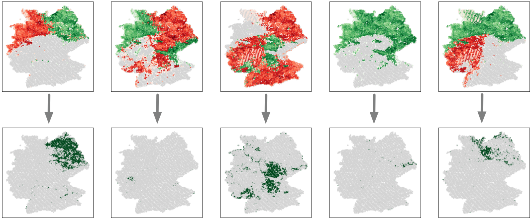
7 Conclusions

We have introduced the MMIL framework for handling data organized in nested bags. The MMIL setting allows for a natural hierarchical organization of data, where components at different levels of the hierarchy are unconstrained in their cardinality. We have identified several learning problems that can be naturally expressed as MMIL problems. For instance, image, text or graph classification are promising application areas, because here the examples can be objects of varying structure and size, for which a bag-of-bag data representation is quite suitable, and can provide a natural alternative to graph kernels or convolutional network for graphs. Furthermore we proposed new way of thinking in terms of interpretability. Although some MIL models can be easily interpreted by exploiting the learnt instance labels and the assumed rule, MMIL networks can be interpreted in a finer level: by removing the common assumptions of the standard MIL, we are more flexible and we can first associate labels to instances and sub-bags and then combine them in order to extract new rules. Finally, we proposed a different perspective to see convolutions on graphs. In most of the neural network for graphs approaches convolutions can be interpreted as message passing schema, while in our approach we provided a decomposition schema.

We proposed a neural network architecture involving the new construct of bag-layers for learning in the MMIL setting. Theoretical results show the expressivity of this type of model. In the empirical results we have shown that learning MMIL models from data is feasible, and the theoretical capabilities of MMIL networks can be exploited in practice, e.g., to learn accurate models for noiseless data. Furthermore MMIL networks can be applied in a wide spectrum of scenarios, such as text, image, and graphs. For this latter we showed that MMIL is competitive with the state-of-the-art models on node and graph classification tasks, and, in many cases, MMIL models outperform the others.

In this paper, we have focused on the setting where whole bags-of-bags are to be classified. In conventional MIL learning, it is also possible to define a task where individual instances are to be classified. Such a task is however less clearly defined in our setup since we do not assume to know the label spaces at the instance and sub-bag level, nor the functional relationship between the labels at the different levels.

Appendix A Details for the Experiments on Semi-Synthetic Data (Section 7.1)

Table 13: Neural network structure for MMIL MNIST dataset. The model was trained by minimizing the binary cross entropy loss. We ran 200 epochs of the Adam optimizer (Kingma and Ba, 2015) with learning rate 0.001 and mini-batch size of 20.

Layer	Parameters
Convolutional Layer	kernel size $5\times 5$ with 32 channels
Batch Normalization
ReLU
Max Pooling	kernel size $2\times 2$
Dropout	probability 0.5
Convolutional Layer	kernel size $5\times 5$ with 64 channels
Batch Normalization
ReLU
Max Pooling	kernel size $2\times 2$
Dropout	probability 0.5
Dense	$1024$ units
ReLU
Dropout	probability 0.5
BagLayer (ReLU activation)	$200$ units
ReLU
BagLayer (ReLU activation)	$200$ units
ReLU
Dense	$1$ unit

Figure 16: MNIST: Validation fidelity as a function of cluster sizes.

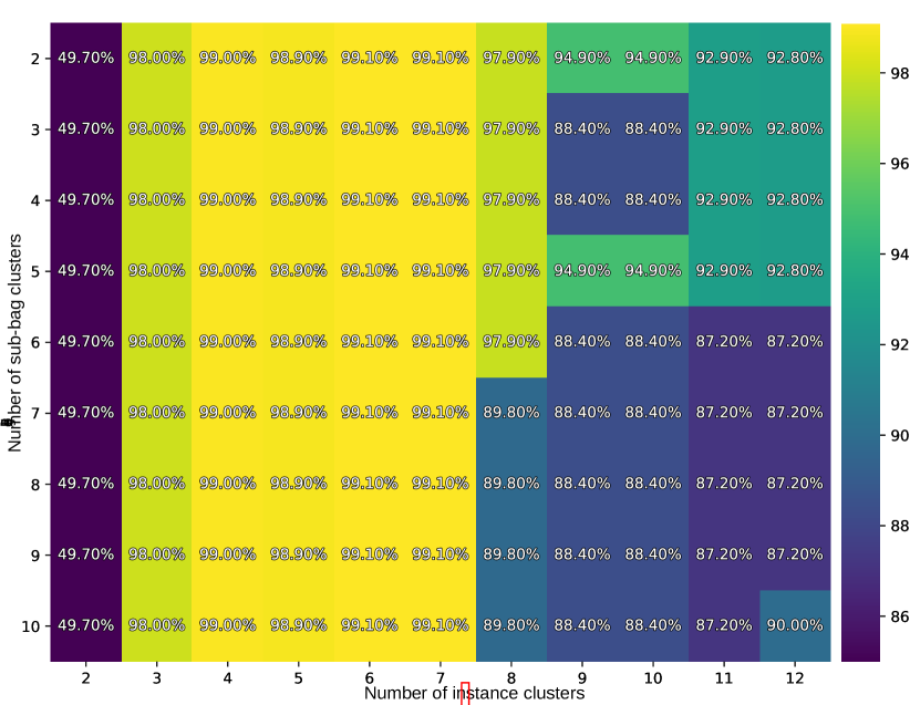
Appendix B Details for the Experiments on Sentiment Analysis (Section 6.2)

We report here a second example of classification explanation. Here we are considering a positive review that was misclassified as negative by the MMIL rules, and correctly classified by the MIL model. Following the same typesetting conventions as used in Table 7, the review and the labeling of the prediction-relevant parts are shown in Table 14. In the MMIL case, classification was due to rule 6 in Table 5. The sentence “The storyline is $\dots$” was assigned cluster identifier $v_{1}$ by rule 1 in Table 4, whereas the sentence “The mental patients$\dots$” was assigned cluster identifier $v_{3}$ by rule 6 in Table 4. The positive classification in the MIL case was due to rule 2 in Table 6, which is based on clusters $u_{3}$ and $u_{6}$.

Table 14: A sample positive review. Top: MMIL labeling. Bottom: MIL labeling.

Figure 17: IMDB: Validation fidelity as a function of cluster sizes.

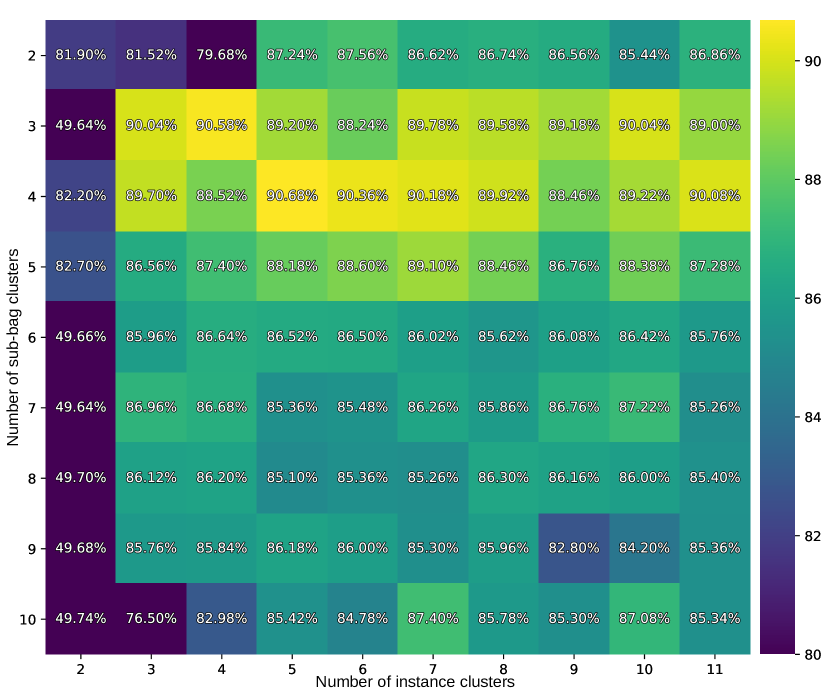
Appendix C Details for the Experiments on Citation Networks Data (Section 6.3)

Figure 18: Distribution of papers over years for Citaseer, Cora, and PubMed.

Figure 19: Pubmed: Validation fidelity as a function of cluster sizes.

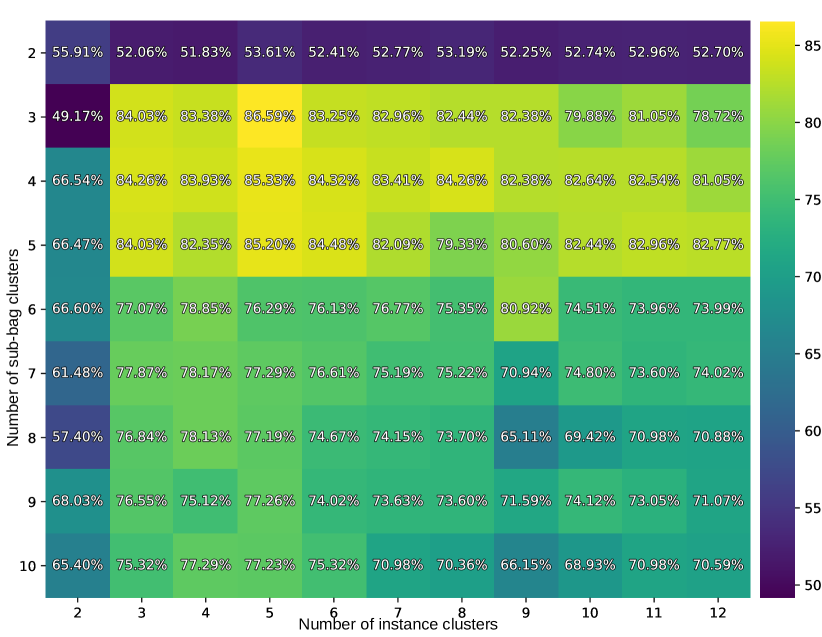
Here we interpret the MMIL-Mean and MIL-Mean models trained on the PubMed citation dataset (Section 6.3). In the MMIL setting, the optimal number of sub-bag and instance clusters in the validation set were three and five, respectively (see Figure 19). In the MIL setting the optimal number of instance clusters in the validation set was three.

Figure 20: Correspondence between sub-bag clusters and actual paper class labels.

Sub-bags in the MMIL decomposition also are papers, and therefore also are labeled with the actual class label. The number of inferred sub-bag clusters matches the true number of classes, and, as shown in Figure 20, clusters and classes strongly correlate. Instance (words) clusters are interpreted using the same approach as in Section 6.2. Result are shown in Table 19 for the MMIL setting and in Table 18 for the MIL setting.

Table 15: PubMed: MMIL rules for mapping instance cluster frequencies into a sub-bag cluster identifiers. See the caption of Table 4 for details on the syntax.

$$\begin{array}[]{ll}\hline\cr\hline\cr 1&v_{1}\leftarrow f_{u_{2}}\mathord{\leq}44.53,f_{u_{3}}\mathord{\leq}22.70,f_{u_{5}}\mathord{\leq}6.47.\\ 2&v_{1}\leftarrow f_{u_{2}}\mathord{\leq}44.53,f_{u_{3}}\mathord{\leq}31.31,f_{u_{5}}\mathord{>}6.47.\\ 3&v_{1}\leftarrow f_{u_{2}}\mathord{>}44.53,f_{u_{4}}\mathord{\leq}14.22,f_{u_{5}}\mathord{>}14.83.\\ 4&v_{2}\leftarrow f_{u_{2}}\mathord{>}44.53,f_{u_{3}}\mathord{\leq}22.60,f_{u_{4}}\mathord{>}14.22.\\ 5&v_{2}\leftarrow f_{u_{2}}\mathord{>}44.53,f_{u_{4}}\mathord{\leq}14.22,f_{u_{5}}\mathord{\leq}14.83.\\ 6&v_{3}\leftarrow f_{u_{2}}\mathord{\leq}44.53,f_{u_{3}}\mathord{>}22.70,f_{u_{5}}\mathord{\leq}6.47.\\ 7&v_{3}\leftarrow f_{u_{2}}\mathord{\leq}44.53,f_{u_{3}}\mathord{>}31.31,f_{u_{5}}\mathord{>}6.47.\\ 8&v_{3}\leftarrow f_{u_{2}}\mathord{>}44.53,f_{u_{3}}\mathord{>}22.60,f_{u_{4}}\mathord{>}14.22.\\ \hline\cr\hline\cr\end{array}$$

Rules extracted by our procedure are reported in Tables 15, 16 (MMIL) and 17 (MIL). Test set accuracies of the extracted rules were $76.88\%$ and $79.25\%$ in the MMIL and MIL setting, respectively. The corresponding fidelities were $84.75\%$ and $87.99\%$, respectively. Both of the results are still comparable and competitive with the methods described in Table 9. Thus, in this case the interpretable MIL model outperforms the interpretable MMIL model in terms of accuracy. However, for explaining individual classifications, the MMIL model can still have advantages due to the multi-level explanations it supports. As we did for the IMDB experiment (Section 6.2), one can first explain the predicted label of a paper in terms of the citing/cited papers assigned to the relevant clusters, and then refine this explanation by tracing paper cluster assignments to word clusters. In the MIL model, on the other hand, only word level explanations are possible.

Table 16: PubMed: MMIL rules mapping sub-bag cluster frequencies into top-bag labels. See the caption of Table 4 for details on the syntax.

$$\begin{array}[]{ll}\hline\cr\hline\cr 1&DME~{}\leftarrow f_{v_{1}}\mathord{\leq}8.51,f_{v_{2}}\mathord{>}63.96.\\ 2&DMT1\leftarrow f_{v_{1}}\in(8.51,20.26],f_{v_{2}}\mathord{>}63.96.\\ 3&DMT1\leftarrow f_{v_{1}}\mathord{>}20.26,f_{v_{3}}\mathord{\leq}55.49.\\ 4&DMT2\leftarrow f_{v_{1}}\mathord{\leq}20.26,f_{v_{2}}\mathord{\leq}63.96.\\ 5&DMT2\leftarrow f_{v_{1}}\mathord{>}20.26,f_{v_{3}}\mathord{>}55.49.\\ \hline\cr\hline\cr\end{array}$$

Table 17: PubMed: MIL classification rules. See the caption of Table 4 for details on the syntax.

$$\begin{array}[]{ll}\hline\cr\hline\cr 1&DME~{}\leftarrow f_{u_{1}}\mathord{>}49.80.\\ 2&DMT1\leftarrow f_{u_{1}}\mathord{\leq}49.80,f_{u_{2}}\mathord{\leq}30.60,f_{u_{3}}\mathord{\leq}30.65.\\ 3&DMT1\leftarrow f_{u_{1}}\mathord{\leq}49.80,f_{u_{2}}\mathord{>}30.60,f_{u_{3}}\mathord{\leq}35.66.\\ 4&DMT1\leftarrow f_{u_{1}}\mathord{\leq}49.80,f_{u_{2}}\mathord{\leq}30.60,f_{u_{3}}\mathord{>}30.65.\\ 5&DMT1\leftarrow f_{u_{1}}\mathord{\leq}49.80,f_{u_{2}}\mathord{>}30.60,f_{u_{3}}\mathord{>}35.66.\\ \hline\cr\hline\cr\end{array}$$

Table 18: PubMed: Clusters in the MIL case. Each column represents words belonging to the associated cluster. The percentage next to each cluster identifier refers to the number of of words associated with that cluster ($\approx 15$k). Words are ranked by intra-cluster distance in descending order.

$u_{1}$ $(48.33\%)$	$u_{2}$ $(60.09\%)$	$u_{3}$ $(41.92\%)$
animals	children	non
induction	juvenile	subjects
induced	multiplex	patients
experimental	hla	indians
rats	childhood	fasting
rat	adolescents	obesity
dogs	conventional	pima
caused	girls	american
days	ascertainment	mexican
strains	autoimmune	indian
bl	dr	mody
experiment	infusion	oral
untreated	child	bmi
wk	siblings	obese
sz	intensive	men
restored	healthy	prevalence
sciatic	paediatric	resistance
experimentally	spk	tolerance
sprague	boys	mutations
partially	sharing	igt

Table 19: PubMed: Clusters in the MMIL case. Each column represents words belonging to the associated cluster. The percentage next to the cluster identifier refers to the number of of words associated with that cluster ($\approx 15$k). Words in cluster $u_{1}$ are grayed out since that cluster is never used for constructing the rules. Words are ranked by intra-cluster distance in descending order.

$u_{1}$ $(21.28\%)$	$u_{2}$ $(28.76\%)$	$u_{3}$ $(27.25\%)$	$u_{4}$ $(12.84\%)$	$u_{5}$ $(9.87\%)$
normalization	animals	non	subjects	children
greatly	experimental	indians	patients	multiplex
susceptibility	induced	pima	patient	ascertainment
lymphocytes	induction	obesity	individuals	conventional
pregnant	rats	oral	type	juvenile
always	dogs	fasting	analysis	girls
organ	made	mexican	sample	night
destruction	rat	obese	cascade	childhood
tx	strains	medication	otsuka	pittsburgh
contraction	bl	bmi	forearm	adolescents
antibodies	caused	mody	gdr	infusion
sequential	wk	indian	reported	denmark
tract	counteracted	tolerance	mmol	intensified
decarboxylase	partially	look	age	child
recipients	rabbits	index	gox	beef
livers	days	agents	dependent	sharing
mt	conscious	resistance	isoforms	knowing
cyclosporin	sciatic	maturity	meals	paediatric
lv	tubules	gk	score	unawareness
laboratories	myo	ii	affinities	pubert

Appendix D Details for the Experiments on Point Clouds (Section 6.5)

Like in Section 6.1, we derived interpreting rules in the MMIL setting on the P100 dataset. Using 2,000 point clouds as a validation set, we obtained 47 and 42 clusters for sub-bags and instances, respectively. For the rules mapping instance cluster identifiers to subbag cluster identifiers the decision tree was used as propositional learner (as the aggregation function in the first Bag-Layer is the $\max$), while for the rules mapping subbag cluster identifiers to topbag labels the decision tree considered the counts of subbag identifiers (as the aggregation function in the second Bag-Layer is the sum). Full grid search results on the validation set are reported in Figure 21. Accuracy using rules was $59.12\%$, corresponding to a fidelity of $61.83\%$.

Figure 21: PointCloud: Validation fidelity as a function of cluster sizes.

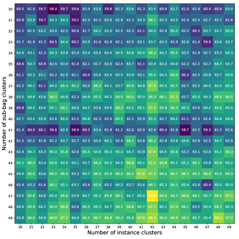
Some examples are shown in Figure 22. Subbag cluster identifiers (see Table 20) $v_{5}$, $v_{31}$, $v_{4}$ correspond to airplane, the guitar and the table, respectively. The blue points represent the original point clouds. For readability, in Figure 22 we only distinguish between regions with active (green) and inactive (red) instance clusters in the rules of Table 20.

Figure 22: Three point clouds examples. The green and red boxes represents the active and inactive regions, respectively for the corresponding clusters.

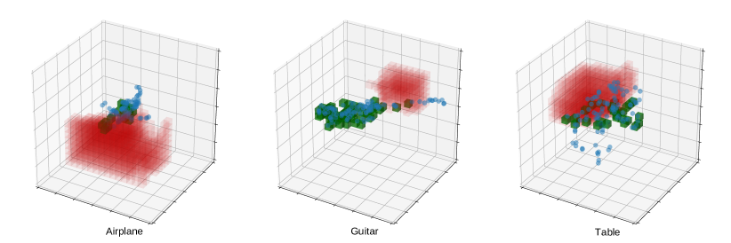
MMIL rules.

Using a decision tree learner taking binary vectors $(f_{u_{1}},\ldots,f_{u_{42}})$ as inputs, we obtained 959 rules for mapping a bag $x_{j}$ of instance cluster identifiers to a sub-bag cluster identifiers and 85 rules for mapping sub-bag cluster identifiers to the top-bag class labels. We do not report the full sets of rules here. However we report in Table 20 the rules corresponding to the three point clouds depicted in Figure 22. In particular $v_{5}$, $v_{31}$ and $v_{4}$ are the sub-bag clusters associated with classes airplane, guitar, and table, respectively.

Table 20: Rules extracted from the MMIL network for mapping instance cluster identifiers into a sub-bag cluster identifiers.

$1$	$v_{5}$	$\leftarrow$	$f_{u_{9}}=1,\ f_{u_{13}}=1,\ f_{u_{14}}=1,\ f_{u_{18}}=1,\ f_{u_{15}}=0,$
			$f_{u_{16}}=0,\ f_{u_{21}}=0,\ f_{u_{35}}=0,\ f_{u_{39}}=0,\ f_{u_{41}}=0.$
$2$	$v_{31}$	$\leftarrow$	$f_{u_{13}}=1,\ f_{u_{15}}=1,f_{u_{32}}=1,\ f_{u_{33}}=1,f_{u_{4}}=0,$
			$f_{u_{5}}=1,\ f_{u_{9}}=0,\ f_{u_{18}}=0,\ f_{u_{31}}=0.$
$3$	$v_{4}$	$\leftarrow$	$f_{u_{12}}=1,\ f_{u_{13}}=1,\ f_{u_{15}}=1,\ f_{u_{41}}=1,\ f_{u_{30}}=1,$
			$f_{u_{31}}=0,\ f_{u_{32}}=0,\ f_{u_{35}}=1,\ f_{u_{37}}=0.$

For the left example (airplane) in Figure 22, all subbags are in cluster $v_{5}$. For the middle example (guitar) two subbag are in $v_{31}$ and three in $v_{24}$. For the right example (table) all subbags are in $v_{4}$. By inspecting Figure 23 we can have an immediate intuition for the predicted topbag labels. In fact, $v_{5}$ exclusively correlates with airplanes, $v_{31}$ correlates mainly with keyboards and sometimes with guitars, $v_{24}$ correlates most exclusively with guitars, and $v_{4}$ correlates most exclusively with desks. We would then expect that the left and middle examples are correctly classified as airplane and guitar, respectively, while the right example is misclassified as desk (the correct label was table). Finally, Table 21 shows the rules (which confirm the intuition) that connects the subbag cluster identifiers to topbag labels for the examples depicted in Figure 22.

Table 21: Rules extracted from the MMIL network for mapping subbag cluster identifiers into the top-bag label.

$1$	$l_{airplane}$	$\leftarrow$	$f_{v_{5}}>3,f_{v_{2}}\leq 1,f_{v_{16}}\leq 2.$
$2$	$l_{guitar}$	$\leftarrow$	$f_{v_{24}}>2,f_{v_{2}}\leq 1,f_{v_{3}}\leq 1,f_{v_{5}}\leq 2,f_{v_{9}}\leq 1,f_{v_{x10}}\leq 1,f_{v_{11}}\leq 1,f_{v_{13}}\leq 1,f_{v_{15}}\leq 2,$
			$f_{v_{16}}\leq 2,f_{v_{17}}\leq 3,f_{v_{18}}\leq 1,f_{v_{8}}=0,f_{v_{23}}=0,f_{v_{25}}=0,f_{v_{28}}=0,f_{v_{37}}=0.$
$3$	$l_{desk}$	$\leftarrow$	$f_{v_{4}}>1,f_{v_{2}}\leq 1,f_{v_{3}}\leq 1,f_{v_{5}}\leq 2,f_{v_{9}}\leq 1,f_{v_{11}}\leq 1,f_{v_{13}}\leq 1,f_{v_{14}}\leq 1,$
			$f_{v_{15}}\leq 2,f_{v_{16}}\leq 1,f_{v_{17}}\leq 3,f_{v_{18}}\leq 1,f_{v_{20}}\leq 2,f_{v_{22}}\leq 2,f_{v_{24}}\leq 1,f_{v_{28}}\leq 1,$
			$f_{v_{30}}\leq 1,f_{v_{36}}\leq 2,f_{v_{8}}=0,f_{v_{10}}=0,f_{v_{23}}=0,f_{v_{25}}=0,f_{v_{29}}=0,f_{v_{37}}=0.$

Figure 23: Correspondence between subbag cluster identifiers and actual point cloud class labels. Class labels without correspondence are omitted.

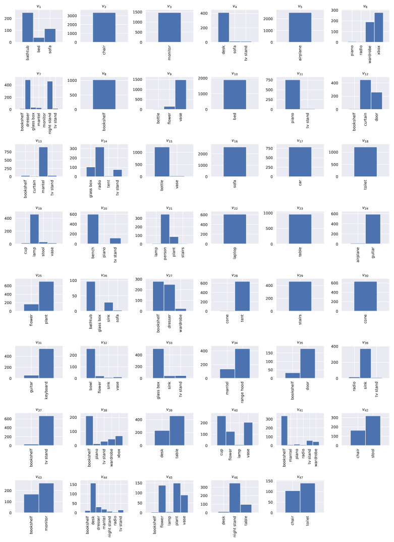
Appendix E Notation

Table 22: Notation

Symbol	Description
$\mathcal{M}(A)$	set of multisets of elements from $A$
$x$	top-bag
$x_{j}$	sub-bag
$x_{{j},{\ell}}$	is a instance
$n$	cardinality of top-bag $x$
$n_{j}$	cardinality of sub-bag $x_{j}$
$\mathcal{X}$	instance space
$\mathcal{Y}^{\mathrm{inst}}$	instance label space
$\mathcal{Y}^{\mathrm{sub}}$	sub-bag label space
$\mathcal{Y}$	the top-bag label space
$y_{j,\ell}$	label associated with $x_{{j},{\ell}}$
$y_{j}$	label associated with $x_{j}$.
$y$	label associated with $x$
$g$	is the bag-layer function
$F$	is the MMIL network
$\mathcal{C}^{\mathrm{inst}}$	approximated instance label space
$\mathcal{C}^{\mathrm{sub}}$	approximated sub-bag label space
$k^{\mathrm{inst}}$	cardinality of $\mathcal{C}^{\mathrm{inst}}$
$k^{\mathrm{sub}}$	is the cardinality of $\mathcal{C}^{\mathrm{sub}}$
$I$	multi-set of the instance representations
$S$	multi-set of the sub-bag representations
$r$	function mapping elements in $\mathcal{X}$ to elements in $\mathcal{C}^{\mathrm{inst}}$
$s$	function mapping elements in $\mathcal{C}^{\mathrm{inst}}$ to elements in $\mathcal{C}^{\mathrm{sub}}$
$t$	function mapping elements in $\mathcal{C}^{\mathrm{sub}}$ to elements in $\mathcal{Y}^{\mathrm{inst}}$
$\phi_{j}$	feature representation corresponding to $x_{j}$
$\phi$	feature representation corresponding to $x$
$\rho_{i}$	activation of the $i$-th node of the bag-layer before performing the aggregation

References

- [1] Flora von deutschland (phanerogamen). URL https://doi.org/10.15468/0fxsox. GBIF Occurrence Download https://doi.org/10.15468/dl.gj34x1.
- Andrews et al. [2002] Stuart Andrews, Ioannis Tsochantaridis, and Thomas Hofmann. Support vector machines for multiple-instance learning. In Advances in neural information processing systems, pages 561–568, 2002.
- Arbelaez et al. [2011] Pablo Arbelaez, Michael Maire, Charless Fowlkes, and Jitendra Malik. Contour Detection and Hierarchical Image Segmentation. IEEE Transactions on Pattern Analysis and Machine Intelligence, 33(5):898–916, May 2011. doi: 10.1109/TPAMI.2010.161.
- Arora et al. [2016] Sanjeev Arora, Yingyu Liang, and Tengyu Ma. A simple but tough-to-beat baseline for sentence embeddings. In International Conference on Learning Representations (ICLR), 2016.
- Atwood and Towsley [2016] James Atwood and Don Towsley. Diffusion-convolutional neural networks. In Advances in Neural Information Processing Systems, pages 1993–2001, 2016.
- Bach et al. [2015] Sebastian Bach, Alexander Binder, Grégoire Montavon, Frederick Klauschen, Klaus-Robert Müller, and Wojciech Samek. On pixel-wise explanations for non-linear classifier decisions by layer-wise relevance propagation. PloS one, 10(7), 2015.
- Blei et al. [2003] David M. Blei, Andrew Y. Ng, and Michael I. Jordan. Latent dirichlet allocation. Journal of Machine Learning Research, 3:993–1022, 2003. URL http://dl.acm.org/citation.cfm?id=944937.
- Costa and De Grave [2010] Fabrizio Costa and Kurt De Grave. Fast neighborhood subgraph pairwise distance kernel. In Proceedings of the 26th International Conference on Machine Learning, pages 255–262. Omnipress, 2010.
- De Raedt et al. [2008a] L. De Raedt, B. Demoen, D. Fierens, B. Gutmann, G. Janssens, A. Kimmig, N. Landwehr, T. Mantadelis, W. Meert, R. Rocha, et al. Towards digesting the alphabet-soup of statistical relational learning, 2008a.
- De Raedt et al. [2008b] Luc De Raedt, Paolo Frasconi, Kristian Kersting, and Stephen Muggleton. Probabilistic inductive logic programming: theory and applications, 2008b.
- Dietterich [2000] Thomas G. Dietterich. Ensemble Methods in Machine Learning. In Multiple Classifier Systems, number 1857 in Lecture Notes in Computer Science, pages 1–15. Springer Berlin Heidelberg, June 2000. ISBN 978-3-540-67704-8 978-3-540-45014-6.
- Dietterich et al. [1997] Thomas G. Dietterich, Richard H. Lathrop, and Tomás Lozano-Pérez. Solving the multiple instance problem with axis-parallel rectangles. Artificial Intelligence, 89(1–2):31–71, January 1997. doi: 10.1016/S0004-3702(96)00034-3.
- Duvenaud et al. [2015] David K Duvenaud, Dougal Maclaurin, Jorge Iparraguirre, Rafael Bombarell, Timothy Hirzel, Alán Aspuru-Guzik, and Ryan P Adams. Convolutional networks on graphs for learning molecular fingerprints. In Advances in neural information processing systems, pages 2224–2232, 2015.
- Foulds and Frank [2010] James Foulds and Eibe Frank. A review of multi-instance learning assumptions. The Knowledge Engineering Review, 25(01):1, March 2010. doi: 10.1017/S026988890999035X.
- Frasconi et al. [1998] P. Frasconi, M. Gori, and A. Sperduti. A general framework for adaptive processing of data structures. IEEE Trans. on Neural Networks, 9:768–786, 1998.
- Fukushima [1980] Kunihiko Fukushima. Neocognitron: A self-organizing neural network model for a mechanism of pattern recognition unaffected by shift in position. Biological cybernetics, 36(4):193–202, 1980.
- Gardner et al. [2018] Jacob R Gardner, Geoff Pleiss, David Bindel, Kilian Q Weinberger, and Andrew Gordon Wilson. Gpytorch: Blackbox matrix-matrix gaussian process inference with gpu acceleration. In Advances in Neural Information Processing Systems, 2018.
- Gärtner et al. [2004] Thomas Gärtner, John W Lloyd, and Peter A Flach. Kernels and distances for structured data. Machine Learning, 57(3):205–232, 2004.
- Getoor and Taskar [2007] Lise Getoor and Ben Taskar. Introduction to statistical relational learning. MIT Press, Cambridge, Mass., 2007.
- Gilmer et al. [2017] Justin Gilmer, Samuel S. Schoenholz, Patrick F. Riley, Oriol Vinyals, and George E. Dahl. Neural message passing for quantum chemistry. In Proceedings of the 34th International Conference on Machine Learning, ICML 2017, pages 1263–1272, 2017. URL http://proceedings.mlr.press/v70/gilmer17a.html.
- Gori et al. [2005] Marco Gori, Gabriele Monfardini, and Franco Scarselli. A new model for learning in graph domains. In Neural Networks, 2005. IJCNN’05. Proceedings. 2005 IEEE International Joint Conference on, volume 2, pages 729–734. IEEE, 2005.
- Griffiths and Steyvers [2004] Thomas L Griffiths and Mark Steyvers. Finding scientific topics. Proceedings of the National academy of Sciences, 101(suppl 1):5228–5235, 2004.
- Hamilton et al. [2017] Will Hamilton, Zhitao Ying, and Jure Leskovec. Inductive representation learning on large graphs. In Advances in Neural Information Processing Systems, pages 1024–1034, 2017.
- Haussler [1999] David Haussler. Convolution kernels on discrete structures. Technical Report 646, Department of Computer Science, University of California at Santa Cruz, 1999.
- Hensman et al. [2015] James Hensman, Alexander Matthews, and Zoubin Ghahramani. Scalable variational gaussian process classification. 2015.
- Hentschel and Sack [2015] Christian Hentschel and Harald Sack. What image classifiers really see–visualizing bag-of-visual words models. In International Conference on Multimedia Modeling, pages 95–104. Springer, 2015.
- Horváth et al. [2004] Tamás Horváth, Thomas Gärtner, and Stefan Wrobel. Cyclic pattern kernels for predictive graph mining. In Proceedings of the tenth ACM SIGKDD international conference on Knowledge discovery and data mining, pages 158–167. ACM, 2004.
- Hou et al. [2015] Le Hou, Dimitris Samaras, Tahsin M Kurc, Yi Gao, James E Davis, and Joel H Saltz. Efficient multiple instance convolutional neural networks for gigapixel resolution image classification. arXiv preprint arXiv:1504.07947, 2015.
- Jaeger [1997] M. Jaeger. Relational bayesian networks. In Dan Geiger and Prakash Pundalik Shenoy, editors, Proceedings of the 13th Conference of Uncertainty in Artificial Intelligence (UAI-13), pages 266–273, Providence, USA, 1997. Morgan Kaufmann.
- Kingma and Ba [2015] Diederik Kingma and Jimmy Ba. Adam: A Method for Stochastic Optimization. In 3rd International Conference for Learning Representations, San Diego, CA, 2015. arXiv:1412.6980.
- Kipf and Welling [2016] Thomas N. Kipf and Max Welling. Semi-supervised classification with graph convolutional networks. arXiv preprint arXiv:1609.02907, 2016.
- Kondor and Jebara [2003] Risi Kondor and Tony Jebara. A kernel between sets of vectors. In Machine Learning, Proceedings of the Twentieth International Conference (ICML 2003), August 21-24, 2003, Washington, DC, USA, pages 361–368, 2003. URL http://www.aaai.org/Library/ICML/2003/icml03-049.php.
- Landwehr et al. [2010] N. Landwehr, A. Passerini, L. De Raedt, and P. Frasconi. Fast learning of relational kernels. Machine learning, 78(3):305–342, 2010.
- Lapuschkin et al. [2016] Sebastian Lapuschkin, Alexander Binder, Grégoire Montavon, Klaus-Robert Müller, and Wojciech Samek. The lrp toolbox for artificial neural networks. The Journal of Machine Learning Research, 17(1):3938–3942, 2016.
- LeCun et al. [1989] Yann LeCun, Bernhard Boser, John S. Denker, Donnie Henderson, Richard E. Howard, Wayne Hubbard, and Lawrence D. Jackel. Backpropagation applied to handwritten zip code recognition. Neural computation, 1(4):541–551, 1989.
- Lusci et al. [2013] Alessandro Lusci, Gianluca Pollastri, and Pierre Baldi. Deep architectures and deep learning in chemoinformatics: The prediction of aqueous solubility for drug-like molecules. Journal of Chemical Information and Modeling, 53(7):1563–1575, Jul 2013. ISSN 1549-960X. doi: 10.1021/ci400187y. URL http://dx.doi.org/10.1021/ci400187y.
- Maas et al. [2011] Andrew L. Maas, Raymond E. Daly, Peter T. Pham, Dan Huang, Andrew Y. Ng, and Christopher Potts. Learning word vectors for sentiment analysis. In Proceedings of the 49th Annual Meeting of the Association for Computational Linguistics: Human Language Technologies, pages 142–150, Portland, Oregon, USA, June 2011. Association for Computational Linguistics.
- Maron and Lozano-Pérez [1998] Oded Maron and Tomás Lozano-Pérez. A framework for multiple-instance learning. Advances in neural information processing systems, pages 570–576, 1998.
- Maron and Ratan [1998] Oded Maron and Aparna Lakshmi Ratan. Multiple-instance learning for natural scene classification. In ICML, volume 98, pages 341–349, 1998.
- Minsky and Papert [1988] Marvin Minsky and Seymour A. Papert. Perceptrons, expanded edition. The MIT Press, 1988.
- Miyato et al. [2016] Takeru Miyato, Andrew M Dai, and Ian Goodfellow. Virtual adversarial training for semi-supervised text classification. In International Conference on Learning Representations (ICLR), 2016.
- Natarajan et al. [2008] Sriraam Natarajan, Prasad Tadepalli, Thomas G. Dietterich, and Alan Fern. Learning first-order probabilistic models with combining rules. Annals of Mathematics and Artificial Intelligence, 54(1-3):223–256, 2008. URL http://link.springer.com/article/10.1007/s10472-009-9138-5.
- Neumann et al. [2012] Marion Neumann, Novi Patricia, Roman Garnett, and Kristian Kersting. Efficient graph kernels by randomization. In Joint European Conference on Machine Learning and Knowledge Discovery in Databases, pages 378–393. Springer, 2012. URL http://link.springer.com/chapter/10.1007/978-3-642-33460-3_30.
- Niepert et al. [2016] Mathias Niepert, Mohamed Ahmed, and Konstantin Kutzkov. Learning Convolutional Neural Networks for Graphs. In International conference on machine learning, pages 2014–2023, 2016.
- Oliver and Webster [1990] Margaret A Oliver and Richard Webster. Kriging: a method of interpolation for geographical information systems. International Journal of Geographical Information System, 4(3):313–332, 1990.
- Orsini et al. [2015] Francesco Orsini, Paolo Frasconi, and Luc De Raedt. Graph invariant kernels. In Proceedings of the Twenty-fourth International Joint Conference on Artificial Intelligence, pages 3756–3762, 2015.
- Orsini et al. [2018] Francesco Orsini, Daniele Baracchi, and Paolo Frasconi. Shift aggregate extract networks. Frontiers in Robotics and AI, 5:42, 2018.
- Passerini et al. [2006] Andrea Passerini, Paolo Frasconi, and Luc De Raedt. Kernels on prolog proof trees: Statistical learning in the ilp setting. Journal of Machine Learning Research, 7(Feb):307–342, 2006.
- Pennington et al. [2014] Jeffrey Pennington, Richard Socher, and Christopher D. Manning. Glove: Global vectors for word representation. In Empirical Methods in Natural Language Processing (EMNLP), pages 1532–1543, 2014.
- Rahmani et al. [2005] Rouhollah Rahmani, Sally A Goldman, Hui Zhang, John Krettek, and Jason E Fritts. Localized content based image retrieval. In Proceedings of the 7th ACM SIGMM international workshop on Multimedia information retrieval, pages 227–236. ACM, 2005.
- Ramon and De Raedt [2000] Jan Ramon and Luc De Raedt. Multi instance neural networks. In Proceedings of the ICML-2000 workshop on attribute-value and relational learning, 2000.
- Ribeiro et al. [2016] Marco Tulio Ribeiro, Sameer Singh, and Carlos Guestrin. Why should i trust you?: Explaining the predictions of any classifier. In Proceedings of the 22nd ACM SIGKDD international conference on knowledge discovery and data mining, pages 1135–1144. ACM, 2016.
- Richardson and Domingos [2006] Matthew Richardson and Pedro Domingos. Markov logic networks. Machine Learning, 62:107–136, 2006.
- Rusu and Cousins [2011] Radu Bogdan Rusu and Steve Cousins. 3d is here: Point cloud library (pcl). In 2011 IEEE international conference on robotics and automation, pages 1–4. IEEE, 2011.
- Samek et al. [2016] Wojciech Samek, Grégoire Montavon, Alexander Binder, Sebastian Lapuschkin, and Klaus-Robert Müller. Interpreting the predictions of complex ml models by layer-wise relevance propagation. In NIPS 2016 Workshop on Interpretable Machine Learning in Complex Systems, 2016. arXiv:1611.08191.
- Scarselli et al. [2009] Franco Scarselli, Marco Gori, Ah Chung Tsoi, Markus Hagenbuchner, and Gabriele Monfardini. The graph neural network model. IEEE Transactions on Neural Networks, 20(1):61–80, 2009.
- Sen et al. [2008] Prithviraj Sen, Galileo Namata, Mustafa Bilgic, Lise Getoor, Brian Galligher, and Tina Eliassi-Rad. Collective classification in network data. AI magazine, 29(3):93, 2008.
- Shawe-Taylor [1989] J. Shawe-Taylor. Building symmetries into feedforward networks. In First IEEE International Conference on Artificial Neural Networks, (Conf. Publ. No. 313), pages 158–162, 1989.
- Shervashidze et al. [2009] Nino Shervashidze, S. V. N. Vishwanathan, Tobias Petri, Kurt Mehlhorn, and Karsten M. Borgwardt. Efficient graphlet kernels for large graph comparison. In AISTATS, volume 5, pages 488–495, 2009.
- Shervashidze et al. [2011] Nino Shervashidze, Pascal Schweitzer, Erik Jan Van Leeuwen, Kurt Mehlhorn, and Karsten M. Borgwardt. Weisfeiler-lehman graph kernels. The Journal of Machine Learning Research, 12:2539–2561, 2011.
- Szegedy et al. [2017] Christian Szegedy, Sergey Ioffe, Vincent Vanhoucke, and Alex Alemi. Inception-v4, Inception-ResNet and the Impact of Residual Connections on Learning. In Proc. of AAAI, 2017. arXiv: 1602.07261.
- Tibo et al. [2017] Alessandro Tibo, Paolo Frasconi, and Manfred Jaeger. A network architecture for multi-multi-instance learning. In Joint European Conference on Machine Learning and Knowledge Discovery in Databases, pages 737–752. Springer, 2017.
- Uijlings et al. [2012] Jasper RR Uijlings, Arnold WM Smeulders, and Remko JH Scha. The visual extent of an object. International journal of computer vision, 96(1):46–63, 2012.
- Velickovic et al. [2018] Petar Velickovic, Guillem Cucurull, Arantxa Casanova, Adriana Romero, Pietro Liò, and Yoshua Bengio. Graph attention networks. In 6th International Conference on Learning Representations, ICLR, 2018. URL https://openreview.net/forum?id=rJXMpikCZ.
- Verstrepen et al. [2017] Koen Verstrepen, Kanishka Bhaduriy, Boris Cule, and Bart Goethals. Collaborative filtering for binary, positiveonly data. ACM SIGKDD Explorations Newsletter, 19(1):1–21, 2017.
- Vinyals et al. [2016] Oriol Vinyals, Samy Bengio, and Manjunath Kudlur. Order matters: Sequence to sequence for sets. In 4th International Conference on Learning Representations, ICLR 2016, 2016. URL http://arxiv.org/abs/1511.06391.
- Wang and Zucker [2000] Jun Wang and Jean-Daniel Zucker. Solving multiple-instance problem: A lazy learning approach. In Proceedings of the Seventeenth International Conference on Machine Learning, 2000.
- Williams and Rasmussen [2006] Christopher KI Williams and Carl Edward Rasmussen. Gaussian processes for machine learning, volume 2. MIT press Cambridge, MA, 2006.
- Wu et al. [2015] Zhirong Wu, Shuran Song, Aditya Khosla, Fisher Yu, Linguang Zhang, Xiaoou Tang, and Jianxiong Xiao. 3d shapenets: A deep representation for volumetric shapes. In Proceedings of the IEEE conference on computer vision and pattern recognition, pages 1912–1920, 2015.
- Yan et al. [2016] Zhennan Yan, Yiqiang Zhan, Zhigang Peng, Shu Liao, Yoshihisa Shinagawa, Shaoting Zhang, Dimitris N Metaxas, and Xiang Sean Zhou. Multi-instance deep learning: Discover discriminative local anatomies for bodypart recognition. IEEE transactions on medical imaging, 35(5):1332–1343, 2016.
- Yanardag and Vishwanathan [2015] Pinar Yanardag and SVN Vishwanathan. Deep graph kernels. In Proceedings of the 21th ACM SIGKDD International Conference on Knowledge Discovery and Data Mining, pages 1365–1374. ACM, 2015.
- Yang et al. [2006] Changbo Yang, Ming Dong, and Jing Hua. Region-based image annotation using asymmetrical support vector machine-based multiple-instance learning. In Computer Vision and Pattern Recognition, 2006 IEEE Computer Society Conference on, volume 2, pages 2057–2063. IEEE, 2006.
- Yang and Lozano-Perez [2000] Cheng Yang and Tomas Lozano-Perez. Image database retrieval with multiple-instance learning techniques. In Data Engineering, 2000. Proceedings. 16th International Conference on, pages 233–243. IEEE, 2000.
- Zaheer et al. [2017] Manzil Zaheer, Satwik Kottur, Siamak Ravanbakhsh, Barnabas Poczos, Russ R Salakhutdinov, and Alexander J Smola. Deep sets. In Advances in neural information processing systems, pages 3391–3401, 2017.
- Zha et al. [2008] Zheng-Jun Zha, Xian-Sheng Hua, Tao Mei, Jingdong Wang, Guo-Jun Qi, and Zengfu Wang. Joint multi-label multi-instance learning for image classification. In Computer Vision and Pattern Recognition, 2008. CVPR 2008. IEEE Conference on, pages 1–8. IEEE, 2008.
- Zhou et al. [2008] Yunhong Zhou, Dennis Wilkinson, Robert Schreiber, and Rong Pan. Large-scale parallel collaborative filtering for the netflix prize. In International conference on algorithmic applications in management, pages 337–348. Springer, 2008.
- Zhou et al. [2005] Zhi-Hua Zhou, Kai Jiang, and Ming Li. Multi-instance learning based Web mining. Applied Intelligence, 22(2):135–147, 2005.
- Zhou et al. [2012] Zhi-Hua Zhou, Min-Ling Zhang, Sheng-Jun Huang, and Yu-Feng Li. Multi-instance multi-label learning. Artificial Intelligence, 176(1):2291–2320, January 2012. doi: 10.1016/j.artint.2011.10.002.