AutoParallel: A Python module for automatic parallelization
and distributed execution of affine loop nests

Abstract

The last improvements in programming languages, programming models, and frameworks have focused on abstracting the users from many programming issues. Among others, recent programming frameworks include simpler syntax, automatic memory management and garbage collection, which simplifies code re-usage through library packages, and easily configurable tools for deployment. For instance, Python has risen to the top of the list of the programming languages [1] due to the simplicity of its syntax, while still achieving a good performance even being an interpreted language. Moreover, the community has helped to develop a large number of libraries and modules, tuning them to obtain great performance.

However, there is still room for improvement when preventing users from dealing directly with distributed and parallel computing issues. This paper proposes and evaluates AutoParallel, a Python module to automatically find an appropriate task-based parallelization of affine loop nests to execute them in parallel in a distributed computing infrastructure. This parallelization can also include the building of data blocks to increase task granularity in order to achieve a good execution performance. Moreover, AutoParallel is based on sequential programming and only contains a small annotation in the form of a Python decorator so that anyone with little programming skills can scale up an application to hundreds of cores.

1 Introduction

Computer simulations have become more and more crucial to both theoretical and experimental studies in many different fields, such as structural mechanics, chemistry, biology, genetics, and even sociology. Several years ago, small simulations (with up to several cores or even several nodes within the same grid) were enough to fulfill the scientific community requirements and thus, the experts of each field were capable of programming and running them. However, nowadays, simulations requiring hundreds or thousands of cores are widely used and, to this point, efficiently programming them becomes a challenge even for computer scientists. On the one hand, interdisciplinary teams have become popular, with field experts and computer scientists joining their forces together to keep their research at the forefront. On the other hand, programming languages have made a considerable effort to ease the programmability while maintaining acceptable performance. In this sense, Python [2] has risen to the top language for nonexperts [1], being easy to program while maintaining good performance trade-off and having a large number of third-party libraries available. Similarly, Go [3] has also gained some momentum thanks to its portability, reliability, and ease of concurrent programming, although it is still in its early stages.

Even if some great efforts have been accomplished for programming frameworks to ease the development of distributed applications, we go one step further with AutoParallel: a Python module to automatically parallelize applications and execute them in distributed environments. Our philosophy is to ease the development of parallel and distributed applications so that anyone with little programming skills can scale up an application to hundreds of cores. In this sense, AutoParallel is based on sequential programming and only requires a single Python decorator that frees the user from manually taskifying the original code. It relies on PLUTO [4] to parallelize affine loop nests and taskifies the obtained code so that PyCOMPSs can distributedly execute it using any underlying infrastructure (clusters, clouds, and containers). Moreover, to avoid single instruction tasks, AutoParallel also includes an optional feature to increase the tasks’ granularity by automatically building data blocks from PLUTO tiles.

The rest of the paper is organized as follows. Section 2 describes the state of the art. Section 3 presents PyCOMPSs and PLUTO. Next, Section 4 describes the architecture of AutoParallel and Section 5 presents its performance results. Finally, Section 6 concludes the paper and gives some guidelines for future work.

2 State of the Art

Nowadays simulations are run in distributed environments and, although Python has become a reference programming language, there is still much work to do to ease parallel and distributed computing issues. In this concern, Python can provide parallelism at three levels. First, parallelism can be achieved internally through many libraries such as NumPy [5] and SciPy [6], which offer vectorized data structures and numerical routines that automatically map operations on vectors and matrices to the BLAS [7] and LAPACK [8] functions; executing the multi-threaded BLAS version (using OpenMP [9] or TBB [10]) when present in the system. Notice that, although parallelism is completely transparent for the application user, parallel libraries only benefit from intra-node parallelism and cannot run across different nodes.

Secondly, many modules can explicitly provide parallelism. The multiprocessing module provides [11] support for the spawning of processes in SMP machines using an API similar to the threading module, with explicit calls for creating processes. In addition, the Parallel Python (PP) module [12] provides mechanisms for parallel execution of Python codes, with an API that includes specific functions for specifying the number of workers to be used, submitting the jobs for execution, getting the results from the workers, etc. Also, the mpi4py [13] library provides a binding of MPI for Python which allows the programmer to handle parallelism both inter-node and intra-node. However, in all cases, the burden of parallelism specific issues is assigned to the programmer.

Finally, other libraries and frameworks enable Python distributed and multi-threaded computations such as Dask [14], PySpark [15], and PyCOMPSs [16, 17]. Dask is a native Python library that allows both the creation of custom DAG’s and the distributed execution of a set of operations on NumPy and pandas [18] objects. PySpark is a binding to the widely extended framework Spark [19]. PyCOMPSs is a task-based programming model that offers an interface on Python that follows the sequential paradigm. It enables the parallel execution of tasks by means of building, at execution time, a data dependency graph for the tasks that compose an application. The syntax of PyCOMPSs is minimal, using decorators to enable the programmer to identify methods as tasks and a small API for synchronization. PyCOMPSs relies on a runtime that can exploit the inherent parallelism at task level and execute the application using a distributed parallel platform (clusters, clouds, and containers).

3 Technical Background

This section provides a general overview of the satellite frameworks that directly interact with the AutoParallel module: PyCOMPSs and PLUTO. It also highlights some of their features that are crucial for their integration.

3.1 PyCOMPSs

COMPSs [20, 21] is a task-based programming model that aims to ease the development of parallel applications, targeting distributed computing platforms. It relies on its runtime to exploit the inherent parallelism of the application at execution time by detecting the task calls and the data dependencies between them.

The COMPSs runtime natively supports Java applications but also provides bindings for Python and C/C++. Precisely, the Python binding is known as PyCOMPSs. All the bindings are supported through a binding-commons layer which focuses on enabling the functionalities of the runtime to other languages. It is written in C and has been designed as an API with a set of defined functions to communicate with the runtime through the JNI [22].

As shown in Figure 1, the COMPSs runtime allows applications to be executed on top of different infrastructures (such as multi-core machines, grids, clouds or containers [23]) without modifying a single line of the application code. Thanks to the different connectors, the runtime is capable of handling all the underlying infrastructure so that the user only defines the tasks. It also provides fault-tolerant mechanisms for partial failures (with job resubmission and reschedule when tasks or resources fail), has a live monitoring tool through a built-in web interface, supports instrumentation using the Extrae [24] tool to generate post-mortem traces that can be analyzed with Paraver [25], has an Eclipse IDE, and has pluggable cloud connectors and task schedulers.

Figure 1: COMPSs overview

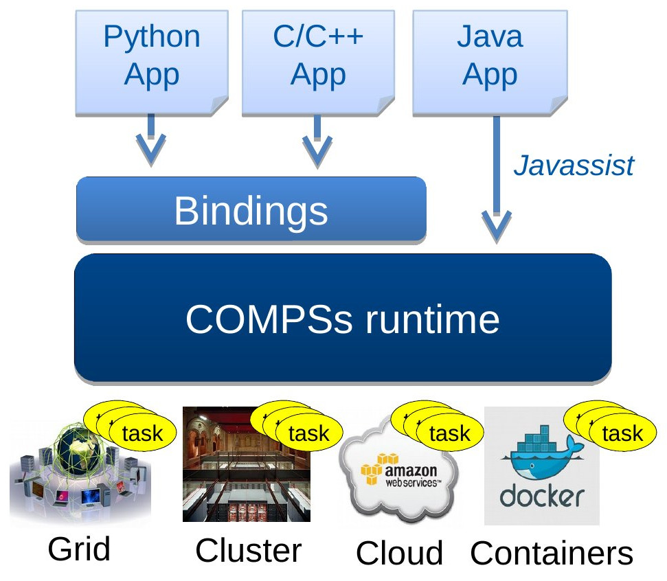
Additionally, the programming model is based on sequential programming which means that users do not need to deal with any parallelization and distribution issue such as thread creation, synchronization, data distribution, messaging or fault-tolerance. Instead, application developers only select which methods must be considered as tasks, and the runtime spawns them asynchronously on a set of resources instead of executing them locally and sequentially.

3.1.1 PyCOMPSs Programming Model

Regarding programmability, tasks are identified by inserting annotations in the form of Python decorators. These annotations are inserted at method level and indicate that invocations to a given method should become tasks at execution time. The @task decorator also contains information about the directionality of the method parameters specifying if a given parameter is read (IN), written (OUT) or both read and written in the method (INOUT).

Figure 2 shows an example of a task annotation. The parameter c has direction INOUT, and parameters a and b are set to the default direction IN. The directionality tags are used at execution time to derive the data dependencies between tasks and are applied at an object level, taking into account its references to identify when two tasks access the same object.

Additionally to the @task decorator, the @constraint decorator can be optionally defined to indicate some task hardware or software requirements. Continuing with the previous example, the task constraint ComputingUnits tells the runtime how many CPUs are consumed by each task execution. The available resources are defined by the system administrator in a separated XML configuration file. Other constraints that can be defined refer to the processor architecture, memory size, disk storage, operating system or available libraries.

⬇

@constraint(ComputingUnits=”$CUS”)

@task(c=INOUT)

def multiply(a, b, c):

c += a * b

Figure 2: Sample task annotation

A tiny synchronization API completes the PyCOMPSs syntax. As shown in Figure 3, the API function compss_wait_on waits for the completion of all the tasks modifying the result’s value and brings the final value to the node executing the main program. Then, the execution of the main program is resumed. Given that PyCOMPSs is used mostly in distributed environments, synchronization implies a data transfer from remote storage or memory space to the node executing the main program.

⬇

for block in data:

partial_res = wordcount_task(block)

reduce_task(result, partial_res)

final_result = compss_wait_on(result)

Figure 3: Sample call to synchronization API

3.2 PLUTO

Many compute-intensive scientific applications spend most of their execution time running nested loops. The Polyhedral Model [26] provides a powerful mathematical abstraction to analyze and transform loop nests in which the data access functions and loop bounds are affine combinations (linear combinations with a constant) of the enclosing loop iterators and parameters. As shown in Figure 4, this model represents the instances of the loop nests’ statements as integer points inside a polyhedron, where inter and intra-statement dependencies are characterized as a dependency polyhedron. Combining this representation with Linear Algebra and Integer Linear Programming, it is possible to reason about the correctness of a sequence of complex optimizing and parallelizing loop transformations.

Figure 4: Pluto overview. Source: Pluto’s official website [27]

PLUTO [27, 4] is an automatic parallelization tool based on the Polyhedral model to optimize arbitrarily nested loop sequences with affine dependencies. At compile time, it analyses C source code to optimize and parallelize affine loop-nests and automatically generate OpenMP C parallel code for multi-cores. Although the tool is fully automatic, many options are available to tune tile sizes, unroll factors, and outer loop fusion structure.

Figure 5: Pluto source-to-source transformation. Source:  [28]

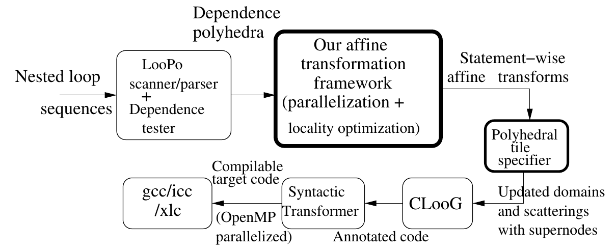
As shown in Figure 5, PLUTO internally translates the source code to an intermediate OpenScop [29] representation using CLAN [30]. Next, it relies on the Polyhedral Model to find affine transformations for coarse-grained parallelism, data locality, and efficient tiling. Finally, PLUTO generates the OpenMP C code from the OpenScop representation using CLooG [31]. We must highlight that the generated code is also optimized for data locality and made amenable to auto-vectorization.

3.2.1 Loop Tiling

Among many other options, PLUTO can tile code by specifying the --tile option. In general terms, as shown in Figure 6, tiling a loop of given size N results in a division of the loop in N/T repeatable parts of size T. For instance, this is suitable when fitting loops into the L1 or L2 caches or, in the context of this paper, when building the data blocks to increase the tasks’ granularity.

⬇

# Original loop # Tiled loop

for i in range(N): for i in range(N/T):

print(i) for t in range(T):

print(i*T + t)

Figure 6: Tiling example

Along with this option, users can let PLUTO set the tile sizes automatically using a rough heuristic, or manually define them in a tile.sizes file. This file must contain one tile size on each line and as many tile sizes as the loop nest depth.

In the context of parallel applications, tile sizes must be fine-tuned for each application so that they maximize locality while making sure there are enough tiles to keep all cores busy.

4 Architecture

The framework proposed in this paper eases the development of distributed applications by letting users program their application in a standard sequential fashion. It is developed on top of PyCOMPSs and PLUTO. When automatically parallelizing sequential applications, users must only insert an annotation on top of the potentially parallel functions to activate the AutoParallel module. Next, the application can be launched using PyCOMPSs.

Flag	Default Value	Description
pluto_extra_flags	None	List of flags for the internal PLUTO command
taskify_loop_level	0	Taskification loop depth (see Section 4.2)
force_autogen	True	When set to False, loads a previously generated code
generate_only	False	When set to True, only generates the parallel version of the code

TABLE I: List of flags for the @parallel() decorator

Following the same approach than PyCOMPSs, we have included a new decorator @parallel() to specify which methods should be automatically parallelized at runtime. Notice that functions using this decorator must contain affine loops so that the module can propose a parallelization. Otherwise, the source code will remain intact. Table I shows the valid flags for the decorator.

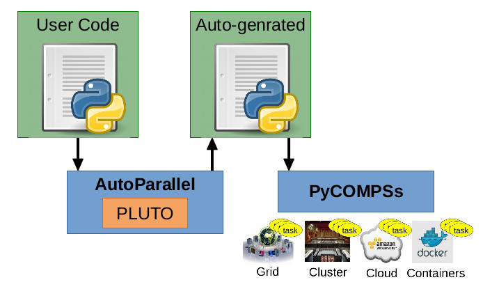
As shown in Figure 7, the AutoParallel Module analyzes the user code searching for @parallel() annotations. Essentially, when found, the module calls PLUTO to generate its parallelization and substitutes the user code by a newly generated code. Once all annotations have been processed, the new tasks are registered into PyCOMPSs, and the execution continues as a regular PyCOMPSs application (as described in Section 3.1). Finally, when the application has ended, the generated code is stored in a (_autogen.py) file and the user code is restored.

Figure 7: AutoParallel Module Overview

4.1 AutoParallel Module

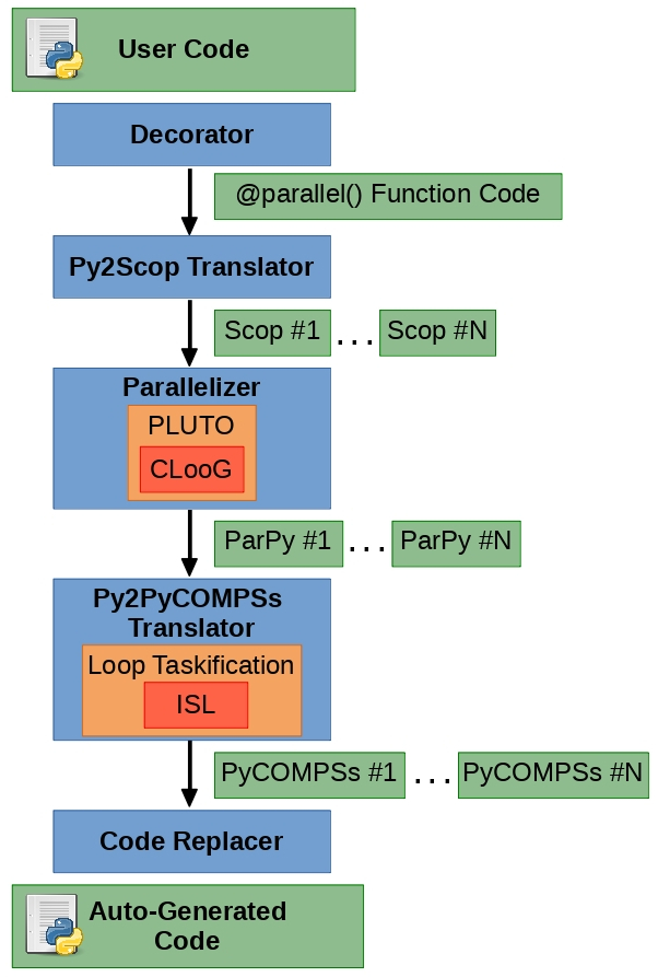
Next, we describe the five components of the AutoParallel module. For the sake of clarity, Figure 8 shows the relationship between all the components and its expected inputs and outputs.

Figure 8: AutoParallel Module Internals

• Decorator Implements the @parallel() decorator to detect functions that the user has marked as potentially parallel

• Python To OpenScop Translator For each affine loop nest detected in the user function, builds a Python Scop object representing it that can be bulked into an OpenScop format file.

• Parallelizer Returns the Python code resulting from parallelizing an OpenScop file. Since Python does not have any standard regarding parallel annotations, the parallel loops are annotated using comments with OpenMP syntax.

• Python to PyCOMPSs Translator Converts an annotated Python code into a PyCOMPSs application by inserting the necessary task annotations and data synchronizations. This component also performs loop taskification if it is enabled (see Section 4.2 for more details).

• Code Replacer Replaces each loop nest in the initial user code by the auto-generated code so that PyCOMPSs can execute the code in a distributed computing platform. When the application has finished, it restores the user code and saves the auto-generated code in a separated file.

For instance, Figure 9 shows the relevant parts of an Embarrassingly Parallel application with the main function annotated with the @parallel() decorator that contains two nested loops.

⬇

# Main Function

from pycompss.api.parallel import parallel

@parallel()

def ep(mat, n_size, m_size, c1, c2):

for i in range(n_size):

for j in range(m_size):

mat[i][j] = compute(mat[i][j], c1, c2)

# MAIN

if __name__ == ”__main__”:

# Parse arguments

…

# Initialize matrices

MAT = initialize_matrix(NSIZE, MSIZE)

# Begin computation

ep(MAT, NSIZE, MSIZE, COEF1, COEF2)

Figure 9: EP example: user code

⬇

# [COMPSs Autoparallel] Begin Autogenerated code

@task(var2=IN, c1=IN, c2=IN, returns=1)

def S1(var2, c1, c2):

return compute(var2, c1, c2)

def ep(mat, n_size, m_size, c1, c2):

if m_size >= 1 and n_size >= 1:

lbp = 0

ubp = m_size - 1

for t1 in range(lbp, ubp + 1):

lbv = 0

ubv = n_size - 1

for t2 in range(lbv, ubv + 1):

mat[t2][t1]=S1(mat[t2][t1],c1,c2)

compss_barrier()

# [COMPSs Autoparallel] End Autogenerated code

Figure 10: EP example: auto-generated code without loop taskification

In addition, Figure 10 shows its parallelization. Notice that the source code contains two nested loops with a single inner statement. It contains a task definition (with its data dependencies) that matches the original loop statement, a new main loop nest proposed by PLUTO (which exploits the inherent parallelism available in the original code), and a final barrier used as synchronization point.

4.2 Loop Taskification

Many compute-intensive scientific applications are not designed as block computations, and thus, the tasks proposed by the AutoParallel module are single statements. Although this can be harmless in tiny parallel environments, it leads to poor performances when executed using large distributed environments since the tasks’ granularity is not large enough to surpass the overhead of transferring the task definition, and the input and output data. To face this issue, we have extended the Python to PyCOMPSs Translator with support for loop taskification.

Essentially, loop taskification means processing the parallel code and converting into tasks all the loops of a certain depth of the loop nest. Since tasks may use N-dimensional arrays, this also implies to create the necessary data blocks (chunks) for each callee and revert them after the task execution. Continuing with the previous example, Figure 11 shows its parallelization with loop taskification.

⬇

# [COMPSs Autoparallel] Begin Autogenerated code

@task(lbv=IN, ubv=IN, c1=IN, c2=IN, returns=”LT2_args_size”)

def LT2(lbv, ubv, c1, c2, *args):

global LT2_args_size

var1, = ArgUtils.rebuild_args(args)

for t2 in range(0, ubv + 1 - lbv):

var1[t2] = S1_no_task(var1[t2], c1, c2)

return ArgUtils.flatten_args(var1)

def S1_no_task(var2, c1, c2):

return compute(var2, c1, c2)

def ep(mat, n_size, m_size, c1, c2):

if m_size >= 1 and n_size >= 1:

lbp = 0

ubp = m_size - 1

for t1 in range(lbp, ubp + 1):

lbv = 0

ubv = n_size - 1

# Chunk creation and flattening

LT2_aux_0 = [mat[t2][t1] for …]

LT2_au = ArgUtils()

global LT2_args_size

LT2_flat, LT2_args_size

= LT2_au.flatten(LT2_aux_0)

# Task call

LT2_ret = LT2(lbv, ubv, c1, c2,

*LT2_flat)

# Rebuild and re-assign

LT2_aux_0, = LT2_au.rebuild(LT2_ret)

…

compss_barrier()

# [COMPSs Autoparallel] End Autogenerated code

Figure 11: EP example: auto-generated code with loop taskification

Notice that the generated code with loop taskification is significantly more complex. The code defines a task containing the inner-most loop of the original code’ statements (only one in this case) and all its data dependencies accordingly. The main loop is also modified by chunking the necessary data for the task execution, flattening the data as a single dimension list, calling the task, rebuilding the chunks after the task callee, and re-assigning the values to the original variables. Notice that this last assignment is performed by pre-calculating the number of expected parameters and using PyCOMPSs Future Objects to avoid any synchronization in the master code (objects are only synchronized and transferred when required by a task execution). The end of the main code also includes a barrier as a synchronization point.

However, taskification may annihilate all the potential parallelism of the application (for instance, by setting taskify_loop_level=2 in the previous example). To prevent this, we have integrated PLUTO’s tiling transformation so that the loop taskification can be achieved on tiles.

4.3 Python Extension for CLooG

As described in Section 3.2, PLUTO operates internally with the OpenScop format. It relies on CLAN to translate input code from C/C++ or Fortran to OpenScop, and on CLooG to translate output code from OpenScop to C/C++ or Fortran.

Since we are targeting Python code, a translation from Python to OpenScop is required before calling PLUTO, and another translation from OpenScop to Python is required at the end. For the input, we have chosen to manually translate the code using the Python To OpenScop Translator component since CLAN is not adapted for supporting other language and PLUTO may take OpenScop format as input. We have extended CLooG so that the written output code is directly in Python: the language options were extended, and the Pretty Printer was modified in order to translate every OpenScop statement in its equivalent Python format. Since Python does not have any standard regarding parallel annotations, the parallel loops are annotated with comments in OpenMP syntax.

5 Experimentation

5.1 Computing Infrastructure

Results presented in this section have been obtained using the MareNostrum IV Supercomputer located at the Barcelona Supercomputing Center (BSC).

We have used PyCOMPSs version 2.3.rc1807 (available at [32]), PLUTO version 0.11.4, CLooG version 0.19.0, and AutoParallel version 0.2 (available at [33]). We have also used Intel®Python 2.7.13, Intel®MKL 2017, Java OpenJDK 8 131, GCC 7.2.0, and Boost 1.64.0.

All the benchmark codes used for this experimentation are also available at [34].

MareNostrum IV

The MareNostrum IV begun operating at the end of June 2017. Its current peak performance is 11.15 Petaflops, ten times more than its previous version, MareNostrum III. The supercomputer is composed by 3456 nodes, each of them with two Intel® Xeon Platinum 8160 (24 cores at 2,1 GHz each). It has 384.75 TB of main memory, 100Gb Intel®Omni-Path Full-Fat Tree Interconnection, and 14 PB of disk storage [35].

5.2 Blocked Applications

The first set of experiments has been designed to compare the application’s code automatically generated by the AutoParallel module (autoparallel version) against the one written by a PyCOMPSs expert user (userparallel version). To this end, we have used the LU, Cholesky, and QR decompositions described and analyzed in our previous work [16].

In general terms, the matrices are chunked in smaller square matrices (known as blocks) to distribute the data easily among the available resources so that the square blocks are the minimum entity to work with [36]. Furthermore, the initialization is performed in a distributed way, defining tasks to initialize the matrix blocks. These tasks do not take into account the nature of the algorithm, and they are scheduled in a round robin manner. Next, all the computations are performed considering that the data is already located on a given node.

Given a fixed matrix size, increasing the number of blocks increases the maximum parallelism of the application since blocks are the tasks’ minimum work entities. On the other hand, increasing the block size increases the tasks’ computational load which, at some point, will surpass the serialization and transfer overheads. Hence, the number of blocks and the block size for each application are a trade-off to fill all the available cores while maintaining acceptable performance.

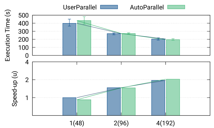
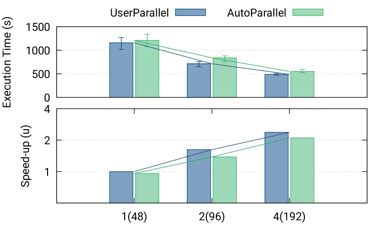
Next subsections analyze each application in depth, with a figure showing the execution results that contains two plots. For both plots, the horizontal axis shows the number of worker nodes (with 48 cores each) used for each execution, the blue color is the userparallel version and the green color is the autoparallel. The top plot represents the mean, maximum, and minimum execution times over 10 runs and the bottom plot represents the speed-up of each version with respect to the userparallel version running with a single worker.

5.2.1 Cholesky

The Cholesky factorization can be applied to Hermitian positive-defined matrices. This decomposition is a particular case of the LU factorization, obtaining two matrices of the form $U=L^{t}$. Our version of this application applies the right-looking algorithm [37] because it is more aggressive, meaning that in an early stage of the computation there are blocks of the solution that are already computed and all the potential parallelism is released as soon as possible.

Table II analyses the userparallel and autoparallel versions in terms of code complexity, loop configuration, and number of different task types. The code complexity is measured using the Babelfish Tools [38] and includes lines of code, cyclomatic complexity, and n-path. Although the generated code is not much larger than the original one, it is significantly more complex in terms of cyclomatic complexity and n-path. Notice that, although the autoparallel version has three 3-depth loop nests instead of a single loop nest with four loops, the maximum loop depth remains the same (three). Furthermore, regarding the amount of task calls, userparallel version includes three tasks (potrf, solve_triangular, and gemm), while the autoparallel version includes four tasks (that map to the previous operations plus an additional one to generate blocks initialized to zero).

Version	Code Analysis			Loops Analysis			Task Types
	LoC	CC	NPath	Main	Total	Depth
userparallel	220	26	112	1	4	3	3
autoparallel	274	36	14576	3	9	3	4

TABLE II: Cholesky code analysis

Figure 12 shows the execution results of the Cholesky decomposition over a dense matrix of $65536\times 65536$ elements decomposed in $32\times 32$ blocks with $2048\times 2048$ elements each. As explained at the beginning of this section, we have chosen 32 blocks because it is the minimum amount providing enough parallelism for 192 cores, and a bigger block size (e.g., $4096\times 4096$) was impossible due to memory constraints. The speed-up of both versions is limited by the block-size due to the small task granularity, reaching 2 when using 4 workers. Although the userparallel version spawns 6512 tasks and the autoparallel version spawns 7008 tasks, the execution times and the overall performance of both versions are almost the same. This is due to the fact that the autoparallel version spawns an extra task per iteration to initialize blocks to zero on the matrix’s lower triangle that has no impact in the overall computation time.

Figure 12: Cholesky decomposition: Execution times and speed-up

5.2.2 LU

For the LU decomposition, an approach without pivoting [39] has been the starting point. However, since this approach might be unstable in general [40], some modifications have been included to increase the stability of the algorithm while keeping the block division and avoiding bringing an entire column into a single node.

As shown in Table III, both versions have two main loops with a maximum depth of three and a total of six nested loops. However, the autoparallel version has 315% more paths in the flow than the userparallel because it has different optimization codes for different variable values. Regarding the task types, the userparallel version contains calls to four different tasks: multiply, invert_triangular, dgemm, and custom_lu. On the other hand, the autoparallel version generates twelve different task types because it generates one task type per statement in the original loop, even if the statement contains the same task call. For instance, the original LU contains four calls to the invert_triangular function that are detected as different statements and converted to different task types.

Version	Code Analysis			Loops Analysis			Task Types
	LoC	CC	NPath	Main	Total	Depth
userparallel	238	35	79872	2	6	3	4
autoparallel	320	39	331776	2	6	3	12

TABLE III: LU code analysis

Figure 13 shows the execution results of the LU decomposition with a $49152\times 49152$ dense matrix of $24\times 24$ blocks with $2048\times 2048$ elements each. As in the previous example, the overall performance is limited by the block size. This time the userparallel version slightly outperforms the autoparallel version; achieving, respectively, a 2.45 and 2.13 speed-up with 4 workers (192 cores).

Figure 13: LU decomposition: Execution times and speed-up

Figure 14: LU decomposition: Paraver trace. At left, userparallel and, at right, the autoparallel version

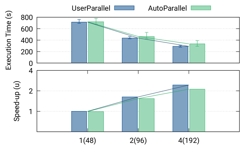
Regarding the number of tasks, the userparallel version spawns 14676 tasks while the autoparallel version spawns 15227 tasks. This difference is due to the fact that the autoparallel version initializes distributedly an intermediate zero matrix, while the userparallel initializes it in the master memory.

Figure 14 shows a detailed Paraver trace of both versions running with 4 workers (192 cores). The autoparallel version (right) is more coloured because it has more tasks although, as previously explained, they execute the same function in the end. Notice that the performance degradation of the autoparallel version is due to the fact that the maximum parallelism is lost before the end of the execution. On the contrary, the userparallel version maintains the maximum parallelism until the end of the execution.

5.2.3 QR

Unlike traditional QR algorithms that use the Householder transformation, our implementation uses a method based on Givens rotations [41]. This way, data can be accessed by blocks instead of columns.

The QR decomposition represents one of the most complex use cases in terms of data dependencies thus, having a high cyclomatic complexity. As shown in Table IV, the generated code differs significantly in terms of loop configurations but not regarding code since the autoparallel version has similar cyclomatic complexity, 34% more lines of code, and 51% more paths. Although the maximum loop depth remains the same, the auto-generated code has two main loops instead of one. Regarding the task types, while the userparallel version has four tasks (namely qr, dot, little_qr, and multiply_single_block), the autoparallel version has twenty different task types.

Version	Code Analysis			Loops Analysis			Task Types
	LoC	CC	NPath	Main	Total	Depth
userparallel	303	41	168	1	6	3	4
autoparallel	406	43	344	2	7	3	20

TABLE IV: QR code comparison

Figure 15 shows the execution results of the QR decomposition with a $32768\times 32768$ matrix of $16\times 16$ blocks with $2048\times 2048$ elements each. The autoparallel version spawns 26304 tasks and the userparallel version spawns 19984 tasks. As in the previous examples, the overall performance is limited by the block size. However, the userparallel version slightly outperforms the autoparallel version; achieving a 2.37 speed-up with 4 workers instead of 2.10. The difference is mainly because the autoparallel version spawns four copy tasks per iteration (copy_reference), while the userparallel version executes this code in the master side copying only the reference of a future object.

Figure 15: QR decomposition: Execution times and speed-up

5.3 Fine-grain Applications

The second set of experiments is designed to evaluate the capability of generating distributed code from a purely sequential code. To this end, we have implemented a Python version of many applications from the Polyhedral Benchmark suite [42].

As discussed in next subsections, this approach provides several advantages in terms of code re-organization and data blocking but, in its current state, has still significant performance issues. Hence, this paper only presents a preliminary evaluation of the GEMM application.

5.3.1 GEMM

The presented implementation of the General Matrix-Matrix product of general rectangular matrices with float complex elements performs: $C=\alpha\cdot A\cdot B+\beta\cdot C$. In general terms, the arrays and matrices are implemented as plain NumPy arrays or matrices. This means that there are no blocks and thus, the minimum work entity is a single element (a float). As in the previous set of experiments, the initialization is performed in a distributed way (defining tasks to initialize the matrix elements), and the computations are performed considering that the data is already located in a given node.

We have evaluated a userparallel Fine-Grain version and an autoparallel version built using loop taskification. For comparison purposes, we have also evaluated a userparallel Blocked version. Although the userparallel FG works with single elements and userparallel B with blocks, both versions include 2 tasks: scale, and multiply. The autoparallel LT version defines four tasks: the two original ones and their two loop-tasked versions. The original tasks are kept because, in configurations that do not use PLUTO’s tiles, it is possible to find function calls that cannot be loop-taskified. However, in this case, only the loop-tasked versions are called during the execution. Concerning the code, as shown in Table V, the Loop Tasking version is significantly more complex in terms of lines of code, cyclomatic complexity, and n-path, but is capable of splitting the main loop into two loops (one for the scaling operations and another for the multiplications) for better parallelism.

Version	Code Analysis			Loops Analysis			Task Types
	LoC	CC	NPath	Main	Total	Depth
UserP. FG	194	22	112	1	4	3	2
UserP. B	189	22	112	2	5	3	2
AutoP. LT	382	133	360064	2	4	3	4

TABLE V: Gemm code comparison

Figure 16 shows the execution results of the GEMM application with a matrix of $64\times 64$ elements with 1 worker (48 cores). For the autoparallel, the tile sizes are set to 8 and, for the blocked userparallel, the matrix has $8\times 8$ blocks with $8$ elements each. The left plot shows the execution time of the userparallel FG (blue) and the autoparallel LT (green). The right plot shows the slow-down of both versions with respect to the blocked userparallel B version running with a single worker.

Figure 16: GEMM: Execution times and slow-down

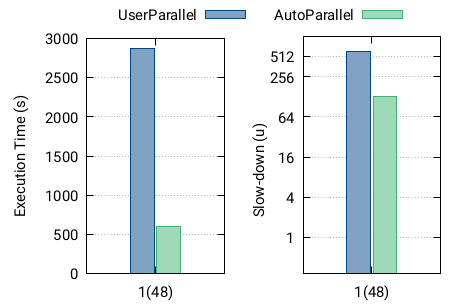
Although both performances are completely unacceptable, there is still room for comparison. First, the autoparallel version is capable of splitting the main loop to isolate the scaling operations. Second, defining single elements as the minimum task entity leads to tasks with too little computation that cause a massive overhead of serialization and transfer inside PyCOMPSs. On the other hand, automatically building data blocks from the sequential user code improves almost 5 times the application performance. More in-depth, building data blocks helps PyCOMPSs to surpass the serialization and transfer overheads. However, building data blocks also increases significantly the number of parameters of each task (around $8\times 8\times 3=192$ parameters per task) which slows down the PyCOMPSs scheduler and task manager.

We believe that Loop Tasking is a good approach for this kind of applications provided that PyCOMPSs is enhanced with support for collections. This means that task parameters should be defined as lists of objects that are handled by the PyCOMPSs runtime as a single entity. This would significantly lower the scheduling, serialization, and transferring overheads.

6 Conclusions and Future Work

This paper has presented and evaluated AutoParallel, a Python module to automatically parallelize affine loop nests and execute them on distributed infrastructures. Built on top of PyCOMPSs and PLUTO, it is based on sequential programming so that anyone can scale up an application to hundreds of cores. Instead of manually taskifying a sequential python code, the users only need to add a @parallel annotation to the methods containing affine loop nests.

The evaluation shows that the codes automatically generated by the AutoParallel module for the Cholesky, LU, and QR applications can achieve the same performance than the manually parallelized versions. Thus, AutoParallel goes one step further in easing the development of distributed applications.

As future work, although the Loop Taskification provides an automatic way to create blocks from sequential applications, its performance is still far from acceptable. On the one hand, we will do research on how to simplify the chunk accesses from the AutoParallel module. On the other hand, we will extend PyCOMPSs to support collection objects (e.g., lists) with different sizes so that we could avoid flattening and rebuilding of chunks, and serializing each object in a separate file.

Finally, AutoParallel could be integrated with different tools similar to PLUTO to support a larger scope of loop nests. For instance, APOLLO [43, 44] provides automatic, dynamic and speculative parallelization and optimization of programs’ loop nests of any kind (for, while or do-while loops). However, its integration would require PyCOMPSs to be extended with some speculative mechanisms.

Appendix A Artifact Description

A.1 Abstract

This description contains the information required to launch the experiments of the SC18 paper ”AutoParallel: A Python module for automatic parallelization and distributed execution of affine loop nests”. More precisely, we explain how to install the AutoParallel module and its dependencies, and how to run the experiments described in Section 5.

A.2 Description

A.2.1 Check-list (artifact meta information)

• Program: Python application, Python binding, Java Runtime, C and C++ libraries

• Run-time environment: AutoParallel 0.2, PyCOMPSs 2.3.rc1807, PLUTO 0.11.4, Python 2.7.13, Java OpenJDK 8 131, GCC 7.2.0, Boost 1.64.0

• Output: Time to solution and number of tasks

• Experiment workflow: Prepare system, clone PyCOMPSs, load submodules, install PyCOMPSs, install PLUTO, install the AutoParallel module, run the examples, and observe the results

• Experiment customization: Input dataset size, number of nodes, number of cores, maximum node memory, PLUTO tile sizes, and PyCOMPSs scheduler, log level, communication adaptor, and workers working directory

• Publicly available?: Yes

A.2.2 How delivered

PyCOMPSs and the AutoParallel module can be cloned from GitHub using [32] and [33] respectively. The examples used for the experimentation can be found under the examples folder.

A.2.3 Hardware dependencies

None.

A.2.4 Software dependencies

PyCOMPSs depends on the COMPSs Runtime, the Python and Commons bindings, and the Extrae tracing module that are automatically installed. However, the users must provide valid Java, Python, and GCC installations.

PLUTO depends on Candl, Clan, CLooG, ISL, OpenScop, PipLib, and PolyLib modules that are automatically installed. However, the users must explicitly provide valid GMP, Flex, and Bison installations.

The AutoParallel module requires a valid installation of PyCOMPSs and PLUTO. Moreover, the users must check that the following Python modules are available: AST, ASTOR, enum34, logging, inspect, islPy, symPy, subprocess, and unittest.

The examples used for the experimentation require the NumPy Python module.

A.2.5 Datasets

The datasets of each application are pseudo-randomly generated during the execution since the size is the only relevant parameter for the computational results. However, the users can check the correctness of the algorithms against the their sequential version by using the -d option when invoking the run scripts.

A.3 Installation

1. Prepare the system

   ⬇

   # Runtime dependencies

   $ sudo apt-get install openjdk-8-jdk uuid-runtime curl wget openssh-server maven graphviz xdg-utils

   $ export JAVA_HOME=<path_to_openjdk>

   # Python and Commons bindings dependencies

   $ sudo apt-get install libtool automake build-essential python-dev libpython2.7 python-pip libboost-all-dev libxml2-dev csh

   $ sudo pip2 install numpy dill decorator

   # Extrae tracing module dependencies

   $ sudo apt-get install libxml2 gfortran libpapi-dev papi-tools

   # AutoParallel and PLUTO dependencies

   $ sudo apt-get install libgmp3-dev flex bison libbison-dev texinfo

   $ sudo pip2 install astor enum34 islpy sympy

2. Clone PyCOMPSs and enter the newly created directory

   ⬇

   $ git clone https://github.com/bsc-wdc/compss.git

   $ cd compss

3. Initialize and patch the submodules (PLUTO, AutoParallel, and Extrae)

   ⬇

   $ ./submodules_get.sh

   $ ./submodules_patch.sh

4. Install everything (a) into a given target location or (b) into the default location /opt/COMPSs (requires root privileges)

   ⬇

   $ cd builders

   $ (a) ./buildlocal $HOME/COMPSs

   $ (b) sudo -E ./buildlocal

5. Check up the environment

   ⬇

   $ runcompss -v

   COMPSs version 2.3 Daisy

A.4 Experiment workflow

Once that PyCOMPSs, PLUTO, and the AutoParallel module are installed, any example can be executed. To ensure that everything runs smoothly, the users should use the prepared scripts: the run.sh for laptops and the enqueue.sh, and experiments.sh scripts for supercomputers.

More in detail, each application contains:

• README.md : File describing the application and its commands

• autoparallel : Folder containing the autoparallel version of the application

  • app_name.py : Source file of the autoparallel version of the application

  • app_name_autogen.py : Source file automatically generated

  • run.sh : Script to run the autoparallel version of the application

• userparallel : Folder containing the userparallel version of the application

  • app_name.py : Source file of the userparallel version of the application

  • run.sh : Script to run the userparallel version of the application

• run.sh : Script to run the all the versions of the application

• enqueue.sh : Script to enqueue the application to a queue system (SLURM, LSF, or PBS)

• experiments.sh : Script to run all the experiments with all the versions of the application

• results.sh : Script to parse the experiments results

In the rest of the artifact description, we will explain the most important options to set up in order to reproduce the results of the paper.

A.5 Evaluation and expected result

On the one hand, the run.sh script is prepared to run executions on laptops. Although it can be simply invoked without parameters (setting up the default values), the script is a wrapper of the runcompss command and accepts many additional flags (e.g., -d for debug). For instance, here is the command to execute the Cholesky application:

⬇

$ cd examples/cholesky

$ ./run.sh

Two executions will be triggered; one for the autoparallel and another for the userparallel version. The output for the Cholesky example should include the following lines:

⬇

RESULTS —————–

VERSION AUTOPARALLEL

MSIZE 4

BSIZE 4

DEBUG False

TOTAL_TIME 3.91822195053

INIT_TIME 3.22278118134

CHOLESKY_TIME 0.695440769196

————————-

⬇

[(5330) API] - – COMPSs Task Execution Summary –

…

[(5331) API] - Total executed tasks: 36

[(5331) API] - ———————————–

The results section provides information about the application execution, such as the application parameters and the computation time (CHOKESKY_TIME in the example). The execution summary shows, between others, the total number of executed tasks. Furthermore, inside the results folder the users will find the paraver traces and the task dependency graphs:

⬇

$ cd examples/cholesky/results/local/

$ okular autoparallel/complete_graph.pdf

$ okular userparallel/complete_graph.pdf

$ wxparaver autoparallel/trace/*.prv

$ wxparaver userparallel/trace/*.prv

On the other hand, the enqueue.sh, and experiments.sh scripts are prepared to run executions on supercomputers. The first is a wrapper of the enqueue_compss to enqueue a single execution of the application. The users must specify version (autoparallel or userparallel), job dependency, number of nodes, wall-clock time, number of cpus per node, tracing value, graph value, log level, and the application parameters (in the Cholesky example: the matrix size and block size).

⬇

$ ./enqueue.sh autoparallel None 2 150 48 true false off 32 2048

The experiments.sh script enqueues several jobs to reproduce the experimentation described in Section 5 and can be run without arguments. The results can be easily summarized to a CSV file by running the results.sh script, that will create a results folder with a results.summary file inside containing:

⬇

JOB_ID VERSION MSIZE BSIZE TRACING NUM_WORKERS TOTAL_TIME INIT_TIME COMP_TIME NUM_TASKS

2210018 autoparallel 32 2048 true 1 520,067487001 93,8065400124 426,260946989 7008

A.6 Experiments Customization

The application parameters can be modified inside the corresponding experiments.sh script of each application. Moreover, the PyCOMPSs options can be tuned inside the corresponding enqueue.sh script.

References

- [1] S. Cass, “The 2017 Top Programming Languages (IEEE Spectrum),” https://spectrum.ieee.org/computing/software/the-2017-top-programming-languages, 2017, accessed: 2018-02-14.
- [2] G. Van Rossum and F. L. Drake, Python language reference manual. Network Theory, 2003.
- [3] “The Go Programming Language,” Website at https://golang.org/, (Date of last access: 4th June, 2018).
- [4] U. Bondhugula, A. Hartono, J. Ramanujam, and P. Sadayappan, Automatic Transformations for Communication-Minimized Parallelization and Locality Optimization in the Polyhedral Model. Springer Berlin Heidelberg, 4 2008, pp. 132–146. [Online]. Available: https://doi.org/10.1007/978-3-540-78791-4_9
- [5] S. v. d. Walt, S. C. Colbert, and G. Varoquaux, “The NumPy Array: A Structure for Efficient Numerical Computation,” Computing in Science and Engg., vol. 13, no. 2, pp. 22–30, 3 2011. [Online]. Available: https://doi.org/10.1109/MCSE.2011.37
- [6] E. Jones, T. Oliphant, and P. Peterson, “SciPy: Open source scientific tools for Python,” 2001–. [Online]. Available: http://www.scipy.org/
- [7] “BLAS (Basic Linear Algebra Subprograms),” Website at http://www.netlib.org/blas/, (Date of last access: 28th August, 2017).
- [8] E. Anderson, Z. Bai, C. Bischof, L. S. Blackford, J. Demmel, J. Dongarra, J. Du Croz, A. Greenbaum, S. Hammarling, A. McKenney et al., LAPACK Users’ guide. SIAM, 1999.
- [9] L. Dagum and R. Menon, “OpenMP: An Industry-Standard API for Shared-Memory Programming,” IEEE Comput. Sci. Eng., vol. 5, no. 1, pp. 46–55, 1 1998. [Online]. Available: https://doi.org/10.1109/99.660313
- [10] “Threading Building Blocks (Intel®TBB),” Website at https://www.threadingbuildingblocks.org/, (Date of last access: 28th August, 2017).
- [11] “Parallel Processing and Multiprocessing in Python,” Website at https://wiki.python.org/moin/ParallelProcessing, (Date of last access: 10th October, 2017).
- [12] “Parallel Python Software,” Website at http://www.parallelpython.com, (Date of last access: 10th October, 2017).
- [13] L. Dalcín, R. Paz, and M. Storti, “MPI for Python,” Journal of Parallel and Distributed Computing, 2005. [Online]. Available: http://www.sciencedirect.com/science/article/pii/S0743731505000560
- [14] Dask Development Team, Dask: Library for dynamic task scheduling, 2016. [Online]. Available: http://dask.pydata.org
- [15] “PySpark,” Website at https://spark.apache.org/docs/latest/api/python/index.html, (Date of last access: 6th October, 2017).
- [16] R. Amela, C. Ramon-Cortes, J. Ejarque, J. Conejero, and R. M. Badia, “Enabling Python to Execute Efficiently in Heterogeneous Distributed Infrastructures with PyCOMPSs,” in Proceedings of the 7th Workshop on Python for High-Performance and Scientific Computing. New York, NY, USA: ACM, 2017, pp. 1:1–1:10. [Online]. Available: https://doi.org/10.1145/3149869.3149870
- [17] ——, “Executing linear algebra kernels in heterogeneous distributed infrastructures with PyCOMPSs,” Oil —& Gas Science and Technology - Revue d’IFP Energies Nouvelles (OGST), 2018.
- [18] W. McKinney, “Pandas: a Foundational Python Library for Data Analysis and Statistics,” Python for High Performance and Scientific Computing, pp. 1–9, 2011.
- [19] M. Zaharia, M. Chowdhury, M. J. Franklin, S. Shenker, and I. Stoica, “Spark: Cluster Computing with Working Sets,” in Proceedings of the 2Nd USENIX Conference on Hot Topics in Cloud Computing, Berkeley, CA, USA, 2010.
- [20] R. M. Badia and et al., “COMP superscalar, an interoperable programming framework,” SoftwareX, vol. 3, pp. 32–36, 12 2015. [Online]. Available: https://doi.org/10.1016/j.softx.2015.10.004
- [21] F. Lordan, R. M. Badia, and et al., “ServiceSs: an interoperable programming framework for the Cloud,” Journal of Grid Computing, vol. 12, no. 1, pp. 67–91, 3 2014. [Online]. Available: https://digital.csic.es/handle/10261/132141
- [22] S. Liang, Java Native Interface: Programmer’s Guide and Reference, 1st ed. Boston, MA, USA: Addison-Wesley Longman Publishing Co., Inc., 1999.
- [23] C. Ramon-Cortes, A. Serven, J. Ejarque, D. Lezzi, and R. M. Badia, “Transparent Orchestration of Task-based Parallel Applications in Containers Platforms,” Journal of Grid Computing, vol. 16, no. 1, pp. 137–160, 2018.
- [24] “Extrae Tool (Barcelona Supercomputing Center),” Website at https://tools.bsc.es/extrae, (Date of last access: 20th July, 2017).
- [25] “Paraver Tool (Barcelona Supercomputing Center),” Website at https://tools.bsc.es/paraver, (Date of last access: 20th July, 2017).
- [26] A. Cohen and et al., “Facilitating the Search for Compositions of Program Transformations,” in Proceedings of the 19th Annual International Conference on Supercomputing. ACM, 2005, pp. 151–160. [Online]. Available: https://doi.org/10.1145/1088149.1088169
- [27] “Pluto,” Website at http://pluto-compiler.sourceforge.net/, (Date of last access: 28th November, 2017).
- [28] U. Bondhugula, A. Hartono, J. Ramanujam, and P. Sadayappan, “A Practical Automatic Polyhedral Parallelizer and Locality Optimizer,” SIGPLAN Not., vol. 43, no. 6, pp. 101–113, 6 2008. [Online]. Available: http://doi.org/10.1145/1379022.1375595
- [29] C. Bastoul, “OpenScop: A Specification and a Library for Data Exchange in Polyhedral Compilation Tools,” Paris-Sud University, France, Tech. Rep., 9 2011. [Online]. Available: http://icps.u-strasbg.fr/people/bastoul/public_html/development/openscop/docs/openscop.html
- [30] C. Bastoul, A. Cohen, S. Girbal, S. Sharma, and O. Temam, Putting Polyhedral Loop Transformations to Work. Springer Berlin Heidelberg, 2004, pp. 209–225. [Online]. Available: https://doi.org/10.1007/978-3-540-24644-2_14
- [31] C. Bastoul, “Code Generation in the Polyhedral Model Is Easier Than You Think,” in PACT’13 IEEE International Conference on Parallel Architecture and Compilation Techniques. IEEE Computer Society, 9 2004, pp. 7–16. [Online]. Available: https://doi.org/10.1109/PACT.2004.11
- [32] “COMPSs GitHub,” Website at https://github.com/bsc-wdc/compss, (Date of last access: 4th June, 2018).
- [33] “PyCOMPSs AutoParallel Module GitHub,” Website at https://github.com/cristianrcv/pycompss-autoparallel, (Date of last access: 4th June, 2018).
- [34] “Experimentation GitHub,” Website at https://github.com/cristianrcv/pycompss-autoparallel/tree/master/examples, (Date of last access: 4th June, 2018).
- [35] “MareNostrum IV Technical Information,” Website at https://www.bsc.es/marenostrum/marenostrum/technical-information, (Date of last access: 4th June, 2018).
- [36] J. A. Gunnels, F. G. Gustavson, G. M. Henry, and R. A. van de Geijn, “FLAME: Formal Linear Algebra Methods Environment,” ACM Trans. Math. Softw., vol. 27, no. 4, pp. 422–455, 12 2001. [Online]. Available: https://doi.org/10.1145/504210.504213
- [37] P. Bientinesi, B. Gunter, and R. A. v. d. Geijn, “Families of Algorithms Related to the Inversion of a Symmetric Positive Definite Matrix,” ACM Trans. Math. Softw., vol. 35, no. 1, pp. 3:1–3:22, 7 2008. [Online]. Available: https://doi.org/10.1145/1377603.1377606
- [38] “Babelfish Tools,” Website at https://github.com/bblfsh/tools, (Date of last access: 23th August, 2018).
- [39] G. H. Golub and C. F. Van Loan, Matrix Computations (3rd Ed.). Baltimore, MD, USA: Johns Hopkins University Press, 1996.
- [40] J. W. Demmel and N. J. Higham, “Stability of Block Algorithms with Fast Level-3 BLAS,” ACM Trans. Math. Softw., vol. 18, no. 3, pp. 274–291, 9 1992. [Online]. Available: http://doi.org/10.1145/131766.131769
- [41] G. Quintana-Orti, E. S. Quintana-Orti, E. Chan, R. A. van de Geijn, and F. G. Van Zee, “Scheduling of QR Factorization Algorithms on SMP and Multi-Core Architectures,” in Proceedings of the 16th Euromicro Conference on Parallel, Distributed and Network-Based Processing (PDP 2008), ser. PDP ’08. IEEE Computer Society, 2008, pp. 301–310. [Online]. Available: https://doi.org/10.1109/PDP.2008.37
- [42] “PolyBench/C: The Polyhedral Benchmark suite,” Website at http://web.cse.ohio-state.edu/~pouchet.2/software/polybench/, (Date of last access: 18th June, 2018).
- [43] A. Sukumaran-Rajam and P. Clauss, “The Polyhedral Model of Nonlinear Loops,” ACM Trans. Archit. Code Optim., vol. 12, no. 4, pp. 48:1–48:27, Dec. 2015. [Online]. Available: http://doi.acm.org/10.1145/2838734
- [44] J. M. Martinez Caamaño, M. Selva, P. Clauss, A. Baloian, and W. Wolff, “Full runtime polyhedral optimizing loop transformations with the generation, instantiation, and scheduling of code-bones,” Concurrency and Computation: Practice and Experience, vol. 29, no. 15, p. e4192, 2017. [Online]. Available: https://onlinelibrary.wiley.com/doi/abs/10.1002/cpe.4192