A rare event algorithm links transitions in turbulent flows with activated nucleations

Abstract

Many turbulent flows undergo drastic and abrupt configuration changes with huge impacts. As a paradigmatic example we study the multistability of jet dynamics in a barotropic beta plane model of atmosphere dynamics. It is considered as the Ising model for Jupiter troposphere dynamics. Using the adaptive multilevel splitting, a rare event algorithm, we are able to get a very large statistics of transition paths, the extremely rare transitions from one state of the system to another. This new approach opens the way for addressing a set of questions that are out of reach through direct numerical simulations. We demonstrate for the first time the concentration of transition paths close to instantons, in a numerical simulation of genuine turbulent flows. We show that the transition is a noise-activated nucleation of vorticity bands. We address for the first time the existence of Arrhenius laws in turbulent flows. The methodology we developed shall prove useful to study many other transitions related to drastic changes for the turbulent dynamics of climate, geophysical, astrophysical and engineering applications. This opens a new range of studies impossible so far, and bring turbulent phenomena in the realm of non-equilibrium statistical mechanics.

Many turbulent flows undergo drastic and abrupt configuration changes with huge impacts Sommeria (1986); Ravelet et al. (2004); Berhanu et al. (2007); Wei et al. (2015); Zimmerman et al. (2011); Huisman et al. (2014); Pomeau (2016). The Earth magnetic field reverses on geological time scales due to turbulent motion of the Earth’s metal core Berhanu et al. (2007), wall flows transition from laminar to turbulent Pomeau (2016); Barkley et al. (2015); Shih et al. (2015), experiments in convection turbulence show bistability Wei et al. (2015); Zimmerman et al. (2011); Huisman et al. (2014), global climate changes like the glacial-interglacial transitions or the Dansgaard–Oeschger events are related to the turbulent oceans and atmosphere coupled to ice and carbon dioxide dynamics Rahmstorf et al. (2002). Is the kinetics and phenomenology of these turbulent transitions analogous to phase transitions in condensed matter, and rare conformational changes of molecules in chemistry and biochemistry? These key questions have not been addressed so far because of the difficulty related to the numerical complexity: We need both a proper turbulence representation and run extremely long simulations to observe transitions. In this letter we show that a new numerical approach based on rare event algorithms improves exponentially our capabilities. With this tool, we make the first numerical study of metastability and spontaneous transitions for a genuine turbulent dynamics. We study atmospheric turbulent jet transitions, relevant to describe abrupt climate changes on Jupiter’s troposphere.

Jupiter pictures show fascinating zonal bands whose color are correlated with the troposphere flow vorticity. Those bands correspond to East-West (zonal) velocity jets, which are stationary for centuries. During the period 1939-1940 a fantastic phenomenon occurred: the planet lost one of its jets Rogers (1995), which was replaced by three white anticyclones. Phil Marcus subsequently called this event a Jupiter’s sudden climate change Marcus (2004). This rare event is one example among thousands of sudden transitions betwee attractors in the self-organization of billions of vortices in turbulent flows. In this letter, we study the barotropic beta-plane quasi-geostrophic equations: the simplest model that describes the turbulent atmosphere jet self-organization Vallis and Maltrud (1992); Dritschel and McIntyre (2008); Galperin et al. (2001); Farrell and Ioannou (2007); Tobias and Marston (2013); Srinivasan and Young (2011). It is the Ising model of atmosphere dynamics: the simplest model to describe jet formation, although too simple to be quantitatively realistic.

The dimensionless version of the model equations read

$$\partial_{t}\omega+\mathbf{v}\cdot\mathbf{\nabla}\omega+\beta v_{y}=-\alpha\omega-\nu_{n}\left(-\Delta\right)^{n}\omega+\sqrt{2\alpha}\eta,$$ (1)

where $\mathbf{v}=\mathbf{e}_{z}\times\mathbf{\nabla}\psi$ is the non-divergent velocity, $v_{y}$ the North-South velocity component, $\omega=\Delta\psi$ and $\psi$ are the vorticity and the streamfunction, respectively, $\alpha$ is a linear friction coefficient, see Supplemental Material for the dimensional equations. The noise $\eta$ forces the flow dynamics and is precisely defined in the Supplemental Material file. When $\beta=0$, those equations are the two-dimensional stochastic Navier–Stokes equations for which a few rare transitions have been observed in the past between dipole and jet states Bouchet and Simonnet (2009), and for which impressive explicit relation between the energy injection rate and the Reynolds stresses have been recently derived Laurie et al. (2014); Kolokolov and Lebedev (2016a, b). Such relations have been further justified and extended to the case $\beta\neq 0$ Woillez and Bouchet (2017), see also Srinivasan and Young (2011). For $\beta\neq 0$ and for small enough $\alpha$ the vorticity dynamics self-organizes into zonal bands like on Jupiter (Fig. 1). The dimensionless parameter $\beta$ is proportional to $\beta_{d}$ that measures the local variations of the Coriolis parameter, and is related to the Rhines scale, defined in the Supplementary Materials. The number of jets roughly scales like $\beta^{1/2}$ Dritschel and McIntyre (2008). Fig. 1 shows metastable turbulent states with either two or three alternating jets, for two different values of $\beta$.

Figure 1: Right panels: typical snapshots of the vorticity fields (the colors show the vorticity values, with red for positive ones, blue for negative ones and black for intermediate ones; the range of vorticity is [-1,1]). Middle panels: Hovmöller diagrams of zonally averaged vorticity (the horizontal axis is $\alpha t$, the vertical one is $y$, and the color represents the $x-$averaged vorticity, $\alpha=1.20\ 10^{-3}$). Left panels: time and zonally averaged vorticity (red) and velocity (green). The top plots show a two jet state for $\beta=5$, while the bottom ones show a three jet one for $\beta=10$.

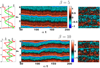
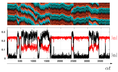
When $\beta$ is increased, one expects to see transitions from attractors with $2$ to $3$ alternating jets ($2\rightarrow 3$ transitions). As there is no related symmetry breaking, one may expect these transitions to be first order ones with discontinuous jumps of some order parameters. In situations with discontinuous transitions when an external parameter $\beta$ is changed, one expects for each bifurcation a multistability range $(\beta_{1},\beta_{2})$ in which two (or more) possible states exist for a single value of $\beta$. Such a bistability has indeed been observed Farrell and Ioannou (2007), by changing the model initial conditions. Fig. 2 shows for the first time spontaneous transitions between the two bistable states. The transitions are well characterized by the Fourier components $q_{n}=\int\mbox{d}x\mbox{d}y\,\omega(x,y)\mbox{e}^{iny}/(2\pi)^{2}$ for $n=2$ and $n=3$: Fig. 2 features five $2\to 3$ transitions, and five $3\to 2$ transitions in about $10^{6}$ turnover times.

Figure 2: Rare transitions between turbulent attractors with respectively 2 and 3 alternating jets. Upper panel: Hovmöller diagram of the zonal mean vorticity. Lower panel: timeseries of the modulus of $q_{2}$ (red) and $q_{3}$ (black), the zonal mean vorticity Fourier components, for wavenumber 2 and 3 respectively, versus the rescaled time $\alpha t$ ($\alpha=1.2\cdot 10^{-3}$ and $\beta=5.26$).

We would like to address the following basic questions: What are the transition rates? What are the relative probability of each attractors (equilibrium constants)? Do the transition trajectories concentrate close to instantons like in statistical physics Bouchet et al. (2016)? Do the thousands of small scale vortices act collectively as atoms in a nucleation process? Unfortunately, such questions are unaffordable using direct numerical simulations. Observing such rare spontaneous transitions in turbulent flows is highly unusual as most turbulent simulations last a few turnover times at most, because of the huge numerical cost. This limitation is a wall that drastically limits the study of transitions in turbulent flows to extremely simple models and a few transitions only. In order to study rare transitions in turbulent flows, we consider a completely new approach in turbulence studies: using the adaptive multilevel splitting algorithm Cérou and Guyader (2007); Bréhier et al. (2015); Rolland et al. (2016) (see Fig. 3). This rare event algorithm belongs to the family of splitting algorithms, where an ensemble of trajectories are simulated and subjected to a succession of selections, cloning or killing, and dynamical mutation steps. The principle of the algorithm Cérou and Guyader (2007) is described in the legend of Fig. 3. A full description of the algorithm and of the method to compute transition rates is described in Rolland et al. (2016). Its mathematical properties (convergence, fluctuations, etc) have been studied recently Bréhier et al. (2015); Cérou and Guyader (2016). This algorithm has first been tested in extremely simple dynamics with few degrees of freedom Cérou and Guyader (2007). It has been applied for the first time to a partial differential equation, the Ginzburg–Landau dynamics, in Rolland et al. (2016). In Rolland et al. (2016), for the equilibrium Ginzburg–Landau dynamics, a very precise comparison of the AMS algorithm results with explicit analytic results of the Freidlin-Wentzell theory is performed, showing that the algorithm can faithfully compute averaged transition times of order of $10^{15}$ larger than the typical duration of a direct numerical simulation. This letter describes the first application of the adaptive multilevel splitting algorithm to turbulent flows, and to complex non equilibrium dynamics, where analytical results are out of reach. This is also the first use of a rare event algorithm to study transitions in turbulence that can not be studied through direct numerical simulations. Using this algorithm we have been able to compute thousands of spontaneous transitions and their probability. Table 1 shows the exponential reduction of computational time in order to compute thousands of transitions.

Figure 3: (a) Sketch of the Adaptive Multilevel Splitting (AMS) algorithm, one of the most versatile rare event algorithms. The aim of the algorithm is to compute the very small probability to go from a set $\mathcal{A}$ (for instance a two jet state) to a set $\mathcal{B}$ (for instance a three jet state). $N$ initial trajectories are computed from the model ($N$ is typically a few thousands). A score function $\mathcal{Q}$ measures how far each trajectory goes in the direction of $\mathcal{B}$. The worst trajectory is deleted (trajectory No. 1 on the sketch). It is replaced by a new trajectory (purple trajectory) whose initial condition is picked from one of the other previous trajectories (trajectory 2 on the sketch) at the time (red dot on the sketch) when it was crossing the $\mathcal{Q}$ level with the maximum value of $\mathcal{Q}$ for the deleted trajectory. This last step is called resampling or cloning. As the new set of $N$ trajectories has been obtained by selecting $N-1$ trajectories among $N$, and computing a new trajectory which has the same probability as the $N-1$ other ones, the new set has a probability $1-1/N$. The resampling step is iterated K times, leading to new trajectory set with probability $\left(1-1/N\right)^{K}$. This very efficiently produces extremely rare transitions from one attractor to another and gives an unbiased estimate of their probability (see the Supplementary Material file for more precise explanations).

Figure 4: Nucleation of a new jet. The panels display the same quantities as Fig. 1. A set of vortices is able to nucleate a new band of blue vorticity, a very unlikely process, leading to the birth of a new jet seen on the green velocity curve. As in nucleation processes in condensed matter, once the nucleated structure is large enough the new jet will be stable and persist for extremely long times, as seen on the Hovmöller diagram (see also the Supplementary video).

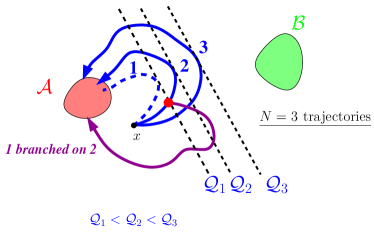
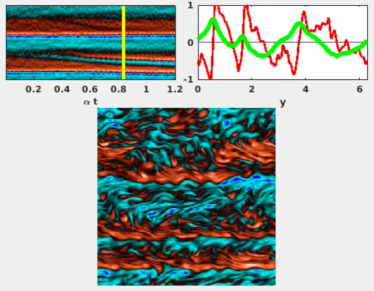
Fig. 4 and the associated movie (Supplementary Video) describe $2\to 3$ transitions for $\alpha=6.0\ 10^{-4}$. Both the movie and the figure clearly illustrate that a new jet formation proceeds through the nucleation of two new ensembles of small positive and negative vortices lying in an area of overall zero vorticity located at a westward jet. Like in condensed matter, such a nucleation is highly improbable. Indeed a too small new vortex band is unstable. However when exceptionally, by chance, a critical size is reached the new band becomes stable and will last for an extremely long time. In combination with this growth, the three jets move apart. It is striking to note that all nucleations ($2\rightarrow 3$ transitions) have been observed at the edge of westward jets, and all coalescences ($3\rightarrow 2$ transitions) occurred at the edge of eastward jets. This phenomenology is illustrated on an even clearer way on Fig. 5 (a) that shows a typical zonal velocity evolution during the nucleation of new jet and Fig. 5 (b) that shows jet coalescence.

(a)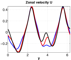

(b)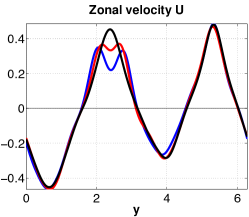

Figure 5: (a) Zonally averaged velocity during the nucleation of a third jet in a $2\to 3$ jet transition: The blue, red and black curves show the velocity field at the start, at an intermediate stage, and at a more advanced stage of the nucleation, respectively. (b) Zonally averaged velocity during the coalescence of two jets in a $3\to 2$ transition: The blue, red and black curves show the velocity field before, just before, and after the merging, respectively. These 4 plots illustrate that while transitions appear at random time, their dynamic is predictable.

The Arrhenius law, from thermodynamics and statistical physics, states that transitions rates are proportional to $\lambda\propto\exp(-\Delta V/\alpha)$, where $\Delta V$ is either a free energy, an entropy, or a potential difference, and $\alpha$ is related to thermal or non-thermal noises. This classical law describes transitions in many fields of physics, chemistry, biology, statistical and quantum mechanics. Could it be relevant to turbulence problems, extremely far from equilibrium? This fascinating hypothesis has never been tested for turbulent flows because this requires a huge number of rare transitions for different values of $\alpha$, an impossible task without a rare event algorithm. The validity of this hypothesis is suggested by the nucleation phenomenology. Moreover, we have recently conjectured Bouchet et al. (2013, 2018) that the slow evolution of the zonally averaged part of the flow, $U(y,t)=\int\mbox{d}x\,\mathbf{v}(x,y,t)$, may be described by an effective equation

$$\frac{\partial U}{\partial\tau}=F(U)+\sqrt{\alpha}\sigma(U,\tau),$$ (2)

where $\tau=\alpha t$ is a rescaled time, $F(U)$, the average of the divergence of the Reynolds stress (more precisely, Bouchet et al. (2013) derived Eq. (2) formally and proved that the hypothesis for the asymptotic expansion leading to $F(U)$ are self-consistent, while Bouchet et al. (2018) explained how to compute $\sigma(U,\tau))$). The classical Freidlin–Wentzell theory Freidlin and Wentzell (1984) describes large deviations and rare transitions for Eq. (2) for weak noises ($\alpha\ll 1$). From this theory, two main consequences can be derived from Eq. (2): first an Arrhenius law, and second a concentration of transition paths close to a single path called instanton Bouchet et al. (2016); Grafke et al. (2017, 2015) (see Berhanu et al. (2007) for an experimental observation in a magneto hydrodynamics turbulent flow, and Grafke et al. (2015) for numerical results for Burger’s equation). In the following of this letter we will show that these two consequences are verified, giving further support to Eq. (2).

Figure 6: Instantons: The reactive tubes corresponding to the distribution of transition paths for the $2\to 3$ (red) and $3\to 2$ (blue) transitions. They illustrate the concentration of transition paths typical of an instanton phenomenology (see the main text) ($\beta=5.26$ and $\alpha=1.2\cdot 10^{-3}$).

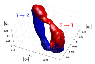
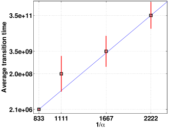
Using the adaptive multilevel splitting algorithm, we have been able to collect thousands of transition paths. In Fig. 6, $80\%$ of the direct $2\to 3$ transitions are inside the red tube, and $80\%$ of the direct $3\to 2$ trajectories are inside the blue tube, in the reduced space of observables $\left(\left|q_{2}\right|,\left|q_{3}\right|,\left|q_{4}\right|\right)$ (see Fig. 2). This unambiguously illustrates the concentration of transition paths close to an instanton. This is the first demonstration of such a phenomenology from numerical simulations in a turbulent flow. We stress the strong asymmetry between the $2\to 3$ and $3\to 2$ transition, which is expected for an irreversible dynamics of a turbulent flow. We also study for the first time in a turbulent flow an Arrhenius law, based on thousands of extremely rare transitions (see Tab. 1). Following the approach described in Cérou et al. (2011) we compute the averaged transition time $\mathbb{E}(T)=1/\lambda$ for the $2\rightarrow 3$ transitions (see Fig. 7). Those data are clearly compatible with an Arrhenius law $\log\mathbb{E}(T)\propto\Delta V/\alpha$. Viscosity effects are discussed in the Supplementary Material file.

Figure 7: Arrhenius law. Logarithm of the mean first transition time $T$ from the two-jet to the three-jet attractors versus $1/\alpha$ ($\beta=5.5$). This result suggests that mean transition times might follow an Arrhenius law $T\propto\text{e}^{\Delta U/\alpha}$. (b)

$\alpha$	AMS	DNS
$1.2\cdot 10^{-3}$	1.0d	15d
$0.9\cdot 10^{-3}$	1.4d	210d
$0.6\cdot 10^{-3}$	2.2d	$\sim$51y
$0.45\cdot 10^{-3}$	3.4d	$\sim$2050y

Table 1: CPU time (d: days, y: years) needed to obtain 1000 transition paths using 200 processors for the adaptive multilevel splitting algorithm compared to direct numerical simulation for different values of $\alpha$.

The new use of the adaptive multilevel splitting algorithm for studying rare transitions in a turbulent flow demonstrates for the first time that thousands of vortices can self-organize and nucleate new structures and trigger transitions. Like in condensed matter, the transition paths concentrate close to instantons. Instantons may be used as precursors stressing that the extremely rare transition became more probable. A very important future work will be the study of Jupiter’s abrupt climate changes with models that are more realistic then the barotropic $\beta$-plane model Schneider and Liu (2009). While it is unlikely that the same nucleation phenomenology should hold for all possible turbulent transitions, the methodology developed will prove useful to study many other transitions related to drastic changes for climate, geophysical, astrophysical and engineering applications. This opens a new range of studies impossible so far, and bring turbulent phenomena in the realm of non-equilibrium statistical mechanics. Examples include the Kuroshio current bistability, weather regime changes in meteorology, regime transitions in the Sun superficial dynamics, astrophysical magnetic field transitions, bistability in turbulent boundary layer detachments.

I Supplementary Materials for the letter: A rare event algorithm links transitions in turbulent flows with activated nucleations, by F. Bouchet, J. Rolland and E. Simonnet

The beta-plane model for barotropic flows.

All the results in this letter are based on the barotropic quasi-geostrophic equations, with a beta plane approximation for the variation of the Coriolis parameter. The equations in a doubly periodic domain $\mathcal{D}=[0,2\pi Ll_{x})\times[0,2\pi L)$ read

$$\partial_{t}\omega+\mathbf{v}\cdot\mathbf{\nabla}\omega+\beta_{d}v_{y}=-\lambda_{f}\omega-\nu_{n,d}\left(-\Delta\right)^{n}\omega+\sqrt{\sigma}\eta,$$ (3)

where $\mathbf{v}=\mathbf{e}_{z}\times\mathbf{\nabla}\psi$ is the non-divergent velocity, $v_{y}$ the meridional velocity component, $\omega=\Delta\psi$ and $\psi$ are the vorticity and the stream function, respectively. $\lambda_{f}$ is a linear friction coefficient, $\nu_{n,d}$ is a (hyper-)viscosity coefficient, and $\beta_{d}$ is the mean gradient of potential vorticity. $\eta$ is a white in time Gaussian random noise, with spatial correlations

$$\mathbf{E}\left[\eta({\bf r}_{1},t_{1})\eta({\bf r}_{2},t_{2})\right]=C({\bf r}_{1}-{\bf r}_{2})\delta(t_{1}-t_{2})$$

that parameterizes the curl of the forces (physically due, for example, to the effect of baroclinic instabilities or convection). The correlation function $C$ is assumed to be normalized such that $\sigma$ represents the average energy injection rate, so that the average energy injection rate per unit of area (or equivalently per unit of mass taking into account density and the layer thickness) is $\epsilon=\sigma/4\pi^{2}L^{2}l_{x}$. These equations share the mathematical properties of the 2D Navier–Stokes equations and reduce to it when $\beta=0$.

The dynamics of large scale jet formation on Jupiter may be qualitatively well understood within the framework of the barotropic quasi-geostrophic equations with a $\beta$ plane approximation, although more refined models are needed to understand their quantitative features Schneider and Liu (2009). As the aim of this work is to make progress in the theoretical understanding of turbulent flows, we consider the simple barotropic $\beta$ plane model. Despite all its limitations, for instance the lack of dynamical effects related to baroclinic instabilities, this model reproduces the main qualitative features of the velocity profile and of the jet spacing. The aim of this study is to make a first study of rare transitions for genuine turbulent flows which is directly inspired by geophysical phenomena, rather than studying precisely specific geophysical phenomena.

For atmospheric flows, viscosity is often negligible in the global energy balance and this is the regime that we will study in the following. Then the main energy dissipation mechanism is linear friction. The evolution of the average energy (averaged over the noise realizations) $E$ is given by

$$\frac{dE}{dt}=-2\lambda_{f}E+\sigma.$$

In a stationary state we have $E=E_{stat}=\sigma/2\lambda_{f}$, expressing the balance between forces and dissipation. This relation gives the typical velocity associated with the coherent structure $U\sim\sqrt{E_{stat}}/L\sim\sqrt{\epsilon/2\lambda_{f}}$. We expect the non-zonal velocity perturbation to follow an inviscid relaxation, on a typical time scale related to the inverse of the shear rate $U/L$. Assuming that a typical vorticity or shear is of order $s=U/L$ corresponding to a time $\tau=L/U$, it is then natural to define a non-dimensional parameter $\alpha$ as the ratio of the shear time scale over the dissipative time scale $1/\lambda_{f}$,

$$\alpha=\lambda_{f}\tau=L\sqrt{\frac{2\lambda_{f}^{3}}{\epsilon}}.$$

When $\beta$ is large enough, several zonal jets can develop in the domain. An important scale is the so-called Rhines scale $L_{R}$ which gives the typical size of the meridional jet width:

$$L_{R}=\left(U/\beta_{d}\right)^{1/2}=\left(\epsilon/\beta_{d}^{2}\lambda_{f}\right)^{1/4}.$$

We write the non-dimensional barotropic equation using the box size $L$ as a length unit and the inverse of a typical shear $\tau=L/U$ as a time unit. We thus obtain (with a slight abuse of notation, due to the fact that we use the same symbols for the non-dimensional fields):

$$\partial_{t}\omega+\mathbf{v}\cdot\mathbf{\nabla}\omega+\beta v_{y}=-\alpha\omega-\nu_{n}\left(-\Delta\right)^{n}\omega+\sqrt{2\alpha}\eta,$$ (4)

where, in terms of the dimensional parameters, we have $\nu_{n}=\nu_{n,d}\tau/L^{2n}$, $\beta=\beta_{d}L\tau$. Observe that the above equation is defined on a domain $\mathcal{D}=[0,2\pi l_{x})\times[0,2\pi)$ and the averaged stationary energy for $\nu_{n}\ll\alpha$ is of order one. Moreover the non dimensional number $\beta$ is equal to the square of the ratio of the domain size divided by the Rhines scale. As a consequence, according to empirical observations in numerical simulations, the number of jets approximately scales like $\beta^{1/2}$ when $\beta$ is changed Dritschel and McIntyre (2008). We are interested in the strong jet regime, obtained for small values of $\alpha$, which is relevant for Jupiter. All the computations of this paper are performed with the parameters $\nu=1.5\ 10^{-8}$, and using a stochastic force with a uniform spectrum in the wave number band $|k|\in[14,15]$. We change the values of $\alpha$ and $\beta$ for different experiments, as explained in the letter.

The adaptive multilevel splitting algorithm and its validation.

The sketch and caption of Fig. 3 explain the principle of the adaptive multilevel splitting algorithm. The cloning step for the discretization of a continuous time dynamics has to be more precisely defined. We denote $1$ the deleted trajectory, $1^{\prime}$ the new trajectory, and $2$ the trajectory used for branching. $X_{1}(t)$ and $X_{2}(t)$ are the values of the model variables along the trajectories $1$ and $2$, respectively. The new trajectory $1^{\prime}$ is equal to the trajectory $2$ up to the first time step $t_{c}$ such that $\mathcal{Q}(X_{2}(t_{c}))>\max_{t}\mathcal{Q}(X_{1}(t))$ Bréhier et al. (2015). In the case of a discrete time process, the branching level must therefore occurs at a discrete time strictly larger than $t_{c}$. Trajectory 1’ is then computed as a numerical solution of (4), with a new realization of the noise $\eta(t)$ for times larger than $t_{c}$ (we recall that $\eta$ is a random Gaussian field with two-point correlation function $C$; a new realization is a new sample of this random field). Any other branching choice adds a bias on the computed transition times. After $K$ iterations, the probability of the set of $N$ selected trajectories is $(1-1/N)^{K}$. If the user chooses to stop the algorithm at the iteration $K$ when $N$ trajectories reach the set $\mathcal{B}$, he obtains a set of $N$ reactive trajectories, which probability is $p=(1-1/N)^{K}$. The averaged transition time is estimated as $\mathbb{E}(T)=\left(\frac{1}{p}-1\right)E_{a}+E_{b}$. The quantity $E_{a}$ is the averaged time to go from the boundary $\partial{\cal A}$ of the set ${\cal A}$ to some hypersurface $\partial{\cal C}$ close to $\partial{\cal A}$ and going back to ${\cal A}$ without going to ${\cal B}$. This quantity is easily estimated by direct simulations since $\partial{\cal C}$ must be close to $\partial{\cal A}$, The quantity $E_{b}$ is the averaged time to go from ${\cal A}$ to $\partial{\cal C}$ and then to ${\cal B}$ without first going back to ${\cal A}$. The conditions under which this approximation is correct, and a justification, are discussed in details in Cérou et al. (2011).

A necessary condition for the adaptive multilevel algorithm to be efficient is to have a good choice of the score function $\mathcal{Q}$ (see Fig. 3). The optimal choice for $\mathcal{Q}$ is the probability to reach the attractor $\mathcal{B}$ before reaching the attractor $\mathcal{A}$ (the committor function). This committor function is however unknown. The choice of $\mathcal{Q}$ should then be made based on heuristic understanding of the transition dynamics. A bad choice of $\mathcal{Q}$ can lead to the failure of the algorithm to efficiently produce reactive trajectories, which is immediately noticed by the user. A more subtle possible difficulty may occur when several sets of transitions paths exists (bistability for the transition paths, in the path space). Then several different score functions should be used in order to compute independently different sets of transition paths.

The reduced phase space is spanned by the moduli of the zonal Fourier coefficients $q_{n}=\int\mbox{d}x\mbox{d}y\,\omega(x,y)\mbox{e}^{iny}/(2\pi)^{2}$ (see Fig 2), with $n=2$, $n=3$ and $n=4$. We first approximate their probability density functions (PDFs) by monitoring $\left|q_{2}\right|$, $\left|q_{3}\right|$ and $\left|q_{4}\right|$ by direct numerical simulation. The sets $\mathcal{A}$ and $\mathcal{B}$ (see Fig. 3) correspond to some low-dimensional projections of the metastable states having two and three eastern jets respectively, for some range of values of $\left|q_{2}\right|$, $\left|q_{3}\right|$ and $\left|q_{4}\right|$ . This procedure defines two sets with disjoint compact support. The support of $\mathcal{A}$ is inside the region $|q_{2}|\in[0.24,0.25],$ $|q_{3}|,|q_{4}|\in[0,0.05]$. The support of $\mathcal{B}$ is inside a larger region $|q_{2}|\in[0.1,0.15]$, $|q_{3}|\in[0.20,0.30]$ and $|q_{4}|\in[0.1,0.2]$. We denote $\mathbf{M}$ a given point in the reduced phase space with coordinates $|q_{2}|,|q_{3}|,|q_{4}|$, and we define the reactive coordinate $\mathcal{Q}$ as $\mathcal{Q}(\mathbf{M})=d_{\mathcal{A}}/2d_{\mathcal{B}}$ if $d_{\mathcal{A}}<d_{\mathcal{B}}$, $\mathcal{Q}(\mathbf{M})=1-d_{\mathcal{B}}/2d_{\mathcal{A}}$ if $d_{\mathcal{A}}>d_{\mathcal{B}}$, and $\mathcal{Q}(\mathbf{M})=1/2$ if $d_{\mathcal{A}}=d_{\mathcal{B}}$; where $d_{{C}}={\rm dist}(\mathbf{M},{C})$. The function $\mathcal{Q}$ is thus equal to zero in the set $\mathcal{A}$ and one in the set $\mathcal{B}$. This choice for $\mathcal{Q}$ is a very rough approximation of the committor isosurfaces but gives rather good results with the adaptive multilevel splitting algorithm as demonstrated in this letter.

For $\alpha=1.2\cdot 10^{-3}$, the only $\alpha$ value for which transitions can be observed using direct numerical simulations, we have verified that the transition paths obtained using the adaptive multilevel splitting algorithm are qualitatively similar to the ones observed in the direct numerical simulations. As seen on Fig. 2, from the direct numerical simulation, only five $2\to 3$ and five $3\to 2$ transitions have been observed. The time spent in the two jet and three jet state is about $2.7\ 10^{6}$ and $2.1\ 10^{6}$ respectively over a total of $4.8\ 10^{6}$. This gives an extremely rough estimate of the average transition time of order of $5.3\ 10^{5}$ for the $2\to 3$ transition and $4.3\ 10^{5}$ for the $3\to 2$ transitions, respectively. As only 5 transitions have been observed, the uncertainty of this estimate is huge, probably of about the same order of magnitude as the estimate itself. Using the adaptive multilevel splitting algorithm for the same parameters, with $N=1000$ clones for each realization of the algorithm, and three realizations of the algorithm, we obtain an estimate of the average transition time of $T\simeq 5.8\cdot 10^{5}$ for the $2\to 3$. This is clearly compatible with what is observed in the direct numerical simulation. We thus conclude that there is a good qualitative agreement between the direct numerical simulations and the adaptive multilevel splitting. A more quantitative agreement can not be checked directly due to the prohibitive cost of direct numerical simulations, but has been checked in models like the stochastic Allen–Cahn equation Rolland et al. (2016), for which explicit mathematical formula were available as a benchmark.

A remark about the instanton shape and the 3 jet attractor.

On Fig. 6, the red tube is a level set of the distribution of transition paths in the reduced space $(|q_{2}|,|q_{3}|,|q_{4}|)$ for the $2\to 3$ transition. It illustrates the concentration of transition paths typical of an instanton phenomenology. The blue tube is the same for the $3\to 2$ transitions ($\beta=5.26$ and $\alpha=1.2\cdot 10^{-3}$). In the Freidlin-Wentzell theory, for an irreversible dynamics like the Navier–Stokes equations and for a classical phenomenology with two attractors separated by a saddle point, one expects the transition paths to form a figure eight. This is not observed on Fig. 6. One can also note on Fig. 6, the large extension of the three jet attractor, related to the fact that the observable $q_{3}$ has strong fluctuations for the three jet state, as can be seen on Fig. 2. Those fluctuations are associated to the fact that for this value of $\beta$, the three jet state is often asymmetric. For instance on Fig. 2, for $550<\alpha t<1150$, one clearly sees that two of the areas with negative values of the vorticity (color blue), are smaller than the third. The extent of this asymmetry changes in time, sometimes fast, sometimes very slowly, suggesting a complex internal dynamics of the three jet attractor. We believe that the absence of a figure height for the transition paths and this apparently complex dynamics in the neighborhood of the three jet attractor are deeply connected. A more precise explanation requires a new study of the three jet attractor which will be the subject of future works.

Hyperviscosity and the Arrhenius law.

Fig. 7 features the logarithm of the transition time versus $1/\alpha$. We note that for $1/\alpha=4\,500$, we have obtained a value of the transition time lower than what should be expected according to the Arrhenius law, by a factor of about two. We have also noticed that for such small values of $\alpha$, hyperviscosity affects consequently the energy balance, suggesting that hyperviscosity is too large for reaching the zero hyperviscosity asymptotical regime. Lowering the hyperviscosity would however require to use a better resolution for the numerical simulation and represent a very subsequent numerical effort that goes beyond the scope of this letter. Given these elements, we conclude that while our results are compatible with the validity of an Arrhenius law, a definitive numerical evidence of the validity of an Arrhenius law would require better resolved numerical simulations.

References

- Sommeria (1986) J. Sommeria, J. Fluid Mech. 170, 139 (1986).
- Ravelet et al. (2004) F. Ravelet, L. Marié, A. Chiffaudel, and F. Daviaud, Phys. Rev. Lett. 93, 164501 (2004).
- Berhanu et al. (2007) M. Berhanu, R. Monchaux, S. Fauve, N. Mordant, F. Pétrélis, A. Chiffaudel, F. Daviaud, B. Dubrulle, L. Marié, F. Ravelet, M. Bourgoin, P. Odier, J.-F. Pinton, and R. Volk, Eur. Phys. Lett. 77, 59001 (2007).
- Wei et al. (2015) P. Wei, S. Weiss, and G. Ahlers, Phys. Rev. Lett. 114, 114506 (2015).
- Zimmerman et al. (2011) D. S. Zimmerman, S. A. Triana, and D. P. Lathrop, Phys. Fluids 23, 065104 (2011).
- Huisman et al. (2014) S. G. Huisman, R. C. van der Veen, C. Sun, and D. Lohse, Nat. comm. 5 (2014).
- Pomeau (2016) Y. Pomeau, Nature Physics 12, 198 (2016).
- Barkley et al. (2015) D. Barkley, B. Song, V. Mukund, G. Lemoult, M. Avila, and B. Hof, Nature 526, 550 (2015).
- Shih et al. (2015) H.-Y. Shih, T.-L. Hsieh, and N. Goldenfeld, Nat. Phys. 12, 245 (2015).
- Rahmstorf et al. (2002) S. Rahmstorf et al., Nature 419, 207 (2002).
- Rogers (1995) J. Rogers, The Giant Planet Jupiter, Practical Astronomy Handbooks (Cambridge University Press, 1995).
- Marcus (2004) P. S. Marcus, Nature 428, 828 (2004).
- Vallis and Maltrud (1992) G. Vallis and M. E. Maltrud, J. Phys. Oceanogr. 23, 1346 (1992).
- Dritschel and McIntyre (2008) D. G. Dritschel and M. E. McIntyre, J. Atmos. Sci. 65, 855 (2008).
- Galperin et al. (2001) B. Galperin, S. Sukoriansky, and H.-P. Huang, Phys. Fluids 13, 1545 (2001).
- Farrell and Ioannou (2007) B. F. Farrell and P. J. Ioannou, J. Atmos. Sci. 64, 3652 (2007).
- Tobias and Marston (2013) S. Tobias and J. Marston, Phys. Rev. Lett. 110, 104502 (2013).
- Srinivasan and Young (2011) K. Srinivasan and W. R. Young, J. Atmos. Sci. 69, 1633 (2011).
- Bouchet and Simonnet (2009) F. Bouchet and E. Simonnet, Phys. Rev. Lett. 102, 094504 (2009).
- Laurie et al. (2014) J. Laurie, G. Boffetta, G. Falkovich, I. Kolokolov, and V. Lebedev, Phys. Rev. Lett. 113, 254503 (2014).
- Kolokolov and Lebedev (2016a) I. Kolokolov and V. Lebedev, Phys. Rev. E 93, 033104 (2016a).
- Kolokolov and Lebedev (2016b) I. Kolokolov and V. Lebedev, J. Fluid Mech. 809 (2016b).
- Woillez and Bouchet (2017) E. Woillez and F. Bouchet, EPL 118, 54002 (2017).
- Bouchet et al. (2016) F. Bouchet, C. Nardini, and T. Tangarife, in 5th Warsaw School of Statistical Physics (2016) p. 34.
- Cérou and Guyader (2007) F. Cérou and A. Guyader, Stoch. Anal. and Appl. 25, 417 (2007).
- Bréhier et al. (2015) C.-E. Bréhier, T. Lelièvre, and M. Rousset, ESAIM: Probability and Statistics 19, 361 (2015).
- Rolland et al. (2016) J. Rolland, F. Bouchet, and E. Simonnet, J. Stat. Phys. 162, 277 (2016).
- Cérou and Guyader (2016) F. Cérou and A. Guyader, Ann. Appl. Probab. 26, 3319 (2016).
- Bouchet et al. (2013) F. Bouchet, C. Nardini, and T. Tangarife, J. Stat. Phys. 153, 572 (2013).
- Bouchet et al. (2018) F. Bouchet, J. Marston, and T. Tangarife, Phys. Fluids 30, 015110 (2018).
- Freidlin and Wentzell (1984) M. I. Freidlin and A. D. Wentzell, Random perturbations of dynamical systems (Springer - New York, Berlin, 1984).
- Grafke et al. (2017) T. Grafke, T. Schäfer, and E. Vanden-Eijnden, in Recent Progress and Modern Challenges in Applied Mathematics, Modeling and Computational Science (Springer, 2017) pp. 17–55.
- Grafke et al. (2015) T. Grafke, R. Grauer, and T. Schäfer, J. Phys. A: Math. and Theoret. 48, 333001 (2015).
- Cérou et al. (2011) F. Cérou, A. Guyader, T. Lelièvre, and D. Pommier, J. of Chem. Phys. 134, 054108 (2011).
- Schneider and Liu (2009) T. Schneider and J. Liu, J. Atmos. Sci. 66, 579 (2009).
Acknowledgments
The authors thank Corentin Herbert, Eric Vanden-Eijnden and Tobias
Grafke for useful discussions. The research leading to these results
has received funding from the European Research Council under the
European Union’s seventh Framework Program (FP7/2007-2013
Grant Agreement No. 616811) (F. Bouchet). All three authors have equally contributed to the research and writing
of this letter.
This submission contains a Supplementary Material file and a Supplementary Video that features an extremely
rare nucleation of a new jet. Such a process has never been observed
before.
Please see next page for the Supplementary Materials.