Imprints of the first billion years: Lyman limit systems at
Abstract
Lyman Limit systems (LLSs) trace the low-density circumgalactic medium and the most dense regions of the intergalactic medium, so their number density and evolution at high redshift, just after reionisation, are important to constrain. We present a survey for LLSs at high redshifts, –5.4, in the homogeneous dataset of 153 optical quasar spectra at from the Giant Gemini GMOS survey. Our analysis includes detailed investigation of survey biases using mock spectra which provide important corrections to the raw measurements. We estimate the incidence of LLSs per unit redshift at to be . Combining our results with previous surveys at , the best-fit power-law evolution is with and (68% confidence intervals). Despite hints in previous results, there is no indication for a deviation from this single power-law soon after reionization. Finally, we integrate our new results with previous surveys of the intergalactic and circumgalactic media to constrain the hydrogen column density distribution function, , over 10 orders of magnitude. The data at are not well described by the model previously reported for –3 (after re-scaling) and a 7-pivot model fitting the full –5 dataset is statistically unacceptable. We conclude that there is significant evolution in the shape of over this 2 billion year period.
keywords:
quasars: absorption lines – cosmological parameters – cosmology: observations1 Introduction
One of the three main classes of H i absorption systems seen along quasar sightlines are the Lyman limit systems (LLSs), caused by hydrogen clouds with integrated H i column densities () large enough to produce optically thick absorption at the Lyman continuum. These clouds are generally highly ionized, with neutral fractions of a few per cent or less (e.g. Steidel, 1990; Prochaska, 1999; Fumagalli et al., 2016). Their high H i column densities, however, imply an origin in dense environments such as galaxy haloes, tracing accreting, outflowing, and stripped gas, or in the most dense regions of the intergalactic medium (IGM).
The clear observational signature of an LLS is a break at the Lyman limit (LL), i.e. the drop in flux transmission at rest-frame wavelength Å, corresponding to the ionization energy of hydrogen ( eV). The optical depth at this break is a defining characteristic of the population, with the canonical defining limit for a LLS, corresponding to . LLS clouds trace both highly enriched gas, likely ejected into galaxy haloes by AGN or supernovae-driven winds (e.g. Péroux et al., 2006; Prochaska et al., 2006), and also gas with very low enrichment levels (Fumagalli et al., 2011a), which may represent either orphaned pockets of baryons in the IGM that have escaped enrichment by recent star formation, or the accreting gas streams that cosmological simulations predict fuel most star formation in the early Universe (e.g. Fumagalli et al., 2011b; Crighton et al., 2016). The LLS distribution also influences how reionization progresses, by altering the propagation of ionizing photons through the IGM, affecting the morphology of ionized bubbles and the measured 21cm correlation signal (Shukla et al., 2016). An empirical estimation of their incidence, therefore, constrains the processes of reionization and also informs models describing the accretion of cool gas onto galaxies (e.g. Fumagalli et al., 2011b; Faucher-Giguère & Kereš, 2011).
Since the first statistical measurement of the LLS incidence by Tytler (1982), with the number of LLSs that occur at random in an interval , there have been many measurements of the LLS distribution (e.g. Sargent et al., 1989; Lanzetta, 1991; Stengler-Larrea et al., 1995). The most recent use large samples of quasars over narrow redshift ranges, and extensively quantify systematic effects with mock observations. Prochaska et al. (2010) measure with a sample of 429 quasars at from the Sloan Digital Sky Survey (SDSS). Ribaudo et al. (2011) and O’Meara et al. (2013) assemble a combined sample of 317 quasars to measure at , and Fumagalli et al. (2013) make a measurement at with a survey of 61 quasars. Ribaudo et al. (2011) showed that the evolution in the incidence rate of systems can be modelled by a power law with .
Of generally greater physical interest is the quantity with defined so that is invariant if the product of the average physical size and comoving number density of the LLS population is constant (see section 3 of Bahcall & Peebles, 1969). Fumagalli et al. (2013) reported strong evolution in for LLSs with cosmic time and introduced a physically-motivated toy model assuming LLSs are produced in the haloes of galaxies in a redshift-dependent way. They find that a model where LLSs arise only in haloes with masses larger than the characteristic mass qualitatively matches the observed evolution in at . Neither of these models predict strong evolution in at higher redshifts but, as the redshift increases towards the epoch of reionization and there are fewer sources of ionizing radiation, we expect the LLS population to increase substantially. Indeed there is some hint in the results that there might be an upturn in at (Fumagalli et al., 2013).
This inference, however, is tempered by the large statistical uncertainties in the measurements. Indeed, whereas the results at lower redshifts are drawn from nearly 1,000 quasar sightlines and hundreds of LLSs, the measurements at high- have been limited by the number of existing high-quality spectra. To date, the combined samples of Peroux et al. (2003), Songaila & Cowie (2010), and Prochaska et al. (2010) form a heterogeneous set of sightlines. In this work we present a new measurement of for LLSs using a homogeneous sample of 153 quasar spectra in the redshift range , the largest LLS survey over this redshift epoch. We quantify systematic errors affecting our measurement by using mock observations, and show that these effects are important, and must be accounted for to enable an accurate measure of . Combining our results with literature measurements, we show that at high redshift follows a power-law extrapolation fitted to the low redshift results. Lastly, we use these new measurements and previous work to constrain the distribution function from .
Throughout this paper we assume a cosmology of km s-1 Mpc-1, and . All distances quoted are comoving unless stated otherwise.
2 Data
The quasar spectra that form the basis of our analysis are drawn from the Giant Gemini GMOS survey of quasars (GGG; Worseck et al., 2014). The GGG survey comprises spectra of 163 quasars selected from the Seventh Data Release of the SDSS (DR7; Abazajian et al., 2009). Only quasars with emission redshifts in the range were surveyed, with a median of . This provides a sample suitable for measuring the mean free path of hydrogen-ionizing photons by averaging the Lyman continuum absorption along many quasar sightlines. For a full description of the data sample, see Worseck et al. (2014).
This quasar redshift range is also suitable for a statistical measure of individual Lyman limit systems: it is above the interval , where the presence of LLSs can bias the inclusion of quasars in the SDSS (Worseck & Prochaska, 2011), but still at low enough redshift that IGM absorption does not prevent the identification of Lyman limit breaks. The spectra cover –Å in the quasar rest-frame through overlapping blue and red wavelength settings of the Gemini Multi-Object Spectrographs (GMOS) on the northern and southern Gemini telescopes. In this work we mainly use spectra from the blue setting, which covers the Lyman limit and Ly forest. The full-width-at-half-maximum (FWHM) resolution for the blue setting is km s-1, and the typical signal-to-noise ratio (S/N) is 20 per Å pixel in the Ly forest at the estimated, unabsorbed continuum.
As described by Worseck et al. (2014), one GGG quasar spectrum has contaminating absorption by a nearby object on the sky and the sky background is therefore poorly estimated. It was removed from our analysis. Another nine of the quasars show broad absorption lines at C iv, N v and/or O vi. Although we may be able to identify LLSs in these spectra, the broad absorption lines may introduce systematic effects which are absent in non-BAL spectra, so these sightlines are also removed from our analysis sample.
Table 1 lists the set of 153 quasars whose GGG spectra were included in the LLS survey. The emission redshifts were carefully estimated by Worseck et al. (2014) and are critical to defining the search path for LLSs, as described in the following section.
| Name | RA | DEC | |||
|---|---|---|---|---|---|
| (deg) | (deg) | ||||
| J0011+1446 | 2.81349 | 14.7672 | 4.970 | 4.3968 | 4.9106 |
| J0040-0915 | 10.22772 | -9.2574 | 4.980 | 4.7870 | 4.9205 |
| J0106+0048 | 16.58017 | 0.8065 | 4.449 | 3.8803 | 4.3947 |
| J0125-1043 | 21.28927 | -10.7169 | 4.498 | 4.2601 | 4.4433 |
| J0210-0018 | 32.67985 | -0.3051 | 4.770 | 4.2037 | 4.7125 |
| J0231-0728 | 37.90688 | -7.4818 | 5.420 | 5.3389 | 5.3561 |
| J0331-0741 | 52.83194 | -7.6953 | 4.734 | 4.3345 | 4.6769 |
| J0338+0021 | 54.62211 | 0.3656 | 5.040 | 4.4435 | 4.9799 |
| J0731+4459 | 112.76304 | 44.9971 | 4.998 | 4.5146 | 4.9383 |
| J0800+3051 | 120.09590 | 30.8503 | 4.676 | 4.3860 | 4.6195 |
| J0807+1328 | 121.81300 | 13.4681 | 4.880 | 4.6647 | 4.8215 |
aDefined for the discovery of LLSs in the GGG spectra. See the text for details.
bDefined to be 3,000km s-1 blueward of to avoid the quasar proximity region.
3 Formalism
Determining the minimum optical depth at the Lyman limit for LLSs, , that can be reliably determined in the GGG spectra is the first stage of defining the LLS survey. A of unity corresponds to a column density cm-2 and flux transmission , while a LLS with (cm-2, ) absorbs almost all the flux at the break. Systems with are generally referred to as partial LLSs (or pLLSs) and are not considered in this paper (see, e.g., Lehner et al., 2014). After assessing the data quality and performing tests on mock spectra ( 4.3), we decided to limit our analysis to LLSs with in this paper. This follows Prochaska et al. (2010) who identified several biases inherent to LLS surveys and concluded that was the limit for robust analysis with low-dispersion data of high- quasars like those in the GGG survey. This limit has the added advantage of matching that used in many other recent measurements at , thereby enabling direct comparison of results. An LLS with , corresponds to cm-2 and .
The survey aim, then, is to measure the incidence rate of LLSs, . That these systems absorb at least of the flux at their Lyman break makes them straightforward to identify, but it also hinders the identification of lower-redshift LLSs in the same spectrum: the search path for LLSs is effectively cut short by the highest-redshift LLS removing flux at wavelengths shorter than its rest-frame Å. As a result, each observed LLS modifies the total search path of the survey. Previous work has shown (Tytler, 1982; Bechtold et al., 1984) that for a LLS survey of quasars containing LLSs the maximum likelihood estimator for the incidence rate, , is then
| (1) |
where and are the lowest and highest redshifts in the th quasar spectrum where a LLS can in principle be identified. When a Lyman limit system cuts short the search path, then that LLS must be included in the resulting modified search path, i.e. . The denominator represents the integrated redshift path of the survey where a LLS could be detected, often referred to as . Equation 1 is generally evaluated in bins of redshift and one defines , the sensitivity function, as the number of quasar sightlines that may be searched for LLSs at a given redshift. It follows that with the integral performed over a redshift bin.
To separate the effects of cosmological expansion from any evolution in the intrinsic properties of LLSs, we convert the incidence rate as a function of redshift to an incidence rate as a function of absorption distance (see e.g. Bahcall & Peebles 1969), given by
| (2) |
where is the Hubble parameter. The resulting incidence rate is then
| (3) |
4 Analysis
There are two main steps required to measure . The first is to identify and characterize each LLS in the GGG spectra by strength () and redshift (). The second is to define the redshift path for detecting LLSs by evaluating . These steps are done independently although, as emphasized above, any LLSs discovered modify the final search path used in the analysis. In addition, for the LLS survey by Prochaska et al. (2010), which used SDSS spectra covering a lower redshift range than our GGG spectra, important systematics were found that could bias by as much as %. We expect that similar systematics, especially the ‘blending bias’, which we describe in more detail in the following sections, are also present in our GGG survey. In this section we first describe our method for identifying LLSs, and follow with our method for measuring the redshift path. Finally, we describe the set of simulated spectra that we use to quantify systematics, and to find the correction factor from our measured , , to the true .
4.1 LLS identification
LLSs were identified in each quasar spectrum by eye, using a custom-written tool111See the pyigm_fitlls script in the pyigm repository, https://pyigm.readthedocs.io/en/latest.. This tool enables a continuum template to be scaled to an appropriate level above the IGM absorption in the sightline, and for LLSs to be overlaid on the continuum and compared to the data. This by-eye approach is driven by the fact that systematics dominate uncertainty in the analysis, particularly those due to (i) variations in continuum shape and normalization; and (ii) stochastic line-blending with the Ly forest. In future works, we intend to implement machine-learning techniques to perform the analysis on future, large datasets (e.g. Garnett et al., 2017; Parks et al., 2018).
For each sightline, we identified LLSs using the following steps:
-
1.
Estimate the quasar continuum level at wavelengths slightly longer than the quasar Lyman limit. We used a template including IGM absorption, constructed by averaging all quasars in the sample (see below), normalised such that it was just above the highest flux transmission peaks at – Å.
-
2.
Identify the highest redshift, LL candidate, which appears as a break in the continuum shortwards of the quasar Lyman limit. Insert a model for the optical depth for this system into the template continuum. Check the Ly and other Lyman series lines for the system, adjusting its redshift to improve agreement with these lines.
-
3.
Alter until the model matches the observed drop in flux at the absorber’s Lyman limit.
-
4.
Adjust the Doppler broadening parameter () of the absorber to best match the equivalent width of the Lyman series lines.
-
5.
Repeat steps – for all discernable LLSs in the spectrum, moving from the highest to the lowest redshift candidate.
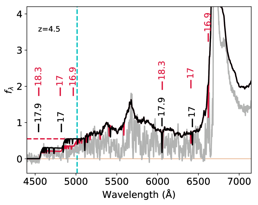
Figure 1 illustrates this process using a mock spectrum (described in Section 4.3).
The continuum template was generated by shifting all of the non-BAL GGG spectra to rest wavelengths, normalising in the rest wavelength range – Å (masking the sky absorption feature at – Å) and averaging them. Below the rest-frame quasar Lyman limit, the presence of Lyman limit systems suppresses the template below the mean IGM flux level, and so we assume a flat continuum in at wavelengths shorter than Å. We did not use metal lines to refine redshifts, because in most cases they were not strong enough to be detected at the S/N and resolution of our spectra.
Inevitably there are some subjective criteria that determine whether a drop in flux in a quasar spectrum is flagged as a LLS. Therefore two of the authors (NC and JO) each identified LLS in every GGG spectrum, enabling us to assess how the identification criteria described above affect the recovered LLS statistics. As an initial validation of our search procedure, we searched for LLSs in a smaller sample of eight spectra before starting the full search. These eight spectra were selected from the real GGG spectra to show no strong Lyman limit absorption within of the quasar Lyman limit, and thus create a set of diverse strong absoprtion-free continua. Between zero and two synthetic LLSs were then inserted into each spectrum, with their and redshift values drawn at random in the ranges cm-2, , and with set to km s-1. Each author searched these spectra for LLSs, and we compared the recovered LLS parameters (, ) with the known parameters. This test showed that in most cases the LLS were recovered correctly, with and redshift close to the known values. We therefore concluded that our search method was sound, and continued fitting all the spectra using these criteria. In Section 4.3 we describe more quantitatively how well our search method recovers systems. Table 2 lists all of the LLSs identified in the full sample by NC. The final set of LLSs used to estimate is drawn from this list.
| RA | DEC | |||
|---|---|---|---|---|
| (deg) | (deg) | (km/s) | ||
| 10.22772 | -9.2574 | 4.78713 | 17.90 | 40.0 |
| 10.22772 | -9.2574 | 4.97083 | 17.20 | 20.0 |
| 16.58017 | 0.8065 | 4.23517 | 17.35 | 50.0 |
| 16.58017 | 0.8065 | 4.06464 | 17.45 | 20.0 |
| 21.28927 | -10.7169 | 4.18351 | 20.20 | 70.0 |
| 21.28927 | -10.7169 | 4.26017 | 17.30 | 20.0 |
| 21.28927 | -10.7169 | 4.23090 | 17.30 | 20.0 |
| 32.67985 | -0.3051 | 4.55488 | 17.35 | 40.0 |
| 32.67985 | -0.3051 | 4.27720 | 17.15 | 20.0 |
| 37.90688 | -7.4818 | 5.33901 | 19.80 | 60.0 |
| 37.90688 | -7.4818 | 4.88711 | 20.70 | 20.0 |
4.2 Defining the redshift path
We define the redshift path for detecting LLSs in one of our spectra in the following way. The lower limit for the path is determined from the bluest wavelength, [Å], where the smoothed S/N – defined as the flux-to-error ratio smoothed by a 20-pixel boxcar filter – is 2 per pixel. We consider this a reasonable compromise between maximising the available redshift path length and enabling a confident detection of LLSs. The lower limit to the search path for that quasar is then . If the Lyman limit of a LLS caused the S/N to drop below this threshold, then this definition led to the system being excluded from the redshift path, greatly suppressing the number of LLS in the survey. To prevent this artificial effect, we check whether there is an observed LLS with redshift , and where such a system is present we set at the LLS redshift, and include that system in the search path if it has . The upper search limit for the search path, is taken to be km s-1 bluewards of the quasar redshift. This offset is chosen to avoid the proximity zone of the quasar which may be biased by gas clustered around the host galaxy (Hennawi & Prochaska, 2007) and/or the quasar radiation field (Faucher-Giguere et al., 2007).
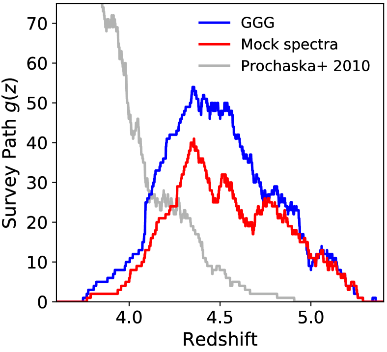
We checked the effect of changing these parameters over reasonable ranges, and found that they do not change the measurement by more than the final error. Table 1 lists the and values for each quasar, and Fig. 2 shows the resulting sensitivity function, . The decline in at follows the decline in the number of quasars in the sample at such redshifts. The decline at , however, is a complex convolution of the GGG quasar redshift distribution, the GGG observing strategy, and the incidence of LLSs which alter .
4.3 Assessment of systematic uncertainties using mock spectra
Our initial check that we could successfully recover LLSs (see Section 4.1) also indicated the presence of systematic errors in the recovered LLS parameters, caused by the low spectral resolution and strong IGM absorption at high redshift. This is not surprising – Prochaska et al. (2010), for example, identified several possible systematic effects introduced when identifying LLSs in SDSS quasar spectra. Their survey used higher resolution, generally noisier spectra, and was at a lower redshift, but we expect many of the systematic effects to also be present in our GGG survey. To assess these systematic errors we generated a sample of mock spectra, one corresponding to each real GGG spectrum, and applied simulated IGM absorption to them. These spectra were then searched for LLSs in the same way as the real spectra by the same two authors (NC and JO). We compared the parameters of LLSs recovered by our search to the known parameters of the LLSs inserted into the mocks to quantify any systematic uncertainties in our LLS identifications. Appendix A discusses our IGM simulations and how we generated the mocks.
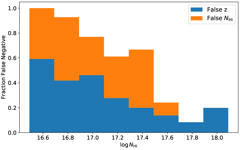
By searching these mock spectra we found that LLSs with could be recovered with high confidence. Fig. 3 shows the incidence fraction of false negatives from the mock analysis with a false negative defined as a true LLS that was mis-identified by the human. We show separately: (i) false negatives in redshift, defined as a true LLS where the nearest human-identified LLS was offset by more than 3,000 km s-1, and (ii) false negatives in , where the estimate value was offset by at least 0.3 dex (where all values were capped at a maximum of 17.8 dex). These are shown as a function of true . The combined false negative rate is 100% for the lowest LLSs injected, i.e. none were correctly recovered. Weaker systems were more difficult to identify, as the relatively shallow depression of flux they produce below the quasar Lyman limit is easy to overlook completely or misinterpret as IGM absorption or quasar continuum fluctuations. The results show further that at cm-2, the rate of false negatives drops markedly.
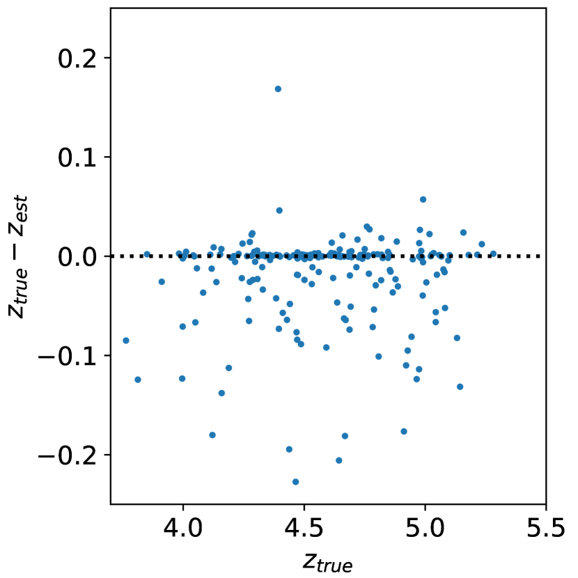
LLSs were most straightforward to identify in quasars with a single, system. More complex sightlines with many, closely-spaced partial LLSs were more difficult to recover accurately. For these complex sightlines, we sometimes identified a single strong LLS to explain the absorption of several lower LLSs, and the redshift difference between the input and recovered LLS could be quite large (). To quantify how well we are able to recover the LLS redshift from the mock spectrum, we take each ‘true’ LLS with in the mocks (described in more detail below) and match it to the nearest guessed LLS in redshift in that spectrum. The results are shown in Fig. 4. For most LLSs, the redshift uncertainty is very small, , but the distribution has broad tails out to . This suggests we can reliably identify strong LLSs, and so make a robust measurement.
4.4 Finding the true
We take the ‘true’ of the mock skewers to be the line density over the redshift range averaged over all quasars. Due to the way we assign LLSs to the simulated skewers (see Appendix A), they often have very small separations, km s-1. In high resolution spectra, LLS components are only judged as belonging to distinct systems if they are separated by more than km s-1 (Prochaska et al., 2015), which is the circular velocity for high mass () dark matter haloes at , and corresponds to the largest range typically observed for metal-lines associated with strong LLSs and DLAs (e.g. Peroux et al., 2003). Therefore, we merge systems with separations less than km s-1, assigning a new redshift given by the mean of the contributing components’ redshifts, weighted by their column densities. This gives the true we compare to the measured values from the mock spectra. The resulting true is not sensitive to the precise merging scale; if we use instead of km s-1, the true changes by less than 2%.
Figure 5 compares derived from the human analysis of the mock spectra with the true evaluation discussed above for . These results suggest that is overestimated by % in the lowest of three redshift bins, and by in the highest redshift bin. By inspecting our fits to the mock spectra and overplotting the known LLS positions (see Fig. 1 for an example), we determined that the main systematic causing this excess is the ‘blending bias’, as described by Prochaska et al. (2010). This refers to the effect from nearby, partial LLSs (with ) that tend to be merged together when identified by their Lyman break alone, and thus are incorrectly identified as a single LLS. This merging occurs due to confusion in identifying the redshift of a LLS: often, all the Lyman series lines have a relatively low equivalent width, and so the only constraint on the LLS redshift is the LL break. The position of the break can be affected by overlapping IGM absorption, and by the velocity structure of the LLS, which is difficult to measure accurately using low-resolution spectra like the GMOS data employed here.
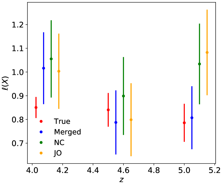
To further illustrate the importance of this systematic effect, we apply a simple merging scheme to the true list of LLSs, and compare for this merged list to our recovered . To do this merging, we step through each LLS with in the true list (described above), from lowest to highest redshift, and test whether there is another system within 9000 km s-1(see below and Fig. 6 for the justification of this value). If one is found, we merge the two systems by adding their column densities, using the redshift of the highest redshift system for the resulting single combined system. This process is repeated, with the new merged system replacing the previous two separate systems, and continued until every system with has been tested in a sightline. corresponds to the optical depth of a LLS which produces an appreciable Lyman break, detectable in the GMOS spectra. Using our mocks, we also explore the effect of setting or 1.5 instead and find that, while it has a negligible effect for the highest and lowest redshift bins in Fig. 5, it can introduce an uncertainty of up to 8% in for the central redshift bin. This is significantly smaller than the final statistical uncertainty on for this bin, but it is large enough that we include its contribution in the final uncertainty budget.
To estimate the merging scale, we measured the distribution of redshift differences between LLSs that we observe towards sightlines showing more than one LLS. Fig. 6 shows these distributions for both authors who identified LLSs. Without the blending bias, one expects a roughly flat distribution at small that then drops with increasing because the presence of one strong LLS precludes the detection of any other at lower . The low number of pairs with , therefore, must be related to the blending bias. We adopt the peak in these distributions as the smallest scale at which we can reliably separate nearby LLSs. The peak for both authors is at , equivalent to 9270 km s-1 at , and we therefore adopt a merging scale of 9000 km s-1. Using a merging scale of 6000 or 12000 km s-1 instead of 9000 km s-1 changes the inferred by less than 3%. Finally, we define a redshift path for this merged list in a similar way for the mock spectra, by truncating the redshift path in a sightline when it encounters a strong LLS.
With this new, merged list of LLSs in the mock spectra, we then make a new measurement of , shown by the blue points in Fig. 5. While these blue points do not precisely match the directly measured values, they do show similar systematic offsets – the first and last bins have an increase in and there is little change in the central bin. We consider this merging effect, which truncates the search path and merges weaker LLSs into systems, to be the main systematic error to correct in our analysis. In the following section we apply the correction derived from this mock spectrum analysis to the real GGG sightlines, and report the final, corrected values.
4.5 measurements
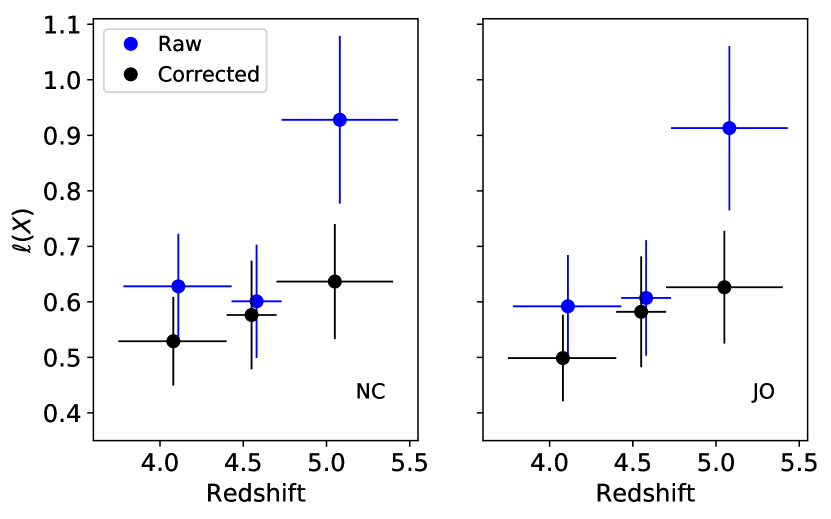
Table 3 lists the final set of LLSs used for the statistical analysis of . We have measured in three redshift bins, –4.4, 4.4–4.7, 4.7–5.4, chosen to have roughly equal numbers of LLSs. The raw measurements from analysis by NC and JO are shown in Figure 7. The two sets of measurements are in excellent agreement; the largest offset is only 4%. We have then corrected these values based on the mock spectrum analysis described in Section 4.4. Table 4 summarizes the measurements including the corresponding values for . We have also estimated across the entire survey () to be .
| RA | DEC | ||
|---|---|---|---|
| (deg) | (deg) | ||
| 10.22772 | -9.2574 | 4.78713 | 17.90 |
| 37.90688 | -7.4818 | 5.33901 | 19.80 |
| 52.83194 | -7.6953 | 4.33463 | 17.80 |
| 112.76304 | 44.9971 | 4.51475 | 17.90 |
| 120.09590 | 30.8503 | 4.38613 | 19.00 |
| 121.81300 | 13.4681 | 4.66482 | 17.80 |
| 125.55146 | 16.0769 | 3.91159 | 19.70 |
| 126.22510 | 13.0381 | 5.02951 | 17.90 |
| 129.23253 | 6.6846 | 4.20632 | 17.90 |
| 129.83555 | 35.4165 | 4.42728 | 18.00 |
| 131.63137 | 24.1857 | 4.50460 | 17.90 |
| Redshift bin | |||||||||||
|---|---|---|---|---|---|---|---|---|---|---|---|
| 3.75–4.40 | 42 | 15.29 | 63.22 | 2.75 | 2.21 | 0.34 | 0.40 | 0.66 | 0.54 | 0.08 | 0.10 |
| 4.40–4.70 | 31 | 13.15 | 56.12 | 2.36 | 2.20 | 0.39 | 0.47 | 0.55 | 0.52 | 0.09 | 0.11 |
| 4.70–5.40 | 36 | 9.28 | 40.89 | 3.88 | 2.95 | 0.49 | 0.58 | 0.88 | 0.67 | 0.11 | 0.13 |
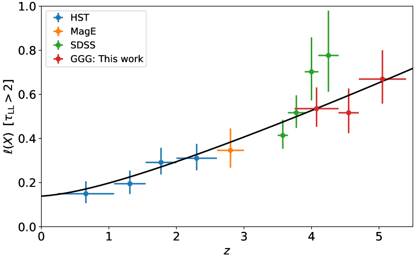
Previous work (e.g. Ribaudo et al., 2011) has shown that measurements are well described by a power-law of the form where is an arbitrary pivot redshift. We compare this model against the combination of our GGG results and the HST datasets of Ribaudo et al. (2011) and O’Meara et al. (2013), the MagE survey by Fumagalli et al. (2013), and the SDSS results from Prochaska et al. (2010)222All of the LLS lists, sensitivity functions, and code to calculate are available in the pyigm repository at https://github.com/pyigm/pyigm .. We adopt the maximum likelihood approach to fitting the LLS surveys, described in Prochaska et al. (2010), and recover and (68% confidence intervals) with . Binned measurements of , assuming binomial statistical uncertainties, are compared against this best-fit model in Fig. 8. We have performed a Kolmogorov–Smirnov test comparing the cumulative distribution function of from the observations and that derived from the convolution of the best-fit and the survey sensitivity functions. We recover an acceptable probability of only 23% that the null hypothesis is ruled out.
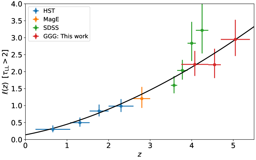
Fig. 9 presents the final measurements for the GGG sample using the results from one author (NC) from Fig. 7. These are shown together with evaluations of for systems from previous, lower redshift measurements. There is no evidence for a sudden change in the LLS incidence rate at –5, which has been speculated about previously (e.g. Fumagalli et al., 2013; Crighton et al., 2015) based on the highest redshift points from the SDSS analysis of Prochaska et al. (2010). Indeed, the two highest redshift bins from the SDSS sample have large uncertainties and are consistent with our results within the combined uncertainties. Furthermore, we suspect a correction for the blending bias should be applied to those SDSS measurements, in a similar fashion performed for the GGG results here.
4.6 Clustering of LLSs
Clustering of LLSs can potentially introduce a systematic effect where the measured significantly underestimates the true . This is because of the survival nature of the measured , where a single LLS in a sightline prevents detecting any lower redshift LLS. Therefore, only the highest redshift component of a cluster of several LLSs is measured. In principle this can suppress by a factor comparable to the number of LLSs per cluster, an effect that has not (to our knowledge) been quantified in previous measurements (as noted by Prochaska et al., 2014, hereafter P14) Indeed, Prochaska et al. (2013) reports a large clustering length-scale Mpc for the LLS–quasar cross-correlation function, suggesting a high degree of clustering near massive haloes. An ongoing survey with pairs of quasar spectra will provide the auto-correlation function for LLSs in a random distribution of environments (Fumagalli et al., in preparation).
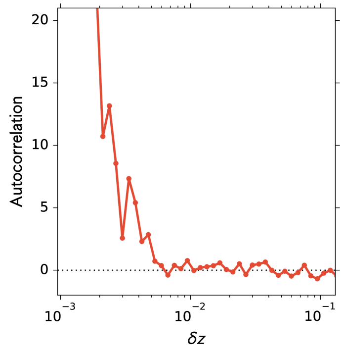
We use our simulated ‘skewers’ (see Appendix A) to estimate the importance of this clustering in the simulated spectra. We measure the autocorrelation of LLSs with in the simulated skewers as a function of redshift separation. The results are shown in Fig. 10. Correlation is only significant at scales (550 km s-1 at ). Since these scales are much less than the merging length described above (9000 km s-1), they imply that clustering will not not have a significant effect on our measured . However, we emphasise that this conclusion should be tested with simulations which more accurately reproduce the distribution of LLSs and include radiative transfer effects.
| Constraint | Value | Reference | |||||
|---|---|---|---|---|---|---|---|
| 4.56 | 11.0 | 22.20 | 2.3 | 2.3 | Worseck+14 | ||
| 4.86 | 11.0 | 15.10 | 1.8 | 1.8 | Worseck+14 | ||
| 5.16 | 11.0 | 10.30 | 1.6 | 1.6 | Worseck+14 | ||
| log | 4.40 | 20.300 | 20.425 | -22.12 | 0.24 | 0.21 | Crighton+15 |
| 20.425 | 20.675 | -22.13 | 0.18 | 0.15 | Crighton+15 | ||
| 20.675 | 21.075 | -22.51 | 0.18 | 0.13 | Crighton+15 | ||
| 21.075 | 21.300 | -22.77 | 0.14 | 0.13 | Crighton+15 | ||
| 21.300 | 21.800 | -23.77 | 0.30 | 0.18 | Crighton+15 | ||
| 4.05 | 11.0 | 22.0 | 0.91 | 0.09 | 0.09 | Becker+13 | |
| 4.15 | 11.0 | 22.0 | 0.98 | 0.10 | 0.10 | Becker+13 | |
| 4.25 | 11.0 | 22.0 | 1.02 | 0.10 | 0.10 | Becker+13 | |
| 4.35 | 11.0 | 22.0 | 1.07 | 0.11 | 0.11 | Becker+13 | |
| 4.45 | 11.0 | 22.0 | 1.13 | 0.11 | 0.11 | Becker+13 | |
| 4.55 | 11.0 | 22.0 | 1.20 | 0.12 | 0.12 | Becker+13 | |
| 4.65 | 11.0 | 22.0 | 1.24 | 0.12 | 0.12 | Becker+13 | |
| 4.75 | 11.0 | 22.0 | 1.42 | 0.14 | 0.14 | Becker+13 | |
| 4.85 | 11.0 | 22.0 | 1.50 | 0.15 | 0.15 | Becker+13 | |
| 4.08 | 17.80 | 0.54 | 0.10 | 0.10 | Crighton+18 | ||
| 4.55 | 17.80 | 0.52 | 0.11 | 0.11 | Crighton+18 | ||
| 5.05 | 17.80 | 0.67 | 0.12 | 0.12 | Crighton+18 |
5 Constraints on the high redshift column density distribution
For a combination of scientific, pragmatic, and historical reasons, we are motivated to utilize the LLS results and previous measurements from the GGG survey (and literature) to derive a first estimate for the frequency distribution at . Scientifically, changes in the shape or normalization of with redshift may offer physical insight into evolution in the IGM, CGM, and ISM of high- galaxies. This holds despite the fact that we have no physical model for and only initial efforts to estimate it within cosmological simulations (e.g. McQuinn et al., 2011; Rahmati et al., 2013; Rahmati et al., 2015; Behrens et al., 2018; Rogers et al., 2018a, b). Our approach to evaluating follows the methodology developed in P14. The mathematical model adopted is a Piecewise Cubic Hermite Interpolating Polynomial evaluated here with the PchipInterpolator algorithm in scipy (v1.0.1)333We caution that this algorithm in scipy has changed at least once in the past two years and therefore the results given here may depend on the precise version of scipy. We will endeavor to update our model in the pyigm package as scpiy evolves.. The model is parameterized by seven “pivots” at specific values. As in P14, we assume redshift evolution in the normalization of , and fix for this first model and pivot at . The number and locations of the pivots correspond to values where the model is likely to be well-constrained by the data (e.g. at cm-2 from LLSs) with additional, “outer” pivots at low and high to bound the model. After some experimentation, the pivot positions were slightly adjusted to yield better results.
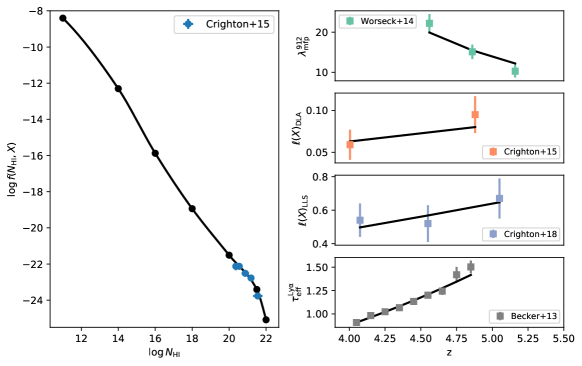
Regarding the observational constraints, we included the following set of measurements, as summarized in Table 5:
-
•
the measurements from Becker et al. (2013) for ;
-
•
the measurements from the GGG survey (Worseck et al., 2014);
-
•
the and measurements of DLAs from the GGG survey (Crighton et al., 2015);
-
•
the measurements from this paper.
Evaluations of to compare against the other, integral constraints were performed with the pyigm package.
We performed a Monte Carlo Markov Chain (MCMC) analysis with the pymc3 (v3.4.1) software package and its “slice sampling” method. We adopted the reported uncertainties for each measurement and assumed a Gaussian distribution in the deviate evaluation. In addition, our final results were derived assuming a Gaussian prior on each pivot within a standard deviation of dex centered on estimates from trial runs. We constructed a set of 8 chains, each with 15000 links modulo a 1,000 step burn-in phase. The collated set of 112,000 links yields the probability density functions describing the function.
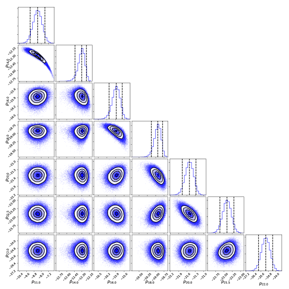
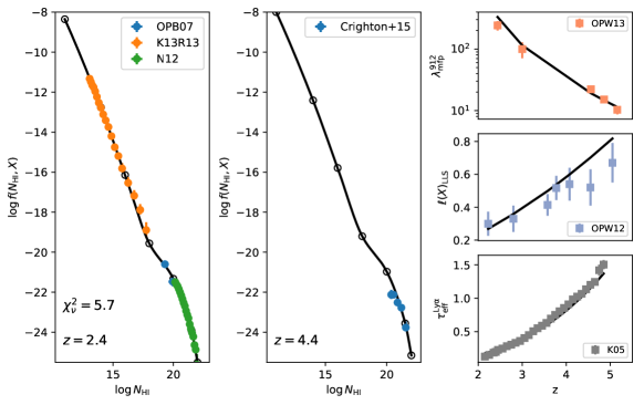
Figure 11 presents the primary results, with the left panel showing the function evaluated at and the right panels comparing the integral constraints against this model. The model provides an excellent description of the integral constraints on and the estimations of in the DLA regime. Uncertainties in the model have been derived from the MCMC chain and are described by the “corner” plots in Figure 12. There is significant correlation between neighbouring points in the model, but the inner pivots are otherwise well-behaved. As should be expected, uncertainties in the outer pivots, used primarily to bound , are the largest. The results are summarized in Table 6 which lists the median normalization of each pivot in the model, at , and the 68% confidence interval from the probability density functions.
| Parameter | Priora | Median | 16th | 84th |
|---|---|---|---|---|
| percentile | percentile | |||
| Results for | ||||
| Results for | ||||
a indicates a Gaussian distribution with mean and standard deviation .
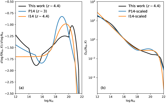
It is clearly evident from Fig. 11 that the distribution is not a single power-law over the 10 orders-of-magnitude in that quasar spectra probe. This is further illustrated in Fig. 13a where we plot against . At cm-2, corresponding to the Ly forest and approximately the mean density of the universe at , and then steepens as increases to cm-2. The distribution then flattens as one enters the optically-thick regime ( cm-2), a behaviour expected in the transition from ionized to neutral gas (e.g. Zheng & Miralda-Escudé, 2002). Figure 13 also compares these results on at with estimates at lower redshifts, –3, based on similar constraints and analysis (Prochaska et al., 2014; Inoue et al., 2014). The behaviour is qualitatively similar between the two models, although the flattening in is more pronounced at . This leads to the bump in for around cm-2, evaluated and shown in Fig. 13b. This bump implies an increase in the relative number of high-column density LLSs and low-column density DLAs from 5 to –3, which at present appears somewhat contrary to predictions from cosmological simulations (e.g. Fumagalli et al., 2011a).
To further examine redshift evolution in the shape of , we have adopted the form of from P14 and derived the most likely value for by fitting to the constraints in Table 5. We derive and the model is compared to the observational constraints in Figure 14. This model greatly over-estimates the incidence of systems (including DLAs) and under-predicts the opacity of the Ly forest. Because modifying the normalization would improve one at the expense of the other, we conclude that the P14 model is a poor description of the observations at .
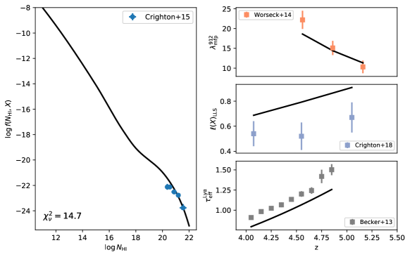
Therefore, we have further generalized the model, combining the 7-pivot model above with a free parameter for . We performed an MCMC analysis with all of the constraints of P14, several additional constraints from the literature, and all of those from Table 5. Figure 15 presents the model compared to the observational data. Qualitatively, the model offers a good approximation to nearly all of the observational constraints at –5. The clear exception is the incidence of DLAs at which is somewhat over-predicted by the model. Similarly, this model systematically overestimates our new measurements for LLS. We also note that the model does not cluster LLS as we have; a proper treatment would likely exacerbate the tension between model and data. Less obvious is the fact that the observational constraints on the measurements and the values for the Ly forest are sufficiently precise that the resultant is large. We report a reduced per degree of freedom in the model, with 74% of the contribution to this coming from the measurements of the Ly forest data. We therefore conclude that the data require evolution in the shape of over the few Gyr from to 2. A similar conclusion was reached by Inoue et al. (2014) at lower redshifts. As emphasized in Fig. 13, the starkest difference in the shapes at and 5 is the additional flattening in the former at cm-2. We encourage further exploration into the CGM and ISM of galaxies in hydrodynamic simulations to further interpret these results. We also note that future work should examine models with an evolving shape to attempt to fully describe the data and understand the reasons for its evolution (see also Inoue et al., 2014).
The other important result from our analysis is which indicates a substantial evolution in the normalization of . A universe where the structures yielding optically thick gas is non-evolving would yield . And given that we expect the number density of structures (e.g. galactic halos) to decrease with increasing redshift (e.g. Fumagalli et al., 2013), this implies an increase in the neutral fraction of such gas (see also Worseck et al., 2014). Furthermore, the fact this holds approximately independent of , implies an increase in the neutral faction of gas on all scales.
6 Conclusions
We have presented LLS survey, drawn from the homogeneous GGG sample of 153 quasar spectra, extending to the highest resshifts to date, –5.4. Using mock spectra to determine the required corrections from the raw LLS counting statistics determined by two different authors, we estimated the incidence of LLSs per unit redshift at 4.4 to be . Breaking the results into 3 redshift bins, and comparing it with previous results from LLS surveys at , we find that the incidence rate decreases with time consistent with a simple power-law in redshift: with and (68% confidence intervals). Our new measurements do not bear out hints for a rapid decline in from 4.2 to 3.6, as hinted at (with relatively large uncertainties) in the LLS survey of SDSS spectra by (Prochaska et al., 2010). That is, we do not detect any clear post-reionization effects in LLS evolution. The simple physical motivation for the power-law evolution described by Fumagalli et al. (2013), in which LLSs only arise in galaxy haloes larger than a characteristic mass, therefore remains a plausible model.
By combining our measurements of the LLS incidence rate with the DLA incidence rate and distribution function (Crighton et al., 2015), and mean-free path measurements (Worseck et al., 2014), from the same GGG spectra, we are able to constrain the shape of the column density distribution function, , below our detection threshold for LLSs ( cm-2). A 7-pivot cubic Hermite interpolating polynomial self-consistently matches these constraints on to measure its normalisation and shape over 10 orders of magnitude, cm-2 – see Fig. 11. However, the previously-reported model of at –3 cannot consistently match the data (allowing for a re-scaling of the normalisation). Nor does a similar model of the combined –5 dataset, with an unevolving shape for , provide a statistically acceptable fit. We are therefore compelled to conclude that the shape of evolves from down to –3. The independent models at these redshifts differ most starkly at column densities around cm-2, so we encourage the specific exploration of the CGM and ISM of hydrodynamic galaxy simulations to understand this evolution.
Acknowledgements
NHMC and MTM thank the Australian Research Council for Discovery Project grant DP130100568 which supported this work. Our analysis made use of astropy (Astropy Collaboration et al., 2013) and matplotlib (Hunter, 2007). The authors wish to acknowledge the significant cultural role that the summit of Maunakea has always had within the indigenous Hawaiian community. We are most fortunate to have the opportunity to conduct observations from this mountain.
Appendix A Mock spectra from IGM simulations
A.1 Creating the mock spectra
To quantify how well our search procedure can find Lyman limit systems in the real spectra, we generate a set of mock spectra with a known distribution of Lyman limit systems. To create these mocks we require simulated absorption from the IGM. In our previous DLA analysis (Crighton et al., 2015) we generated IGM absorption using a distribution of Voigt profiles, with a simple line clustering model to match the observed Ly forest. In this work we instead use numerical simulations to produce IGM absorption, which we expect will provide a better approximation to line clustering in the real Universe. The details of the simulations are provided in Section A.2.
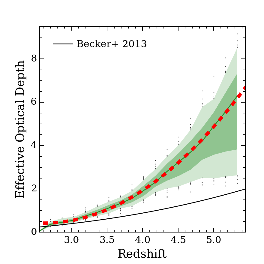
We create one simulated ‘skewer’ to match each GGG quasar sightline. The optical depth due to Ly, , is calculated along this skewer from just above the largest quasar redshift in the GGG sample, , down to , which corresponds to the blue cutoff of the GMOS spectra at 4620 Å. We measure the median effective optical depth as a function of redshift for the ensemble of skewers, where is the fraction of quasar flux transmitted, given by . We then compare this to the observed optical depth from Becker et al. (2013). The result is shown in Fig. 16. The effective optical depth for the mocks is about twice as large as the observed value at , and this discrepancy increases with redshift. Therefore, we apply a redshift-dependent scaling to the optical depth in the simulated skewers such that the median after scaling matches the Becker et al. relationship. We apply this scaling by fitting a second order polynomial to the ensemble median effective , and then multiplying by the Becker et al. (2013) relation and dividing by the polynomial fit.
Once we have corrected , we introduce absorption from the higher order Lyman series using wavelengths and oscillator strengths from Morton (2003). To identify Lyman limit systems and measure an approximate column density distribution, we identify peaks in the distribution and convert these to a column density using the relation from Draine (2011), assuming km s-1. This approximation will be relatively accurate for lines which have a much higher optical depth than the median value, but is likely to break down for low column density systems which are strongly blended (i.e. ). We then add Lyman continuum absorption for all systems with a Lyman limit optical depth 0.01. By visual inspection of the mock spectra, we found that the resulting transmission spectra contained too little absorption at wavelengths shorter than the quasar Lyman limit, which implies that there are too few strong absorbers and LLSs ( cm-2). These attenuate a significant amount of flux at such wavelengths. Because the simulations do not include radiative transfer calculations or use a self-shielding prescription, this lack of higher column density absorbers is unsurprising: high density clouds will be artificially highly ionised in the simulations.
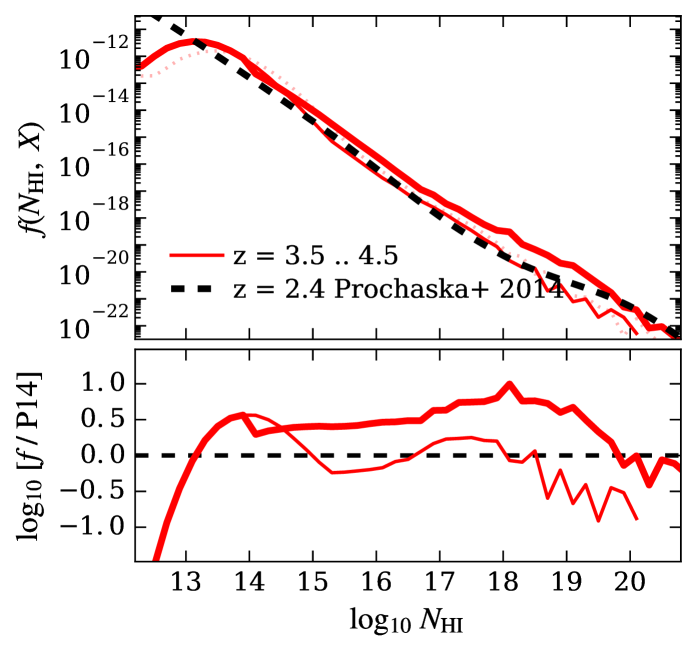
We test this idea with Fig. 17 where the thin solid (red) line shows the column density distribution per unit absorption distance in the simulations over the range compared to the observed distribution at from Prochaska et al. (2014). We assume that there is little evolution in the distribution shape between to apart from a change in the normalization corresponding to the evolution. In this case there does indeed appear to be a deficit of systems with cm-2 and cm-2. To correct this deficit, we multiply the column density of peaks by an amount which changes with column density, i.e. we add an offset of (0, 1, 2.2, 2) to for each system at reference values of (14, 15, 16, 18) and a linearly interpolated offset for systems with other values. These reference values were chosen arbitrarily, to provide enough flexibility to adjust the column densities in the range to better match the observed column density distribution. The offsets at these reference values were found by generating many sets of mock spectra in a parameter grid of offset values, and choosing the set of offset parameters such that a rest-frame average of the mock spectra matched a rest frame average of the real spectra in the Lyman limit region (–Å, see Fig. 18). Applying this correction produces the column density distribution shown by the thick solid (red) line in Fig. 17. This correction flattens out the ‘dips’ in the high ranges such that it better matches the shape of the observed distribution.
A.2 Simulations used for the mock spectra
The simulations were run using the open-source, cosmological adaptive mesh refinement and N-body code, enzo444http://enzo-project.org, which is fully described in Bryan et al. (2014). To solve the hydrodynamics, we use the Piecewise Parabolic Method of Woodward & Colella (1984). To compute the radiative heating and cooling of the gas, we use the grackle555https://grackle.readthedocs.org chemistry and cooling library (version 2.1, Bryan et al., 2014; hoon Kim et al., 2013; Smith et al., 2017). We use the primordial chemistry solver in the grackle library to calculate the non-equilibrium evolution of H i, H ii, He i, He ii, He iii, and electrons. The heating and cooling from metals is included by interpolating from multi-dimensional tables created with the photo-ionization code, cloudy (Ferland et al., 2013). For both the primordial elements and metals, we include photo-ionisation and photo-heating from the UV background model of Haardt & Madau (2012). We include the effects of star formation and feedback following the model of Dalla Vecchia & Schaye (2012), whereby thermal energy is injected in the grid cell hosting a star particle to a level high enough to make the sound crossing time shorter than the cooling time, a numerically-based criterion that Dalla Vecchia & Schaye (2012) have shown to be successful at creating realistic outflows.
The simulation consists of a 100 Mpc/h box with 2563 dark matter particles and grid cells on the root grid. We zoom into a region 25 Mpc/h on a side with two nested refinement levels, each refining by a factor of 2 in length, or 8 in mass. The dark matter particle mass within the high-resolution region is roughly 3 M⊙. We allow 5 additional levels of adaptive mesh refinement for a maximum spatial resolution of 2 kpc/h. The high-resolution region was chosen such that it represents an average region within the larger 100 Mpc/h box. The simulation and all associated methods will be described in full detail in Smith & Khochfar (in preparation).
The spectra are generated using the yt666http://yt-project.org simulation analysis toolkit (Turk et al., 2011). Each spectrum consists of a line of sight created in the method described by Smith et al. (2011) and updated by Hummels et al. (2017), in which multiple outputs from the simulation are used to span the redshift range from z = 5.5 to 3. At each redshift interval, each line of sight is randomly oriented to minimize sampling the same structures and only the high resolution region is used. For each grid cell intersected by the line of sight, we extract the H i number density, temperature, velocity, and redshift, and insert an appropriately shifted Voigt profile in a synthetic spectrum.
A.3 Comparison between the mock and observed LLS distribution
Our aim is for the LLS distribution in the mock spectra to match the distribution of the real LLSs as closely as possible. If this is the case, we can be more confident that the correction factors we derive from the observed to the true in the mocks will also be applicable to the real GMOS spectra.
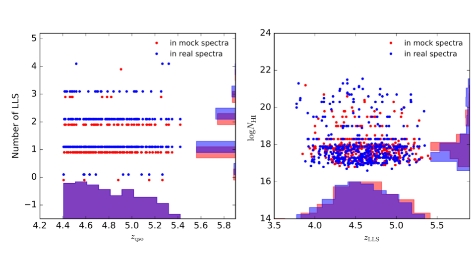
In Fig. 19 we compare the redshift distribution, the number of LLSs per sightline, and the column density distribution of the identified LLSs for in the mock sample and real spectra. The redshift distribution for LLSs in the real and mock spectra are very similar. The number of LLSs per sightline are also similar, although there tend to be slightly fewer mock sightlines with 2 or more LLSs compared to the real sightlines. The distribution is similar, although somewhat more partial LLSs () are identified in the mock spectra compared to those found in the real spectra. Through these checks, together with a visual comparison of each real and mock spectrum, we conclude that the LLS distribution in the mock spectra match the distribution observed in the real spectra closely enough to derive a reliable correction factor for .
References
- Abazajian et al. (2009) Abazajian K. N., et al., 2009, ApJS, 182, 543
- Astropy Collaboration et al. (2013) Astropy Collaboration et al., 2013, A&A, 558, A33
- Bahcall & Peebles (1969) Bahcall J. N., Peebles P. J. E., 1969, ApJ, 156, L7
- Bechtold et al. (1984) Bechtold J., Green R. F., Weymann R. J., Schmidt M., Estabrook F. B., Sherman R. D., Wahlquist H. D., Heckman T. M., 1984, ApJ, 281, 76
- Becker et al. (2013) Becker G. D., Hewett P. C., Worseck G., Prochaska J. X., 2013, Monthly Notices of the Royal Astronomical Society, 430, 2067
- Behrens et al. (2018) Behrens C., Byrohl C., Saito S., Niemeyer J. C., 2018, A&A, 614, A31
- Bryan et al. (2014) Bryan G. L., et al., 2014, ApJS, 211, 19
- Crighton et al. (2015) Crighton N. H. M., et al., 2015, Mon. Not. R. Astron. Soc., 452, 217
- Crighton et al. (2016) Crighton N. H. M., O’Meara J. M., Murphy M. T., 2016, MNRAS, 457, L44
- Dalla Vecchia & Schaye (2012) Dalla Vecchia C., Schaye J., 2012, MNRAS, 426, 140
- Draine (2011) Draine B. T., 2011, Physics of the Interstellar and Intergalactic Medium
- Faucher-Giguère & Kereš (2011) Faucher-Giguère C.-A., Kereš D., 2011, MNRAS, 412, L118
- Faucher-Giguere et al. (2007) Faucher-Giguere C. ., Lidz A., Zaldarriaga M., Hernquist L., 2007, ArXiv Astrophysics e-prints,
- Ferland et al. (2013) Ferland G. J., et al., 2013, Rev. Mex. Astron. Astrofis., 49, 137
- Fumagalli et al. (2011a) Fumagalli M., O’Meara J. M., Prochaska J. X., 2011a, Science, 334, 1245
- Fumagalli et al. (2011b) Fumagalli M., Prochaska J. X., Kasen D., Dekel A., Ceverino D., Primack J. R., 2011b, MNRAS, 418, 1796
- Fumagalli et al. (2013) Fumagalli M., O'Meara J. M., Prochaska J. X., Worseck G., 2013, ApJ, 775, 78
- Fumagalli et al. (2016) Fumagalli M., O’Meara J. M., Prochaska J. X., 2016, MNRAS, 455, 4100
- Garnett et al. (2017) Garnett R., Ho S., Bird S., Schneider J., 2017, MNRAS, 472, 1850
- Haardt & Madau (2012) Haardt F., Madau P., 2012, ApJ, 746, 125
- Hennawi & Prochaska (2007) Hennawi J. F., Prochaska J. X., 2007, ApJ, 655, 735
- Hummels et al. (2017) Hummels C. B., Smith B. D., Silvia D. W., 2017, ApJ, 847, 59
- Hunter (2007) Hunter J. D., 2007, Computing in Science and Engineering, 9, 90
- Inoue et al. (2014) Inoue A. K., Shimizu I., Iwata I., Tanaka M., 2014, MNRAS, 442, 1805
- Lanzetta (1991) Lanzetta K. M., 1991, ApJ, 375, 1
- Lehner et al. (2014) Lehner N., O’Meara J. M., Fox A. J., Howk J. C., Prochaska J. X., Burns V., Armstrong A. A., 2014, ApJ, 788, 119
- McQuinn et al. (2011) McQuinn M., Oh S. P., Faucher-Giguère C.-A., 2011, ApJ, 743, 82
- Morton (2003) Morton D. C., 2003, The Astrophysical Journal Supplement Series, 149, 205
- O’Meara et al. (2013) O’Meara J. M., Prochaska J. X., Worseck G., Chen H.-W., Madau P., 2013, ApJ, 765, 137
- Parks et al. (2018) Parks D., Prochaska J. X., Dong S., Cai Z., 2018, MNRAS, 476, 1151
- Peroux et al. (2003) Peroux C., Dessauges-Zavadsky M., D'Odorico S., Kim T.-S., McMahon R. G., 2003, Monthly Notices RAS, 345, 480
- Péroux et al. (2006) Péroux C., Kulkarni V. P., Meiring J., Ferlet R., Khare P., Lauroesch J. T., Vladilo G., York D. G., 2006, A&A, 450, 53
- Prochaska (1999) Prochaska J. X., 1999, ApJ, 511, L71
- Prochaska et al. (2006) Prochaska J. X., O’Meara J. M., Herbert-Fort S., Burles S., Prochter G. E., Bernstein R. A., 2006, ApJ, 648, L97
- Prochaska et al. (2010) Prochaska J. X., O'Meara J. M., Worseck G., 2010, ApJ, 718, 392
- Prochaska et al. (2013) Prochaska J. X., et al., 2013, ApJ, 776, 136
- Prochaska et al. (2014) Prochaska J. X., Madau P., O’Meara J. M., Fumagalli M., 2014, MNRAS, 438, 476
- Prochaska et al. (2015) Prochaska J. X., O’Meara J. M., Fumagalli M., Bernstein R. A., Burles S. M., 2015, ApJS, 221, 2
- Rahmati et al. (2013) Rahmati A., Pawlik A. H., Raičević M., Schaye J., 2013, MNRAS, 430, 2427
- Rahmati et al. (2015) Rahmati A., Schaye J., Bower R. G., Crain R. A., Furlong M., Schaller M., Theuns T., 2015, MNRAS, 452, 2034
- Ribaudo et al. (2011) Ribaudo J., Lehner N., Howk J. C., 2011, ApJ, 736, 42
- Rogers et al. (2018a) Rogers K. K., Bird S., Peiris H. V., Pontzen A., Font-Ribera A., Leistedt B., 2018a, MNRAS, 474, 3032
- Rogers et al. (2018b) Rogers K. K., Bird S., Peiris H. V., Pontzen A., Font-Ribera A., Leistedt B., 2018b, MNRAS, 476, 3716
- Sargent et al. (1989) Sargent W. L. W., Steidel C. C., Boksenberg A., 1989, ApJS, 69, 703
- Shukla et al. (2016) Shukla H., Mellema G., Iliev I. T., Shapiro P. R., 2016, Mon. Not. R. Astron. Soc., p. stw249
- Smith et al. (2011) Smith B. D., Hallman E. J., Shull J. M., O’Shea B. W., 2011, ApJ, 731, 6
- Smith et al. (2017) Smith B. D., et al., 2017, MNRAS, 466, 2217
- Songaila & Cowie (2010) Songaila A., Cowie L. L., 2010, ApJ, 721, 1448
- Steidel (1990) Steidel C. C., 1990, ApJS, 74, 37
- Stengler-Larrea et al. (1995) Stengler-Larrea E. A., et al., 1995, ApJ, 444, 64
- Turk et al. (2011) Turk M. J., Smith B. D., Oishi J. S., Skory S., Skillman S. W., Abel T., Norman M. L., 2011, ApJS, 192, 9
- Tytler (1982) Tytler D., 1982, Nature, 298, 427
- Woodward & Colella (1984) Woodward P., Colella P., 1984, Journal of Computational Physics, 54, 115
- Worseck & Prochaska (2011) Worseck G., Prochaska J. X., 2011, ApJ, 728, 23
- Worseck et al. (2014) Worseck G., et al., 2014, Monthly Notices of the Royal Astronomical Society, 445, 1745
- Zheng & Miralda-Escudé (2002) Zheng Z., Miralda-Escudé J., 2002, ApJ, 568, L71
- hoon Kim et al. (2013) hoon Kim J., et al., 2013, ApJS, 210, 14